Parallel Algorithms for Geometric Graph Problems

Abstract

We give algorithms for geometric graph problems in the modern parallel models such as MapReduce [DG04, KSV10, GSZ11, BKS13]. For example, for the Minimum Spanning Tree (MST) problem over a set of points in the two-dimensional space, our algorithm computes a $(1+\epsilon)$-approximate MST. Our algorithms work in a constant number of rounds of communication, while using total space and communication proportional to the size of the data (linear space and near linear time algorithms). In contrast, for general graphs, achieving the same result for MST (or even connectivity) remains a challenging open problem [BKS13], despite drawing significant attention in recent years.

We develop a general algorithmic framework that, besides MST, also applies to Earth-Mover Distance (EMD) and the transportation cost problem. Our algorithmic framework has implications beyond the MapReduce model. For example it yields a new algorithm for computing EMD cost in the plane in near-linear time, $n^{1+o_{\epsilon}(1)}$. We note that while recently [SA12b] have developed a near-linear time algorithm for $(1+\epsilon)$-approximating EMD, our algorithm is fundamentally different, and, for example, also solves the transportation (cost) problem, raised as an open question in [SA12b]. Furthermore, our algorithm immediately gives a $(1+\epsilon)$-approximation algorithm with $n^{\delta}$ space in the streaming-with-sorting model with $1/\delta^{O(1)}$ passes. As such, it is tempting to conjecture that the parallel models may also constitute a concrete playground in the quest for efficient algorithms for EMD (and other similar problems) in the vanilla streaming model, a well-known open problem [McG06, IMNO11].

1 Introduction

Over the past decade a number of parallel systems have become widely successful in practice. Examples of such systems include MapReduce [DG04, DG08], Hadoop [Whi12], and Dryad [IBY⁺07]. Given these developments, it is natural to revisit algorithmics for parallel systems and ask what new algorithmic or complexity ideas Theoretical Computer Science can contribute to this line of research (and engineering) efforts.

Two theoretical questions emerge: 1) What models capture well the capabilities of the existing systems? 2) What new algorithmic ideas can we develop for these models? Addressing Question 1, researchers [FMS⁺10, KSV10, GSZ11, BKS13] have proposed a model which balances simplicity and relevance to practice. We describe this model later in Section 1.1. As for Question 2, while there already exist a few algorithms adapted or designed for this model (see Section 1.3), we feel that many more powerful algorithmic ideas are still waiting to be developed.

The first natural question to ask is: do we really need new algorithmics here? After all, we have had a lot of fundamental research done on parallel algorithms in 1980s and 1990s, most notably in the PRAM model, which one may hope to leverage to new models. Indeed, the works of [KSV10, GSZ11] have shown that one can simulate PRAM algorithms in MapReduce with minimal slow-down. So what is new?

The answer is that the parameters of the new models are such that we can hope for faster algorithms than those possible in the PRAM model. The models allow for interleaving parallel and sequential computation: in a single step, a machine can perform arbitrary polynomial time computation on its local input; the time cost of the algorithm is then measured in the number of rounds of communication between machines. This makes it possible to achieve constant parallel time for interesting problems, while in the PRAM model functions that depend on the entire input generally require logarithmic or larger parallel time. For example, even computing the XOR of $n$ variables requires near-logarithmic parallel-time on the most powerful CRCW PRAMs [BH89]. In contrast, in the new models, which are similar to a $n^{\alpha}$-fan-in circuit, one can trivially solve XOR in $O(1/\alpha)$ parallel time. Indeed, the MapReduce models rather fall under the blanket of the generic Bulk Synchronous Parallel (BSP) model [Val90], though this model has a number of parameters, and as such has not been thoroughly explored. In particular, few solutions to even very fundamental problems are known in the BSP models (see, e.g., [Goo99] for a sorting algorithm). The new models instead focus on a specific range of parameters and tradeoffs, making analysis more tractable.

The previous work on MapReduce models identifies a captivating challenge problem: connectivity in a sparse graph. While this problem has a classic logarithmic time PRAM algorithm [SV82] we do not know whether we can solve it faster in the new models [KSV10]. For this particular problem, though, recent results show logarithmic lower bounds for restricted algorithms [BKS13], suggesting that the negative answer may be more plausible.

Synopsis of contributions.

In this work, we focus on basic graph problems in the geometric setting, and show we can achieve $1+\epsilon$ approximation in a constant number of rounds. In fact, we develop a common algorithmic framework applicable to graph questions such as Minimum Spanning Tree and Earth-Mover Distance. Thus, while it may be hard to speed up standard graph algorithms (without geometric context) in MapReduce-like models [BKS13], our results suggest that speedups can be obtained if we manage to represent the graph in a geometric fashion (e.g., in a similarity space).

Our framework turns out to be quite versatile, and, in fact has implications beyond parallel computing. For example it yields a new algorithm for computing EMD (cost) in the plane in near-linear time, $n^{1+o_{\epsilon}(1)}$. We note that while recently [SA12b] have developed a near-linear time algorithm for $(1+\epsilon)$-approximating EMD, our algorithm is different, and, for example, also solves the transportation (cost) problem, raised as an open question in [SA12b]. In particular, our algorithm uses little of the combinatorial structure of EMD, and essentially relies only on an off-the-shelf LP solver. In contrast, [SA12b] intrinsically exploit the combinatorial structure, together with carefully designed data structures to obtain a $O_{\epsilon}(n\log^{O(1)}n)$ time algorithm. Their approach, however, seems hard to parallelize.

Another consequence is also a $1+\epsilon$ approximation algorithm in the streaming-with-sorting model, with $n^{\delta}$ space and $1/\delta^{O(1)}$ passes. Hence, our EMD result suggests the new parallel models as a concrete playground in the quest for an efficient streaming algorithm for EMD, a well-known open question [McG06, IMNO11].

1.1 The Model

We adopt the most restrictive MapReduce-like model among [KSV10, GSZ11, BKS13] (and BSP [Val90] for a specific setting of parameters). Following [BKS13], we call the model Massively Parallel Communication or MPC (although we explicitly consider the local sequential running times as well).

Suppose we have $m$ machines (processors) each with space $s$, where $n$ is the size of the input and $m\cdot s=O(n)$. Thus, the total space in the system is only a constant factor more than the input size, allowing for minimal replication.

The computation proceeds in rounds. In each round, a machine performs local computation on its data (of size $s$), and then sends messages to other machines for the next round. Crucially, the total amount of communication sent or received by a machine is bounded by $s$, its space. For example, a machine can send one message of size $s$, or $s$ messages of size $1$. It cannot, however, broadcast a size $s$ message to every machine. In the next round, each machine treats the received messages as the input for the round.

The main complexity measure is the number of rounds $R$ required to solve a problem, which we consider to be the “parallel time” of the algorithm. Some related models, such as BSP, also consider the sequential running time of a machine in a round. We will de-emphasize this aspect, as we consider the information-theoretic question of understanding the round complexity to be the first-order business here. In particular, the restriction on space alone (i.e., with unbounded computation per machine) already appears to make certain problems take super-constant number of rounds, including the connectivity in sparse graphs. Nevertheless it is natural to minimize the local running time, and indeed our (local) algorithms run in time polynomial in $s$, leading to $O(ns^{O(1)})$ overall work.

What are good values of $s$ and $R$? As in [KSV10, GSZ11], we assume that space $s$ is polynomial in $n$, i.e., $s=n^{\alpha}$ for some $\alpha>0$. We consider this a justified choice since even under the natural assumption that $s\geq m$ (i.e., each machine has an index of all other machines), we immediately obtain that $s\geq\sqrt{n}$.

Our goal is to obtain $R=\mathop{\rm{poly}}\nolimits(\log_{s}n)=O(1)$ rounds. Note that we do not hope to do better than $O(\log_{s}n)$ rounds as this is required even for computing the XOR of $n$ bits.

Finally, note that the total communication is, a fortiori, $O(n)$ per round and $O(nR)=O(n)$ overall.

Streaming models. The above MPC model essentially resides in between two streaming models.

First, it is at least as strong as the “linear streaming” model, where one stores a (small) linear sketch of the input: if one has a linear sketch algorithm using space $s$ and $R$ passes, then we also have a parallel algorithm with local space $s^{2}$ (and $m=O(n/s^{2})$ machines) and $O(R\log_{s}m)$ rounds.

Second, the above model can be simulated in the model of streaming with a sorting primitive [ADRR04]. The latter model is similar to the standard multi-pass streaming model, but allows for both annotating the stream with keys as we go through it and sorting the entire stream according to these keys. In particular, sorting is considered in this model to be just another pass. Then if we have a parallel algorithm with $s$ space and $R$ rounds, we also obtain a streaming-with-sorting algorithm with $O(s)$ space and $O(R)$ passes.

1.2 Our Results

In this work, we focus on graph problems for geometric graphs. We assume to have $n$ points immersed in a low-dimensional space, such as $\mathbb{R}^{2}$ or a bounded doubling dimensional metric. Then we consider the complete graph on these points, where the weight of each edge is the distance between its endpoints.

We give parallel algorithms for the following problems:

• Minimum Spanning Tree (MST): compute the minimum spanning tree on the nodes. Note that MST is related to the hierarchical agglomerative clustering with single linkage, a classic (and practical) clustering algorithm [Zah71, KT06].

  We show how to compute a $1+\epsilon$ approximate MST over $\mathbb{R}^{d}$ in $O(\log_{s}n)$ rounds, as long as $(1/\epsilon)^{O(d)}<s$. Note that the number of rounds does not depend on $\epsilon$ or $d$. We extend the result to the case of a general point set with doubling dimension $d$. All our algorithms run in time $s^{O(1)}(1/\epsilon)^{O(d)}$ per machine per round.

  We note that our algorithm outputs the actual tree (not just the cost) of size $\approx n$, meaning in particular that the output is also stored in a distributed manner. The algorithms appear in Section 3 and 6.

• Earth-Mover Distance (EMD): given an equipartition of the points into red and blue points, compute the min-cost red-blue matching. A generalization is the transportation distance, in which red and blue points have positive weights of the same total sum, and the goal is to find a min-cost matching between red and blue masses. EMD and its variants are a common metric in image vision [RTG00, GD05].

  We show how to approximate the EMD and transportation cost up to a factor of $1+\epsilon$ over $\mathbb{R}^{2}$ in $(\log_{s}n)^{O(1)}$ rounds, as long as $(\log n)^{(\epsilon^{-1}\log_{s}n)^{O(1)}}<s$. The running time per machine per round is polynomial in $s$. Note that, setting $s=2^{\log^{1-c}n}$ for small enough $c>0$, we obtain a (standard) algorithm with overall running time of $n^{1+o(1)}$ for any fixed $\epsilon>0$. Our algorithm can also be seen as an algorithm in the streaming-with-sorting model, achieving $n^{\delta}$ space and $1/\delta^{O(1)}$ rounds by setting $s=n^{\delta}$. Our algorithm does not output the actual matching (as [SA12b] do). The algorithm appears in Section 4.

All our algorithms fit into a general framework, termed Solve-And-Sketch, that we propose for such problems. The framework is naturally “parallelizable”, and we believe is resilient to minor changes in the parallel model definition. We describe the general framework in Section 2, and place our algorithms within this framework. The actual implementation of the framework in the MPC model is described in Section 5.

It is natural to ask whether our algorithms are optimal. Unfortunately, we do not know whether both approximation and small dimension are required for efficient algorithms. However, we show that if we could solve exact MST (cost) in $l_{\infty}^{O(\log n)}$, we could also solve sparse connectivity (in general graphs), for which we have indications of being impossible [BKS13]. We also prove a query-complexity lower bound for MST in spaces with bounded doubling dimension in the black-box distance oracle model. In this setting, both approximation and dimension restriction seem necessary. These results appear in Section 7.

1.3 Motivation and Comparison to Previous Work

The model perspective. [KSV10] have initiated the study of dense graph problems in the MapReduce model they define, showing constant-round algorithms for connected-components, MST, and other problems. In the dense setting, the parameters are such that $m\gg s\gg n$, where $n$ is the number of vertices and $m$ is the number of edges. In this case, the solution (the size of which is $O(n)$) fits on a single machine.

In this regime, the main technique is filtering (see also [LMSV11]), where one iteratively sparsifies the input until the entire problem fits on one machine, at which moment the problem is solved by a regular sequential algorithm. For example, for connected-components, one can just throw out edges locally, preserving the global connectivity, until the graph has size at most $s$.

Somewhat departing from this is the work of [EIM11], who give algorithms for $k$-median and $k$-center, using $s=O(k^{2}n^{\delta})$. Instead of filtering, they employ (careful) sampling to reduce the size of the input until it fits in one machine and can be solved sequentially. Note that, while the entire “solution” is of size $n\gg s$, the solution is actually represented by $k\ll s$ centers. [KMVV13] further generalize both the filtering and sampling approaches for certain greedy problems, again where the solution , of size $k\ll s$, is computed on a single machine at the end.

Also highly relevant are the now-classic results on coresets [AHPV05, FL11], which are generic representation of (subset of) input with the additional property of being mergeable. These are often implementable in the MapReduce model (in fact, [EIM11] can be seen as such an implementation). However, coresets have been mostly used for geometric problems (not graph problems), which often have a small solution representation.

We contrast the “dense” regime with the “sparse” regime where $s$ is much smaller than the size of the solution. Most notably, for the problem of computing the connected components in a sparse graph, we have no better algorithm than those following from the standard PRAM literature, despite a lot of attention from researchers. In fact, [BKS13] suggest it may be hard to obtain a constant parallel-time for this problem.

Our algorithms rather fall in the “sparse” regime, as the solution (representation) is larger than the local space $s$. As such, it appears hard to apply filtering/sampling technique that drops part of the input from consideration. Indeed, our approach can be rather seen as a generalization of the notion of coreset.

We also mention there are other related works in MapReduce-like models, e.g., [CKT10, BPT11, BKV12], but which achieve at least a logarithmic parallel time.

The problems perspective. While we are not aware of a previous study of geometric graph problems in the MapReduce models, these problems have been studied extensively in other standard models, including 1) near-linear time algorithms, and 2) streaming algorithms.

Linear time (approximate) algorithms for MST are now classic results [Vai88, CK93]. For EMD, it is only very recently that researchers found a near-linear time approximation algorithm [SA12b] (following a line of work on the problem [Vai89, AES00, VA99, AV04, Ind07, SA12a]). Our framework naturally leads to near-linear time algorithms.

In the streaming model, a generic approach to approximate a large class of geometric graph problems has been introduced in [Ind04]. The work of [Ind04] has generally obtained logarithmic approximation for many problems and subsequently there has been a lot of research on improving these algorithms. Most relevantly, [FIS08] have shown how to $1+\epsilon$ approximate MST cost. We note that their algorithm outputs the cost only and does not lead to an algorithm for computing the actual tree as we accomplish here.

Getting $1+\epsilon$ approximate streaming algorithm for EMD is a well-known open question [McG06, IMNO11]. The best known streaming algorithm obtains a $O(1/\delta)$ approximation in $n^{\delta}$ space for any $\delta>0$ [ADIW09].

Our algorithmic framework immediately leads to an algorithm for computing $1+\epsilon$ approximation in $n^{\delta}$ space and $1/\delta^{O(1)}$ passes in the streaming-with-sorting model. In general, our EMD result implies one of the following: either 1) it illustrates the new parallel models as a concrete mid-point in the quest for an efficient streaming algorithm for EMD, or 2) it separates the new parallel models from the linear streaming model, showing them as practical models for sublinear space computation which are strictly more powerful than streaming. We do not know which of these cases is true, but either would be an interesting development in the area of sublinear algorithms.

1.4 Techniques

We now describe the main technical ideas behind our algorithms. Our MST algorithm is simple, but requires some careful analysis, while the EMD algorithm is technically the most involved.

MST. To illustrate the main ideas involved in the algorithm it suffices to consider the problem over the 2D grid $[0,n]^{2}$. The framework consists of three conceptual parts: partition, local solution, and sketch. The partition will be a standard quadtree decomposition, where we impose a hierarchical grid, randomly shifted in the space. In particular, each cell of the grid is recursively partitioned into $\sqrt{s}\times\sqrt{s}$ cells, until cell size is $\sqrt{s}\times\sqrt{s}$. The partition is naturally represented by a tree of arity $s$.

The other two parts are the crux of the algorithm. Consider first the following recursive naïve algorithm. Going bottom-up from the leaves at every cell in the quadtree we compute the minimum spanning tree among the input points (local solution), and then send a sketch of this tree to the upper-level cell. The problem is solved recursively in the upper-level cell by connecting partial trees obtained from the lower level.

However, such an algorithm does not yield a $(1+\epsilon)$-approximation. While constructing minimum spanning tree in a cell, the limited local view may force us to make an irrevocably bad decision. In particular, we may connect the nodes in the current cell, which in the optimum solution are connected by a path of nodes outside the cell. Consider an example on Figure 2. If the four points in the MST instance form the corners of a 2x1 rectangle then with constant probability (over the choice of the random partition), the edges of length 1 will be cut by a higher level of the partition than the edges of length 2. If an algorithm commits to constructing a minimum spanning tree for subproblems, then the two solid edges will be selected before the dashed edges are considered. At the next level the algorithm will select one of the dashed edges, and the total cost of the tree will be 5. However, substituting the green edge for the red edge results in a tree of cost 4.

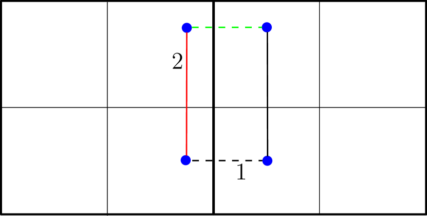
Figure 1: A bad example for the naïve MST algorithm.

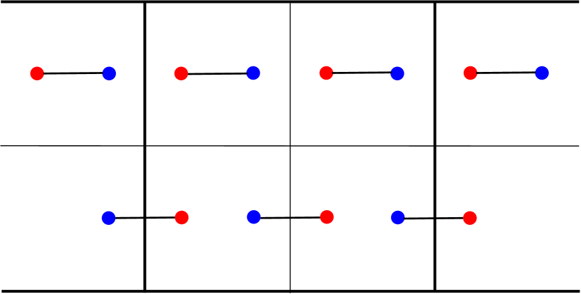
Figure 2: Local view is insufficient for EMD.

The challenge is to produce a local solution, without committing to decisions that may hurt in the future. To accomplish this, our local solution at a cell is to find the minimum spanning forest among the input points, using only short edges, of length at most $\epsilon$ times the diameter $\Delta$ of the cell. Note that it is possible that the local set of points remains disconnected.

Our sketch for each cell consists of an $\epsilon^{2}\Delta$-net of points in the cell together with the information about connectivity between them in the current partial solution. Note that the size of the sketch is bounded by $O(\epsilon^{-4})$. This sketch is sent to the parent cell. The local solution at the parent node now will consist of constructing a minimum spanning forest for the connected components obtained from its children.

In the analysis we argue that our algorithm is equivalent to Kruskal’s algorithm, but run on a graph with modified edge weights. We carefully construct the edge weights recursively to follow the execution of the algorithm. To prove the approximation guarantee, we make sure that the modified edge weights do not differ much from the original weights distances, in expectation, over the initial random shift.

We also generalize our algorithm to the case of a point set with bounded doubling dimension. Here, the new challenge is to construct a good hierarchical partition.

EMD. Our EMD algorithm adopts the general principle from MST, though the “solution” and “sketch” concepts become more intricate. Consider the case of EMD over $[n]^{2}$. As in MST, we partition the space using a hierarchical grid, represented by a tree with arity $s$.

In contrast to the MST algorithm, there are no local “safe” decisions one can make whatsoever. Consider Figure 2. The two rows of points are identical according to the local view. However, in one case we should match all points internally, and in the other, we should leave the end points to be matched outside. As far as the local view is concerned, either partial solution may be the right one. If we locally commit to the wrong one, we are not able to achieve a $1+\epsilon$ approximation no matter what we do next. This lack of “partial local solution” is perhaps the reason why EMD appears to be a much harder problem than even non-bipartite Euclidean matching, for which efficient algorithms have been known for a while now [Aro98].

It seems that we need to be able to sketch the entire set of local solutions. In particular, in the above case, we want to represent the fact that both (partial) matchings are valid (partial) solutions—as a function of what happens outside the local view—and include both of them in the sketch. Note that the two solutions from above have different “interfaces” with the outside world: namely the second one leaves two points to be matched to the outside.

And this is what we accomplish: we sketch the set of all possible local solutions. While reminiscent of the dynamic programming philosophy, our case is burdened by the requirement to represent this in sublinear (local) space. This seems like a daunting task: there are just too many potentially relevant local solutions. For example, consider a cell where we have $n/3$ red points close to the left border and $n/3$ blue points close to the right border. If there are some $k$ blue points to the left of the cell, and $k$ red ones to the right, then, inside the cell we should match exactly $n-k$ pairs of points. Hence, from a local viewpoint of the cell (which does not know $k$), there are $n/3$ potentially relevant local solutions. Sketching each one of them already takes space $\Omega(n)\gg s$.

Our algorithm manages to sketch this set of relevant local solutions approximately. Suppose we define a function $F$ of $d$ coordinates, one for “each position” in the local cell. In particular, $F$ takes as argument a vector $x\in\mathbb{Z}^{d}$ that specifies, for each $i\in[d]$, how many points are left unmatched at position $i$, with the convention that positive $x_{i}$ signifies red points and negative $x_{i}$ signifies blue points. Then we can define $F(x)$ to be the cost of the optimal matching of the rest of the points (with points specified by $x$ excluded from the local matching).

It would great to sketch the function $F:\mathbb{Z}^{d}\to\mathbb{R}_{+}$. Suppose we even reduced $d$ to be effectively $1/\epsilon^{2}$ (it suffices to consider only positions at the $\epsilon$-net of the cell, similarly to what happens in MST).

Nevertheless, even if $d=1/\epsilon^{2}$, we do not know how to sketch this function $F$. For example, even for a function $F$ of two parameters which is guaranteed to be monotone, convex, and Lipschitz, a concise sketch is generally not possible (in our case, $F$ is in fact not even monotone). What we show instead is that we can sketch the function $F^{\prime}(x)=F(x)+\|x\|_{1}\cdot A$, for some convenient factor $A$. It turns out that the additional term of $\|x\|_{1}\cdot A$ is tolerable as it will capture part of the cost of matching at the next level up. Then a sketch of $F^{\prime}$ can just consist of $F^{\prime}(x)$ values at $(\epsilon^{-1}\log n)^{O(d)}$ well-chosen $x$’s.

These ideas eventually lead to an information-theoretic algorithm for EMD, namely with the promised guarantees on space and rounds. It remains to make the running time of the local step polynomial in $s$. While computing $F^{\prime}(x)$ at a leaf is straight-forward (it’s essentially a matching), it is less clear for an internal node, where we have to compute $F^{\prime}(x)$ from the approximate sketches of $F^{\prime}_{j}$ of the node’s children $j\in J$.

To compute $F^{\prime}$ in polynomial time, we find the largest convex function which agrees with the sketch of each $F^{\prime}_{j}$; this gives a set of functions that are “piece-wise linear” and can be easily absorbed into a larger LP to compute $F^{\prime}$ at the internal node. We can do so because $F^{\prime}_{j}$ is a convex function, so the largest convex function that agrees with its sketch is sandwiched between the sketch itself and the actual $F^{\prime}_{j}$. In the end, the local running time is polynomial in $s$, because the resulting LPs can be solved with an arbitrary polynomial time LP algorithm.

We note that the total running time (work) is $n^{1+o(1)}$ (when setting $s=\log^{1-O(1)}n$), but we hope this can be brought down to $\tilde{O}(n)$ by exploiting more of the combinatorial structure of the problem and sketching $F$ or $F^{\prime}$ in space polynomial in $d$ (instead of exponential in $d$ as we do here).

1.5 Some Challenges For Future Research

We note that many research question remain open and may be relevant to both MapReduce/MPC-like models, as well as more generally to the area of sublinear algorithms. We list a few:

• Can we sketch the EMD partial solution(s) using $(\epsilon^{-1}\log n)^{O(1)}$ space? Can we compute the actual matching as well? This may lead to a $n(\epsilon^{-1}\log n)^{O(1)}$ overall time (work) for EMD and transportation problems (assuming the local running time is polynomial).

• More ambitiously, can these ideas lead to an efficient streaming algorithm for EMD, solving the open question of [McG06, IMNO11]? When do algorithms in our framework lead to streaming algorithms?

• Lower bounds: Is $1+\epsilon$ approximation or constant dimension required for geometric graph problem such as MST or EMD? What techniques need to be developed to prove such lower bounds?

• Can we solve data-structure like problems? In particular, some new systems allow for incremental updates to the input, with the expectation that the new computation be minimal (see, e.g., [MMI⁺13])?

2 Preliminaries: Solve-And-Sketch Framework

We now introduce the framework for our algorithms, termed Solve-And-Sketch. Its main purpose is to identify and decouple the crux of the algorithm for the specific problem from the implementation of the algorithm in the parallel model such as MPC.

The framework requires a “nice” hierarchical partition of the space. We view the hierarchical partition as a tree, where the arity is upper bounded by $\sqrt{s}$, and the depth is $O(\log_{s}n)$. The actual computation is broken down into small “local computational chunks”, arranged according to the hierarchical partitioning. The computation proceeds bottom-up, where at each node, the input (from below) is processed and the results are compressed into a small sketch that is sent up to the parent. Each level of the tree will be processed in parallel, with each node assigned to a machine.

In particular, the local computation at a node, termed “unit step”, consists of two steps:

1. Given the local inputs, we compute the set of partial or potential solutions. For leaves, the local information consists of the points in that part, and for internal nodes, it is the information obtained from the children.

2. Sketch the partial solution(s), using total space at most $p_{u}\leq\sqrt{s}$, and send this up the tree to the parent as a representation of solution(s) in this part.

The main challenges will be how to: 1) compute the partition, 2) define the right concept of “local solutions” in a part, and 3) sketch this concept as a sufficient representation of all potential solutions in this part. Often the naïve choice of the a local solution cannot be used, because it either ignores global information in a way that can damage the optimality of the algorithm, or it cannot be represented in sublinear space.

We now define more formally the notions of partition and of a unit step.

Hierarchical Partition. We use a hierarchical partition for inputs in $(\mathbb{R}^{d},\ell_{2})$ that is an analogue of a randomly-shifted quad-tree but a high branching factor (rather than the usual $2^{d}$). We denote the branching factor by $c$. We describe this partitioning scheme next (see Section 5.1 for additional details). The partitions we use to compute MST in a low doubling dimension metric space are more involved; see Section 6.

We assume that the points have integer coordinates in the range $[0,\Delta]$, where $\Delta=n^{O(1)}$. We show how to remove this bounded aspect ratio assumption in Section 5.2. Let $v\in\mathbb{R}^{d}$ be a vector chosen uniformly at random from $(-\Delta,0]^{d}$. We construct a hierarchical partition, denoted $P=(P_{0},\ldots,P_{L})$. The top level $P_{L}$ has a single part containing the whole input, and is identified with the cube $\{x:\forall i\ v_{i}\leq x_{i}\leq v_{i}+2\Delta\}$. Then we construct $P_{\ell-1}$ from $P_{\ell}$ by subdividing each cube associated with a part in $P_{\ell}$ into the $c$ equal sized cubes (via a grid with side-length $c^{1/d}$), thus creating a part associated with each smaller cube. In the final level $P_{0}$, each part is a singleton, i.e. all associated cubes contain at most a single point from the input. Since we assumed all points have integer coordinates in $[0,\Delta]$, it is enough to take $L=d\log_{c}\Delta=O(d\log_{c}n)$. For each level partition $P_{\ell}$, we call its parts as “cells”. For a cell $C\in P_{\ell}$, we can consider the subdivisions of the cell $C$ into next-level cells, i.e., all $C^{\prime}\in P_{\ell-1}$ such that $C^{\prime}\subseteq C$, which we call the “child cells” of $C$. For our implementation, we also need to label each child cell of $C$ with an integer in $[c]$. We can do this in a number of ways, for example, by lexicographic order on coordinates of the center of each cube associated with a child cell.

Unit Step. The other important component of the sketch and solve framework is the unit step, which is an algorithm $\mathcal{A}_{u}$ that is applied to each cell $C\in P_{\ell}$ for $\ell=1,\ldots,L$. At level $1$, $\mathcal{A}_{u}$ takes as input the points in $C$, and at level $\ell>1$, $\mathcal{A}_{u}$ takes as input the union of outputs of the unit steps applied to the children of $C$. The output of $\mathcal{A}_{u}$ on the top-most cell $P_{L}$ is the output of the problem (perhaps after some post-processing). We define functions $p_{u},t_{u},s_{u}$ as follows: on input of size $n_{u}$, $\mathcal{A}_{u}$ produces an output of size at most $p_{u}(n_{u})$, runs in time at most $t_{u}(n_{u})$, and uses a total space $s_{u}(n_{u})$. We require that, on empty input, $\mathcal{A}_{u}$ produces empty output. We call the algorithm that applies $\mathcal{A}_{u}$ to each cell of the partition in the above fashion the Solve-And-Sketch algorithm.

We prove that once we have a unit step algorithm for a problem, we also obtain a complete parallel algorithm for the said problem. Hence designing the unit step for a problem is the crux for obtaining a parallel algorithm and is decoupled from the actual implementation specifics in the considered parallel model.

Theorem 2.1 (Solve-And-Sketch).

Fix space parameter $s=(\log n)^{\Omega(d)}$ of the MPC model. Suppose there is a unit step algorithm using local time $t_{u}(n_{u})$, space $s_{u}(n_{u})$, and output size $p_{u}(n_{u})$ on input of size $n_{u}$. Assume the functions $t_{u},s_{u},p_{u}$ are non-decreasing, and also satisfy: $s_{u}(p_{u}(s))\leq s^{1/3}$ and $p_{u}(s)\leq s^{1/3}$. Then we can set $c=s^{\Theta(1)}$ and $L=O(\log_{s}n)$ in the partitioning from above, and we can implement the resulting Solve-And-Sketch algorithm in the MPC model in $(\log_{s}n)^{O(1)}$ rounds. Local runtime is $s\cdot t_{u}(s)\cdot(\log n)^{O(1)}$ (per machine per round).

The proof of the theorem is sensitive to the actual parallel model hence we defer it, along with other details of implementation in the MPC model, to Section 5. In the sections that follow, we describe how to implement the unit step algorithm for the two considered problems, which, by Theorem 2.1, will imply efficient MPC algorithm.

3 Minimum Spanning Tree

In this section we prove the existence of an efficient MPC algorithm that computes a spanning tree of a given point set in Euclidean space of approximately minimal cost.

Theorem 3.1.

Let $\epsilon>0$, and $s\geq(\epsilon^{-1}\log_{s}n)^{O(1)}$. Then there exists an MPC algorithm that, on input a set $S$ in $\mathbb{R}^{d}$ runs in $(\log_{s}n)^{O(1)}$ rounds and outputs a spanning tree of cost (under the Euclidean distance metric $\ell_{2}^{d}$ for $d=O(1)$) at most $1+\epsilon$ factor larger than the optimal. Moreover, the running time per machine is near linear in the input size $n_{u}$, namely $O(n_{u}\epsilon^{-d}\log^{O(1)}n_{u})$.

We prove the theorem above by exhibiting a unit step algorithm within the Solve-And-Sketch framework from Section 2. In fact our unit step algorithm will work with partitions more general than the quadtree-based partition described in Section 2. This will allows us to apply the unit step to point sets in low doubling dimension as well, once we have constructed an appropriate hierarchical partition. Details for the doubling dimension case appear in Section 6.

3.1 Hierarchical Partitions

Let us first define some metric geometry preliminaries and then define the general notion of partitions that our unit step algorithm uses.

We denote a metric space on a ground set $S$ with a distance function $\rho(\cdot,\cdot)$ as $M(S,\rho)$. For $S^{\prime}\subseteq S$ we denote the diameter of $S^{\prime}$ as $\Delta(S^{\prime})=\sup_{x,y\in S^{\prime}}\rho(x,y)$. A ball in $M$ centered in $x\in S$ with radius $r$ is denoted as $B_{M}(x,r)=\{y\in S|\rho(x,y)\leq r\}$. If the metric is clear from the context, we omit the subscript and write simply $B(x,r)$.

Definition 3.2 (Coverings, packings, and nets).

Let $M=(S,\rho)$ be a metric space and let $\delta$ and $\delta^{\prime}$ be positive reals. A set $S^{\prime}\subseteq S$ is a:

1. $\delta$-cover if for any point $x\in S$, there is a point $y\in S^{\prime}$ such that $\rho(x,y)\leq\delta$,

2. $\delta^{\prime}$-packing if for any two points $x,y\in S^{\prime}$, it holds that $\rho(x,y)\geq\delta^{\prime}$,

3. $(\delta,\delta^{\prime})$-net if it is both a $\delta$-covering and a $\delta^{\prime}$-packing,

4. $\delta$-net if it is a $(\delta,\delta)$-net.

Definition 3.3 (Doubling dimension).

The doubling dimension of a metric space is the smallest $d$ such that for all $r\geq 0$, any ball of radius $r$ can be covered with at most $2^{d}$ balls of radius $r/2$.

Lemma 3.4 (Dimension of restricted space).

Let $M_{1}=(S_{1},\rho)$ be a metric space of doubling dimension $d$. Let $M_{2}=(S_{2},\rho)$ be a metric space such that $S_{2}\subseteq S_{1}$. The doubling dimension of $M_{2}$ is at most $2d$.

Proof.

Consider an arbitrary ball $B_{M_{2}}(p,r)$ in $M_{2}$. Clearly, $B_{M_{2}}(p,r)\subseteq B_{M_{1}}(p,r)$. By definition, $B_{M_{1}}(p,r)$ can be covered with at most $(2^{d})^{2}$ balls $B_{1}$, …, $B_{k}$ of radius $r/4$ in $M_{1}$. Now, for each ball $B_{i}$ such that $B_{i}\cap S_{2}\neq\emptyset$, pick an arbitrary point $p_{i}\in B_{i}\cap S_{2}$.

We claim that the collection of balls $B_{M_{2}}(p_{i},r/2)$ for all such $i$ covers $B_{M_{2}}(p,r)$. Consider a point $p^{\prime}$ in $B_{M_{2}}(p,r)$. It belongs to a ball $B_{i}$. By the triangle inequality it holds $\rho(p^{\prime},p_{i})\leq r/2$, and therefore, $p^{\prime}$ belongs to $B_{M_{2}}(p_{i},r/2)$.

Summarizing, every ball $B_{M_{2}}(p,r)$ can be covered with at most $2^{2d}$ balls of radius $r/2$ in $M_{2}$, which implies that the doubling dimension of $M_{2}$ is at most $2d$.       

We use the following terminology to abstract out the common ideas behind our algorithms for Euclidean and bounded doubling dimension spaces. The common component of both algorithms is randomized hierarchical partition of the input space $M(S,\rho)$ (see, e.g. [Tal04]). A deterministic hierarchical partition $P$ with $L$ levels is defined as a sequence $P=(P_{0},\dots,P_{L})$, where $P_{L}=\{S\}$ and each level $P_{\ell}$ is a subdivision of $P_{\ell+1}$. For a partition $P_{i}$ we call its parts cells. The diameter at level $i$ is $\Delta(P_{i})=\max_{C\in P_{i}}\Delta(C)$. The degree of a cell $C\in P_{\ell}$ is $\operatorname{deg}(C)=|\{C^{\prime}\in P_{\ell-1}:C^{\prime}\subseteq C\}|$. The degree of a hierarchical partition is the maximum degree of any of its cells. We denote the unique cell at level $\ell$ containing a point $x$ as $C_{\ell}(x)$, i.e. $C_{\ell}(x)$ is defined by $x\in C_{\ell}(x)$ and $C_{\ell}(x)\in P_{\ell}$. For $\ell^{\prime}\leq\ell$ and $C\in P_{\ell^{\prime}}$ we define $C_{\ell}(C)$ analogously as the unique cell in the level $\ell$ containing $C$. We will also work with randomized hierarchical partitions which we treat as distributions over deterministic hierarchical partitions. We will denote such distributions as $\mathcal{P}$ to distinguish them from deterministic partitions.

Definition 3.5 (Distance-preserving hierarchical partition).

For $a,b\in(0,1)$, $\gamma>1$ a randomized hierarchical partition $\mathcal{P}$ of a metric space $M(S,\rho)$ with $L$ levels is $(a,b)$-distance-preserving with approximation $\gamma$ if every deterministic partition $P=(P_{0},\dots,P_{L})$ in its support satisfies the following properties for $\Delta_{\ell}=\gamma a^{L-\ell}\Delta(S)$:

1. (Bounded diameter) For all $\ell\in\{0,\dots,L\}$:

   $$\Delta(P_{\ell})\leq\Delta_{\ell}.$$

2. (Probability of cutting an edge) For every $x,y\in S$:

   $$\Pr[C_{\ell}(x)\neq C_{\ell}(y)]\leq b\frac{\rho(x,y)}{\Delta_{\ell}}.$$

To simplify the presentation we will refer to an $(a,b)$-distance preserving hierarchical partition as just $(a,b)$-partition. The parameter $\gamma$ plays a less important role in our proofs so we omit it to simplify presentation. Moreover, if an $(a,b)$-partition has degree $c$ we will call it just an $(a,b,c)$-partition. An example of a randomized $(a,b,c)$-partition is a randomly shifted and rotated quadtree in the Euclidean space $(\mathbb{R}^{d},\ell_{2})$, which is a $(1/2,O(d),2^{d})$-partition The Euclidean hierarchical partition described in Section 2 is an $(c^{-1/d},O(d),c)$-partition: see Section 5.1 for a detailed discussion.

3.2 The Unit Step Algorithm

Our Solve-and-Sketch (SAS) algorithm for computing an approximate minimum spanning tree (MST) works with a partition $P=(P_{0},\ldots,P_{L})$ of the input $M(S,\rho)$, sampled from a randomized $(a,b,c)$-partition $\mathcal{P}$. Recall that a SAS algorithm proceeds through $L$ levels, and in level $\ell$ a unit step algorithm is executed in each cell $C$ of the partition $P_{\ell}$, with input the union of the outputs of the unit steps applied to the children of $C$. Our MST unit step also outputs a subset of the edges of a spanning tree in addition to the input for the next level. In particular, the unit step computes a minimum spanning forest of the (possibly disconnected) subgraph consisting of edges between points in the cell of length at most an $\epsilon\Delta_{\ell}$. By not including longer edges we ensure that ignoring the edges that cross cell boundaries does not cost us a constant factor in the quality of the approximation (see Figure 2). The edges of the computed minimum spanning forest are output as a part of the constructed spanning tree. For the next level we output an $\epsilon^{2}\Delta_{\ell}$-covering of points in the cell, annotated by the connected components of the minimum spanning forest. In a space of constant dimension we can construct such covering of size $\epsilon^{-O(1)}$. The reason why the distance information given by the covering is accurate enough for our approximation is that all edges between different connected components in the spanning forest constructed so far are either long or have been crossing in the previous level.

We describe the unit step as Algorithm 1. Then Theorem 3.1 will follow from Theorem 2.1 and the guarantees on space and time complexity, as well as the approximation guarantees, for Algorithm 1.

1

input : Cell $C\in P_{\ell}$; a collection $V(C)$ of points in $C$, and a partition $Q=\{Q_{1},\ldots Q_{k}\}$ of $V(C)$ into previously computed connected components.

2

3repeat

4       Let $\tau=\min_{\begin{subarray}{c}i,j\\ i\neq j\end{subarray}}\min_{u\in Q_{i},v\in Q_{j}}\rho(u,v)$.

5       Find $u\in Q_{i}$ and $v\in Q_{j}$ for some $i,j:i\neq j$ such that $\rho(u,v)\leq(1+\epsilon)\tau$.

6       Let $\theta=\rho(u,v)$.

7       if $\theta\leq\epsilon\Delta_{\ell}$ then

8             Output tree edge $(u,v)$.

9             Merge $Q_{i}$ and $Q_{j}$ and update $Q$.

10            

11      

12until $\theta>\epsilon\Delta_{\ell}$

output : $V^{\prime}\subseteq V$, an $\epsilon^{2}\Delta_{\ell}$-covering for $C$, the partition $Q(V^{\prime})$ induced by $Q$ on $V^{\prime}$.

Algorithm 1 Unit Step at Level $\ell$

Notice that Algorithm 1 implements a variant of Kruskal’s algorithm, with the caveats that we ignore edges longer than $\epsilon\Delta_{\ell}$ as well as edges crossing the boundary of $C$, and that we also join only the approximately closest pair of connected components, rather than the closest pair. This last choice is made in order to allow us to use algorithms for approximate nearest neighbor search [Ind00, HPIM12] in order to identify which connected components to connect, and thus achieve near-linear total running time.

Let $T^{*}$ be some optimum minimum spanning tree. For a tree $T$, let $\rho(T)$ denote the cost of the tree $\rho(T)=\sum_{(u,v)\in T}\rho(u,v)$. The following theorem is our main approximation result for the SAS algorithm with unit step Algorithm 1.

Theorem 3.6.

Let $\mathcal{P}$ be a randomized $(a,b)$-partition of $M(S,\rho)$ with $L$ levels. If $a\leq\frac{1}{2}$ and $\epsilon\leq\frac{1}{4}$ then the spanning tree $T^{\circ}$ output by the Solve-and-Sketch algorithm with partition $P$ sampled from $\mathcal{P}$ and unit step Algorithm 1 satisfies:

$$\mathop{\mathbb{E}}\displaylimits_{P\sim\mathcal{P}}\left[\rho(T^{\circ})\right]\leq(1+\epsilon O(Lb))\rho(T^{*}).$$

It is natural to attempt to prove Theorem 3.6 by relating the SAS algorithm with unit step Algorithm 1 to a known MST algorithm, e.g. Kruskal’s algorithm (which our algorithm most closely resembles). There are several difficulties, arising from approximations that we use in order to achieve efficiency in terms of communication, running time, and space. For example, our algorithm only keeps progressively coarser coverings of the input between phases, and thus does not have exact information about distances between connected components. Nevertheless, it is known that an approximate implementation of Kruskal’s algorithm still outputs an approximate MST[Ind00, Section 3.3.1]. In particular, an algorithm that keeps a spanning forest, initially the empty graph, and at each time step connects any two connected components of the current forest that are at most a factor of $1+\epsilon$ further apart than the closest pair of connected components, computes a spanning tree of cost at most a factor $1+\epsilon$ larger than the cost of the MST. However, our setting presents a further difficulty: because we work in a parallel environment, Algorithm 1 completely ignores any edges crossing the boundary of the cell it is currently applied to. Such edges could have small length, which makes it generally impossible to show that our algorithm implements Kruskal’s algorithm even approximately for the complete graph with edge weights given by the metric $\rho$. Instead, we are able to relate our algorithm to a run of Kruskal’s algorithm on the complete graph with modified edge weights $w_{P}:S\times S\rightarrow\mathbb{R}_{+}$. These weights are a function of the hierarchical partition $P$; they are always an upper bound on the metric $\rho$, and give larger weight to edges that cross the boundaries of $P_{\ell}$ for larger $\ell$ (see Definition 3.9). We are able to show (Lemma 3.19) that the length (under $\rho$) of the $i$-th edge output by (a sequential simulation) of our algorithm is at most a factor $1+\epsilon$ larger than the weight (under $w_{P}$) of the $i$-the edge output by Kruskal’s algorithm, when run on the complete graph with edge weights $w_{P}$. The proof is then completed by arguing that for each $u,v\in S$, $w_{P}(u,v)$ approximates $\rho(u,v)$ in expectation when $P$ is sampled from a distance preserving partition (Lemma 3.10).

We define the following types of edges based on the position of their endpoints with respect to the space partition used by the algorithm.

Definition 3.7 (Crossing and non-crossing edges).

An edge $(u,v)$ is crossing in level $\ell$ if $C_{\ell}(u)\neq C_{\ell}(v)$ and non-crossing otherwise.

Also for each edge we define the crossing level, which will be useful in the analysis:

Definition 3.8 (Crossing level).

For an edge $(u,v)$ let its crossing level ${\ell_{c}}(u,v)$ be the largest integer such that $C_{{\ell_{c}}(u,v)}(u)\neq C_{{\ell_{c}}(u,v)}(v)$.

The modified weights $w$, which we use in the analysis, are defined for each pair $(u,v)$ using its crossing level as follows:

Definition 3.9 (Modified weights).

Let $\mathcal{P}$ be a randomized $(a,b)$-partition of $M(S,\rho)$ with $L$ levels. For every deterministic partition $P$ in the support of $\mathcal{P}$ we define $w_{P}(u,v)=\rho(u,v)+\epsilon\Delta_{{\ell_{c}}(u,v)}$.

We show that the modified weights $w_{P}(u,v)$ approximate the original distances $\rho(u,v)$ in expected value. This lemma and its proof are similar to arguments used in recent work on approximating the Earth-Mover Distance in near-linear time [SA12b], and dating back to Arora’s work on approximation algorithms for the Euclidean Traveling Salesman Problem [Aro98].

Lemma 3.10.

For all $u,v\in S$:

$$\rho(u,v)\leq\mathop{\mathbb{E}}\displaylimits_{P\sim\mathcal{P}}\left[w_{P}(u,v)\right]\leq(1+\epsilon Lb)\rho(u,v).$$

Proof.

The lower bound $\mathop{\mathbb{E}}\displaylimits_{P\sim\mathcal{P}}\left[w_{P}(u,v)\right]\geq\rho(u,v)$ follows from Definition 3.9 since $\Delta_{{\ell_{c}}(u,v)}\geq 0$. For the upper bound we use the properties of $(a,b)$-partitions. We have:

$$\mathop{\mathbb{E}}\displaylimits_{P\sim\mathcal{P}}\left[w_{P}(u,v)\right]=\mathop{\mathbb{E}}\displaylimits_{P\sim\mathcal{P}}\left[\rho(u,v)+\epsilon\Delta_{{\ell_{c}}(u,v)}\right]$$

$$=\rho(u,v)+\sum_{\ell=1}^{L}{\Pr_{P\sim\mathcal{P}}[{\ell_{c}}(u,v)=t]\epsilon\Delta_{\ell}}$$

$$=\rho(u,v)+\sum_{\ell=1}^{L}\Pr_{P\sim\mathcal{P}}\left[C_{\ell}(u)\neq C_{\ell}(v),C_{\ell+1}(u)=C_{\ell+1}(v)\right]\epsilon\Delta_{\ell}$$

$$\leq\rho(u,v)+\sum_{\ell=1}^{L}{\Pr_{P\sim\mathcal{P}}[C_{\ell}(u)\neq C_{\ell}(v)]\epsilon\Delta_{\ell}}$$

$$\leq\rho(u,v)+\sum_{\ell=1}^{L}{\epsilon b\rho(u,v)}$$

$$=\rho(u,v)(1+\epsilon Lb),$$

where the first equality follows from Definition 3.9, the second equality is an expansion of the expectation, the third equality follows from Definition 3.8, the fourth inequality follows from a term-by-term estimation of the probability of a joint event by the probability of one of its sub-events, the fifth inequality follows from the bound on the probability of cutting an edge for an $(a,b)$-partition (Definition 3.5) and the last one is a direct calculation.       

Recall that in Algorithm 1 for a cell $C\in P_{\ell}$ the set $V(C)$ is a subset of points of $C$ considered at level $\ell$. Also recall that $C_{\ell}(u)$ is the cell containing $u$ at level $\ell$. We use the following notation to denote the closest neighbor of $u$ considered at level $\ell$.

Definition 3.11 (Nearest neighbor at level $\ell$).

For $u\in S$ let $N_{\ell}(u)$ be the nearest neighbor to $u$ in $V(C_{\ell}(u))\cap C_{\ell-1}(u)$, i.e. $N_{\ell}(u)=\arg\min_{v\in V(C_{\ell}(u))\cap C_{\ell-1}(u)}\rho(u,v)$.

For two points $u,v$ we will use the following distance measure $\rho_{\ell}(u,v)$ in the analysis.

Definition 3.12 (Distance between nearest neighbors at level $\ell$).

For an edge $(u,v)$ we define $\rho_{\ell}(u,v)=\rho(N_{\ell}(u),N_{\ell}(v))$ to be the distance between the nearest neighbors of $u$ and $v$ at level $\ell$.

The next lemma shows that $\rho_{\ell}$ is an approximation to $\rho$.

Lemma 3.13.

For every $C\in P_{\ell}$ and $u,v\in C$ it holds that $|\rho_{\ell}(u,v)-\rho(u,v)|\leq 2\epsilon^{2}\Delta_{\ell-1}$.

Proof.

For each $C^{\prime}\in P_{\ell-1}$ such that $C^{\prime}\subseteq C$ by construction of the algorithm it holds that $V(C)\cap C^{\prime}$ is an $\epsilon^{2}\Delta_{\ell-1}$-covering for $C^{\prime}$. Thus, $V(C)$ is an $\epsilon^{2}\Delta_{\ell-1}$-covering for $C$. We have $\rho(N_{\ell}(u),u)\leq\epsilon^{2}\Delta_{\ell-1}$ and $\rho(N_{\ell}(v),v)\leq\epsilon^{2}\Delta_{\ell-1}$. By the triangle inequality we get $\rho(N_{\ell}(u),N_{\ell}(v))\leq\rho(N_{\ell}(u),u)+\rho(u,v)+\rho(N_{\ell}(v),v)\leq\rho(u,v)+2\epsilon^{2}\Delta_{\ell-1}$. By another application of triangle inequality we have $\rho(N_{\ell}(u),N_{\ell}(v))\geq\rho(u,v)-\rho(N_{\ell}(v),v)-\rho(N_{\ell}(u),u)\geq\rho(u,v)-2\epsilon^{2}\Delta_{\ell-1}$.       

To complete our analysis we need to further characterize edges according to their status during the execution of the algorithm.

Definition 3.14 (Short and long edges).

An edge $(u,v)$ is short in level $\ell$ if $\rho_{\ell}(u,v)\leq\frac{\epsilon}{1+\epsilon}\Delta_{\ell}$, and long otherwise.

Definition 3.15 (Processing level and sequence).

For an edge $e$ in $T^{\circ}$, the processing level $\ell_{p}(e)$ is the integer $\ell$, such that $e$ is output by the unit step applied to some $C\in P_{\ell}$. Consider a sequential simulation of the SAS algorithm with unit step Algorithm 1, in which at each level $\ell$, the unit step is applied to each cell $C\in P_{\ell}$ sequentially in an arbitrary order. The processing sequence $(e_{1},\ldots,e_{n-1})$ consists of the edges of $T^{\circ}$ in the order in which they are output by the above sequential simulation.

Definition 3.16 (Intercluster edges).

The forest at step $i$, denoted $T^{\circ}_{i}$, is defined as the forest $\{e_{1},\ldots,e_{i}\}$. An edge $e=(u,v)$ is intercluster at step $i$ if $u$ and $v$ lie in different connected components of $T^{\circ}_{i-1}$. We denote the set of all intercluster edges at step i as $I_{i}$.

Lemma 3.17.

Let $\epsilon\leq\frac{1}{4}$ and $a\leq\frac{1}{2}$. For every vertex $u$, level $\ell$ and step $i>1$ such that $\ell_{p}(e_{i})\geq\ell$ the vertices $u$ and $N_{\ell}(u)$ are in the same connected component of $T^{\circ}_{i-1}$.

Proof.

Note that it suffices to prove the claim for the smallest $i$ such that $\ell_{p}(e_{i})\geq\ell$. Fix such $i$. Assume for contradiction that for some $\ell$ the vertices $u$ and $N_{\ell}(u)$ are in different connected components of $T^{\circ}_{i-1}$. Fix the smallest such $\ell$. If $\ell=1$, then $N_{\ell}(u)=u$, so we may assume $\ell\geq 2$. Let $C=C_{\ell}(u)$ and $C^{\prime}=C_{\ell-1}(u)$. At the end of the execution of Algorithm 1 in cell $C^{\prime}$, the partition $Q$ of $V(C^{\prime})$ into connected components is a subdivision of the connected components of $T^{\circ}_{i-1}$ restricted to $V(C^{\prime})$. By the choice of $\ell$, $u$ and $N_{\ell-1}(u)$ are in the same connected component of $T^{\circ}_{i-1}$, and, since we assumed that $u$ and $N_{\ell}(u)$ are in different connected components of $T^{\circ}_{i-1}$, it must be the case that $N_{\ell-1}(u)$ and $N_{\ell}(u)$ are in different connected components in $Q$, i.e. $N_{\ell-1}(u)\in Q_{k}$ and $N_{\ell}(u)\in Q_{k^{\prime}}$ for $k\neq k^{\prime}$. Since $V(C)\cap C^{\prime}$ is a $\epsilon^{2}\Delta_{\ell-1}$-covering of $C^{\prime}$ and $V(C^{\prime})$ is a $\epsilon^{2}\Delta_{\ell-2}$-covering of $C^{\prime}$, we have $\rho(u,N_{\ell}(u))\leq\epsilon^{2}\Delta_{\ell-1}$ and $\rho(u,N_{\ell-1}(u))\leq\epsilon^{2}\Delta_{\ell-2}$. Then, by the triangle inequality, $\tau\leq\rho(N_{\ell-1}(u),N_{\ell}(u))\leq(1+a)\epsilon^{2}\Delta_{\ell-1}$, and the algorithm will find $u^{\prime}\in Q_{k},v^{\prime}\in Q_{k^{\prime}}$ such that $\theta=\rho(u^{\prime},v^{\prime})\leq(1+\epsilon)\tau\leq\epsilon^{2}(1+\epsilon)(1+a)\Delta_{\ell-1}$. Since for $\epsilon\leq\frac{1}{4}$ and $a\leq\frac{1}{2}$, $\epsilon(1+\epsilon)(1+a)<1$, this contradicts the termination condition for the main loop of Algorithm 1.       

Lemma 3.19 is the key part of the proof of Theorem 3.6. It shows that the cost of the $i$-th edge output by our algorithm is bounded in terms of the cost of $i$-th edge output by Kruskal’s algorithm.

Definition 3.18 (Kruskal’s edge at step $i$).

Let $e^{w_{P}}_{i}$ be the $i$-th edge output by Kruskal’s algorithm when run on the complete graph on $S$ with edge weights $w_{P}:S\times S\rightarrow\mathbb{R}$.

Lemma 3.19.

If $\epsilon\leq\frac{1}{4}$ and $a\leq\frac{1}{2}$, then for each $i$ it holds that $\rho(e_{i})\leq(1+O(\epsilon))w_{P}(e^{w_{P}}_{i}).$

Proof.

We denote the shortest intercluster edge at step $i$ as $e^{+}_{i}=\operatorname*{arg\,min}_{e\in I_{i}}w_{P}(e).$

First we show that the weight of $e^{w_{P}}_{i}$ is bounded by the weight of $e^{+}_{i}$ in Proposition 3.20. This argument is due to Indyk [Ind00, Section 3.3.1, Lemma 11].

Proposition 3.20.

For each $i$ it holds that $w_{P}(e^{+}_{i})\leq w_{P}(e^{w_{P}}_{i})$.

Proof.

Note that $T^{\circ}_{i-1}$ has $n-i+1$ connected components. Because $\{e^{w_{P}}_{1},\dots,e^{w_{P}}_{i}\}$ is a forest, there exists $j\leq i$ such the endpoints of $e^{w_{P}}_{j}$ lie in different connected components of $T^{\circ}_{i-1}$. Thus, by definition of $e^{+}$ we have $w_{P}(e^{+}_{i})\leq w_{P}(e^{w_{P}}_{j})$. Because the edges output by Kruskal’s algorithm satisfy that $w_{P}(e^{w_{P}}_{j})\leq w_{P}(e^{w_{P}}_{i})$ for $j\leq i$ the lemma follows.       

Using Proposition 3.20 it suffices to show that $\rho(e_{i})\leq(1+O(\epsilon))w_{P}(e^{+}_{i})$ to complete the proof. We consider three cases:

Case I: $\ell_{c}(e^{+}_{i})\geq\ell_{p}(e_{i})$.

In this case we have:

$$\rho(e_{i})\leq\epsilon\Delta_{\ell_{p}(e_{i})}\leq\rho(e^{+}_{i})+\epsilon\Delta_{\ell_{p}(e_{i})}\leq\rho(e^{+}_{i})+\epsilon\Delta_{{\ell_{c}}(e^{+}_{i})}=w_{P}(e^{+}_{i}),$$

where the first inequality follows from the condition for outputting the edges in Algorithm 1, the second one is since $\rho(e^{+}_{i})\geq 0$, the third one is because $\ell_{p}(e_{i})\leq{\ell_{c}}(e^{+}_{i})$ by assumption and the last one is by Definition 3.9. This completes the analysis of the first case.

The following proposition will be crucial for the analysis of the remaining two cases. It shows that the $i$-th edge $e_{i}$ output by (the sequential simulation) of the SAS algorithm is approximately the shortest non-crossing intercluster edge.

Proposition 3.21.

Let $\epsilon\leq\frac{1}{4}$ and $a\leq\frac{1}{2}$. If $e\in I_{i}$ is non-crossing at level $\ell_{p}(e_{i})$ then $\rho(e_{i})\leq(1+\epsilon)\rho_{\ell_{p}(e_{i})}(e)$.

Proof.

Fix $e=(u,v)$ and consider an edge $(u^{\prime},v^{\prime})$ where $u^{\prime}=N_{\ell_{p}(e_{i})}(u)$ and $v^{\prime}=N_{\ell_{p}(e_{i})}(v)$. By Lemma 3.17 we have that $u$ and $u^{\prime}$ are in the same connected component of $T^{\circ}_{i-1}$. Similarly $v$ and $v^{\prime}$ are also in the same connected component. By assumption $(u,v)\in I_{i}$ so these two connected components are different. Because the edge $(u,v)$ is non-crossing at level $\ell_{p}(e_{i})$ the edge $(u^{\prime},v^{\prime})$ is also non-crossing at this level. Thus,

$$\rho(e_{i})\leq(1+\epsilon)\tau\leq(1+\epsilon)\rho(N_{\ell_{p}(e_{i})}(u),N_{\ell_{p}(e_{i})}(v))=(1+\epsilon)\rho_{\ell_{p}(e_{i})}(e),$$

where the first inequality is by construction used in Algorithm 1, the second is by definition of $\tau$ together with the fact that $(u^{\prime},v^{\prime})$ is a non-crossing edge at level $\ell_{p}(e_{i})$ between two different connected components and the last is by Definition 3.12.       

Case II: $\ell_{c}(e^{+}_{i})=\ell_{p}(e_{i})-1$.

In this case we have:

$$\rho_{\ell_{p}(e_{i})}(e^{+}_{i}) \leq\rho(e^{+}_{i})+2\epsilon^{2}\Delta_{\ell_{p}(e_{i})-1}$$

$$<\rho(e^{+}_{i})+\epsilon\Delta_{\ell_{p}(e_{i})-1}+\epsilon^{2}\Delta_{\ell_{p}(e_{i})-1}$$

$$\leq(1+\epsilon)(\rho(e^{+}_{i})+\epsilon\Delta_{\ell_{p}(e_{i})-1})$$

$$=(1+\epsilon)w_{P}(e^{+}_{i}),$$

where the first line follows by Lemma 3.13, the second uses the assumption that $\epsilon<1$, the third follows since $\rho(e^{+}_{i})\geq 0$ and the last one holds by Definition 3.9 together with the assumption that $\ell_{c}(e^{+}_{i})=\ell_{p}(e_{i})-1$. By assumption $e^{+}_{i}$ is non-crossing at level $\ell_{p}(e_{i})$, and therefore Proposition 3.21 and the assumption $\epsilon\leq\frac{1}{2}$ imply

$$\rho(e_{i})\leq(1+\epsilon)\rho_{\ell_{p}(e_{i})}(e^{+}_{i})\leq(1+\epsilon)^{2}w_{P}(e^{+}_{i})\leq(1+\frac{5}{2}\epsilon)w_{P}(e^{+}_{i}).$$

Case III: $\ell_{c}(e^{+}_{i})<\ell_{p}(e_{i})-1$.

First, we prove the following auxiliary statement.

Proposition 3.22.

Let $\epsilon\leq\frac{1}{4}$ and $a\leq\frac{1}{2}$. Every $e\in I_{i}$ is either crossing or long in level $\ell_{p}(e_{i})-1$.

Proof.

Let the edge $e=(u,v)$ be short and non-crossing in level $\ell_{p}(e_{i})-1$. We will show that this implies that $u$ and $v$ are in the same connected component of $T^{\circ}_{i-1}$ and hence $e\notin I_{i}$. By Lemma 3.17, $u$ and $N_{\ell_{p}(e_{i})-1}(u)$ are in the same connected component of $T^{\circ}_{i-1}$. The same is true for $v$ and $N_{\ell_{p}(e_{i})-1}(v)$. Thus, it suffices to show that $N_{\ell_{p}(e_{i})-1}(u)$ and $N_{\ell_{p}(e_{i})-1}(v)$ are in the same connected component of $T^{\circ}_{i-1}$.

First, note that because the edge $(u,v)$ is non-crossing at level $\ell_{p}(e_{i})-1$, the edge $(N_{\ell_{p}(e_{i})-1}(u),N_{\ell_{p}(e_{i})-1})$ is also non-crossing at this level. Suppose for the sake of contradiction that $N_{\ell_{p}(e_{i})-1}(u)$ and $N_{\ell_{p}(e_{i})-1}(v)$ were in different connected components when Algorithm 1 finishes processing cells at level $\ell_{p}(e_{i})-1$. Then Algorithm 1 would have found vertices $u^{\prime}$ and $v^{\prime}$ in these components such that:

$$\rho(u^{\prime},v^{\prime})\leq(1+\epsilon)\tau\leq(1+\epsilon)\rho(N_{\ell_{p}(e_{i})-1}(u),N_{\ell_{p}(e_{i})-1}(v))=(1+\epsilon)\rho_{\ell_{p}(e_{i})-1}(u,v)\leq\epsilon\Delta_{\ell_{p}(e_{i})-1},$$

where the first inequality is by construction used in Algorithm 1, the second is by definition of $\tau$ together with the fact that $(N_{\ell_{p}(e_{i})-1}(u),N_{\ell_{p}(e_{i}-1})$ is non-crossing, the third equality is by Definition 3.12 and the fourth inequality is by assumption that $(u,v)$ is short and Definition 3.14. This contradicts the termination condition for Algorithm 1.

 

In this case, by Proposition 3.22, since $e^{+}_{i}$ was not crossing in level $\ell_{p}(e_{i})-1$, then $e^{+}_{i}$ must have been long. Thus,

$$\rho(e^{+}_{i}) \geq\rho_{\ell_{p}(e_{i}-1)}(e^{+}_{i})-\epsilon^{2}\Delta_{\ell_{p}(e_{i})-2}$$

$$>\frac{\epsilon}{1+\epsilon}\Delta_{\ell_{p}(e_{i})-1}-\epsilon^{2}\Delta_{\ell_{p}(e_{i})-2}$$

$$=\left(\frac{1}{1+\epsilon}-a\epsilon\right)\epsilon\Delta_{\ell_{p}(e_{i})-1}$$

$$>(1-(1+a)\epsilon)\epsilon\Delta_{\ell_{p}(e_{i})-1},$$

where the first inequality is by Lemma 3.13, the second inequality is by definition of a long edge at level $\ell_{p}(e_{i})-1$ (Definition 3.14) and the third equality is because for an $(a,b)$-partition it holds that $\Delta_{\ell_{p}(e_{i})-2}=a\Delta_{\ell_{p}(e_{i})-1}$.

Then we have:

$$\rho(e_{i}) \leq(1+\epsilon)\rho_{\ell_{p}(e_{i})}(e^{+}_{i})$$

$$\leq(1+\epsilon)\rho(e^{+}_{i})+(1+\epsilon)\epsilon^{2}\Delta_{\ell_{p}(e_{i})-1}$$

$$\leq\left(1+\left(1+\frac{1+\epsilon}{1-(1+a)\epsilon}\right)\epsilon\right)\rho(e^{+}_{i})$$

$$\leq(1+O(\epsilon))w_{P}(e^{+}_{i}),$$

where the first inequality is by Proposition 3.21, the second is by 3.13, the third is using the calculation above and the last one is a direct calculation.       

Proof of Theorem 3.6.

We have:

$$\mathop{\mathbb{E}}\displaylimits_{P\sim\mathcal{P}}\left[\rho(T^{\circ})\right] =\mathop{\mathbb{E}}\displaylimits_{P\sim\mathcal{P}}\left[\sum_{i=1}^{n-1}\rho(e_{i})\right]$$

$$\leq(1+O(\epsilon))\mathop{\mathbb{E}}\displaylimits_{P\sim\mathcal{P}}\left[\sum_{i=1}^{n-1}w_{P}(e^{w_{P}}_{i})\right]$$

$$\leq(1+O(\epsilon))\mathop{\mathbb{E}}\displaylimits_{P\sim\mathcal{P}}\left[w_{P}(T^{*})\right]$$

$$\leq(1+O(\epsilon))(1+\epsilon Lb)\rho(T^{*})$$

$$=(1+\epsilon O(Lb))\rho(T^{*}).$$

Here the first equality is by linearity of expectation. The second inequality is by Lemma 3.19. The third inequality holds because $\{e^{w_{P}}_{i}\}_{i=1}^{n-1}$ is an optimum minimum spanning tree for the weights $w_{P}$, while $T^{*}$ is some minimum spanning tree. The fourth inequality is by Lemma 3.10. This completes the proof of Theorem 3.6.

 

3.3 Proof of Theorem 3.1

Theorem 3.1 follows from Theorem 2.1, Theorem 3.6, and the following lemma, which gives guarantees on the time and space complexity of Algorithm 1.

Lemma 3.23.

When the input metric space $M$ is a subset of $\ell_{2}^{d}$, the unit step Algorithm 1 has space complexity $s_{u}(n_{u})=n_{u}\log^{O(1)}n_{u}$ words, and time complexity $t_{u}(n_{u})=\epsilon^{-d}n_{u}\log^{O(1)}n_{u}$. Moreover, when we run with the Euclidean space partition described in Section 2, the output size is $p_{u}=O(\epsilon^{-d})$ words.

Before we prove Lemma 3.23, we need to state a couple of useful results for approximate nearest neighbor search algorithms.

Definition 3.24.

In the (dynamic) $\epsilon$-chromatic closest pair problem ($\epsilon$-CCP), the input is a metric space $M=(S,\rho)$ and a $k$-coloring function $f:S\rightarrow[k]$. We are required to maintain under insertions and deletions of points an approximate chromatic closest pair, i.e. a pair $u,v$ of points such that $f(u)\neq f(v)$ and $\rho(u,v)\leq(1+\epsilon)\min_{\begin{subarray}{c}u,v\\ f(u)\neq f(v)\end{subarray}}{\rho(u,v)}$.

We also need to define the classical approximate nearest neighbor problem.

Definition 3.25.

In the (dynamic) $\epsilon$-approximate nearest neighbor search problem ($\epsilon$-ANNS), the input is a metric space $M=(S,\rho)$. We are required to maintain a data structure $\mathcal{D}$ under insertions and deletions of points, so that on query specified by a point $q\in S$, $\mathcal{D}$ allows us to compute a point $u\in S$ such that $\rho(u,q)\leq(1+\epsilon)\min_{v\in S}{\rho(v,q)}$.

The following general reduction was proved by Eppstein [Epp95].

Theorem 3.26 ([Epp95]).

Let $T(n)$ ($n=|S|$ is the input size) be a (monotonic, bounded by $O(n)$) upper bound on the time required by any operation (insertion, deletion, or query) for a data structure solving the dynamic $\epsilon$-ANNS problem, and let $S(n)$ be an upper bound on the space of the data structure. Then one can construct a data structure for the dynamic $\epsilon$-CCP problem with $O(T(n)\log n\log k)$ amortized time per insertion, and $O(T(n)\log^{2}n\log k)$ time per deletion. The space complexity of the $\epsilon$-CCP data structure is $O((n+T(n))\log n)$

In our algorithm, we use the approximate nearest neighbor data structure for Euclidean space $\ell_{2}^{d}$ from [AMN⁺98, EGS08]:

Theorem 3.27 ([AMN⁺98, EGS08]).

When $M=(S,\ell_{2}^{d})$ is a subset of $d$-dimensional Euclidean space, there exists a data structure for the dynamic $\epsilon$-ANNS problem with $O(nd\log n)$ space and preprocessing, and $O(\epsilon^{-d}\log n)$ query and update time.

Proof of Lemma 3.23.

The proof resembles the arguments in [Ind00, Section 3.3.1, Lemma 11].

At the start of the execution of Algorithm 1 in a cell $C$, we insert all points in $V(C)$ into a data structure $\mathcal{D}$ for the $\epsilon$-CCP problem. Moreover, each point $u$ is given a color corresponding to the connected component in the initial partition $Q$ of $V(C)$. Then for the approximate chromatic closest pair $(u,v)$, check if $\rho(u,v)\leq\epsilon\Delta_{\ell}$. Assume without loss of generality that the current connected component of $u$ has cardinality no larger than that of the current connected component of $v$. Then we change the color of all points in the connected component of $u$ to the color of the points in the connected component of $v$. This step can be implemented by deleting all the points whose color needs to be changed, and re-inserting them with the new color. Then we move to the next iteration of the algorithm.

Since each the color of each connected component is always changed to the color of a component of size at least as large, any time a point changes its color the number of points of the same color at least doubles. Since the total number of points is $n_{u}$, it follows that each point changes color at most $\log_{2}n_{u}$ times. By Theorems 3.26 and 3.27, each update can be done in $O(\epsilon^{-d}\log^{O(1)}n_{u})$ time. Therefore, the total running time is $O(n_{u}\epsilon^{-d}\log^{O(1)}n_{u})$. The total space complexity is $O(n_{u}d\log^{O(1)}n_{u})$ by Theorems 3.26 and 3.27.

To compute the covering $V^{\prime}$, recall that the cell $C\in P_{\ell}$ for the partition of Euclidean space discussed in Section 2 (and Section 5.1) is a subset of a cube of side length $\Delta_{\ell}/\sqrt{d}$. We subdivide the cube into subcubes of side length $\epsilon\Delta_{\ell}/\sqrt{d}$ and we keep a single arbitrary point from $V(C)$ for each subcube; the resulting set is $V^{\prime}$. The size of $V^{\prime}$ is bounded by the number of subcubes, which is $\epsilon^{-d}$. The set $V^{\prime}$ is an $\epsilon\Delta_{\ell}$ covering of $C$ because each subcube has diameter $\epsilon\Delta_{\ell}$.       

Proof of Theorem 3.1.

For the proof of Theorem 3.1, we first transform the input so that it has polynomially bounded aspect ratio, as shown in Section 5.2. Then we construct a $(s^{-\Theta(1/d)},d,s^{\Theta(1)})$-distance preserving partition $\mathcal{P}$ using Lemma 5.3. Since we modified the input so that it has polynomially bounded aspect ratio, setting $L=\Theta(\log_{s}n)$ for $s=n^{\gamma}$ ($\gamma<1$ is a constant) suffices to make sure that any hierarchical partition $P$ from the support of $\mathcal{P}$ is such that $P_{0}$ is a partition into singletons. Then, Theorem 3.1 follows from Theorem 2.1, Theorem 3.6 (with approximation parameter set to $\epsilon\leq\delta\epsilon/Lb$ for a small enough constant $\delta$), and the following Lemma 3.23.       

4 EMD and Transportation Problem Cost

In this section we show the parallel algorithms for computing the cost of the Earth-Mover Distance and Transportation problems.

In the Transportation problem we are given two sets of points $A,B$ in a metric space $(M,\rho)$, and a demand function $\psi:A\cup B\rightarrow\mathbb{N}$ such that $\sum_{u\in A}{\psi(u)}=\sum_{v\in B}{\psi(v)}$. The Transportation cost between $A$ and $B$ given demands $\psi$ is the value of the minimum cost flow from $A$ to $B$ such that the demands are satisfied and the costs are given by the metric $\rho$. Formally, $\operatorname{cost}_{\rho}(A,B,\psi)$ is the value of the following linear program in variables $x_{uv}$:

$$\min\sum_{u\in A,v\in B}{x_{uv}\rho(u,v)}$$ (1)

subject to (2)

$$\sum_{v\in B}{x_{uv}}=\psi(u) \forall u\in A$$ (3)

$$\sum_{u\in A}{x_{uv}}=\psi(v) \forall v\in B$$ (4)

$$x_{uv}\geq 0 \forall u\in A,v\in B$$ (5)

When for all $u\in A,v\in B$, $\psi(u)=\psi(v)=1$, the program above has an optimal solution which is a matching, and, therefore, its value is just the minimum cost of a perfect bichromatic matching. In this case $\operatorname{cost}_{\rho}(A,B,\psi)$ is the Earth-Mover Distance between $A$ and $B$, and we denote it simply by $\operatorname{cost}_{\rho}(A,B)$.

In this paper we are concerned with the Euclidean Transportation cost problem, in which we assume that $A$ and $B$ are sets of points in the plain $\mathbb{R}^{2}$, and $\rho$ is the usuall Euclidean distance $\ell_{2}^{2}$. Therefore, for the rest of the section we assume that $\rho$ is the Euclidean distance metric, and we write $\operatorname{cost}(A,B,\psi)$ for $\operatorname{cost}_{\rho}(A,B,\psi$). Our results generalize to any norm in $\mathbb{R}^{d}$ for $d=O(1)$, but we focus on the Euclidean case for simplicity.

The main result of this section is the following theorem.

Theorem 4.1 (Transportation cost problem).

Let $\epsilon>0$, space $s\geq(\log n)^{(\epsilon^{-1}\log_{s}n)^{\Omega(1)}}$, and max demand be $U=n^{O(1)}$. Then there exists an MPC algorithm with space parameter $s$ that, on input sets $A,B\subseteq\mathbb{R}^{2}$, $|A|+|B|=n$, and demand function $\psi:A\cup B\rightarrow[0,U]$ such that $\sum_{u\in A}\psi(u)=\sum_{b\in B}\psi(v)$, runs in $(\log_{s}n)^{O(1)}$ rounds and outputs a $1+\epsilon$ approximation to $\operatorname{cost}(A,B,\psi)$. Moreover, the local running time per machine (per round) is polynomial in $s$.

Our methods also imply a near-linear time sequential algorithm for the Transportation cost problem, answering an open problem from [SA12b].

Theorem 4.2 (Near-Linear Time).

Let $\epsilon>0$ and $U=n^{O(1)}$. There exists an algorithm with running time $n^{1+o_{\epsilon}(1)}$ that, on input sets $A,B\subseteq\mathbb{R}^{2}$, $|A|+|B|=n$, and demand function $\psi:A\cup B\rightarrow[0,U]$ such that $\sum_{a\in A_{\psi}}\psi(a)=\sum_{b\in B_{\psi}}\psi(b)$, outputs a $1+\epsilon$ approximation to $\operatorname{cost}(A,B,\psi)$.

We develop the proof in four steps. First, we impose a hierarchical partition that will also define a modified distance metric ${\rho_{g}}$ that approximates $\rho$ in expectation (our only step similar to one from [SA12b]). The new metric has a tree structure that allows us to develop a recursive optimality condition for the Transportation problem. Second, we define a generalized cost function $F$, which captures all the local solutions of a corresponding part/node in the tree. Third, we develop an “information theoretic” parallel algorithm; the algorithm does not run in polynomial time but obeys the space and communication constraints of our model. Finally, we modify the information theoretic algorithm to obtain a time-efficient algorithm.

4.1 New distance

For the remainder of this section, we assume that $A\cup B\subseteq[\Delta/2]^{2}$ (i.e. $A$ and $B$ are sets of integer points) and $\Delta=n^{O(1)}$. This assumption is without loss of generality — we show an MPC algorithm that transforms any input into this form in Section 5.2.

We define a new grid distance. For this, we construct a randomized hierarchical partition $P=(P_{1},\ldots,P_{L})$ of $A\cup B$ using a quad-tree with branching factor $c$, as described in Section 2, and in more detail in Section 5.1. For each level $\ell$ of the grid, define $\Delta_{l}$ to be the side-length of cells at that level: $\Delta_{\ell}=\Delta/(\sqrt{c})^{L-\ell}$. At level $\ell$, we also consider a subgrid of squares of side length $\delta\Delta_{\ell}$ imposed over $P_{\ell}$, where $\delta=k^{-1}$ for an integer $k$, so that any square of the subgrid is entirely contained in a square of $P_{\ell}$. Let the set of centers of the subgrid be denoted $\mathcal{N}_{\ell}$: we call this set the “net at level $\ell$”. We denote the closest point to $u$ in $\mathcal{N}_{\ell}$ by $N_{\ell}(u)$.

Definition 4.3.

The grid distance ${\rho_{g}}:[\Delta/2]^{2}\rightarrow\mathbb{R}$ is defined as follows. Let $u,v\in[\Delta/2]^{2}$, let $C_{\ell}(u)$ (resp. $C_{\ell}(v)$) be the unique level $\ell$ grid cell containing $u$ (resp. $v$), and let $\ell_{c}(u,v)$ be the largest integer $\ell$ so that $C_{\ell}(u)\neq C_{\ell}(v)$. If $\ell_{c}(u,v)=0$, then ${\rho_{g}}(u,v)=\rho(u,v)$. Otherwise, ${\rho_{g}}(u,v)={\rho_{g}}(u,N_{\ell_{c}(u,v)}(u))+\rho(N_{\ell_{c}(u,v)}(u),N_{\ell_{c}(u,v)}(v))+{\rho_{g}}(N_{\ell_{c}(u,v)}(v),v)$.

While this is a recursive definition, note that $\ell_{c}(u,N_{\ell_{c}(u,v)}(u)),\ell(v,N_{\ell_{c}(u,v)}(v))\leq\ell_{c}(u,v)-1$, and hence the definition is not circular.

The following lemma shows that, for approximating Transportation/EMD, ${\rho_{g}}$ approximates $\rho$ to within a multiplicative factor arbitrarily close to $1$, with constant probability.

Lemma 4.4.

For any two sets $A,B\subseteq[\Delta/2]^{2}$, and demand function $\psi:A\cup B\rightarrow\mathbb{N}$ such that $\sum_{u\in A}{\psi(u)}=\sum_{v\in B}{\psi(v)}$, we have that $\operatorname{cost}_{{\rho_{g}}}(A,B,\psi)$ is a $1+O(\delta L)$ approximation of $\operatorname{cost}(A,B,\psi)$ with probability 9/10. In particular,

$$\operatorname{cost}(A,B,\psi)\leq\operatorname{cost}_{{\rho_{g}}}(A,B,\psi),$$

and

$$\mathop{\mathbb{E}}\displaylimits[\operatorname{cost}_{{\rho_{g}}}(A,B,\psi)-\operatorname{cost}(A,B,\psi)]\leq O(\delta L)\cdot\operatorname{cost}(A,B,\psi).$$

Proof.

For the first part, we just note that ${\rho_{g}}(u,v)\geq\rho(u,v)$, which follows by the triangle inequality, and hence $\operatorname{cost}_{{\rho_{g}}}(A,B,\psi)\geq\operatorname{cost}(A,B,\psi)$.

For the second part, consider an optimal solution $x$ to (1)–(5) for the original (Euclidean) metric $\rho$. We shall prove that for any $u\in A$ and $v=B$,

$$\mathop{\mathbb{E}}\displaylimits[{\rho_{g}}(u,v)-\rho(u,v)]\leq O(\delta L)\cdot\rho(u,v).$$ (6)

We first observe that (6) suffices to prove the second part of the lemma and the main claim. Since $x$ is a feasible solution for $\operatorname{cost}_{{\rho_{g}}}(A,B,\psi)$, we have

$$\mathop{\mathbb{E}}\displaylimits[\operatorname{cost}_{{\rho_{g}}}(A,B,\psi)-\operatorname{cost}(A,B,\psi)] \leq\mathop{\mathbb{E}}\displaylimits\left[\sum_{u\in A,v\in B}{x_{uv}({\rho_{g}}(u,v)-\rho(u,v))}\right]$$

$$\leq O(\delta L)\sum_{u\in A,v\in B}{x_{uv}\rho(u,v)}$$

$$=O(\delta L)\cdot\operatorname{cost}(A,B,\psi).$$

This gives the second part of the lemma, and the main claim follows from Markov’s inequality. We proceed to prove (6).

Note that for any $\ell$ the probability that $C_{\ell}(u)\neq C_{\ell}(v)$ is at most $2\rho(u,v)/\Delta_{\ell}$: for a proof, see Lemma 5.3 Furthermore, if this happens, then the extra distance, i.e., ${\rho_{g}}(u,v)-\rho(u,v)$, is at most

$$2\sum_{k=2}^{\ell}{\rho(N_{k}(u),N_{k-1}(u))}\leq\sum_{k=2}^{\ell}{\delta\Delta_{k}+\delta\Delta_{k-1}}=O(\delta)\Delta_{\ell}.$$

Hence, the expected extra distance is:

$$\mathop{\mathbb{E}}\displaylimits[{\rho_{g}}(u,v)-\rho(u,v)]\leq\sum_{\ell=0}^{L}O(\delta)\Delta_{\ell}\cdot 2\rho(u,v)/\Delta_{\ell}=O(\delta L)\rho(u,v).$$

This completes the proof.       

4.2 Cost Function

For a given grid cell $C$ at level $\ell$, we define a multi-argument function $F$ that will represent the cost of solutions of the cell $C$. For the rest of this subsection, we use $\mathcal{N}$ to denote $\mathcal{N}_{\ell}\cap C$. The number of arguments of $F$ is $d=1/\delta^{2}-1$. In particular, there is one argument, $x_{r}$, corresponding to each point $r$ from from the grid $\mathcal{N}$, except exactly one (arbitrarily chosen) called $r^{*}\in\mathcal{N}$. Sometimes we will also have variable $x_{r^{*}}$ for $r^{*}$, but which will be entirely determined by the values of the other arguments $x_{r}$ (and points inside $C$). Let $\mathcal{N}^{\circ}=\mathcal{N}\setminus\{r^{*}\}$ be the restricted net for $C$. Our function $F$ has domain $\mathbb{R}^{d}$ and range of $\mathbb{R}_{+}$.

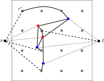
Figure 3: An example flow network for $F$. Crosses signify points in $\mathcal{N}$. Not all edges between $r^{*}$ and $\mathcal{N}^{\circ}$ are shown. Dotted edges have cost 0; dashed edges have cost $\delta\Delta_{\ell}/2$; solid edges have costs given by $\rho_{g}$.

The function $F$ on a vector $x\in\mathbb{R}^{d}$ is the value of a solution of a min-cost flow problem. Let $A_{C}=A\cap C$ and $B_{C}=B\cap C$ be the restriction of input to $C$. For a set of points $A^{\prime}\subseteq A$ we define $\psi(A^{\prime})=\sum_{u\in A^{\prime}}{\psi(u)}$, and we define $\psi(B^{\prime})$ for $B^{\prime}\subseteq B$ analogously. Define $x_{r^{*}}=\psi(A_{C})-\psi(B_{C})-\sum_{r\in\mathcal{N}^{\circ}}{x_{r}}$. For each point $r\in\mathcal{N}$, let $A_{r}=\{u\in A_{C}:N_{\ell}(u)=r\}$ and $B_{r}=\{v\in B_{C}:N_{\ell}(v)=r\}$. We set up an undirected flow network $G_{C}(x)$ as follows. The nodes of the network are $s$, $t$, $\mathcal{N}$, and $A_{C}\cup B_{C}$. $G_{C}$ includes the following edges with corresponding costs:

• $s$ is connected to vertices $A_{C}$ with costs 0, and those vertices $r\in\mathcal{N}$ where $x_{r}<0$, with costs $\delta\Delta_{\ell}/2$;

• $t$ is connected to vertices $B_{C}$ with costs 0, and those vertices $r\in\mathcal{N}$ where $x_{r}>0$, with costs $\delta\Delta_{\ell}/2$;

• any two vertices $u\in A_{C}$ and $v\in B_{C}$ are connected, with cost ${\rho_{g}}(u,v)$;

• any $r\in\mathcal{N}$ is connected to $A_{r}\cup B_{r}$, and the cost of each edge $(r,u)$ is ${\rho_{g}}(r,u)$;

• $r^{*}$ is connected to all $r\in\mathcal{N}^{\circ}$, with corresponding costs ${\rho_{g}}(r^{*},r)$.

An example flow network is shown in Figure 3.

In the following, we use the standard convention $f(u,v)=-f(v,u)$ for any two vertices $u,v$ of $G_{C}(x)$.

Definition 4.5.

The cost function $F(x)$ is defined as the cost of the minimum cost $s$-$t$ flow $f$ from $s$ to $t$ in $G_{C}(x)$, under the constraints:

• $f(s,u)=\psi(u)$ for all $u\in A_{C}$;

• $f(s,r)=-x_{r}$ for all $r\in\mathcal{N}$ for which $x_{r}<0$;

• $f(v,t)=\psi(v)$ for all $v\in B_{C}$;

• $f(r,t)=x_{r}$ for all $r\in\mathcal{N}$ for which $x_{r}>0$;

Above $x_{r^{*}}=x_{r^{*}}=\psi(A_{C})-\psi(B_{C})-\sum_{r\in\mathcal{N}^{\circ}}{x_{r}}$. The function is defined for all $x\in\mathbb{R}^{\mathcal{N}^{\circ}}$

Note that when $x_{r}=0$ for all $r$, and $\psi(A_{C})=\psi(B_{C})$, this flow problem corresponds exactly to the transportation cost problem (1)–(5) with costs given by ${\rho_{g}}$. The interpretation of the arguments is that $x_{r}>0$ means $x_{r}$ demand from $A_{r}$ has to flow to points outside $C$ through $r$ and $x_{r}<0$ means that $-x_{r}$ demand from $B_{r}$ has to flow in from from points outside $C$ through $r$. Having specified all values of $x_{r}$ for $r\in\mathcal{N}^{\circ}$, this leaves an imbalance of $\psi(A_{C})-\psi(B_{C})-\sum_{r\in\mathcal{N}^{\circ}}{x_{r}}$ to flow through $r^{*}$.

We first argue that the flow problem is indeed feasible for all values of $x\in\mathbb{R}^{\mathcal{N}^{\circ}}$.

Lemma 4.6.

For any $x\in\mathbb{R}^{\mathcal{N}^{\circ}}$ and $x_{r^{*}}=\psi(A_{C})-\psi(B_{C})-\sum_{r\in\mathcal{N}^{\circ}}{x_{r}}$, there exists a feasible flow in $G_{C}(x)$ satisfying the constraints of Definition 4.5.

Proof.

We construct a feasible flow $f$ as follows. We set $f(s,u)$, $f(v,t)$ for all $u\in A_{C}$, $v\in B_{C}$ as in Definition 4.5. For each $r\in\mathcal{N}^{\circ}$ we send flow $x_{r}$ from $r^{*}$ to $r$. Then we send $\min\{\psi(A_{C}),\psi(B_{C})\}$ units of flow from $A_{C}$ to $B_{C}$. For each $u\in A\cup B$, let $g(u)$ be equal to the flow going into $u$ minus the flow going out. Moreover, let $g(S)=\sum_{u\in S}{g(u)}$ for any $S\subseteq A_{C}\cup B_{C}$. For each $r\in\mathcal{N}$, send additional flow $g(u)$ from $r$ to each $u\in A_{r}\cup B_{r}$, and flow $g(A_{r})$ from $r^{*}$ to $r$.       

The next argument is the crucial step towards sketching the function $F$. We show that rounding each argument of $F$ to within a small enough multiplicative factor does not change the value of $F$ significantly. The basic reason is that we can lower bound $F(x)$ in terms of $x$, and $F$ is Lipschitz.

Lemma 4.7.

Fix $\epsilon>0$ and suppose $\delta=\epsilon^{O(1)}$. There exists an $\epsilon^{\prime}=\epsilon^{O(1)}$ such that for all feasible $x,x^{\prime}\in\mathbb{R}^{\mathcal{N}^{\circ}}$ satisfying $\forall i:x^{\prime}_{i}/x_{i}\in[1-\epsilon^{\prime},1+\epsilon^{\prime}]$, we have $|F(x)-F(x^{\prime})|\leq\epsilon F(x)$.

Proof.

Observe the following two properties:

• (Lower bound) $F(x)\geq\|x\|_{1}\delta\Delta_{\ell}/2$, because the cost of any edge between $s,t$ and any $r\in\mathcal{N}$ is $\delta\Delta_{\ell}/2$, and each point $r$ in $\mathcal{N}$ either sends flow $x_{r}\geq 0$ to $t$, or receives flow $-x_{r}\geq 0$ from $s$.

• (Lipschitz continuity) for any coordinate $r\in\mathcal{N}$, we have $|F(x+\alpha e_{r})-F(x)|\leq O(\alpha\Delta_{\ell})$, where $e_{r}$ is standard basis vector; for each feasible flow $f$ for $x$, we can create a flow $f^{\prime}$ feasible for $x+\alpha e_{r}$ by setting $f^{\prime}(r,r^{*})=f(r,r^{*})+\alpha$ and $f^{\prime}(s,r),f^{\prime}(t,r),f^{\prime}(s,r^{*}),f^{\prime}(t,r^{*})$ are set as in Definition 4.5; this flow is feasible because in $f^{\prime}$ we have, by Definition 4.5

  $$f^{\prime}(r^{*},s)+f^{\prime}(r^{*},t) =\psi(A_{C})-\psi(B_{C})-\sum_{r\in\mathcal{N}^{\circ}}{x_{r}}-\alpha=f(r^{*},s)+f(r^{*},t)-\alpha$$

  $$f^{\prime}(r,s)+f^{\prime}(r,t) =f(r^{*},s)+f(r^{*},t)+\alpha$$

  Furthermore the difference $f-f^{\prime}$ is nonzero only for edges $(r,r^{*})$, $(r^{*},s)$ and/or $(r^{*},t)$, and $(r,s)$ and/or $(r,t)$; the cost on each of these edges is at most $\Delta_{\ell}/2$ and the change in flow along each edge is at most $\alpha$, which means that the cost of $f^{\prime}$ is at most $O(\alpha\Delta_{\ell})$ larger than the cost of $f$.

Then it follows from the above properties that

$$|F(x^{\prime})-F(x)|\leq\sum_{j}O(\Delta_{\ell})\cdot\epsilon^{\prime}|x_{j}|=O(\epsilon^{\prime}/\delta)\cdot\delta\Delta_{\ell}/2\|x\|_{1}\leq\epsilon F(x),$$

as long as $\epsilon^{\prime}<\gamma\epsilon\delta$ for a sufficiently small constant $\gamma$.       

Lemma 4.8.

Fix $\epsilon>0$ and suppose $\delta=\epsilon^{O(1)}$. For any nonempty cell $C$, there is a sketch $\hat{F}$ for the function $F$ such that for all $x$, $|F(x)-\hat{F}(x)|\leq\epsilon F(x)$, and $\hat{F}$ can be described by a data structure of size $(\log n)^{1/\epsilon^{O(1)}}$.

Proof.

The sketch just remembers $F$ at all points $x$ such that each coordinate $x_{j}$ is of the form $x_{j}=\pm(1+\epsilon^{\prime})^{i}$ for the value of $\epsilon^{\prime}$ guaranteed in Lemma 4.7 and for $i\in[-\log_{1+\epsilon^{\prime}}\epsilon^{-O(1)}\Delta_{L},\log_{1+\epsilon^{\prime}}n]$ . The sketch also remembers the “imbalance”, i.e., $\psi(A_{C})-\psi(B_{C})$. Then, to compute $F(x)$, we construct $x^{\prime}$ by rounding up each coordinate of $x$, and outputing $F(x^{\prime})$. The approximation guarantee follows from Lemma 4.7 if all coordinates $x_{j}$ are larger than $\epsilon\delta^{2}/\Delta_{\ell}$. To finish the proof, we claim that rounding up coordinates that are smaller cannot hurt the approximation factor too much. Each such coordinate can change the value of $F$ by at most $\epsilon\delta^{2}$, and there are less than $\delta^{-2}$ coordinates total, so the total change of value will be at most $\epsilon$. We claim that $F(x)\geq 1$. Indeed, by assumption $C$ is not empty, and the distance between any two points in $A_{C}\cup B_{C}$ is at least one (recall that all points in the input have integer coordinates). It follows that for any arbitrary point $u\in A_{C}\cup B_{C}$, all edges incident to $u$ have cost at least 1, and by the constraints of the flow defining $F$, the total flow outgoing (for $u\in A_{C}$) or incoming (for $u\in B_{C}$) is 1. Therefore, $F(x)\geq 1$, and this finishes the proof.       

4.3 Information Theoretic Algorithm

Suppose we want to compute $F$ for some cell $C$ at level $\ell$. In this section we give a recursive characterization of $F$ in terms of the cost functions of the children of $C$, and we use the characterization to approximate transportation cost with an inefficient algorithm that still satisfies the communication constraints of our model. In the next subsection we will modify this algorithm so that it runs polynomial time.

Let $\{C_{j}\}_{j\in J}$ be the children of $C$, indexed by the set $J$: namely, level $\ell-1$ cells contained in $C$. Let $\{F_{j}\}_{j\in J}$ be the respective cost functions and $\{\hat{F}_{j}\}_{j\in J}$ the corresponding sketches obtained from Lemma 4.8; let $\tau_{j}$ be the imbalance of cell $C_{j}$, i.e.$\tau_{j}=\psi(A_{C_{j}})-\psi(B_{C_{j}})$ (stored in the sketch). Let $\mathcal{N}(C_{j})$ be the full net $\mathcal{N}_{\ell-1}\cap C_{j}$ of $C_{j}$ (of size $1/\delta^{2}$), and let $\mathcal{N}^{\circ}(C_{j})$ be the restricted net. Finally, let $\mathcal{N}$ be the net $C\cap\mathcal{N}_{\ell}$ of $C$ and $\mathcal{N}^{\circ}=\mathcal{N}\setminus R^{*}$ the restricted version. Note that we can pick $c$ and $\delta$ so that for any $R\in\mathcal{N}$, the cluster $\{u:N_{\ell}(u)=R\}$ of points whose closest neighbor is $R$ is a collection of cells $C_{j}$, i.e. $\exists J^{\prime}\subseteq J$ s.t. $\{u:N_{\ell}(u)=R\}\subseteq\bigcup_{j\in J^{\prime}}{C_{j}}$. Then, it follows that for each $C_{j}$ and each $u\in C_{j}$, $N_{\ell}(u)=N_{\ell}(N_{\ell-1}(u))$.

We now define an optimization program used to compute $F$ on some input $z$ using only net points in $\mathcal{N}$, $\mathcal{N}(C_{j})$ for all $j\in J$, and the functions $F_{j}$. For each pair $r\in\mathcal{N}(C_{j}),r^{\prime}\in\mathcal{N}(C_{j^{\prime}})$, where $j,j^{\prime}\in J$, we have a variable $x_{j,r,j^{\prime},r^{\prime}}$, for all $j\neq j^{\prime}$ and $r\in\mathcal{N}(C_{j})$, $r^{\prime}\in\mathcal{N}(C_{j^{\prime}})$. The variable $x_{j,r,j^{\prime},r^{\prime}}$ has the meaning that flow of value $x_{j,r,j^{\prime},r^{\prime}}$ from $A_{C_{j}}\cup B_{C_{j}}$ are is routed to $A_{C_{j^{\prime}}}\cup B_{C_{j^{\prime}}}$, and through $r$ and $r^{\prime}$. By convention, $x_{j,r,j^{\prime},r^{\prime}}=0$ whenever $j=j^{\prime}$. Let $x_{j,r}=\sum_{j^{\prime},r^{\prime}}x_{j,r,j^{\prime},r^{\prime}}$, and $x_{j,\mathcal{N}^{\circ}(C_{j})}$ be the vector $(x_{j,r})_{r\in\mathcal{N}^{\circ}(C_{j})}$.

Another set of variables is $y_{j,r,R}$ for $j\in J$ and $r\in\mathcal{N}(C_{j})$ and $R\in\mathcal{N}$, where $y_{j,r,R}$ stands for the amount of flow from $C_{j}$ routed via $r$ to outside $C$ via the net point $R$. We force that $y_{j,r,R}=0$ except when $R=N_{\ell}(r)$. Also we denote $y_{j,r}=\sum_{R\in\mathcal{N}}y_{j,r,R}$, and let $y_{j,\mathcal{N}^{\circ}(C_{j})}$ be the vector $(y_{j,r})_{r\in\mathcal{N}^{\circ}(C_{j})}$.

Define also the “extra cost” $e_{j,r,j^{\prime},r^{\prime}}$ to be $\rho(r,r^{\prime})-\delta\Delta_{\ell-1}$, and, similarly $e_{j,r,R}=\rho(r,R)-\delta\Delta_{\ell-1}/2$. Note that, because $r,r^{\prime}$ are net points at level $\ell-1$, the value of $e_{j,r,j^{\prime},r^{\prime}}$ and $e_{j,r,R}$ is always non-negative (for $j\neq j^{\prime}$). This is the cost that was unaccounted for by the cost functions $F_{j}$.

The problem is now to minimize the objective

$$\sum_{j}F_{j}(x_{j,\mathcal{N}^{\circ}(C_{j})}+y_{j,\mathcal{N}^{\circ}(C_{j})})+ \sum_{j,j^{\prime}\in J,r\in\mathcal{N}(C_{j}),r^{\prime}\in\mathcal{N}(C_{j^{\prime}})}|x_{j,r,j^{\prime},r^{\prime}}|\cdot e_{j,r,j^{\prime},r^{\prime}}/2$$

$$+ \sum_{j\in J,r\in\mathcal{N}(C_{j}),R\in\mathcal{N}}|y_{j,r,R}|\cdot e_{j,r,R}+\sum_{R\in\mathcal{N}^{\circ}}{(z_{R}\Delta_{\ell}/2+\eta_{R}{\rho_{g}}(R,R^{*}))}$$ (7)

subject to the constraints

$$\sum_{r\in\mathcal{N}(C_{j})}(y_{j,r}+x_{j,r})=\tau_{j}, \forall j\in J$$ (8)

$$x_{j,r,j^{\prime},r^{\prime}}=-x_{j^{\prime},r^{\prime},j,r}, \forall j\in J,j^{\prime}\in J,r\in\mathcal{N}(C_{j}),r^{\prime}\in\mathcal{N}(C_{j^{\prime}})$$ (9)

$$y_{j,r,R}=0 \forall R\neq N_{\ell}(r)$$ (10)

$$\eta_{R}=z_{R}-\sum_{j\in J,r\in\mathcal{N}(C_{j})}y_{j,r,R} \forall R\in\mathcal{N}$$ (11)

$$z_{R^{*}}=\sum_{j\in J}{\tau_{j}}-\sum_{R\in\mathcal{N}^{\circ}}{z_{R}}$$ (12)

$$\eta_{R^{*}}=-\sum_{R\in\mathcal{N}^{\circ}}{\eta_{R}}$$ (13)

Lemma 4.9.

For any $z\in\mathbb{R}^{\mathcal{N}^{\circ}}$, the minimum value of (7) subject to constraints (8)–(13) is equal to $F(z)$.

Proof.

Let $\alpha$ be the optimum achieved by the linear program (7)-(13). We will prove first that $\alpha\geq F(z)$, and then that $\alpha\leq F(z)$.

Clam I: $\alpha\geq F(z)$.

Let $x_{*},y_{*}$ be an optimal solution to the linear program. Also, for each $j\in J$, let $f^{j}$ be the flow achieving optimal cost for $F_{j}(x_{j,\mathcal{N}^{\circ}(C_{j})}+y_{j,\mathcal{N}^{\circ}(C_{j})})$. We will construct a flow $f$ for $F(z)$ achieving cost at most $\alpha$.

To construct $f$, we first construct a flow $f^{\prime}$ in an auxiliary network, defined as follows. The network has vertices $s,t$, $A_{C}\cup B_{C}$ together with $\mathcal{N}\cup\left(\bigcup_{j}\mathcal{N}(C_{j})\right)$, and we will route flow from $s$ to $t$. The edges in the network are defined below:

• $s$ is connected to $A_{C}$, and $t$ is connected to $B_{C}$; all these edges have cost 0;

• $s$ is connected to vertices $R$ in $\mathcal{N}$ for which $z_{R}<0$, and $t$ is connected to vertices $R$ in $\mathcal{N}$ for which $z_{R}>0$; each of these edges has cost $\delta\Delta_{\ell}/2$

• the network induced on $A_{C_{j}}\cup B_{C_{j}}\cup\mathcal{N}(C_{j})$ is identical to the network defining $F_{j}$, (with $s$, $t$ and their incident edges removed); the costs are also identical as in the definition of $F_{j}$;

• we have the complete graph on $\bigcup_{j}{\mathcal{N}(C_{j})}$; edges between points $r\in\mathcal{N}(C_{j})$ and $r^{\prime}\in\mathcal{N}(C_{j^{\prime}})$ have cost $\rho(r,r^{\prime})$

• each $r\in\mathcal{N}(C_{j})$ for some $j$ is connected to $N_{\ell}(r)\in\mathcal{N}$ at cost ${\rho_{g}}(r,N_{\ell}(r))$; also each $R\in\mathcal{N}^{\circ}$ is connected to $R^{*}$ at cost ${\rho_{g}}(R,R^{*})$.

The flow $f^{\prime}$ between $s$, $t$, and their neighbors is defined similarly to the flow problem defining $F$. We route flow $f^{\prime}(s,u)=1$ from $s$ to each $u\in A_{C}$ and flow $f(v,t)=1$ from each $v\in B_{C}$ to $t$. We also route flow $f(R,t)=z_{R}$ from each $R\in\mathcal{N}$ for which $z_{R}>0$ to $t$; similarly, we route flow $f(s,R)=-z_{R}$ for each $R\in\mathcal{N}$ for which $z_{R}<0$.

We define the rest of $f^{\prime}$ based on $x_{*},y_{*},f^{j}$. The flow restricted to the network induced by $A_{C_{j}},B_{C_{j}},\mathcal{N}(C_{j})$ for each $j$ is exactly as in $f^{j}$. For each $u\in A_{C}$, $f^{\prime}(s,u)=\psi(u)$, and for each $v\in B_{C}$, $f^{\prime}(v,t)=\psi(v)$. For each $r\in\mathcal{N}(C_{j}),r^{\prime}\in\mathcal{N}(C_{j^{\prime}})$ for $j\neq j^{\prime}$, we set $f^{\prime}(r,r^{\prime})=x_{j,r,j^{\prime},r^{\prime}}$. For each $r\in\mathcal{N}(C_{j}),R\in\mathcal{N}$, we set $f^{\prime}(r,R)=y_{j,r,R}$. For each $R\in\mathcal{N}^{\circ}$, we set $f^{\prime}(R^{*},R)=\eta_{R}$.

We claim that flow conservation is satisfied for $f^{\prime}$. This is immediate for each $u\in A_{C}$ and each $v\in B_{C}$, by the feasibility of each $f^{j}$. By the constraints of $f^{j}$, each $r\in\mathcal{N}^{\circ}(C_{j})$ has incoming flow $x_{j,r}+y_{j,r}$, and by the construction of $f^{\prime}$ and (9) this is also the outgoing flow. By (8), the total flow leaving $r_{j}^{*}$ is $\tau_{j}-\sum_{r\in\mathcal{N}^{\circ}(C_{j})}{(x_{j,r}+y_{j,r})}$, which, by the constraints of $f^{j}$ is the incoming flow as well. Flow conservation can be verified for $R\in\mathcal{N}$ using (11)-(13).

Next we claim that the cost of $f^{\prime}$ is $\alpha$. For any $j$, the flow and flow costs on edges in the network induced on $A_{C_{j}}$, $B_{C_{j}}$, $\mathcal{N}(C_{j})$ are exactly as in $f^{j}$; the total cost on these edge is

$$F_{j}(x_{j,\mathcal{N}^{\circ}(C_{j})}+y_{j,\mathcal{N}^{\circ}(C_{j})})-\sum_{r\in\mathcal{N}(C_{j})}{(x_{j,r}+y_{j,r})\delta\Delta_{\ell-1}/2}.$$

The cost of flow $f^{\prime}$ along edges $(r,r^{\prime})$, $r\in\mathcal{N}(C_{j})$, $r^{\prime}\in\mathcal{N}(C_{j^{\prime}})$ as well as that along edges $(r,R)$, $r\in\mathcal{N}(C_{j}),R\in\mathcal{N}$ contribute $\sum_{r\in\mathcal{N}(C_{j})}{(x_{j,r}+y_{j,r})\delta\Delta_{\ell-1}/2}$ plus the second and third term of (7). The fourth term of (7) is given by the cost of the flow between $s$, $t$, and $\mathcal{N}$ together with the cost of the flow between $R^{*}$ and $R\in\mathcal{N}^{\circ}$.

We are now ready to define $f$ based on $f^{\prime}$. Since $f^{\prime}$ is a feasible flow, it can be decomposed into flows $f^{\prime}_{1},\ldots,f^{\prime}_{k}$, where each $f^{\prime}_{i}$ is supported on an $s$-$t$ path. For each $u\in A$, $v\in B$, the flow $f(u,v)$ is defined as the sum of flows $f^{\prime}_{i}$ along paths that pass from $s$ to $u$ to $v$ to $t$. Similarly, the flow $f(u,R)$ is defined as the sum of flows $f^{\prime}_{i}$ along paths that pass through both $u$ and $R$. Finally, $f(R,R^{*})=f^{\prime}(R,R^{*})$, $f(s,R)=f^{\prime}(s,R)$, and $f(R,t)=f^{\prime}(R,t)$ for each $R\in\mathcal{N}$. This specifies $f$.

To complete the proof of the claim we need to show that the cost of $f$ is at most the cost of $f^{\prime}$. Edges between $s$, $t$, and points in $\mathcal{N}$, as well as for edges between $R^{*}$ and points in $\mathcal{N}^{\circ}$ exist both in the network defining $f^{\prime}$ and the network defining $f$, and they have identical flow and cost. Then, it remains to show that for $u,v\in A_{C}\cup B_{C}$, the cost of a unit of flow in $f^{\prime}$ routed along a path that goes from $u$ to $v$ is at least ${\rho_{g}}(u,v)$. When $u,v\in C_{j}$, this follows from the triangle inequality for ${\rho_{g}}$. It then suffices to show the claim for a path consisting of edges $(u,r)$, $(r,r^{\prime})$, and $(r^{\prime},v)$, where $u\in C_{j}$, $r=N_{\ell-1}(u)$, $v\in C_{j^{\prime}}$ ($j\neq j^{\prime})$, and $r^{\prime}=N_{\ell-1}(v)$; any other path consists of such segments and paths that are entirely within a cell $C_{j}$. But, by the definition of ${\rho_{g}}$, since $\ell-1$ is the highest level at which $u$ and $v$ are separated, ${\rho_{g}}(u,v)=\rho(r,r^{\prime})+{\rho_{g}}(u,r)+{\rho_{g}}(v,r)$, and the right hand side of this identity is exactly the cost of a unit flow of $f^{\prime}$ along the path $\{(u,r),(r,r^{\prime}),(r^{\prime},v)\}$. An analogous argument shows that the cost of a unit of flow in $f^{\prime}$ routed along a path that goes from $u\in A\cup B$ to $R\in\mathcal{N}$ is at most ${\rho_{g}}(u,R)$, and, together with the triangle inequality for ${\rho_{g}}$, this completes the proof that the cost of $f$ is at most the cost of $f^{\prime}$. Since the cost of $f^{\prime}$ is at most $\alpha$, and $f$ is a feasible flow satisfying the constraints of Definition 4.5, it follows that $F(z)\leq\alpha$.

Clam II: $\alpha\leq F(z)$.

To prove that $\alpha\leq F(z)$, we will use a flow $f$ of cost $F(z)$, feasible for Definition 4.5, and construct a solution $y_{*},x_{*},\eta_{*}$ for the LP (7)-(13), as well as flows $f^{j}$ for $F_{j}$ for each $j$, so that the objective (7) is at most the cost of $f$. For any $u,v\in C_{j}$, we set $f^{j}(u,v)=f(u,v)$. Then, for $u\in C_{j}$, $r=N_{\ell-1}(u)$, and $R=N_{\ell}(u)=N_{\ell}(r)$, we set

$$f^{j}(u,r)=f(u,R)+\sum_{v\in C_{j^{\prime}},j^{\prime}\neq j}{f(u,v)}.$$

This defines all $f^{j}$, and also $x_{j,\mathcal{N}^{\circ}(C_{j})}$. We then set

$$x_{j,r,j^{\prime},r^{\prime}}=\sum_{u\in A_{r},v\in B_{r}}{f(u,v)}\hskip 12.91663pt\text{ and }\hskip 12.91663pty_{j,r,R}=\sum_{u\in A_{r}\cup B_{r}}{f(u,R)}.$$

Finally, let $\eta_{R}=f(R^{*},R)$. The flow conservation inequalities for $f$ imply the feasibility of $f^{j}$ for each $j$, as well as (8)-(13). The total of (7) and the costs of $f^{j}$ is equal to the cost of $f$, by the definition of distance function ${\rho_{g}}$.       

In order to satisfy the space and communication requirements of our model,we cannot represent the function $F_{j}$ exactly, and instead we replace each $F_{j}$ with the sketch $\hat{F}_{j}$. Thus, we consider the optimization problem with objective function

$$\sum_{j}\hat{F}_{j}(x_{j,\mathcal{N}^{\circ}(C_{j})}+y_{j,\mathcal{N}^{\circ}(C_{j})})+ \sum_{j,j^{\prime}\in J,r\in\mathcal{N}(C_{j}),r^{\prime}\in\mathcal{N}(C_{j^{\prime}})}|x_{j,r,j^{\prime},r^{\prime}}|\cdot e_{j,r,j^{\prime},r^{\prime}}/2$$

$$+ \sum_{j\in J,r\in\mathcal{N}(C_{j}),R\in\mathcal{N}}|y_{j,r,R}|\cdot e_{j,r,R}+\sum_{R\in\mathcal{N}^{\circ}}{(z_{R}\Delta_{\ell}/2+\eta_{R}{\rho_{g}}(R,R^{*}))}$$ (14)

subject to (8)-(13), where $\hat{F}_{j}$ is a sketch of $F_{j}$.

Next we define an inefficient unit step that satisfies the space and communication constraints of the MPC model. In the following subsection we also give a polynomial time variant of the unit step.

Unit Step (information theoretic).

The (inefficient) unit step $\mathcal{A}_{i}$, when executed in cell $C$ at level $\ell$, accepts as input all the sketches $\hat{F}_{j}$ for all children $C_{j}$ of $C$ (if $\ell=1$, we assume we have $F_{j}$ exactly). It solves (14) on all inputs $z\in\mathbb{R}^{\mathcal{N}^{\circ}}$ for which $z_{i}=\pm(1+\epsilon^{\prime})^{j_{i}}$ where $j_{i}$ is an integer in $[-\log_{1+\epsilon^{\prime}}\epsilon^{-O(1)}\Delta_{L},\log_{1+\epsilon^{\prime}}n]$ and $\epsilon^{\prime}$ is as in Lemma 4.8. It then outputs the computed objective values and the cell imbalance $\psi(A_{C})-\psi(B_{C})$ as the sketch $\hat{F}$ for $F$.

Theorem 4.10.

The unit step $\mathcal{A}_{i}$ has space complexity $s_{u}(n_{u})=O(n_{u}^{2})$ and output size $p_{u}=(\log n)^{\epsilon^{-O(1)}}$. Moreover, the Solve-and-Sketch algorithm with unit step $\mathcal{A}_{i}$ that outputs (14) with $z=(0,\ldots,0)$ in the unique cell $C\in P_{L}$ containing $A\cup B$, computes an $1\pm O(L\epsilon)$ approximation to $\operatorname{cost}(A,B,\psi)$.

Proof.

Observe that $F(0,\ldots,0)=\operatorname{cost}_{\rho_{g}}(A,B,\psi)$. By Lemma 4.4, it is then enough to prove that for all cells $C$ on level $\ell$, and for each $x\in\mathbb{R}^{\mathcal{N}^{\circ}}$, the value computed by (14) is a $(1\pm O(\ell\epsilon))$ approximation of $F(x)$. For $\ell=1$, this is immediate because we compute the exact value of $F$. For $\ell>1$ the claim follows by induction from Lemmas 4.9, 4.8, because each term of (7) is non-negative.       

4.4 Computationally Efficient Algorithm

The goal in this section is to show that (a variant of) the unit step from the previous section can be implemented in polynomial time. Then the existence of an efficient MPC algorithm for approximating transportation cost will follow from Theorem 4.10.

As before, we fix a cell $C$ on level $\ell$ and focus on approximating $F$ evaluated in the cell. We first observe that the function $F$ is convex in its parameters. Then we use this fact to show that a “convexification” of the sketch $\hat{F}$ is also an accurate approximation to $F$. The two lemmas follow.

Lemma 4.11.

For any cell $C$ the associated function $F$ is convex.

Proof.

Consider any $x,y\in\mathbb{R}^{d}$. Consider $F(x)$ and suppose $f^{x}$ is the minimum cost flow for $F(x)$. Similarly, suppose $f^{y}$ is the minimum cost flow for $F(y)$. Then, note that $\frac{f^{x}+f^{y}}{2}$ is a feasible solution to $F(\frac{x+y}{2})$, and achieves a value of $\frac{F(x)+F(y)}{2}$ (by linearity). Since there could be other, lower cost solutions to $F(\frac{x+y}{2})$, we conclude that $F(\frac{x+y}{2})\leq\frac{F(x)+F(y)}{2}$.       

Lemma 4.12.

Let $\epsilon^{\prime}$ be as in Lemma 4.8. Let $X$ be the matrix whose columns are all points $x\in[-n,n]^{d}$ such that for all $i\in[d]$, $x_{i}=\pm(1+\epsilon^{\prime})^{j_{i}}$ for some integer $j_{i}\in[-\log_{1+\epsilon^{\prime}}\epsilon^{-O(1)}d\Delta_{L},\log_{1+\epsilon^{\prime}}n]$. Let $f$ be the vector defined by $f_{i}=F(x^{i})$, where $x^{i}$ is the $i$-th column of $X$. Then the function $\tilde{F}$ defined by

$$\tilde{F}(x)=\min\{\sum_{i}\alpha_{i}f_{i}:x=X\alpha,\ \alpha\geq 0,\ \sum_{i}\alpha_{i}=1\},$$

satisfies

$$|F(x)-\tilde{F}(x)|\leq\epsilon F(x).$$

Proof.

We first use the convexity of $F$ to prove that $\tilde{F}(x)\geq F(x)$. For this, it is enough to observe that for any $\alpha\geq 0$, such that $\sum_{i}\alpha_{i}=1$, we have $F(X\alpha)\leq\sum_{i}{\alpha_{i}F(x^{i})}$ by Lemma 4.11, and in particular this holds for the minimizer $\alpha$ that gives $\tilde{F}(x)$.

Next we show that $\tilde{F}(x)\leq(1+\epsilon)F(x)$. Fix some $x$, and let, for each $j\in[d]$, $k_{j}$ be $k_{j}=\lfloor\log_{1+\epsilon^{\prime}}|x_{j}|\rfloor$, and $s_{j}$ be $1$ if $x_{j}>0$, and $-1$ otherwise. Then $x$ is in the convex hull of the points $S(x)=\{(s_{1}(1+\epsilon^{\prime})^{k_{1}+b_{1}},\ldots,s_{d}(1+\epsilon^{\prime})^{k_{d}+b_{d}}):\forall j:b_{j}\in\{0,1\}\}$. Therefore, $\tilde{F}(x)\leq\max\{F(x^{\prime}):x^{\prime}\in S(x)\}$. But, by Lemma 4.7, $\max\{F(x^{\prime}):x^{\prime}\in S(x)\}\leq(1+\epsilon)F(x)$, and the claim follows.       

The crucial property of $\tilde{F}$ is that it is specified as a solution to a linear program, and as such it’s easy to “embed” inside a larger linear program. We do this for the program (7)-(13) next.

Let $X$ be as in Lemma 4.12 and $D$ be the number of columns of $X$. Observe that $D=(\log n)^{\epsilon^{-O(1)}}$. Let, for each $j\in J$, $f^{j}$ be a vector of dimension $D$, such that $f^{j}_{i}=F_{j}(x^{i})$, for $x^{i}$ the $i$-th column of $X$. We consider the linear program whose objective is to minimize:

$$\sum_{j}\langle f^{j},\alpha^{j}\rangle+ \sum_{j,j^{\prime}\in J,r\in\mathcal{N}(C_{j}),r^{\prime}\in\mathcal{N}(C_{j^{\prime}})}|x_{j,r,j^{\prime},r^{\prime}}|\cdot e_{j,r,j^{\prime},r^{\prime}}/2$$

$$+ \sum_{j\in J,r\in\mathcal{N}(C_{j}),R\in\mathcal{N}}|y_{j,r,R}|\cdot e_{j,r,R}+\sum_{R\in\mathcal{N}^{\circ}}{(z_{R}\Delta_{\ell}/2+\eta_{R}{\rho_{g}}(R,R^{*}))}$$ (15)

subject to constraints (8)-(13) as well as the additional constraints:

$$x_{j,\mathcal{N}^{\circ}(C_{j})}+y_{j,\mathcal{N}^{\circ}(C_{j})}=X\alpha^{j} \forall j\in J$$ (16)

Unit Step (efficient).

The (efficient) unit step $\mathcal{A}_{e}$, when executed in a cell $C$ (with net $\mathcal{N}$ inside the cell, and restricted net $\mathcal{N}^{\circ}=\mathcal{N}\setminus\{R^{*}\}$) on level $\ell>1$, takes as input the vectors $f^{j}$ for all child cells $C_{j}$, as well as the imbalances $\tau_{j}$. It solves (15) on all inputs $z\in\mathbb{R}^{\mathcal{N}^{\circ}}$ for which $z_{i}=\pm(1+\epsilon^{\prime})^{j_{i}}$ where $j_{i}$ is an integer in $[-\log_{1+\epsilon^{\prime}}\epsilon^{-O(1)}\Delta_{L},\log_{1+\epsilon^{\prime}}n]$ and $\epsilon^{\prime}$ is as in Lemma 4.8 and outputs the computed objective value for each input to form a vector $f$. It also outputs the cell imbalance $\psi(A_{C})-\psi(B_{C})$. At level $\ell=1$, the function $F$ is evaluated exactly.

Theorem 4.13.

The unit step $\mathcal{A}_{eu}$ has polynomial space and time complexity (i.e. $s_{u}(n_{u}),t_{u}(n_{u})=n_{u}^{O(1)}$) and output size $p_{u}=(\log n)^{\epsilon^{-O(1)}}$. Moreover, the solve-and-sketch algorithm with unit step $\mathcal{A}_{i}$ that outputs (15) with $z=(0,\ldots,0)$ in the unique cell $C\in P_{L}$ containing $A\cup B$, computes an $1\pm O(L\epsilon)$ approximation to $\operatorname{cost}(A,B,\psi)$.

Proof.

The proof of approximation is analogous to the proof of Theorem 4.10, but using Lemma 4.12 rather than Lemma 4.8. The space and time complexity claims follow since(15) is a equivalent to a linear optimization problem and can be solved in polynomial time and space.       

We now deduce Theorem 4.1, from Theorem 4.13 (with $\epsilon^{\prime}=O(\epsilon/L)=O(\epsilon/\log_{s}n)$) and Theorem 2.1.

4.5 Consequences

Theorem 4.13 has consequences beyond the MPC model: it implies a near linear time algorithm and an algorithm in the streaming with sorting routine model for EMD and the transportation problem.

The first theorem follows directly from the simulation of MPC algorithms by algorithms in the streaming with sorting routine model.

Theorem 4.14.

Let $\epsilon>0$, and $s\geq(\log n)^{(\epsilon^{-1}\log_{s}n)^{O(1)}}$. Then there a space $s$ algorithm that runs in $(\log_{s}n)^{O(1)}$ rounds in the streaming with sorting routine model, and, on input sets $A,B\subseteq\mathbb{R}^{2}$, $|A|+|B|=n$, and demand function $\psi:A\cup B\rightarrow\mathbb{N}$ such that $\sum_{u\in A}\psi(u)=\sum_{b\in B}\psi(v)$ outputs a $1+\epsilon$ approximation to $\operatorname{cost}(A,B,\psi)$.

The existence of a nearly-linear time algorithm for EMD and the transportation problem also follows easily from Theorem 4.13. We stated this result as Theorem 4.2, and we prove it next.

Proof of Theorem 4.2.

The algorithm simulates the Solve-And-Sketch algorithm sequentially, by applying the unit step $\mathcal{A}_{eu}$ with approximation parameter $\epsilon^{\prime}=\epsilon/L$ to each (non-empty) cell at level $\ell=1,\ldots,L$ of the partition, and finally outputs (15) with $z=(0,\ldots,0)$. We choose the branching factor $c$ of the hierarchical partition to be $(\log n)^{\omega(1)}$, so that the size of the output of $\mathcal{A}_{eu}$ is $n^{o(1)}$, and the height $L$ of the partition is $L=o(\log n)$. The running time bound follows.       

5 Parallel Implementation of the Solve-And-Sketch Framework

In this section we describe how to implement in the MPC model algorithms that fit the Solve-And-Sketch framework. In particular, we prove Theorem 2.1 from Section 2. In fact it will follow from a more general Theorem 5.2 below. Both theorems assume the existence of a unit step algorithm $\mathcal{A}_{u}$.

Consider a hierarchical partition $P=(P_{0},\ldots,P_{L})$ of an input pointset $S$, where $P_{\ell-1}$ is a subdivision of $P_{\ell}$ for each $\ell$. Recall that the children of a cell $C\in P_{\ell}$ are subcells $C^{\prime}\in P_{\ell-1}:C^{\prime}\subseteq C$, and the degree of $P$ is the maximum number of children any cell $C$ has. (For simplicity, think of these parameters as $L=O(1)$ and $c=s^{1/3}$.) In order to implement our algorithms, we require that each point $u$ in the input is labeled by the sequence $(C_{0}(u),\ldots,C_{L}(u))$, where $C_{\ell}(u)\in P_{\ell}$ is the unique cell on level $\ell$ the partition that contains $u$. When the input $S$ is represented in this way, we say that it is labeled by $P$. In this section we discuss in detail how to label subsets of Euclidean space; the corresponding construction for arbitrary metric spaces of bounded doubling dimension is discussed in Section 6.

We assume that we have a total ordering on all cells with the following property:

• (Hierarchical property.) For any $\ell\in\{1,\ldots,L\}$, and any two cells $C_{1},C_{2}\in P_{\ell}$, $C_{1}<C_{2}$ implies that for any child $C^{\prime}_{1}$ of $C_{1}$ and any child $C^{\prime}_{2}$ of $C^{\prime}_{2}$, $C^{\prime}_{1}<C^{\prime}_{2}$.

We call an ordering with the above property a good ordering.

In each round of the algorithm, we sort all cells which have not yet been processed and we assign an interval of cells to a machine. Using the bound $L$ on the number of levels of the partition and the degree bound $c$, we show that after each machine recursively applies the unit step to each of its assigned cells, the output to the next round of computation is significantly smaller than the input to the current round. This enables bounding the total number of rounds by essentially $(\log_{s}n)^{O(1)}$ (for good choices of $L$ and $c$).

We give the implementation of the Solve-And-Sketch algorithm in the MPC model as Algorithm 2.

input : A set $S$, labeled by a hierarchical partition $P=(P_{0},\ldots,P_{L})$ of degree $c$ such that $P_{0}$ is a partition into singletons.

1

2for $r=1,\ldots R$ do

3      

4      Let $\mathcal{C}_{r}$ be the be the set of non-empty cells $C$ of $P$ such that (1) $C\in P_{0}$ or the unit step $\mathcal{A}_{u}$ has already been applied to $C$, and (2) the unit step has not been applied to the parent of $C$.

5       Sort $\mathcal{C}_{r}$ according to the induced order. Let the sorted order be $C_{1},\ldots,C_{n_{r}}$.

6      

7      Let $p_{u}(C_{i})$ be the output size of cell $C_{i}$. Compute $h_{i}=\sum_{j\leq i}p_{u}(C_{j})$ for all $i\leq n_{r}$ using a prefix sum algorithm.

8      

9      Consider some cell $i$, and let $j=\lceil\frac{h_{i}}{s}\rceil$. Machine $j$ receives the output of the unit step that has been applied in round $r-1$ to $C_{i}$.

10      

11      foreach machine $j$ do

12             for $\ell=1,\ldots,L$ do

13                   while there exists a cell $C\in P_{\ell}$ such that $C\subseteq\bigcup_{i:(j-1)s\leq h_{i}<js}{C_{i}}$ do

14                        

15                        Apply the unit step $\mathcal{A}_{u}$ to $C$, where the inputs are: for $\ell>1$: the outputs of the unit step for children of $C$ for $\ell=1$: the cells that are children of $C$

16                         (If the output of $\mathcal{A}_{u}$ is larger than its input size, the algorithm instead just outputs the input; appropriately marked to be “lazy evaluated”.)

17                  

18            

19      

Algorithm 2 Implementation of algorithms in the Solve-And-Sketch framework

For two cells $C_{1}\in P_{\ell_{1}}$, $C_{2}\in P_{\ell_{2}}$, let $[C_{1},C_{2}]=\{C:C_{1}\leq C\leq C_{2}\}$. We call a cell $C\in[C_{1},C_{2}]$ a boundary cell if there exists a sibling $C^{\prime}$ of $C$ such that $C^{\prime}\not\in[C_{1},C_{2}]$.

The following lemma bounds the number of boundary cells for any interval $[C_{1},C_{2}]$, and is key to the analysis of Algorithm 2.

Lemma 5.1.

For a partition $P=(P_{0},\ldots,P_{L})$ and a range $[C_{1},C_{2}]$, the number of boundary cells is at most $2(c-1)L$.

Proof.

It suffices to show that there are at most $2c-2$ boundary cells in each level $\ell\in\{0,\ldots,L-1\}$. Indeed, suppose for the sake of contradiction that there are $n_{\ell}>2c-2$ boundary cells in $P_{\ell}$: call the set of such sets $\mathcal{C}$, and number them as $C_{1}\leq C^{\ell}_{1}<C^{\ell}_{2}<\dots<C^{\ell}_{n_{\ell}}\leq C_{2}$. Then there must be at least three cells $C_{1}^{\ell+1}<C_{2}^{\ell+1}<C_{3}^{\ell+1}$ ($C_{1}^{\ell+1},C_{2}^{\ell+1},C_{3}^{\ell+1}\in P_{\ell+1}$), such that each of them has at least one child cell in $\mathcal{C}$. But by the hiearchical property of good orderings, this implies that for all children $C$ of $C_{2}$, $C_{1}\leq C_{1}^{\ell}<C<C^{\ell}_{n_{\ell}}\leq C_{2}$, and therefore none of the children of $C_{2}^{\ell+1}$ is a boundary cell, a contradiction.       

Theorem 5.2.

Let $P$ be a hierarchical partition of the input $S$, and let $S$ be labeled by $P$. Furthermore, let $\mathcal{A}_{u}$ be a unit step algorithm, which, for input of size $n_{u}$, has time $t_{u}=t_{u}(n_{u})$ and space $s_{u}=s_{u}(n_{u})$, as well as parameter $p_{u}=p_{u}(n_{u})$. Assume all functions are non-decreasing, and let $p_{u}=p_{u}(s),t_{u}=t_{u}(cp_{u})$. Suppose $s_{u}(cp_{u})\leq s$, and $p_{u}(s)\leq\tfrac{\sqrt{s}}{4cL}$.

Algorithm 2 can be simulated using $R\cdot O(\log_{s}n)$ rounds in the MPC model. Furthermore, after $R=O(\log_{s}n)$ rounds, Algorithm 2 has applied the unit step to all cells of the hierarchical partition $P$. If comparing two cells in some good ordering requires time $\tau$, then the local computation time per machine in a round is bounded by $O(s\cdot(\tau\cdot\log s\cdot\log_{s}n+Lt_{u}))$. All bounds are with high probability.

Proof.

We first show that each iteration of the loop in Step 2 can be computed in $O(\log_{s}n)$ rounds of the MPC model with high probability. To that end, we use the sorting algorithm and the prefix-sum algorithm of Goodrich et al. [GSZ11], which obtains this bound with high probability, because they operate on input of size $n_{r}=|\mathcal{C}_{r}|\leq n$. The other steps of each iteration can easily be simulated in a constant number of rounds.

Now we bound the number of rounds $R$ before the unit step has been applied to all cells of $P$. In round $r$, machine $j$ takes a range $[C_{i_{j}},C_{i_{j+1}-1}]$ where $i_{j}$ are determined from the prefix-sum calculation.

Let $\mathcal{C}_{r+1,j}$ be the cells $C$ such that

• machine $j$ applies the unit step to $C$ in round $r$,

• the unit step is not applied to the parent of $C$ in round $r$.

All such cells are boundary cells, and by Lemma 5.1, $|\mathcal{C}_{r+1,j}|\leq cL$; since $\mathcal{C}_{r+1}=\bigcup_{j}{\mathcal{C}_{r+1,j}}$, we have $n_{r+1}\leq cL\lceil\tfrac{n_{r}}{s/p_{u}-1}\rceil$ (in each machine, there are at least $s/p_{u}-1$ distinct outputs that are processed, i.e., “consumed”). Since $p_{u}\leq\tfrac{\sqrt{s}}{4cL}$, we have that $n_{r+1}\leq n_{r}/\sqrt{s}$, i.e., there can be only $R=\log_{\sqrt{s}}n=O(\log_{s}n)$ rounds before $\mathcal{C}_{r}$ fits entirely on a machine. Once $\mathcal{C}_{r}$ fits on a single machine, the process finishes.

In terms of space and computation, each machine always receives at most $O(s)$ amount of information, by construction. Furthermore, because of lazy evaluation, the output is always no larger than the input for any fixed machine $j$. Hence, we also never run out of machines when partitioning $C_{i}$’s outputs (namely, the total “information” in the system remains bounded by $O(n)$, in chunks of size at most $p_{u}\leq s$). Finally, the space is bounded by the machine input size, $O(s)$, plus local space required by $\mathcal{A}_{u}$, which is $s_{u}(cp_{u})\leq s$ since $cp_{u}\leq s$ is the bound on the input into a unit step.

Finally, we bound the computation time per machine. The sorting/prefix-sum parts take time $O(s\tau_{1}\cdot\log s\cdot\log_{s}n)$. The rest of the computation time is dominated by the worst-case unit step computation. Overall, no more than $O(sLt_{u})$ computation per machine is necessary in a single iteration of the loop in Step 2, once we are done with sorting.       

We remark that the above theorem immediately implies Theorem 2.1.

Proof of Theorem 2.1.

Suppose $s_{u}(n_{u}),t_{u}(n_{u})$ are all bounded by the polynomial $(n_{u})^{q}$, where $q\geq 1$ is constant. Fix $c=s^{1/(2q)}$. Then we get that $L=\tfrac{\log\Delta}{c^{1/d}}=O(d\log_{s}n)$.

We verify we can apply Theorem 5.2. Indeed, we have that $p_{u}=p_{u}(s)\leq s^{1/3}\leq\tfrac{\sqrt{s}}{4cL}$. We also have $s_{u}(cp_{u}(s))\leq(cp_{u}(s))^{q}\leq c^{q}\cdot p_{u}(s)^{q}\leq\sqrt{s}\cdot s^{1/3}<s$. The theorem follows.       

5.1 Constructing a Partition in the Euclidean Space

We now describe how an $(a,b,c)$-partition can be computed for the Euclidean space in MPC. This is an elaboration on the construction described in Section 2, and is used for our Euclidean MST and transportation cost algorithms.

Lemma 5.3.

Let $a>1$, $d$, and $L$ be positive integers. Consider a metric space $(S,\ell_{2}^{d})$, where $S\subseteq\mathbb{R}^{d}$, $|S|=n$. There is a $(1/a,d,(a+1)^{d})$-distance-preserving partition $\mathcal{P}$ of $S$ with approximation $\gamma\leq\sqrt{d}$ and $L+1$ levels. Moreover $S$ can be labeled by a hierchical partition $P$ sampled from $\mathcal{P}$ in $O(\log_{s}n)$ rounds of MPC, and $P$ has a good ordering of subcells such that each pair of cells can be compared in $O(dL)$ time.

Proof.

The partition is constructed by applying a randomly shifted grid, similarly to Arora’s classical construction [Aro98]. Let us shift $S$ so that for all $u\in S$, and all coordinates $i\in[d]$, $u_{i}\geq 0$, and also there exists a $v\in S$ and a coordinate $i$ such that $v_{i}=0$. Let, further, $\Delta$ be the smallest real number such that $S\subseteq[0,\Delta]^{d}$. A point $r$ is selected uniformly at random from $[0,\Delta]^{d}$. Two points $u$ and $v$ belong to the same cell at level $\ell\in\{0,\ldots,L\}$ if and only if for all dimensions $i\in[d]$, $\left\lfloor\frac{(u_{i}-r_{i})a^{L-\ell}}{\Delta}\right\rfloor=\left\lfloor\frac{(v_{i}-r_{i})a^{L-\ell}}{\Delta}\right\rfloor$.

Let us state the desired properties of the partition.

1. The diameter of a cell at level $\ell$ is bounded by $\Delta_{\ell}=\sqrt{d}\Delta/a^{L-\ell}$; moreover, by the choice of $\Delta$, $\operatorname{diam}(S)=\max_{u,v\in S}{\|u-v\|_{2}}\geq\max_{u,v\in S}{\|u-v\|_{\infty}}=\Delta$.

2. Consider two points $u,v\in H$. The probability that $\left\lfloor\frac{(u_{i}-r_{i})a^{L-\ell}}{\Delta}\right\rfloor\neq\left\lfloor\frac{(v_{i}-r_{i})a^{L-\ell}}{\Delta}\right\rfloor$ for a given $i$ is at most $\frac{|u_{i}-v_{i}|a^{L-\ell}}{\Delta}$. Therefore, by the union bound, the probability that $u$ and $v$ belong to different cells is bounded by

   $$\frac{\|u-v\|_{1}a^{L-\ell}}{\Delta}=\sqrt{d}\cdot\frac{\|u-v\|_{1}}{\sqrt{d}\Delta/a^{L-\ell}}\leq d\cdot\frac{\|u-v\|_{2}}{\Delta_{\ell}},$$

   where the last inequality follows from the inequality $\|x\|_{1}\leq\sqrt{d}\|x\|_{2}$, which holds for any $x$.

3. The degree of the cell containing all points is bounded by $(a+1)^{d}$. The degree of subcells is bounded by $a^{d}$.

To label the set $S$ by a hierarchical partition, sampled as above, we need to first shift $S$ and compute $\Delta$ so that $S\subseteq[0,\Delta]^{d}$ as above. For this, we just need to compute the smallest and largest coordinate of any point in $S$, which can be done in $O(\log_{s}n)$ rounds of MPC. Then, to label each $u\in S$, we let an arbitrary processor sample $r$ and broadcast it to all other processors; for each $\ell$, $u$ is labelled by the sequence $\left(\left\lfloor\frac{(u_{i}-r_{i})a^{L-\ell}}{\Delta}\right\rfloor\right)_{i=1}^{d}$, which uniquely identifies $C_{\ell}(u)$.

Next we define one notion of a good ordering. To compare two cells $C_{1},C_{2}$, we find the lowest $\ell$ for which they belong to the same cell $C\in P_{\ell}$. If $C_{1}\in P_{\ell}$, then $C_{1}<C_{2}$, and vice versa. Otherwise if $C_{1},C_{2}\not\in P_{\ell}$, we consider the two cells $C^{\prime},C^{\prime\prime}\in P_{\ell-1}$ such that $C_{1}\subseteq C^{\prime}$ and $C_{2}\subseteq C^{\prime\prime}$. If the centroid of $C^{\prime}$ precedes the centroid of $C^{\prime\prime}$ lexigraphically, then $C_{1}<C_{2}$, and vice versa. This ordering can be seen as a pre-order on the natural tree structure associated with $P$, where the children of each node are ordered lexicographically. It is straightforward to verify that the hierarchical property is satisfied. Two cells, represented by their centroids and level $\ell$ can be compared in $O(dL)$ time.       

5.2 Bounded Ratio for MST and EMD

We now show why we can assume that our dataset has a bounded ratio in the MST and EMD applications. In particular, we show how to reduce an arbitrary dataset to one where the aspect ratio is bounded by a polynomial in $n$, while incurring a multiplicative error of $1+\epsilon$ only. To be precise, we note that we assume that original points are from a set $[0,\Delta]^{d}$, where the machine word size is $O(\log\Delta)$.

We employ standard reductions, see, e.g., [Aro98, Ind07]. However, we need to make sure that the reductions can be executed in the MPC framework. Both run in $O(\log_{s}n)$ parallel time.

Euclidean MST problem.

The reduction first computes an approximation of the diameter of $S$ under the metric $\rho$. To compute the approximation, we pick an arbitrary point $w\in S$ and compute $D=2\max_{v\in S}{\rho(w,v)}$. Now discretize all coordinates of all points to multiples of $\epsilon D/(8\sqrt{d}n)$. Since, by the triangle inequality, $\max_{u,v\in S}\rho(u,v)\leq\max_{v}\rho(u,w)+\rho(w,v)\leq dD$, the aspect ratio becomes at most $8\sqrt{d}n/\epsilon$.

Consider the MST $T^{\prime}$ computed on the modified input; we can construct a tree $T$ for the original input by connecting points rounded to the same point using an arbitrary tree, and then connecting these trees as in $T^{\prime}$. The cost of $T$ is at most the cost of $T^{\prime}$ plus $\epsilon D/4$, since the distance between any two points rounding to the same edge is at most $\epsilon D/(4n)$. By an analogous argument, $\rho(T^{\prime})\leq\rho(T^{*})+\epsilon D/4$, where $T^{*}$ is the MST for the original input. Therefore, $\rho(T^{\prime})\leq\rho(T^{*})+\epsilon D/2$. Notice that $\rho(T^{*})\geq\max_{u,v\in S}{\rho(u,v)}\geq D/2$, and it follows that $\rho(T^{\prime})\leq(1+\epsilon)\rho(T^{*})$.

All these operations are straight-forward to implement in the MPC model.

EMD and transportation problems.

Our reduction works for the case when the maximal demand is $U=n^{O(1)}$ (and is lower bounded by 1). We use the reduction from [Ind07]. For this, we first compute a value $M$ which is a $A=O(\log n)$ approximation to the cost of EMD/transportation (suppose $M$ is an overestimate). Note that we can accomplish this by running the linear sketch of [IT03], which we can implement in MPC model in a straight-forward way. Next we round each coordinate of each point to the nearest multiple of $\epsilon M/(AU\sqrt{d}n)$; this incurs an error of at most $\epsilon M/A$ overall, which is at most an $\epsilon$ fraction of the transportation cost.

Finally, we impose a randomly shifted grid, with side-length of $10M$. Each cell defines an (independent) instance of the problem, with aspect ratio $10M/(\epsilon M)\cdot AU\sqrt{d}n=10AU\sqrt{d}n/\epsilon=n^{O(1)}$. [Ind07] shows that, with probability at least $0.9$, the cost of overall solution is equal to the sum of the costs of each instance.

It just remains to show how to solve all the instances in parallel. First, we solve all instances of size less than $s$: just distribute all the instances onto the machines, noting that each instance can be just solved locally. Second, for instances of size more than $s$, we assign them to machines in order. Formally, we just assign to each point its cell number, and then sort all points by cell number (using [GSZ11]). This means that each instance is assigned to a contiguous range of machines. Now solve each instance in parallel. Note that each machine solves at most two instances at the same time.

6 Algorithms for Bounded Doubling Dimension

In this section we show an efficient algorithm for the minimum spanning tree problem for metrics with bounded doubling dimension. Before we prove the main result, we introduce useful tools such as an algorithm for sampling nets, and an algorithm for constructing hierarchical distance-preserving partitions.

6.1 Constructing a $(\delta,\delta/4)$-net

We now show how to sample a $(\delta,\delta/4)$-net. Let us state an auxiliary lemma about uniform sampling from a collection of sets in search for their representatives.

Lemma 6.1.

Let $S$ be a set of size $n$. Let sets $S_{1},\ldots,S_{k}\subset S$ be a partition of $S$, i.e., each element in $S$ belongs to exactly one $S_{i}$. Let $X$ be a subset of $S$ created by independently selecting each element in $S$ with probability $p\geq\min\{\frac{k^{2}}{n}\cdot\ln(2k/\gamma),1\}$, where $\gamma>0$. With probability $1-\gamma$, the following events hold.

• The total size of sets $S_{i}$ that are not hit is bounded:

  $$\sum_{i:S_{i}\cap X=\emptyset}|S_{i}|\leq n/k.$$

• The size of $X$ is bounded: $|X|\leq\min\{2pn,n\}$

Proof.

If $p=1$ or $k=1$, the lemma is trivial. Assume therefore that $p=\frac{k^{2}}{n}\ln\frac{2k}{\gamma}<1$ and $k\geq 2$. For each $S_{i}$, the probability that no element of $S_{i}$ is selected is bounded by $(1-p)^{|S_{i}|}\leq e^{-k^{2}|S_{i}|\ln(2k/\gamma)/n}$. If $|S_{i}|\geq n/k^{2}$, then the probability that $S_{i}\cap X=\emptyset$ is bounded by $e^{-\ln(2k/\gamma)}=\gamma/(2k)$. By the union bound, with probability $1-\gamma/2$, the only sets $S_{i}$ that do not intersect with $X$ have size bounded by $n/k^{2}$, and therefore their union is bounded by $k\cdot n/k^{2}=n/k$.

By the Chernoff bound, the probability that $|X|>2pn$ is bounded by $e^{-pn/3}\leq e^{-k^{2}\cdot\ln(2k/\gamma)/3}\leq e^{-\ln(2k/\gamma)}=\gamma/(2k)$. Thus by the union bound both desired events hold with probability at least $1-\gamma$.       

For time and space efficiency, our algorithms for bounded doubling dimension make extensive use of a data structure for the dynamic approximate nearest neighbor search (ANNS) problem due to Cole and Gottlieb [CG06]. We state its guarantees next.

Theorem 6.2 ([CG06]).

Let $M=(S,\ell_{2}^{d})$ be a metric space with doubling dimension $d$, and let $|S|=n$. There exists a data structure for the dynamic $\epsilon$-ANNS problem (see Definition 3.25) with $O(n)$ space, and $2^{O(d)}\log n$ update time, and $2^{O(d)}\log n+\epsilon^{-O(d)}$ query time.

Lemma 6.3.

Let $M=(S,\rho)$ be a metric space with doubling dimension $d$, where $|S|=n>1$, which can be covered with a ball of radius $R$. The set $S$ is given as input and the distance $\rho(\cdot,\cdot)$ between each pair of points can be computed in constant time. Let $m$ be the number of machines and $\gamma\in(0,1)$ is a parameter such that $n/m\geq C\cdot\log^{3}(n/\gamma)$, where $C$ is a sufficiently large constant. Let $t=\left\lfloor\frac{\log(n/m)}{3d}\right\rfloor$ and $\delta=8R/2^{t}$. There is a parallel algorithm that computes a $(\delta,\delta/4)$-net of size at most $\sqrt[3]{n/m}$ using $m$ machines. With probability $1-\gamma$, the following properties hold:

• each machine uses at most $O(n/m)$ space,

• the number of rounds is $O(\log_{(n/m)}n\cdot(1+\log_{(n/m)}m))$,

• the computation time of a machine per round is bounded by $2^{O(d)}\cdot(n/m)\cdot\log(n/m)$.

1 $S^{\prime}:=S$

2 $U:=\emptyset$

3 while $S^{\prime}\neq\emptyset$ do

4       $U^{\prime}:=\mbox{sample each point in $S^{\prime}$ independently with probability $\min\{1,n/(m\cdot|S^{\prime}|)\}$}$

5       $U^{\prime\prime}:=\mbox{maximal subset of $U^{\prime}$ such that no two points are at distance less than $\delta/2$}$.

6       Remove from $S^{\prime}$ all points that are at distance at most $\delta$ from a point in $U^{\prime\prime}$.

7       $U:=U\cup U^{\prime\prime}$

8      

return U

Algorithm 3 An idealized algorithm for constructing a $(\delta,\delta/2)$-net for a metric $M=(S,\rho)$.

1 $S^{\prime}:=S$

2 $U:=\emptyset$

3 while $S^{\prime}\neq\emptyset$ do

4       $U^{\prime}:=\mbox{sample each point in $S^{\prime}$ independently with probability $\min\{1,n/(m\cdot|S^{\prime}|)\}$}$

5       $U^{\prime\prime}:=\emptyset$

6       Create a 2-ANNS data structure $\mathcal{D}_{1}$ containing points in $U^{\prime}$.

7       while $U^{\prime}\neq\emptyset$ do

8             $u:=\mbox{any point in $U^{\prime}$}$

9             As long the approximate nearest neighbor $v$ for $u$ returned by $\mathcal{D}_{1}$ is at distance at most $\delta/2$ from $u$, remove $v$ from both $\mathcal{D}_{1}$ and $U^{\prime}$

10             $U^{\prime\prime}:=U^{\prime\prime}\cup\{u\}$

11      Create a $4/3$-ANNS data structure $\mathcal{D}_{2}$ containing points in $U^{\prime\prime}$.

12       foreach $v\in S^{\prime}$ do

13            If the approximate nearest neighbor for $v$ given by $\mathcal{D}_{2}$ is at distance at most $\delta$ from $v$, remove $v$ from $S^{\prime}$.

14      $U:=U\cup U^{\prime\prime}$

15      

return U

Algorithm 4 An efficient algorithm for constructing a $(\delta,\delta/4)$-net for a metric $M=(S,\rho)$.

Proof.

Our starting point is Algorithm 3. In this algorithm, a point is removed from the set $S^{\prime}$, which is initially a copy of $S$, if and only if it is at distance at most $\delta$ from a point in $U^{\prime\prime}$. Since the final $U$ is a union of all such $U^{\prime\prime}$, every point in $S$ is at distance at most $\delta$ from a point in the final $U$. This implies that the algorithm returns a $\delta$-covering. Additionally, no two points in $U$ can be at distance less than $\delta/2$, so the final set is a $\delta/2$ packing as well.

A parallel implementation of Algorithm 3 can be used to obtain all desired properties with the exception of the bound on the running time. In order to obtain an efficient algorithm for creating nets, we slightly weaken the quality of the net that we may obtain. In Steps 3 and 3 of Algorithm 3, we remove points up to a specific distance. A direct implementation of these steps, by comparing all pairs of distances would result in an algorithm with total work at least $\sigma|S|$, where $\sigma$ is the size of the final $U$. If $|S|=n$, and the number of machines $m$ is at most $n^{1-\Omega(1)}$, the total work could be as large as $n^{1+\Omega(1)}$, i.e., significantly superlinear. We therefore replace these two steps with weaker versions. In particular, we use approximate nearest neighbor search to find points at a particular distance; we show that the relaxation resulting from the approximate nearest neighbor is still sufficient in our case. The modified algorithm is presented as Algorithm 4 and uses the data structure from Theorem 6.2 to implement the ANNS data structure.

In Algorithm 4, each pair of different points in $U^{\prime\prime}$ is at distance more than $\delta/2$. Moreover, once a point is included in $U^{\prime\prime}$, and therefore also in $U$, all points at distance at most $\frac{3}{4}\delta$ are removed from $S^{\prime}$. Hence, the final set $U$ is a $\delta/4$-packing. It is also a $\delta$-covering, because no point in $S$ is removed from $S^{\prime}$, unless there is a point in $U^{\prime\prime}$ (and hence in $U$) at distance at most $\delta$. Summarizing, the algorithm produces a $(\delta,\delta/4)$-net.

Furthermore, observe that by definition, $M$ can be covered with at most $k$ balls $B_{1}$, …, $B_{k}$ of radius $\delta/8=R/2^{t}$, where $k\leq(2^{d})^{t}\leq\sqrt[3]{(n/m)}$. Because in the final $U$, two different points are at distance more than $\delta/4$, only at most one point belongs to each ball $B_{i}$. Hence, the size of the net is bounded by $k\leq\sqrt[3]{(n/m)}$.

One of the main challenges is to show that the algorithm performs a small number of iterations. Let $C$ be a constant such that $C\cdot\log^{3}n\geq(\log(2n^{2}/\gamma))^{3}$. Every iteration of the loop in Line 3 is likely to decrease the number of points in $S^{\prime}$ by a factor of at least $\sqrt[3]{n/m}$. Consider the points remaining in $S^{\prime}$ at the beginning of the loop evaluation. They can be partitioned into at most $k$ sets of diameter at most $\delta/4$ each. The sets correspond to the covering by balls $B_{i}$, where each point is arbitrarily assigned to one of the balls covering it. If a given set has a point $v$ selected for $U^{\prime}$ in the loop in Step 4, then the set is completely removed in this iteration of the loop from $S^{\prime}$. This is obvious to see if $v$ or any other point in the set is selected for $U^{\prime\prime}$. Otherwise, there must be a point $u\in U^{\prime\prime}$ at distance at most $\delta/2$ from $v$. Because the diameter of the set is bounded by $\delta/4$, all points in the set are at distance at most $\frac{3}{4}\delta$ from $u$ and will be removed from $S^{\prime}$ in the loop in Step 4. We apply Lemma 6.1 on $S^{\prime}$ with $k=\sqrt[3]{n/m}$ and $p=k^{3}/|S^{\prime}|$. With probability at least $1-\gamma/n$, in a given iteration of the loop in Step 4, both the size of $U^{\prime}$ is bounded by $2n/m$ and the size of $S^{\prime}$ decreases by a factor of at least $\sqrt[3]{n/m}$. Let $\mathcal{E}$ be the event that this happens in all iterations of the loop. By the union bound, $\mathcal{E}$ occurs with probability at least $1-\gamma$. If $\mathcal{E}$ occurs, the algorithm finishes in $\log_{\sqrt[3]{n/m}}n=3\log_{(n/m)}n$ iterations of the main loop.

It remains to describe a parallel implementation of Algorithm 4. We assume that the input to the algorithm is the set $S^{\prime}$ of points which is distributed across all $m$ machines with each having no more than $O(n/m)$ of them. In order to generate the set $U^{\prime}$ collectively, each machine selects each point independently at random with the desired probability, which takes $O(n/m)$ time. All points sampled in the process are sent to a single machine. If the event $\mathcal{E}$ occurs, the total number of them is $O(n/m)$, i.e., they can be stored on a single machine. The machine constructs $U^{\prime\prime}$ from $U^{\prime}$ as in Steps 4 and 4 of Algorithm 4. This takes at most $2^{O(d)}\cdot|U^{\prime}|\cdot\log|U^{\prime}|$ time, where the running time is dominated by the nearest neighbor data structure. If the event $\mathcal{E}$ occurs, this takes at most $2^{O(d)}\cdot(n/m)\cdot\log(n/m)$ time. Once $U^{\prime\prime}$ is computed, it is broadcasted to all machines. Recall that $|U^{\prime\prime}|\leq\sqrt[3]{n/m}$. This implies that all machines can receive $U^{\prime\prime}$ in at most $1+\log_{(n/m)/\sqrt[3]{n/m}}m=O(1+\log_{(n/m)}m)$ rounds of communication with no machine sending more than $O(n/m)$ information per round and with at most linear running time per round. After that each machine first constructs a nearest neighbor data structure as in Step 4 of Algorithm 4 and runs the foreach loop in Step 4 on its share of points remaining in $S^{\prime}$. This takes at most $2^{O(d)}\cdot(n/m)\cdot\log(n/m)$ time.       

6.2 Constructing a distance-preserving partition

1 Let $v_{1},v_{2},\ldots,v_{|S^{\prime}|}$ be a random permutation of points in $S^{\prime}$

2 Let $r$ be selected uniformly at random from $[\delta,2\delta]$

3 $T:=S$

4 for $i=1,\ldots,|S^{\prime}|$ do

5       $C_{i}:=T\cap B(v_{i},r)$

6       $T:=T\setminus C_{i}$

7      

return $C_{1},C_{2},\ldots,C_{|S^{\prime}|}$

Algorithm 5 Partitioning algorithm ($S^{\prime}\subseteq S$ is a $(\delta,\delta/4)$-net)

In order to partition cells into subcells, we use Algorithm 5. We now prove that it provides a partition with the desired properties. The proof uses an argument borrowed from [Tal04] and earlier works (see the references in [Tal04]).

Lemma 6.4.

Let $(S,\rho)$ be a metric space with bounded doubling dimension $d$. Let $S^{\prime}\subset S$ be a $(\delta,\delta/4)$-net. Algorithm 5 produces a partition of $S$ such that the diameter of each cluster in the partition is bounded by $4\delta$ and for any two points $x$ and $y$, the probability that they are split is bounded by $O(d)\cdot\rho(x,y)/\delta$.

Proof.

Observe that each point $u\in S$ is assigned to the first $C_{i}$ such that $\rho(u,v_{i})\leq r$. Moreover, each $x$ is assigned to at least one $C_{i}$, because $S^{\prime}$ is a $\delta$-covering and $r\geq\delta$. Hence $C_{1}$, …, $C_{|S^{\prime}|}$ is a partition.

To prove that the diameter of each $C_{i}$ is bounded by $4\delta$, observe first that the distance of each point in $C_{i}$ to the corresponding $v_{i}$ is bounded by $r\leq 2\delta$. Therefore, it follows from the triangle inequality that the distance between any pair of points in $C_{i}$ is at most $4\delta$.

It remains to prove that close points $u$ and $w$ are separated in the partition with bounded probability. Without loss of generality, we assume that $\rho(u,w)\leq\delta$, because otherwise the bound on probability is trivial. We say that $q\in S^{\prime}$ separates $u$ and $w$ if when $w$ is considered in the sequence $v_{1}$, …, $v_{|S^{\prime}|}$, both $u$ and $w$ are still in $T$ and exactly one of them is at distance at most $r$ from $q$. Clearly, $u$ and $w$ are assigned to different clusters if and only if a point in $S^{\prime}$ separates them. Let $S^{\prime\prime}=S^{\prime}\cap B(u,3\delta)$. Note that, since $S^{\prime}$ is a $\delta$-covering, if $q\not\in S^{\prime\prime}$, then it cannot separate $u$ and $w$, because both $u$ and $w$ are at distance greater than $r\leq 2\delta$ from such a $q$. We now bound the size of $S^{\prime\prime}$. By the definition of doubling dimension, $B(u,3\delta)$ can be covered with at most $(2^{d})^{5}$ balls of radius $(3/32)\delta<\delta/8$. Let $X\subseteq S$ be the centers of those balls. For each point $q$ in $S^{\prime\prime}$, at least one point in $X$ is at distance less than $\delta/8$ from $q$. Furthermore, no point in $X$ can be at distance less than $\delta/8$ from two distinct points in $S^{\prime\prime}$ simultaneously, because $S^{\prime\prime}$ is a subset of a $\delta/4$-packing, and therefore each pair of points in $S^{\prime\prime}$ is at distance at least $\delta/4$ from each other. Therefore, there exists an injective mapping that maps each point $q$ in $S^{\prime\prime}$ to the unique point in $X$ that at distance at most $\delta/8$ from $q$; the existence of such a mapping shows that $|S^{\prime\prime}|\leq|X|\leq 32^{d}$.

Let $q_{1}$, …, $q_{|S^{\prime\prime}|}$ be the points in $S^{\prime\prime}$ in non-decreasing order of $\min\{\rho(q_{i},u),\rho(q_{i},w)\}$. We now bound the probability that each of them separates $u$ and $w$. First the probability that the ball $B(q_{i},r)$ contains exactly one of them is bounded as follows:

$$\Pr[|B(q_{i},r)\cap\{u,w\}|=1] =\Pr[r\in(\min\{\rho(q_{i},u),\rho(q_{i},w)\},\max\{\rho(q_{i},u),\rho(q_{i},w)\})]$$

$$\leq Pr[(\min\{\rho(q_{i},u),\rho(q_{i},w)\},\rho(u,w)+\min\{\rho(q_{i},u),\rho(q_{i},w)\})]=\frac{1}{\delta}\rho(u,w),$$

where the second inequality follows because, by the triangle inequality,

$$\max\{\rho(q_{i},u),\rho(q_{i},w)\}\leq\rho(u,w)+\min\{\rho(q_{i},u),\rho(q_{i},w)\}.$$

Conditioned on this event, the probability that $q_{i}$ separates $u$ and $w$ is at most $1/i$, because if any $q_{j}$ with $j<i$ appears before $q_{i}$ in the random permutation $v_{1}$, …, $v_{|S^{\prime}|}$, then it also removes at least one of the points from $T$, so $q_{i}$ cannot separate them. Therefore, $u$ and $w$ are assigned to different clusters with probability at most

$$\sum_{i=1}^{|S^{\prime\prime}|}\frac{\rho(u,w)}{\delta}\cdot\frac{1}{i}=\frac{\rho(u,w)}{\delta}\cdot H_{|S^{\prime\prime}|}=\frac{\rho(u,w)}{\delta}\cdot O(\log|S^{\prime\prime}|)=\frac{\rho(u,w)}{\delta}\cdot O(d),$$

where $H_{k}$ is the $k$-th harmonic number. This finishes the proof.       

The proof of the following lemma describes how to apply Lemma 6.3 and Lemma 6.4 in order to show that there is an efficient algorithm for computing hierarchical partitions.

Lemma 6.5.

Let $M=(S,\rho)$ be a metric space with bounded doubling dimension $d$, where $|S|=n>1$, such that the entire space can be covered with one ball of radius $R$. Assume the set $S$ is given as input, and the distance $\rho(\cdot,\cdot)$ between each pair of points can be computed in constant time. Let $m$ be the number of machines, $\gamma\in(0,1)$, and assume that $n/m\geq\max\{K\cdot\log^{3}(n/\gamma),2^{36\cdot d}\}$, where $K$ is a sufficiently large constant. Let $t=\left\lfloor\frac{\log(n/m)}{6d}\right\rfloor$. There is an algorithm that computes a $(2^{5-t},O(d),\sqrt[3]{n/m})$-distance-preserving hierarchical partition $P=(P_{0},\ldots,P_{L})$ with $L$ levels and approximation $2$. With probability $1-\gamma nL$, the following properties hold:

• no machine uses more than $O(L\cdot n/m)$ space,

• the total number of rounds is bounded by $O(L\cdot\log_{(n/m)}n\cdot(1+\log_{(n/m)}m))$,

• the computation time of each machine per round is bounded by $2^{O(d)}\cdot(n/m)\cdot\log(n/m)$.

Proof.

We first sketch our algorithm without discussing the details of its parallel implementation. The algorithm computes consecutive partitions $P_{i}$ in $L$ phases. Initially, $P_{L}=\{S\}$, where the diameter of $S$ is bounded by $2R$ by assumption. In the $i$-th phase, we compute $P_{L-i}$. Let $a=2^{5-t}$ and let $\Delta_{\ell}=2a^{L-\ell}R$. By induction, we show that each partition $P_{\ell}$ is such that all cells in $P_{\ell}$ have diameter bounded by $\Delta_{\ell}$. In the $i$-th phase, we partition cells in $P_{L-i+1}$ into cells that constitute a partition $P_{L-i}$. Consider a cell $C\in P_{L-i+1}$. $C$ can be covered by a ball of radius $\Delta_{L-i+1}$. Moreover, by Lemma 3.4, the doubling dimension of the metric space restricted to $C$ is bounded by $2d$. We start by generating a $(\Delta_{L-i+1}\cdot 2^{3-t},\Delta_{L-i+1}\cdot 2^{1-t})$-net, i.e., a $(\Delta_{L-i}/4,\Delta_{L-i}/16)$-net, for each such cell $C$ in $P_{L-i+1}$ in parallel. To achieve this goal, we use the algorithm of Lemma 6.3. Then we partition each cell, using the corresponding net. For each cell $C$, we generate a random permutation of the net and a random parameter $r\in[\Delta_{L-i}/4,\Delta_{L-i}/2]$ as in Algorithm 5. Each cell is then partitioned into subcells as in Algorithm 5 for this choice of $r$. Note that each subcell is a subset of a ball of radius $\Delta_{L-i}/2$. Hence, each subcell has diameter bounded by $\Delta_{L-i}$ as desired. Moreover, the partition has size bounded by the size of the net, which, by Lemma 6.3 has size at most $\sqrt[3]{n/m}$.

Observe that $a\geq 2$, because $n/m\geq 2^{36\cdot d}$. Therefore, the probability that for $\Delta_{\ell}\geq\rho(u,v)$, two points $u,v\in S$ are separated is bounded by $\sum_{i=\ell}^{L}\frac{O(d)\cdot\rho(u,v)}{\Delta_{i}\cdot a^{i-\ell}}=O(d)\cdot\rho(u,v)/\Delta_{i}$ due to the properties of the partition generated by Algorithm 5, which were shown in Lemma 6.4. This shows that the algorithm produces a $(2^{5-t},O(d),\sqrt[3]{n/m})$-distance-preserving hierarchical partition.

In each phase we first construct a net for each cell. For small cells that fit in the memory of a single machine, this can be done locally. For larger cells, we run the algorithm described in Lemma 6.3, where we can still guarantee that the ratio $n/m$ is sufficiently large, which in the worst case may require limited reshuffling of points between machines. Once we are done, for each cell, the machine holding the net, generates its random permutation and a random parameter $r$ as in Algorithm 5. These objects are next broadcasted to all machines that hold points from the cell. Since the size of the net is bounded by $\sqrt[3]{n/m}$, this requires at most $O(1+\log_{n/m}m)$ rounds of communication with linear work and communication per machine per round. After that each machine computes the partition of points it holds as in Algorithm 5. An efficient implementation uses the $\epsilon$-ANNS data structure from Theorem 6.2 with approximation factor of $1+\epsilon=2$. We first insert into the data structure all points in the net. Then for each point $w$ in the cell, we want to find all points at distance at most $r$. This can be done by finding approximate nearest neighbors of $w$ in the data structure and removing them as long as the distance of the neighbor is bounded by $2r$. All points at distance at most $r$ from $w$ have to be on the list of the neighbors we have found. At the end, we insert the neighbors back into the data structure. To bound the number of approximate nearest neighbors we consider, recall that the net is a $\delta/4$-packing and the doubling dimension of the cell is bounded by $2d$. Therefore, the ball of radius $2r$ contains at most $2^{O(d)}$ net points via the standard argument. The computation time for this step may be superlinear, but is at most $2^{O(d)}\cdot(n/m)\cdot\log(n/m)$ per machine. After this, we have computed an assignment of subcells to points and we can proceed to the next lower level of $P$.

The running time of the algorithm per machine per round is dominated by the rounds that require using the nearest neighbor data structures, which is at most $2^{O(d)}(n/m)\log(n/m)$. The communication complexity is dominated by reshuffling of points at the end of each phase, which requires sending $O(L\cdot n/m)$ information. Each point is sent with a list of cells it belongs to at each level. The bounds on space and hold with probability at least $1-\gamma nL$ via the union bound.       

6.3 MST for Bounded Doubling Dimension

Theorem 6.6.

Let $M=(S,\rho)$ be a metric space with bounded doubling dimension $d\geq 1$, where $|S|=n>1$. Let $\epsilon\in(0,1/3)$. Assume the set $S$ is given as input, and the distance $\rho(\cdot,\cdot)$ between each pair of points can be computed in constant time. Let $m$ be the number of machines, and assume that

$$n/m\geq\max\left\{K\cdot\log^{3}n,2^{36\cdot d},\left(\left(1+\frac{\log(n/\epsilon)}{\log(n/m)}\right)\cdot\frac{2^{d}}{\epsilon}\right)^{C\cdot d}\right\},$$

where $K$ is a sufficiently large constant. Let $t=\left\lfloor\frac{\log(n/m)}{6d}\right\rfloor$. There is an algorithm that computes a spanning tree of the set of the points such that:

• the expected cost of the tree is $1+\epsilon$ times the cost of the minimum spanning tree,

• with probability $1-1/n^{3}$,

  • the total number of rounds is bounded by $O\left(\log_{n/m}n\cdot L\cdot\left(1+\log_{(n/m)}m\right)\right)$, where $L=1+O\left(d\cdot\frac{\log(n/\epsilon)}{\log(n/m)}\right)$,

  • the computation time per machine per round is bounded by $O(2^{O(d)}\cdot(n/m)\cdot\log^{O(1)}(n/m)$,

  • the total space per machine is bounded by $O(L\cdot(n/m))$,

  • the total communication per machine per round is bounded by $O(L\cdot(n/m))$.

Proof.

We first use the algorithm of Indyk [Ind99] to compute a $2$-approximation for the diameter of the set of points. We pick a single point $u$, and send it to all machines. Each machine computes in linear time the maximum distance of its points to $u$. The maximum of these values is sent back to a single machine. This takes at most $1+O(\log_{n/m}m)$ rounds with at most linear computation and communication per round per machine. Let $R$ be the computed value. Clearly, the diameter of the set of points lies in $[R,2R]$.

Let $\rho(T^{*})$ be the cost of the minimum spanning tree. Consider now the following procedure. Pick any $\epsilon R/(2n)$-covering $S^{\prime}$ from $S$ and then remove $S^{\prime}\setminus S$ from the input. Observe that this changes the cost of any tree by at most $(n-1)\cdot\epsilon R/(2n)\leq\epsilon R/2$, because each removed point can be connected to an arbitrary point at distance at most $\epsilon R/(2n)$. This implies that if we compute the minimum spanning tree in the modified point set, the corresponding tree for the original point set cannot cost more than $\rho(T^{*})+\epsilon R$. Furthermore, since $\rho(T^{*})\geq R$, it suffices to compute a minimum spanning tree for the modified point set to obtain a $(1+\epsilon)$-approximation for the original problem.

We now wish to apply Lemma 6.5 in order to compute a hierarchical partition in which the diameter of cells at the lowest level is bounded by $\epsilon R/(6n)$, at which point we can connects points arbitrarily as observed above. The number of levels of the partition we need can be bounded by $\left\lceil\frac{\log(6n/\epsilon)}{t}\right\rceil$, where $t=\left\lfloor\frac{\log(n/m)}{6d}\right\rfloor$. Due to our requirements on the $n/m$ ratio, one can show that $L$, the number of levels, is of order at most $1+O\left(d\cdot\frac{\log(n/\epsilon)}{\log(n/m)}\right)$. We run the algorithm of Lemma 6.5 to compute the desired $(2^{5-t},O(d),2)$-distance-preserving hierarchical partition with $L$ levels, with that algorithm’s failure probability parameter $\gamma$ set to $1/n^{5}$. The algorithm obtains the desired runtime bounds with probability $1-n^{3}$. In particular, this means that running the algorithm requires at most $O\left(\log_{n/m}n\cdot L\cdot\left(1+\log_{(n/m)}m\right)\right)$ rounds of communication.

By Theorem 3.6, the expected cost of the tree output by the Solve-and-Sketch algorithm with unit step Algorithm 1 is bounded by $(1+\epsilon^{\prime}\cdot O(L)\cdot 2^{O(d)})\rho(T^{*})$ for some parameter $\epsilon^{\prime}$. By setting $\epsilon^{\prime}=\epsilon/(L\cdot 2^{K_{1}\cdot d})$ for some large constant $K_{1}$, the expected cost of the tree becomes at most $(1+\epsilon)\rho(T^{*})$.

Next we want to discuss how to execute Algorithm 1 in the cells of the resulting partition. For the sake of time and space efficiency, we use the dynamic $\epsilon$-ANNS data structure from Theorem 6.2. Algorithm 1 is implemented exactly as in the proof of Lemma 3.23, but substituting the data structure fro Theorem 6.2 for the Euclidean space $\epsilon$-ANNS data structure. I.e. we use Eppstein’s reduction in Theorem 3.26 to construct an data structure for the dynamic $\epsilon$-CCP problem (Definition 3.24). Then we simulate Algorithm 1 using the $\epsilon$-CCP data structure, and each time we need to merge two connected components, we recolor the points of the smaller connected component to the color of the larger one. Each point is recolored at most $O(\log(n/m))$ times, and the overall time complexity is $2^{O(d)}(n/m)\log^{O(1)}(n/m)$ by Theorems 3.26 and 6.2. The space complexity is $O((n/m)\log(n/m))$ by

Each execution of the unit step (Algorithm 1) needs to return an $\epsilon^{\prime 2}\Delta_{\ell}$-covering (recall that $a=2^{5-t}$, $\Delta_{\ell}=2Ra^{L-\ell}$). We prove the bound on output size by induction. The coverings for cells in $P_{0}$ are simply single points, so the desired bound holds. Consider $\ell>0$. After connecting components has been finished, we combine the $\epsilon^{\prime 2}\Delta_{\ell-1}$-coverings for subcells together. Let $U$ be their union. $U$ is a $\epsilon^{\prime 2}\Delta_{\ell-1}$-covering for the current cell. We sparsify the set of points, creating a covering $V^{\prime}$, as follows. Initially, $V^{\prime}=\emptyset$. We pick an arbitrary point $v\in U$. We add $v$ to $V^{\prime}$ and remove all points at distance at most $\epsilon^{\prime 2}\Delta_{\ell}/2$ from $U$. Once we are done, if $U$ is non-empty, we repeat the procedure for a new $v$. The resulting set $V^{\prime}$ is a $\epsilon^{\prime 2}\Delta_{\ell}$-covering of the current cell, because each point in the cell is at distance at most $\epsilon^{\prime 2}\Delta_{\ell-1}+\epsilon^{\prime 2}\Delta_{\ell}/2\leq\epsilon^{\prime 2}\Delta_{\ell-1}(a+1/2)\leq\epsilon^{\prime 2}\Delta_{\ell-1}$ from some point in $V^{\prime}$, which finishes the induction.

Observe that due to how $V^{\prime}$ was constructed, the minimum distance between points is greater than $\epsilon^{\prime 2}\Delta_{\ell}/2$. We can use this property to bound the size of each $V^{\prime}$ constructed in the process. $V^{\prime}$ can be covered with a ball of radius $\Delta_{\ell}$ in the original metric space, which implies it can be covered with at most $2^{d\cdot\lceil\log(4/\epsilon^{\prime 2})\rceil}$ balls of radius $\Delta_{\ell}/4$. Each of these balls can contain at most one point in $V^{\prime}$, which means that the size of the covering is bounded by

$$(1/\epsilon^{\prime})^{O(d)}=(L\cdot 2^{d}/\epsilon)^{O(d)}=\left(\left(1+O\left(d\cdot\frac{\log(n/\epsilon)}{\log(n/m)}\right)\right)\cdot 2^{d}/\epsilon\right)^{O(d)}=\left(\left(1+\frac{\log(n/\epsilon)}{\log(n/m)}\right)\cdot 2^{d}/\epsilon\right)^{O(d)}.$$

In order to satisfy the output size requirements of Theorem 2.1, it suffices that

$$(\sqrt[3]{n/m})\log(n/m)\geq\left(\left(1+\frac{\log(n/\epsilon)}{\log(n/m)}\right)\cdot 2^{d}/\epsilon\right)^{K_{2}\cdot d}$$

for some large constant $K_{2}$.

The existence of an efficient MPC implementation with the promised time, space, communication, and round complexity then follows from Lemma 6.5 and Theorem 2.1.       

7 Lower Bounds

7.1 Conditional Lower Bound for MST

Computing connectivity for sparse graphs appears to be a hard problem for the MPC/MapReduce model with a constant number of rounds [BKS13]. Assuming the hardness of this problem (i.e., that it cannot be solved in a constant number rounds), we show that computing the exact cost of the minimum spanning tree in a $O(\log n)$-dimensional space requires a super-constant number of rounds as well.

Theorem 7.1.

If we can exactly compute the cost of the minimum spanning tree in $\ell_{\infty}^{d}$ for $d=100\log n$ in a constant number of rounds in the MPC model, then we can also decide whether a general graph $G$ with $O(n)$ edges is connected or not in a constant number of rounds.

Proof.

Assuming we have a constant-round algorithm for MST, we show how to solve the connectivity problem. The input is a graph $G$ on $n$ vertices with $E=O(n)$ edges. Without loss of generality, no vertex in the graph is isolated. This way the connectivity of edges and the connectivity of vertices become the same.

For each $i\in[n]$, pick a random vector $v_{i}\in\{-1,+1\}^{d}$. For each edge $e=(i,j)$, we generate a point $p_{e}=v_{i}+v_{j}$. Then we solve MST for the set of points $p_{e}$, where $e$ ranges over all edges $e$.

We claim that, with high probability, if the graph is connected, then MST cost is $2(E-1)$. Otherwise, MST cost is $\geq 2(E-1)+2$.

Claim 7.2.

With high probability, for each distinct $i,j,k,l$, we have:

• $\|v_{i}-v_{j}\|_{\infty}=2$

• $\|(v_{i}+v_{j})-(v_{k}+v_{l})\|_{\infty}=4$.

Proof.

The claims follow immediately from an application of the Chernoff bound. In the second case, note that each coordinate of $(v_{i}+v_{j})-(v_{k}+v_{l})$ has a constant probability of being equal to $\pm 4$.       

Now, if two edges $e,e^{\prime}$ are incident, then we have that $\|p_{e}-p_{e^{\prime}}\|_{\infty}=2$, and otherwise, we have that $\|p_{e}-p_{e^{\prime}}\|_{\infty}=4$. Hence, if the graph $G$ is connected, then MST cost is $2(E-1)$. Otherwise, the MST of all points $p_{e}$ must connect two non-incident edges, increasing the cost to at least $2(E-1)+2$.       

7.2 Query Lower Bound for Exact MST in Constant Doubling Dimension

The lower bounds we present here and in Section 7.3 concern the complexity of the black-box distance query model. More specifically, we assume that there is a distance oracle that each machine can query in parallel in $O(1)$ time. In order to make a distance query, the machine needs to have two identifiers, but it can hold only a limited number of them at any time.

We use this model in our algorithm for MST for spaces with bounded doubling dimension in Section 6. The goal of the current section is to show that in order to obtain efficient algorithms in this model for bounded doubling dimension one needs to allow for approximate solutions.

Let $n$ be the total number of points. Let $s\geq 2$ be the number of identifiers a machine can store and let $m$ be the number of machines. Clearly, the total number of distances that can be queried in a single round is $m\cdot\binom{s}{2}\leq m\cdot s^{2}$. By showing that the total number of queries has to be large, we show that multiple rounds of computation are necessary.

We start with an auxiliary lemma.

Lemma 7.3.

Consider a function $f:[n]\to\{0,1\}$, where $n\geq 5$, such that the value of $f$ equals 1 for exactly one $x\in[n]$. Correctly guessing $x$ such that $f(x)=1$ with probability greater than $1/2$ requires more than $n/4$ queries to $f$.

Proof.

We write $x_{\star}$ to denote the argument for which $f(x_{\star})=1$. We consider the uniform distribution on possible inputs, i.e., $x_{\star}$ is selected uniformly at random from $[n]$. Consider any algorithm that makes at most $n/4$ queries. We show that it succeeds with probability at most $1/2$. The probability that the algorithm queries $f(x_{\star})$ is at most $(n/4)/n=1/4$. If it does not query $f(x_{\star})$, there are at least $n-\lfloor n/4\rfloor\geq 4$ unqueried arguments for which the function may equal 1. The probability that the algorithm correctly guess it is therefore bounded by $1/4$. The probability that the algorithm outputs the correct $x_{\star}$ is at most $\Pr[\mbox{$f(x_{\star})$ is queried}]+\Pr[\mbox{$f(x_{\star})$ is not queried}]\cdot\Pr[\mbox{A}|\mbox{$f(x_{\star})$ is not queried}]\leq 1/4+1\cdot 1/4=1/2.$      

Theorem 7.4.

Any algorithm computing the minimum spanning tree for a set of more than $6$ points of doubling dimension ${\leq}\log 3$ with probability greater than $1/2$ requires $n^{2}/16$ distance queries and at least $n^{2}/(16ms^{2})$ rounds.

Proof.

Consider two sets of points: $A=\{a_{1},\ldots,a_{n/2}\}$ and $B=\{b_{1},\ldots,b_{n/2}\}$, each of size $n/2$. We now define a distance function $\delta$. For all $i,j\in[n/2]$, we have $\delta(a_{i},a_{j})=\delta(b_{i},b_{j})=|i-j|$. Furthermore, there is a pair of indices $i_{\star},j_{\star}\in[n/2]$ such that $\delta(a_{i_{\star}},b_{j_{\star}})=n$, and for all $i,j\in[n/2]$ such that $i\neq i_{\star}$ or $j\neq j_{\star}$, $\delta(a_{i},b_{j})=n+1$. It is easy to verify that $\delta$ is a proper distance function.

Consider now an arbitrary ball in the metric that we just defined. Let $r$ be its radius. If the ball covers only points in $A$ (or only points in $B$) it is easy to show that it can be covered with at most 3 balls of radius $r/2$. If the ball covers at least one point in both $A$ and $B$, then $r\geq n$, and any ball centered at a point in $A$ of radius $r/2\geq n/2$ covers all points in $A$ and any ball of such radius with center in $B$ covers all points in $B$. Therefore, the doubling dimension of the set equals $\log 3$.

The minimum spanning tree for $A\cup B$ consists of edges $(a_{i},a_{i+1})$ and $(b_{i},b_{i+1})$ for $i\in[n/2-1]$ and of the edge $(a_{i_{\star}},b_{j_{\star}})$. Computing the minimum spanning tree requires outputting the edge $(a_{i_{\star}},b_{j_{\star}})$. By Lemma 7.3, the algorithm has to make at least $(n/2)^{2}/4$ queries to the distance oracle to correctly output the edge with probability greater than $1/2$. This in turn requires $\lceil n^{2}/(16mT^{2})\rceil$ rounds of computation as observed above.       

We assume that $n=\Theta(m\cdot s)$, in which case the number of communication lower bounds has to be $\Omega(n/s)$. In particular, under a common assumption that $s=n^{c}$, for some constant $c\in(0,1)$, the number of rounds becomes $n^{\Omega(1)}$.

7.3 Query Lower Bound for Approximate MST for General Metrics

A similar lower bound holds for general metrics in the black-box distance oracle model, even if we allow for an arbitrarily large constant approximation factor. This explains why allowing just for approximation is not enough and also some additional assumptions are necessary to construct efficient algorithms. In this paper, we assume that the (doubling) dimension of the point set is bounded in order to create efficient algorithms. The result follows directly from the following result of Indyk and the earlier upper bound on the number of queries that can be performed in each round of computation.

Lemma 7.5 ([Ind99], Section 9).

Finding a $B=O(1)$ approximation to the minimum spanning tree requires $\Omega(n^{2}/B)$ queries to the distance oracle.

Corollary 7.6.

Any parallel algorithm computing a $B$-approximation to the minimum spanning tree, where $B=O(1)$, requires $\Omega(n^{2}/(Bms^{2}))$ rounds of computation.

8 Acknowledgments

We thank Mihai Budiu, Frank McSherry, and Omer Reingold for early discussions about parallel models, including systems such as Dryad and MapReduce. In particular, we thank Frank McSherry for pointing out the connection to the streaming with sorting model. We also thank Piotr Indyk for useful comments on an early draft of the paper.

References

- [ADIW09] Alexandr Andoni, Khanh Do Ba, Piotr Indyk, and David Woodruff. Efficient sketches for Earth-Mover Distance, with applications. In Proceedings of the Symposium on Foundations of Computer Science (FOCS), 2009.
- [ADRR04] Gagan Aggarwal, Mayur Datar, Sridhar Rajagopalan, and Matthias Ruhl. On the streaming model augmented with a sorting primitive. In Proceedings of the Symposium on Foundations of Computer Science (FOCS), pages 540–549, 2004.
- [AES00] Pankaj K Agarwal, Alon Efrat, and Micha Sharir. Vertical decomposition of shallow levels in 3-dimensional arrangements and its applications. SIAM Journal on Computing, 29(3):912–953, 2000.
- [AHPV05] P. K. Agarwal, S. Har-Peled, and K. R. Varadarajan. Geometric approximation via coresets - survey. Combinatorial and Computational Geometry (MSRI publication), 52, 2005.
- [AMN+98] Sunil Arya, David M. Mount, Nathan S. Netanyahu, Ruth Silverman, and Angela Y. Wu. An optimal algorithm for approximate nearest neighbor searching. J. ACM, 6(45):891–923, 1998. Previously appeared in SODA’94.
- [Aro98] Sanjeev Arora. Polynomial time approximation schemes for euclidean traveling salesman and other geometric problems. Journal of the ACM (JACM), 45(5):753–782, 1998.
- [AV04] P. Agarwal and K. Varadarajan. A near-linear constant factor approximation for euclidean matching? Proceedings of the ACM Symposium on Computational Geometry (SoCG), 2004.
- [BH89] Paul Beame and Johan Håstad. Optimal bounds for decision problems on the CRCW PRAM. J. ACM, 36(3):643–670, 1989.
- [BKS13] Paul Beame, Paraschos Koutris, and Dan Suciu. Communication steps for parallel query processing. In Proceedings of the ACM Symposium on Principles of Database Systems (PODS), pages 273–284, 2013. Full version at http://http://arxiv.org/abs/1306.5972.
- [BKV12] Bahman Bahmani, Ravi Kumar, and Sergei Vassilvitskii. Densest subgraph in streaming and MapReduce. Proceedings of the VLDB Endowment, 5(5):454–465, 2012.
- [BPT11] Guy E Blelloch, Richard Peng, and Kanat Tangwongsan. Linear-work greedy parallel approximate set cover and variants. In Proceedings of the 23rd ACM symposium on Parallelism in algorithms and architectures, pages 23–32. ACM, 2011.
- [CG06] Richard Cole and Lee-Ad Gottlieb. Searching dynamic point sets in spaces with bounded doubling dimension. In Proceedings of the Symposium on Theory of Computing (STOC), pages 574–583, 2006.
- [CK93] Paul B Callahan and S Rao Kosaraju. Faster algorithms for some geometric graph problems in higher dimensions. In Proceedings of the fourth annual ACM-SIAM Symposium on Discrete algorithms, pages 291–300. Society for Industrial and Applied Mathematics, 1993.
- [CKT10] Flavio Chierichetti, Ravi Kumar, and Andrew Tomkins. Max-Cover in Map-Reduce. In Proceedings of the 19th international conference on World wide web, pages 231–240. ACM, 2010.
- [DG04] Jeffrey Dean and Sanjay Ghemawat. MapReduce: Simplified data processing on large clusters. In OSDI, 2004.
- [DG08] Jeffrey Dean and Sanjay Ghemawat. MapReduce: simplified data processing on large clusters. Communications of the ACM, 51(1):107–113, 2008.
- [EGS08] David Eppstein, Michael T Goodrich, and Jonathan Z Sun. Skip quadtrees: Dynamic data structures for multidimensional point sets. International Journal of Computational Geometry & Applications, 18(01n02):131–160, 2008.
- [EIM11] Alina Ene, Sungjin Im, and Benjamin Moseley. Fast clustering using MapReduce. In Proceedings of the 17th ACM SIGKDD international conference on Knowledge discovery and data mining, pages 681–689. ACM, 2011.
- [Epp95] David Eppstein. Dynamic euclidean minimum spanning trees and extrema of binary functions. Discrete & Computational Geometry, 13(1):111–122, 1995.
- [FIS08] Gereon Frahling, Piotr Indyk, and Christian Sohler. Sampling in dynamic data streams and applications. International Journal of Computational Geometry & Applications, 18(01n02):3–28, 2008. Previously in SoCG’05.
- [FL11] Dan Feldman and Michael Langberg. A unified framework for approximating and clustering data. In Proceedings of the Symposium on Theory of Computing (STOC), pages 569–578. ACM, 2011.
- [FMS+10] Jon Feldman, S. Muthukrishnan, Anastasios Sidiropoulos, Clifford Stein, and Zoya Svitkina. On distributing symmetric streaming computations. ACM Transactions on Algorithms, 6(4), 2010. Previously in SODA’08.
- [GD05] Kristen Grauman and Trevor Darrell. The pyramid match kernel: Discriminative classification with sets of image features. In Proceedings of the IEEE International Conference on Computer Vision (ICCV), Beijing, China, October 2005.
- [Goo99] Michael T Goodrich. Communication-efficient parallel sorting. SIAM Journal on Computing, 29(2):416–432, 1999. Previously in STOC’96.
- [GSZ11] Michael T. Goodrich, Nodari Sitchinava, and Qin Zhang. Sorting, searching, and simulation in the MapReduce framework. In ISAAC, pages 374–383, 2011.
- [HPIM12] Sariel Har-Peled, Piotr Indyk, and Rajeev Motwani. Approximate nearest neighbor: Towards removing the curse of dimensionality. Theory of Computing, 8(1):321–350, 2012.
- [IBY+07] Michael Isard, Mihai Budiu, Yuan Yu, Andrew Birrell, and Dennis Fetterly. Dryad: distributed data-parallel programs from sequential building blocks. ACM SIGOPS Operating Systems Review, 41(3):59–72, 2007.
- [IMNO11] Piotr Indyk, Andrew McGregor, Ilan Newman, and Krzysztof Onak. Open problems in data streams, property testing, and related topics. Bertinoro Workshop on Sublinear Algorithms (May 2011) and IITK Workshop on Algorithms for Processing Massive Data Sets (December 2009), 2011. Available at http://sublinear.info/files/bertinoro2011_kanpur2009.pdf.
- [Ind99] Piotr Indyk. Sublinear time algorithms for metric space problems. In Proceedings of the Symposium on Theory of Computing (STOC), pages 428–434, 1999.
- [Ind00] Piotr Indyk. High-dimensional Computational Geometry. PhD thesis, Stanford University, 2000.
- [Ind04] Piotr Indyk. Algorithms for dynamic geometric problems over data streams. Proceedings of the Symposium on Theory of Computing (STOC), 2004.
- [Ind07] Piotr Indyk. A near linear time constant factor approximation for euclidean bichromatic matching (cost). In Proceedings of the ACM-SIAM Symposium on Discrete Algorithms (SODA), 2007.
- [IT03] Piotr Indyk and Nitin Thaper. Fast color image retrieval via embeddings. Workshop on Statistical and Computational Theories of Vision (at ICCV), 2003.
- [KMVV13] Ravi Kumar, Benjamin Moseley, Sergei Vassilvitskii, and Andrea Vattani. Fast greedy algorithms in MapReduce and streaming. In Proceedings of the 25th ACM symposium on Parallelism in algorithms and architectures, pages 1–10. ACM, 2013.
- [KSV10] Howard J. Karloff, Siddharth Suri, and Sergei Vassilvitskii. A model of computation for MapReduce. In Proceedings of the ACM-SIAM Symposium on Discrete Algorithms (SODA), pages 938–948, 2010.
- [KT06] Jon Kleinberg and Eva Tardos. Algorithm design. Pearson Education India, 2006.
- [LMSV11] Silvio Lattanzi, Benjamin Moseley, Siddharth Suri, and Sergei Vassilvitskii. Filtering: a method for solving graph problems in MapReduce. In Proceedings of the 23rd ACM symposium on Parallelism in algorithms and architectures, pages 85–94. ACM, 2011.
- [McG06] Andrew McGregor. Open problems in data streams and related topics. IITK Workshop on Algorithms For Data Streams, 2006. Available at http://www.cse.iitk.ac.in/users/sganguly/workshop.html.
- [MMI+13] Derek G Murray, Frank McSherry, Rebecca Isaacs, Michael Isard, Paul Barham, and Martin Abadi. Naiad: a timely dataflow system. In Proceedings of the Twenty-Fourth ACM Symposium on Operating Systems Principles, pages 439–455. ACM, 2013.
- [RTG00] Yossi Rubner, Carlo Tomasi, and Leonidas J. Guibas. The earth mover’s distance as a metric for image retrieval. International Journal of Computer Vision, 40(2):99–121, 2000.
- [SA12a] R. Sharathkumar and Pankaj K. Agarwal. Algorithms for the transportation problem in geometric settings. In Proceedings of the ACM-SIAM Symposium on Discrete Algorithms (SODA), pages 306–317, 2012.
- [SA12b] R. Sharathkumar and Pankaj K. Agarwal. A near-linear time -approximation algorithm for geometric bipartite matching. In Proceedings of the Symposium on Theory of Computing (STOC), pages 385–394, 2012.
- [SV82] Yossi Shiloach and Uzi Vishkin. An parallel connectivity algorithm. J. Algorithms, 3(1):57–67, 1982.
- [Tal04] Kunal Talwar. Bypassing the embedding: algorithms for low dimensional metrics. In Proceedings of the Symposium on Theory of Computing (STOC), pages 281–290, 2004.
- [VA99] Kasturi R Varadarajan and Pankaj K Agarwal. Approximation algorithms for bipartite and non-bipartite matching in the plane. In Proceedings of the tenth annual ACM-SIAM symposium on Discrete algorithms, pages 805–814. Society for Industrial and Applied Mathematics, 1999.
- [Vai88] Pravin M Vaidya. Minimum spanning trees in k-dimensional space. SIAM Journal on Computing, 17(3):572–582, 1988.
- [Vai89] Pravin M Vaidya. Geometry helps in matching. SIAM Journal on Computing, 18(6):1201–1225, 1989.
- [Val90] Leslie G. Valiant. A bridging model for parallel computation. Commun. ACM, 33(8):103–111, 1990.
- [Whi12] Tom White. Hadoop: the definitive guide. O’Reilly, 2012.
- [Zah71] Charles T Zahn. Graph-theoretical methods for detecting and describing gestalt clusters. Computers, IEEE Transactions on, 100(1):68–86, 1971.