Cyclic and Coherent States in Flocks with Topological Distance

Abstract

A simple model of the two dimensional collective motion of a group of mobile agents have been studied. Like birds, these agents travel in open free space where each of them interacts with the first $n$ neighbors determined by the topological distance with a free boundary condition. Using the same prescription for interactions used in the Vicsek model with scalar noise it has been observed that the flock, in absence of the noise, arrives at a number of interesting stationary states. One of the two most prominent states is the ‘single sink state’ where the entire flock travels along the same direction maintaining perfect cohesion and coherence. The other state is the ‘cyclic state’ where every individual agent executes a uniform circular motion, and the correlation among the agents guarantees that the entire flock executes a pulsating dynamics i.e., expands and contracts periodically between a minimum and a maximum size of the flock. We have studied another limiting situation when refreshing rate of the interaction zone is the fastest. In this case the entire flock gets fragmented into smaller clusters of different sizes.

On introduction of scalar noise a crossover is observed when the agents cross over from a ballistic motion to a diffusive motion. Expectedly the crossover time is dependent on the strength of the noise $\eta$ and diverges as $\eta\to 0$.

An even more simpler version of this model has been studied by suppressing the translational degrees of freedom of the agents but retaining their angular motion. Here agents are the spins, placed at the sites of a square lattice with periodic boundary condition. Every spin interacts with its $n$ = 2, 3 or 4 nearest neighbors. In the stationary state the entire spin pattern moves as a whole when interactions are anisotropic with $n$ = 2 and 3; but it is completely frozen when the interaction is isotropic with $n=4$. These spin configurations have vortex-antivortex pairs whose density increases as the noise $\eta$ increases and follows an excellent finite-size scaling analysis.

I 1. Introduction

Flights of a flock of birds or a swarm of bees are well known examples of living systems exhibiting collective behavior which are often modeled by groups of self-propelled mobile agents reynolds ; vicsek-lazar-rev ; toner-tu ; couzin . These groups are called ‘cohesive’ since each agent maintains a characteristic distance from other agents and at the same time they are ‘coherent’ since all agents move along a common direction. In addition, the internal structure and organization of a flock is found to be complex and far from being static. Examples include leader-follower relationships in bird flocks nagy-nature , fission-fusion events in fish schools croft and social groups in human crowd helbing . Such flocks often travel over long duration covering distances much larger than the size of the flocks along arbitrary directions and therefore effectively an infinite amount of space is available to the flock for it’s motion. It is also known that while individual agents often change their directions of flight the whole flock maintains motion along the same direction in a stable fashion.

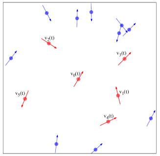
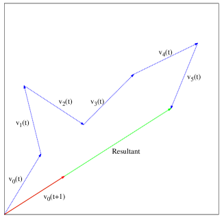
(a)	(b)

Figure 1: (Color online) (a) A flock of $N$ = 16 agents with $n=5$ neighbors in the interaction zone and at any arbitrary time $t$. The central agent is denoted by the subscript 0 and the velocity vectors of this agent and its 5 neighbors in the interaction zone are shown using red arrows. (b) In the next time step the velocity of agent 0 is calculated by Eqn. (1) which is along the resultant of all $n+1$ velocity vectors and has the magnitude $v$.

The generic feature of collective motion is, agents are short-sighted. While an individual agent’s behavior is influenced by the behavior of a small group of local agents around it, the whole group behaves in unison. In other words a short range interaction among the agents may lead to a unique global behavior of the entire group which implies the existence of a long range correlation among the agents. Therefore the question is, given a random distribution of positions and velocities what kind of short range dynamics can lead to global correlation reflected in cohesion and coherence among the agents.

This question was first explored in an assembly of self-propelled particles, known as the Vicsek model Vicsek . Here particles (agents) are released at random locations within a unit square box on the $x-y$ plane with periodic boundary condition and with random velocities. However, in the deterministic motion the direction of velocity of each agent $i$ is oriented along the resultant velocity ${\bf v}_{Ri}$ of all agents within an interaction zone (IZ) of range $R$ around $i$. In reality each agent may make an error in judging the resultant direction of motion and this has been introduced in the stochastic version of the model where noise is introduced by topping the orientational angle of ${\bf v}_{Ri}$ by a random amount $\Delta\theta$. Each individual agent is then moved along the updated velocity direction. A coherent phase is observed in the noise-free case with high agent densities. Moreover a continuous phase transition is observed on increasing the strength of noise where the mean flock speed continuously decreases to zero. However, facets like high density traveling bands occurring at low noise were revealed in later studies Chate1 ; Chate2 and arguments were put in favor of a discontinuous transition.

In a recent field study by the Starflag group on flocks of Starlings StarFlag , it has been shown that the interactions among the birds of a flock do not depend on the metric distance but on the topological distance. More quantitatively they found that each bird interacts with a fixed number of neighbors, about six or seven in number, rather than all neighbors within a fixed radial distance. Observing flocks of Starlings the angular density distribution of neighboring birds have been found to be anisotropic e.g., a bird is more likely to keep its nearest neighbor at its two sides rather than on the front and back. Fishes Gautrais have also been found to interact with neighbors determined by topological rules. Theoretical investigations Chate3 ; Chate4 revealed that the behavior of topology based models are very different from metric based models Heupe .

The concept of graph theory based topology was, however, used Jad to analyze the Vicsek model itself from the perspective of control theory. The metric distance based interactions were modeled using graphs with “switching topology”. Such studies also derived the conditions for the formation of coherent flocks for agents with fixed topologies Tanner1 . The relevance of underlying graphs or networks on the nature of collective motion has also been studied Bode1 ; Chate-nematics .

The observations of the StarFlag group prompted us to study the collective motion of flocking phenomena in two dimensions using the interactions depending on the topological distance. Most crucially we have obtained very interesting stationary states which have not been observed before, mainly the cyclic states. At the same time an increasingly large number of states are found to be completely cohesive and coherent. The paper is organized as follows. In section 2 we describe our topological distance dependent model for collective motion. The connectivity among such a collection of agents has been studied as the Random Geometric Graph in section 3. The stationary states of such flocks have been studied in section 4, the two most prominent states being the Single Sink State and the Cyclic State. The effect of the noise on the dynamics and the critical point of transition have been studied in section 5. Study of the dynamics of the flock with the fastest refreshing rate of the Interaction Zone has been done in section 6. A simpler version of the model with its vortex-antivortex states have been studied on the square lattice in section 7. Finally we summarize and discuss in section 8.

Figure 2: The undirected RGG with $N=1000$ nodes distributed randomly within a square box with a free boundary condition. Each node is linked to its $n$ nearest neighbors; $n$ = 1, 2, 3 and 4 increasing from left to the right. For small $n$ there are many components of the graph which merge with one another as $n$ increases. The largest component has sizes 9, 150, 988, 1000.

II 2. Model

In our model the interaction zone has been defined in the following way. During the flight, each agent $i$ interacts with a short list of $n$ other selected agents that constitute the IZ. It determines it’s own velocity using the Eqn. (1) given below following a synchronous dynamics. In general, the agent often refreshes the group of agents in IZ. For example, at the early stage, when the flock is relaxing to arrive at the stationary state and also during some stationary states, the inter-agent distances change with time. Every time the IZ is refreshed, we assume the criterion of selecting $n$ agents is that they are the first $n$ nearest neighbors of $i$. We introduce at this point a “refreshing rate” which controls how frequently an agent updates it’s IZ. In this paper we study two limiting situations when these rates are slowest and fastest. In the slowest rate, the agents do not change at all the the list of other $n$ agents in their IZs. The IZ for each agent, constructed at the initial stage, remains the same ever after, even if $n$ initial neighbors of an agent no longer remain nearest neighbors as time proceeds. The other limiting case is when the refreshing rate is the fastest, the IZ is refreshed for every agent at each time step. The slowest case has been discussed in sections 4 and 5. The fastest refreshing rates have been discussed in section 6. For the spins on the square lattice discussed in section 7, these two cases actually mean the same since the spins are firmly fixed at their lattice positions.

The number $n$ of agents in IZ is considered as an integer parameter of the model. As in Vicsek model Vicsek the system is updated using a discrete time dynamics. While the speeds $v$ of all agents are always maintained to be the same, the orientational angles $\theta_{i}$ of their velocities are updated by the direction of the resultant of velocity vectors of all $n$ agents in the interaction zone and the agent $i$ itself (Fig. 1),

$$\theta_{i}(t+1)=\tan^{-1}[\Sigma_{j}\sin\theta_{j}(t)/\Sigma_{j}\cos\theta_{j}(t)]$$ (1)

where the summation index $j$ runs over all $(n+1)$ agents in IZ. The whole flock moves in the infinite space. Following this dynamics, the flock reaches the stationary state after a certain period of relaxation time. It is observed that the stationary state depends on the initial positions, initial velocities of the agents, as well as the neighbor number $n$. Though a number of different stationary states have been observed, often the state is a fixed point or a cycle. We have studied the statistical properties of these fixed points and cycles and observed that cohesion and / or coherence are indeed present in different stationary states.

There are two crucial differences of our model and the Vicsek’s model which we summarize as follows: a) We have used the same prescription of interaction that had been claimed in the StarFlag experiment. Accordingly, an agent here interacts with a fixed number $n$ of nearest neighbors and not on all neighbors up to a fixed radial distance. It may be noted that, these two mechanisms are essentially serving the same purpose. Both prescriptions keep the mutual interactions active among the local agents only. Therefore our choice of neighbourhood and Vicsek model’s range of interaction are actually on the same footing.(b) No periodic boundary condition is imposed in our model. Therefore agents move out in open space, yet they often form flocks that exhibit considerable amount of cohesion and coherence. Compared to the Vicsek model, use of the free boundary condition makes our model less restrictive.

In the limiting case, when the IZ is refreshed at the slowest rate, it may appear that for an agent, any of the $n$ neighbours can be at an arbitrarily large distance. Certainly this is not the case for a cohesive and coherent flock by definition. Moreover, we will see in the following that for most of the stationary states, the neighboring agents indeed remain within the close proximity of an agent.

III 3. Random Geometric Graphs

At the initial stage $N$ agents are uniformly distributed at random locations within a unit square box on the $x-y$ plane without periodic boundary condition. A random geometric graph (RGG) RGG is constructed whose vertices are the agents. At the same time for any arbitrary pair of vertices $i$ and $j$, $j$ is defined as a neighbor of $i$ if it is among the $n$ vertices nearest to $i$. Then an edge is assumed to exist from $i$ to $j$. This implies that the edges are in general ‘directed’ since if $j$ is the neighbor of $i$ then $i$ may or may not be the neighbor of $j$. Therefore the resulting graph is inherently a directed graph. However one can also define a simplified version of the graph by ignoring the edge directions and consider the graph as an undirected graph. In the following we refer such an undirected graph as the RGG.

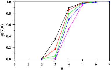
Figure 3: (Color online) The fractions $g(N,n)$ of single component connected graphs, in a sample of 1000 RGGs, are plotted against $n$. For $N$ agents this fraction grows as the number of neighbors $n$ is gradually increased. System sizes $N$ are 256 (black), 512 (red), 1024 (green), 2048 (blue) and 4096 (magenta), increased from left to right. The number of independent configurations used for each value of $n$ is 1000.

In Fig. 2 we exhibit the pictorial representation of an undirected RGG for $N=1000$ as $n$ is increased step by step. For small values of $n$ the graph has many different components. As $n$ is increased the components grow gradually in size, merge into one another and finally the RGG becomes a single component connected graph covering all vertices for a certain value of $n$. Here we have shown four figures for $n$ =1, 2, 3 and 4. The randomly selected positions of all vertices are exactly the same in these figures. The size of a component is measured by the number of vertices in that component. In this figure the RGG becomes fully connected for $n$ = 4.

The structure and connectivity of RGG depend on the initial positions of $N$ vertices. Therefore we have first studied how the fraction $g(N,n)$ of connected graphs grows with $n$ when the flock size $N$ is increased. For a particular RGG the connectivity is checked using the ‘Burning Algorithm’ Herrmann where the fire, initiated at an arbitrary vertex, propagates along the edges and finally burns all vertices if and only if the RGG is a single component connected graph.

In Fig. 3 we show the plots of $g(N,n)$ against $n$ for different values of $N$. To find out if a minimum value of the neighbor number $n$ exists, one can artificially prepare a linear initial configuration of agents where each agent has it’s right neighbor as the nearest one. This corresponds to $n=1$ but occurrence of such a configuration by random selection of positions of the agents is extremely improbable. Numerically we find that for small $n$ the $g(N,n)$ takes vanishingly small values. However, on increasing $n$, $g(N,n)$ increases very rapidly and when $n$ is around 7, $g(N,n)\approx 1$ i.e., nearly all configurations become connected. With increasing flock size $N$ the curves slowly shifts to higher values of the neighbor number $n$.

Only those flocks whose RGGs are single component connected graphs are considered for their dynamical evolution. The initial neighbor list is maintained for the entire dynamical evolution of the flock and is never updated even if all $n$ initial neighbors of an agent no longer remain nearest neighbors as time evolves. This means that the set of agents’ velocities $\{\vec{v}_{i}(t+1)\}$ is fully determined using the detailed knowledge of the set $\{\vec{v}_{i}(t)\}$. Implication of this is, the positions and velocities are completely decoupled during the time evolution since the actual positions of agents do not play any role to determine the velocities. Therefore the topological connectivity of RGG remains invariant and is a constant of motion.

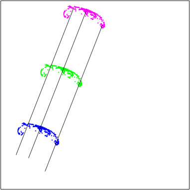
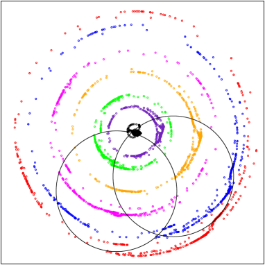
(a)	(b)

Figure 4: (Color online) Flocks of size $N$ = 512 and $n=10$, moving with the speed of $v$ =0.03 without noise. (a) Single sink state: The fully cohesive and coherent motion of the flock is exhibited by its position at three different instants: 10000 (blue), 11000 (green) and 12000 (magenta). Three straight line trajectories of individual agents are also shown. The frame size is $90\times 90$ units. (b) Cyclic state: The stationary state pulsating flock has been shown at different time instants: 173,000 (black), 176000 (red), 180000 (green), 188000 (blue), 192000 (brown), 197000 (violet) and 200000 (magenta). The time period is 28835. Two individual agents’ circular trajectories with radius $\approx 137.67$ are also shown. The frame size is $600\times 600$ units.

IV 4. Stationary States

IV.1 4.1. Single Sink States

Initially the $N$ agents are randomly distributed with uniform probabilities within the unit square box on the $x-y$ plane. If the corresponding RGG is fully connected then all agents are assigned the same speed $v$ but along different directions. The angles $\theta_{i}$ of the velocity vectors with respect to +$x$ axis are assigned by drawing them randomly from a uniform probability distribution between 0 and $2\pi$. As time proceeds the agents soon come out of the initial unit square box and spread out in the open two dimensional space. After some initial relaxation time the flock arrives at the stationary state. One of the most common stationary state is the one where the flock is completely coherent and cohesive. The entire flock moves along the same direction without changing the flock’s spatial cohesive shape and therefore $\theta_{i}(t)={\it C}$ for all $i$ and are independent of time. We call these states as the ‘Single Sink States’ (SSS). Therefore this stationary state is a fixed point of the dynamical process. A picture of such a flock has been shown in Fig. 4(a).

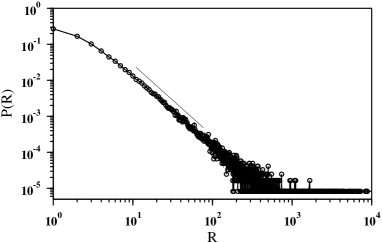
Figure 5: The probability distribution of the radii of the individual agent’s circular orbits in the cyclic states. The power law has an exponent of $\tau=1.99(2)$.

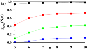
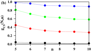
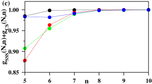
Figure 6: (Color online) The occurrence of two most prominent stationary states when the neighbor number $n$ has been varied over a range from 5 to 10 and for for different flock sizes $N$ = 64 (black), 256 (red), 512 (green) and 1024 (blue). (a) The fraction $g_{SSS}(N,n)$ of SSS has been plotted against $n$. (b) The fraction $g_{CS}(N,n)$ of CS has been plotted against $n$. (c) The sum of $g_{SSS}(N,n)+g_{CS}(N,n)$ has been plotted and it is seen that beyond $n\approx 8$ the sum is approximately unity.

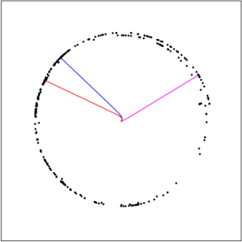
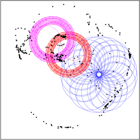
(a)	(b)	(c)

Figure 7: (Color online) Flocks of size $N$ = 512 and $n=5$, moving with the speed of $v$ =0.03 without noise. The positions of the agents are marked by black dots and three individual agent’s trajectories are shown in each case by red, blue and magenta colors. (a) Distributed sink state: Every agent moves along a fixed direction $\theta_{i}={\it C}_{i}$ of its own which is different in general from the directions of motion of other agents. (b) Cycloid state: In the stationary state the trajectory of each agent is a cycloid. (c) Space-filling state: The trajectory of an agent never repeats itself but gradually fills up the space between two concentric circles. The frame sizes are 40000, 15000 and 350 units respectively.

IV.2 4.2. Cyclic States

In cyclic states the velocity directions $\theta_{i}$ of all agents change at a constant rate in absence of noise. Therefore the angular velocity $\dot{\theta}_{i}(t)={\it D}$ for all agents is a constant of motion. Each agent moves in a circular orbit of its own depending on its initial position, but their radii and time periods are the same. Consequently the magnitude of the resultant velocity of the whole flock in the CS has also a constant value but its direction changes with the same angular velocity. In addition typically the shape of the flock is another circle though with some irregularities and interestingly its radius changes periodically with the same period of individual agents. Therefore the whole circular flock pulsates, i.e., periodically expands and contracts where each agent moves on its own fixed circular trajectory. We explain this motion in Fig. 4(b) by plotting the flock at different instants of time and also show two individual agent trajectories. We call these states as the ‘Cyclic States’ (CS).

For an arbitrary CS, let the probability that the radius of individual agent’s circular trajectory between $R$ and $R+dR$ be $P(R)dR$. Given that the uniform speed of the agents is $v$ and their angular velocities is $\dot{\theta}$, the radius of the circular trajectory is $R=v/\dot{\theta}$. We have studied a large number of such cyclic states and measured the radii of the agents’ orbits. In Fig. 5 we show the probability distribution of these radii which follows a power law distribution $P(R)\sim R^{-\tau}$ with $\tau=1.99(2)$.

Throughout this paper we have used only one value of the agent speed, i.e., $v$ = 0.03. If the speed is reduced by a certain factor a CS state remains CS but all the characteristic lengths are reduced by the same factor. The radius of the circular orbit of every agent and also the size of the flock are reduced by the same factor, the time period remaining the same. Therefore it appears that even in the continuous limit of $v\to 0$, the characteristic features of the flocks reported here remain same.

Starting from the initial state, when the random positions and velocities are assigned to all agents, the fractions of stationary states that exhibit the SSS and CS are estimated and are denoted by $g_{SSS}(N,n)$ and $g_{CS}(N,n)$ respectively. In Fig. 6 these two quantities are plotted against the neighbor number $n$ for different flock sizes $N$. For a certain $N$, $g_{SSS}(N,n)$ gradually increases with increasing $n$ (Fig. 6(a)). For a given flock size $N$, however large, if the neighbor number $n$ is increased to $N-1$, then on using the dynamics mentioned in Eqn. (1) the stationary state flock must be both cohesive and perfectly coherent i.e., $g_{SSS}(N,N-1)=1$. No stationary state other than SSS can exist in this limiting situation. On the other hand when $n<N-1$ but $n$ is increased, then $g_{SSS}(N,n)$ also gradually increases and approaches the value of unity for any arbitrary value of $N$. At the same time, $g_{CS}(N,n)$ decreases with $n$ for a fixed $N$ but increases with $N$ for a fixed $n$ (Fig. 6(b)). Finally in Fig. 6(c) we plot the sum $g_{SSS}(N,n)+g_{CS}(N,n)$ which is less than unity for small $n$, but on increasing $n$, this sum gradually increases and reached $\approx 1$ for $n=8$ for all $N$. It is therefore concluded that if the neighbor number is increased all other states gradually disappear and only SSS and CS states mostly dominate but ultimately for even larger value of $n$ it is the SSS state that only survives.

IV.3 4.3. Other states

In addition there are a number of other stationary states, few of them are described below, but the list may not be exhaustive.

(i) Each agent has a constant velocity but their directions are different for different agents. For example the $i$-th agent has its direction of velocity $\theta_{i}={\it C}_{i}$. In this case the agents, after some relaxation time, moves outward radially. The shape of the flock is approximately circular, again with some irregularities, and the radius of the flock increases at a uniform rate. We call these states as the ‘Distributed Sink States’(DSS). In Fig. 7(a) an example of the DSS has been shown. The position of the flock is shown at $t=$ 500000 and three agents’ trajectories have been shown using different colors.

(ii) In another type of stationary state the trajectories of the individual agents are very similar to cycloids. Each agent moves radially outward in a nearly cycloidal motion (Fig. 7(b)). A considerable number of agents form a flock of circular shape but others are scattered around this circular flock. We call these as ‘Cycloid States’.

(iii) Thirdly there can be rosette type stationary states. The trajectory of each agent is like a rosette which never closes and lies between two concentric circles. Consequently in the long time limit the trajectories fill the space between the two circles. This means that the mean separation between consecutive intersections of the agent trajectory with a radial section gradually vanishes as the trajectory evolves for a longer time. We call these as ‘Space-Filling States’. Three such rosette trajectories and the position of the flock have been shown in Fig. 7(c).

Few points may be mentioned here about the characteristics of the different stationary states. For example a possible anisotropic effect on the stationary states may exist due to the choice of the unit square box for releasing the agents. Initially the positions of the agents are selected randomly within unit square box on the two dimensional plane. We have compared that if the agents’ locations are selected randomly within a circle of radius 1/2, no appreciable change have been observed in the fractions of different stationary states.

The center of mass of the entire flock has different kinds of trajectories in different stationary states. In SSS, the center of mass moves in a straight line exactly similar to all other agents. In CS, the trajectory of the center of mass is also a circle, but it’s radius is not the same as the radius of the orbit of the individual agents, but it is some what larger. In DSS the dynamics of the center of mass is similar to that of the agents. Although, the shape of the flock is approximately circular, but the fact that, at any instant the positioning of the agents on the circumference is not uniform, makes the center of mass move radially outwards in a straight line. Motion is indeed unbounded. In cycloid states, the trajectory of the center of mass is also a cycloid and radially outwards. The motion here is also unbounded. In space filling states, the trajectory of the center of mass is rosette type. In this case the trajectory is bounded.

How sensitive are the final stationary states on the choice of the random initial values of $\{x_{i},y_{i}\}$ and $\{\theta_{i}\}$ for the $N$ agents? To study this point, we tried with a flock that evolves from a certain initial configuration that evolves to a CS. Now we again evolve the same flock, but this time we slightly change the initial configuration randomly by $x_{i}=x_{i}+a.10^{-4}.r$ and $y_{i}=y_{i}+a.10^{-4}.r$ where $r$ is a random number. The directions $\{\theta_{i}\}$ of the velocity vectors are maintained the same. We then tune $a$, and found that with $0<a<1.70$ the stationary state is still a CS, but with different values of the orbit radius. When $a\geq 1.75$ the stationary state becomes SSS. We conclude that with some amount of perturbation the character of the stationary state remains same, but with even stronger perturbation the stationary state changes.

A preliminary calculation with our model in three dimensions shows the following features. In general, to obtain connected graphs, the value of $n$ needs to be large compared to what is required in two dimensions. Almost always the dynamics leads to a SSS in the steady state. We did not find any other state starting from random initial conditions.

V 5. Dynamics in presence of noise

Studying the role of noise on the dynamics of the flock is very crucial. It is assumed that every agent makes a certain amount of error in judging the angle of its velocity vector at each time step. More precisely given the angles $\theta(t)$ of velocity vectors of all $n+1$ agents within the interaction zone at time $t$, it first calculates the resultant of these vectors using the Eqn. (1). It then tops up this angle by a random amount $\zeta(\eta)$ which is uniformly distributed within $\{-\eta/2,\eta/2\}$. Therefore the modified Eqn. (1) reads as:

$$\theta_{i}(t+1)=\tan^{-1}[\Sigma_{j}\sin\theta_{j}(t)/\Sigma_{j}\cos\theta_{j}(t)]+\zeta(\eta).$$ (2)

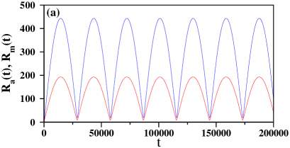
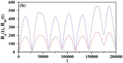
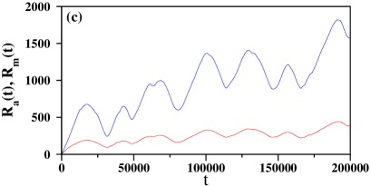
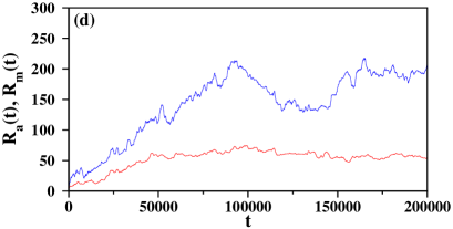
Figure 9: (Color online) Effect of noise is exhibited on a single flock ($N$ = 512 agents, each having $n$ = 10 neighbors) which goes to a cyclic state without any noise. Variation of the maximal radius $R_{m}$ (blue) and the average radius $R_{a}$ (red) have been shown with different strengths of the noise parameter: (a) $\eta=0$, (b) 0.2, (c) 0.5 and (d) 1. The initial positions and velocities are same in all four cases.

The role of the noise is to randomize the deterministic dynamics and quite expectedly the stationary state structures of the flocks exhibited in the SSS and CS patterns are gradually lost. We have studied the effect of noise on both these states by gradually increasing the strength of the noise $\eta$. In both cases we use a flock of $N$ = 512 agents, each of them interacts with $n=10$ nearest neighbors and travel with speed $v=0.03$. Initially all of them are released within the square box of size unity. We first run the dynamics without any noise i.e., $\eta=0$ and ensure that the stationary state pattern is indeed a single sink state. As the dynamics proceeds we calculate the maximal distance $R_{m}(t)$ and the average distance $R_{a}(t)$ of an agent from the center of mass $(x_{c}(t),y_{c}(t))$ of the flock. In Fig. 8(a) we plot these two quantities against time and they are exactly horizontal curves which are the signatures of the SSS state. These simulations are then repeated for $\eta>0$ and the variations of $R_{m}(t)$ and $R_{a}(t)$ have been shown in Figs. 8(b), 8(c) and 8(d) for $\eta=0.2,0.5$ and 1 respectively. In all four cases the flock starts with the same positions and velocities of the agents. It is seen that on increasing the strength of noise the stochasticity gradually sets in and the variations of $R_{m}(t)$ and $R_{a}(t)$ gradually become random. A similar plot has been exhibited in Fig. 9 for the CS but for only a single flock. The Fig. 9(a) shows the zero noise case and the curves are periodic. However when the noise level is increased (Figs. 9(b)-(c)) it distorts the periodicity. With small values of $\eta$ the variations are slightly distorted from the periodic variations, however with larger strength of noise the distortion is much more. Finally for $\eta=1$ the fluctuations look random and similar to those in the SSS (Fig. 9(d)).

Next we calculated the mean square displacement $\langle r^{2}(t,\eta)\rangle$ from the origin as time passes. The averaging has been done for a single agent within a flock and over many such independent flock samples. The noise strength has been varied over a wide range of values. In Fig. 10 we have displayed the variation of $\langle r^{2}(t,\eta)\rangle$ against the time $t$ using a $\log-\log$ scale for six different values of $\eta$. Here again we consider flocks with fully connected RGGs. On the other hand with zero noise these configurations may lead to any of the possible stationary states. Simulating up to a maximal time of $T=10^{8}$ we observed a cross-over behavior in the mean square displacement. When $\eta$ is very small $\langle r^{2}(t,\eta)\rangle\sim t^{2\kappa}$ with $\kappa\approx 1$ which implies that the flock maintains a ballistic motion at the early stage, i.e., the coherence is still maintained during this period. On the other hand after a long time one gets $\kappa=1/2$ which indicates the diffusive behavior. This implies that even if a little noise is applied for a long time, the effect of the noise becomes so strong that the flock can no longer maintain a cohesive and coherent structure any more and agents diffuse away in space. Therefore for any value of $\eta$ there is a cross-over from the ballistic to diffusive behavior. Consequently a cross-over time $t_{c}(\eta)$ can be defined such that for short times $t<<t_{c}(\eta)$ the dynamics is ballistic with $\kappa=1$ and for $t>>t_{c}(\eta)$ the dynamics is diffusive with $\kappa=1/2$. In Fig. 10 we show this behavior and observe that the crossover time depends explicitly on the value of $\eta$ and diverges as $\eta\to 0$. The value of $t_{c}(\eta)$ has been estimated by the time coordinate of the point of intersection of fitted straight lines in the two regimes of Fig. 10: for $t<<t_{c}(\eta)$ and for $t>>t_{c}(\eta)$. The value of $t_{c}(\eta)$ so estimated diverges as $t_{c}(\eta)\sim\eta^{-2.52}$.

This transition is more explicitly demonstrated using a plot of the Order Parameter (OP) $M(\eta)$ against $\eta$ (Fig. 11). The OP is defined as the time averaged magnitude of the resultant of all agents’ velocity vectors, scaled by its maximum value

$$M(\eta)=\langle|\Sigma^{N}_{j=1}{\bf v}_{j}|\rangle/(Nv)$$ (3)

where $\langle...\rangle$ denotes the time average over a long period of time in the stationary state. In Fig. 11 (a) we have plotted $M(\eta)$ against $\eta$ at an interval of $\Delta\eta=0.1$ for different system sizes from $N$ = 64 to 1024. In these simulations the initial conditions are chosen to be completely coherent so that the velocity vectors of all agents are in the same direction. In the absence of noise this situation is maintained and $M(0)=1$ at all times for all system sizes. However for $\eta>0$ noise sets in, but in the stationary state one still gets a non-zero OP. On further increasing $\eta$ the OP decreases monotonically and ultimately vanishes. Therefore there exists a critical value $\eta_{c}(N)$ of the noise parameter where the transition from the ordered state to disordered state takes place. It is observed in Fig. 11(a) that as the system size $N$ is enlarged the transition becomes more and more sharp and shifts to the regime of small $\eta$. Further we have calculated the Binder cumulant $G(\eta)=1-\langle M^{4}(\eta)\rangle/3\langle M^{2}(\eta)\rangle^{2}$ and plotted against $\eta$ in Fig. 11(b) for the same system sizes Binder . The value of $G(\eta)$ drops from a constant value of around 2/3 at the small $\eta$ regime to about $1/3$ for large values of $\eta$.

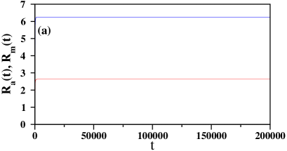
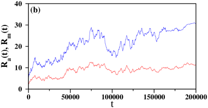
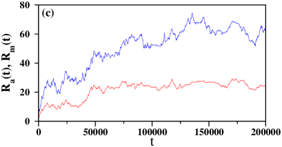
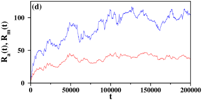
Figure 8: (Color online) Effect of noise is exhibited on a single flock ($N$ = 512 agents, each having $n$ = 10 neighbors) which goes to a single sink state without any noise. Variation of the maximal radius $R_{m}$ (blue) and the average radius $R_{a}$ (red) have been shown with different strengths of the noise parameter: (a) $\eta=0$, (b) 0.2, (c) 0.5 and (d) 1. The initial positions and velocities are same in all four cases.

The transition point $\eta_{c}$ can be estimated in the following two ways. For each curve in Fig. 11(a) we calculate the value of $\eta_{1/2}(N)$ for which $M(\eta)=1/2$. We define $\eta_{1/2}(N)$ is the characteristic noise level where the transition takes place. By interpolation of the plots in Fig. 11(a) of the points around $M(\eta)=1/2$ we have estimated $\eta_{1/2}(N)$. These estimates are then extrapolated in Fig. 11(c) as:

$$\eta_{1/2}(N)=\eta_{1/2}(\infty)+AN^{-1/\nu}.$$ (4)

On tuning the trial values of $\nu$ very slowly we found that for $\nu\approx 2.86$ the error in the least square fit of the above finite-size correction formula is minimum. Therefore the extrapolated $\eta_{1/2}(\infty)\approx 1.70$ is the critical noise strength $\eta_{c}$ according to our estimate. A similar calculation has also been done using the Binder cumulant. From this calculation we estimated $\eta_{c}=1.82$ and $\nu=3.50$. The differences between the two estimates are considered as the error in the measured values which are 0.12 and 0.64 for $\eta_{c}$ and $\nu$ respectively.

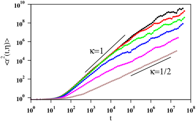
Figure 10: (Color online) The mean square displacement $\langle r^{2}(t,\eta)\rangle$ of an agent from the origin has been plotted against time for different values of the noise parameter $\eta$ = 0.2 (black), 0.5 (red), 1.0 (green), 2.0 (blue), 3.0 (magenta) and 4.0 (brown). The flock size $N=512$ and the neighbor number $n=10$. Two short straight lines are the guides to the eye whose slopes are $\kappa=1/2$ and 1.

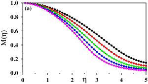
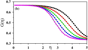
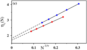
Figure 11: (Color online) (a) The stationary state order parameter $M(\eta)$ and (b) the Binder cumulant $G(\eta)$ have been plotted for the system sizes $N$ = 64 (black), 128 (red), 256 (green), 512 (blue) and 1024 (magenta) where all agents start with their initial velocities in the same direction. System size increases from right to left. (c) Extrapolation of $\eta_{c}(N)$ values determined from (a) and (b). We obtained $\eta_{c}(N)=1.70+N^{-1/2.86}$ and $\eta_{c}(N)=1.82+N^{-1/3.50}$ respectively.

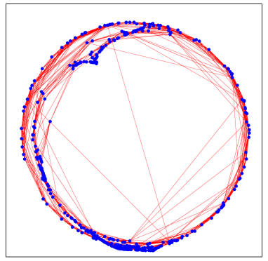
Figure 12: (Color online) The position of a flock ($N$ = 512, $n$ = 10) in CS by blue dots and links by red lines. The frame size is 150 units.

Since the agents are uniformly distributed initially, the edges of RGG also are homogeneously distributed as shown in Fig. 2(d). However with time evolution these edges change their positions but their connectivity do not change, i.e., the end nodes of every edge are always fixed since the neighbor list does not change. How they look in the stationary state has been exhibited in Fig. 12. This is the picture of the circle shaped flock in the cyclic state. The blue dots represent the agents and the red lines represent the edges. What is interesting to note is that the system self-organizes itself so that not only agents but also the edges are constrained to be within a very limited region of the space. Very few edges criss-cross the flock from one side to the opposite side. Initially each agents had its $n$ neighbors at its closest distances. After passing through the relaxation stage and arriving at the stationary state, when the shape of the flock is completely different from its initial shape, most of the agents maintain their connections with other agents in their local neighborhood only.

VI 6. The fastest refreshing rate of the Interaction Zone

Here we consider the case corresponding to the fastest refreshing rate of the interaction zone, i.e., when every agent updates its $n$ nearest neighbors at every time step. Consequently, the RGG is no longer a constant of motion in this case and is updated at each time step. While performing simulations of this version, we first notice that in the long time stationary state the entire flock becomes fragmented with probability one into different clusters. For a flock of $N$ agents with neighbor number $n$, the minimum number of agents in a cluster is $n+1$. An agent of a particular cluster has all $n$ neighbors which are members of that cluster only. In the stationary state all agents of a cluster has exactly the same direction of velocity and the entire cluster moves along this direction with uniform speed $v$. Therefore, the velocity direction $\theta$ of a particular cluster can be looked upon as the identification label of that cluster. The shape of the flock is approximately circular since each cluster travels outward with same speed (Fig. 13(a)). Moreover, within a cluster if the agent $i$ is a neighbor of the agent $j$ then $j$ is also a neighbor of $i$. Therefore the sub-graph of the entire RGG specific to a cluster is completely undirected and the corresponding part of the adjacency matrix is symmetric (Fig. 13(b)). This immediately implies that the $N\times N$ adjacency matrix of the entire flock can be written in a block-diagonal form by assigning suitable identification labels of different agents.

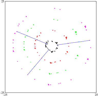
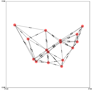
(a)	(b)

Figure 13: (Color online) (a) Positions of a flock of $N$ = 512 agents with $n=5$ neighbors in the interaction zone and at four different time instants: 100 (black), 200 (red), 300 (green) and 400 (magenta). The RGG has been updated at every time step. Three individual agents’ straight line trajectories have also been shown. There are a total of 29 clusters. (b) The sub-graph of the RGG corresponding to a specific cluster of 16 agents have been shown. An arrow has been drawn from the agent $i$ to the agent $j$ if $j$ is one of the $n$ neighbors of $i$. There are a total of $16\times 5$ = 80 distinct links and each link is directed in both directions. It may also be noted that whole set of links are restricted to the nodes of the cluster only.

A natural question would be how the probability distribution $D(s)$ of different cluster sizes depends on the cluster size $s$. To answer this question a large number of independent flocks have been simulated and each of them was evolved to its stationary state. In the stationary state the sizes of the individual clusters are measured using the burning method. In Fig. 14(a) a plot of $D(s)$ vs. $s$ for $s>n$ has been shown on a semi-log scale for $N$ = 512 and $n$ = 5, the data being collected using a sample size of 20000 independent flocks. Apart from some noise at the tail end and a maximum around the smallest value of $s$ the plot fits well to a straight line, implying an exponentially decaying form of the probability distribution. We conclude $D(s)\sim\exp(-s/s_{c})$ where $s_{c}\approx 7.2(1)$.

Next, the average number of clusters $\langle n_{s}(N,n)\rangle$ has been calculated and plotted in the inset of Fig. 14(b) for $N$ = 128, 256 and 512 and $n$ = 5 on a $\log-\log$ scale. Again, apart from the tail end, the plots fit very nicely to parallel straight lines, the slopes of which are estimated to be 1.168(5). In the main part of Fig. 14(b) a scaling has been shown which exhibits a nice data collapse, corresponding to the following form

$$\langle n_{s}(N,n)\rangle N^{-1.1}\sim n^{-1.168}.$$ (5)

This implies that as the neighbor number $n$ increases, there would be fewer clusters in the stationary state. On the other hand, for a specific value of $n$, the average cluster number grows with the flock size as $N^{1.1}$. Assuming that the above scaling relation holds good for the entire range of $n$, for a given $N$ one can define a cut-off value of $n=n_{c}$ such that $\langle n_{s}(N,n_{c})\rangle$ = 1 which leads to $n_{c}(N)\sim N^{1.1/1.168}=N^{0.94}$. However our simulations suggest that due to the presence of an upward bending at the tail end, the above scaling relation does not work at this end and $n_{c}(N)$ is actually of the order of $N$.

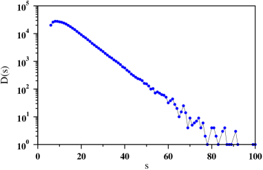
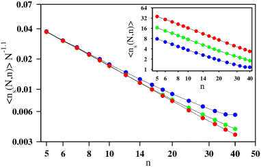
(a)	(b)

Figure 14: (Color online) (a) The probability distribution $D(s)$ of the cluster sizes $s$ seems likely to have an exponentially decaying form $\exp(-s/s_{c})$ where $s_{c}\approx 7.2$. (b) The inset shows the plot of the average cluster size $\langle s(N,n)\rangle$ for $N=512$ and $n=5$ with neighbor number $n$ on a $\log-\log$ scale: $N$ = 128 (blue), 256 (green) and 512 (red). In the main plot the vertical axis has been scaled by $N^{1.1}$ which leads to a data collapse.

VII 7. Vortices on the square lattice

In this section we studied a simpler version of our model where every agent is a spin vector. They are no more mobile, their positions are completely quenched at the sites of a regular lattice, but the directions $\theta_{i}(t)$ of the spins are the only dynamical variables that evolve with time following Eqn. (1). More specifically, spins are placed on a square lattice with different choices for the first $n$ neighbors and we study the spatio-temporal patterns that emerge during the time evolution of the angular variables $\{\theta_{i}(t)\}$. The arrangement of the spins allows to draw a parallel with the dynamics of planar spins in the two dimensional $XY$ model.

The connections between the Vicsek model Vicsek and the $2d$ $XY$ model KT have been explored since long toner-tu ; Chate-nematics ; toner-tu-ram . It is well known that in the limit of speed $v\to 0$ the dynamics of the Vicsek model would exactly map on to the finite temperature Monte Carlo dynamics of the $2d$ $XY$ model. However, in the latter model any long-range ordered phase is absent. Instead a quasi-long-range ordered phase appears at the low temperatures and the transition to the disordered phase is associated with the simultaneous unbinding and increase of vortex-antivortex (VAV) pairs. In the low temperature phase VAV pairs are to be found in tightly bound states. We find that our model defined on the square lattice also gives rise to VAV pairs and we determine the density of such pairs, as a function of the noise amplitude $\eta$.

We define the IZ of an agent with respect to its $n$ nearest neighbors on the square lattice of size $L\times L$ with the periodic boundary condition. For $n=2$, the IZ includes the top and the right nearest neighbors. For $n=3$, the left nearest neighbor is also included and in the case of $n=4$, all the four nearest neighbors are included. We notice that for the $n=4$ case, the Vicsek model with spins similarly placed on the square lattice and interact with a range $R=1$ and our model are same. As before we study the dynamics of the spin system with and without noise.

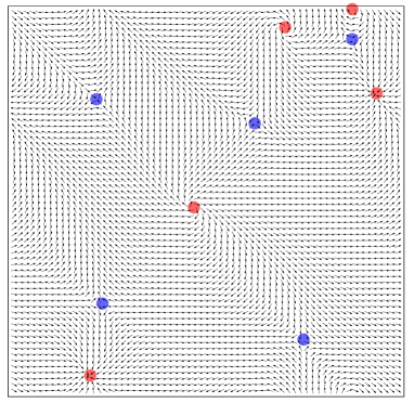
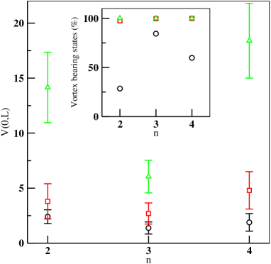
(a)	(b)

Figure 15: (Color online) (a) Vortex-antivortex pairs of the spin systems in the stationary state in a square lattice with size $L=64$ and $n=2$ with zero noise. The orientations of the spins change with time in such a way so that the entire spin pattern with vortices and the antivortices move with a uniform speed from the top-right corner to the bottom-left corner. Vortices and antivortices are marked by filled red and blue circles. (b) The number $V(0,L)$ of vortex-antivortex pairs at zero noise for different values of $n$ in lattices of three different sizes: $L=32$ (circles), $64$ (squares) and $128$ (triangles). The bars indicate the standard deviation in the values obtained from around $100$ configurations in each case. In the inset the percentage of configurations which lead to steady states with vortex pairs is plotted against $n$.

In the absence of noise, beginning from arbitrary initial conditions for $\theta_{i}$’s, the dynamics results in the formation of VAV pairs. For $n=2$ and 3, the interactions are anisotropic. Consequently the entire spin pattern in the stationary state as well as all VAV pairs are mobile and in general all the spin orientations $\theta_{i}$’s change with time. In comparison, for $n=4$, all the $\theta_{i}$’s remain frozen in time which also implies that all the VAV pairs are anchored. We find that the choice of the IZ, in addition to the periodic boundary condition, fixes the direction of motion of the VAV pairs. In the Fig. 15(a) an instantaneous configuration of the spins is plotted for a lattice with $L=64$ and $n=2$. In general for the $n=2$ case the entire spin pattern moves on the average along the diagonal direction from top-right to bottom-left. For the case, $n=3$, the vortices travel from the bottom to the top.

Let the $V(\eta,L)$ be the number of VAV pairs observed at noise $\eta$ in lattice of size $L$. The number of VAV pairs observed at zero noise, $V(0,L)$ is plotted against the value of $n$ in the Fig. 15(b) for different lattice sizes. We observe during the time evolution for a given initial condition that the number of VAV pairs initially decays and then becomes stationary. However, different initial conditions leads to different values at the stationary states. The bars indicate the dispersion that is observed for different initial conditions which lead to non-zero number of VAV pairs. For the lattice size $L=128$ we wait for $10^{5}$ steps before calculating number of VAV pairs. The inset to the Fig. 15(b) shows the percentage of initial conditions that lead to non-zero number of VAV pairs. We find as lattice size increases, arbitrary initial conditions, almost always, lead to states with VAV pairs.

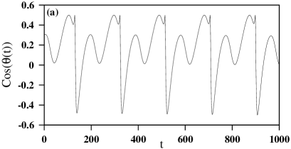
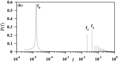
Figure 16: (Color online) (a) The $x$-component of a typical spin vector is plotted against time for lattice with $L=64$ and $n=2$ at zero noise. (b) The corresponding power spectrum indicates the presence of three basic frequencies $f_{0}=1/(4096L)$, $f_{1}=1/(3L)$ and $f_{2}=2/(3L)$. The higher frequencies can be expressed as combinations of the $f_{1}$ and $f_{2}$ and essentially become harmonics of $f_{1}$ since $f_{2}=2f_{1}$.

The nature of the time variation of the spin angle $\theta_{i}$’s for the cases $n=2$ and $n=3$ are found to be quite complex. In the Fig. 16(a) we plot the time series corresponding to the oscillation of the $x$-component of a typical spin vector for $L=64$ and $n=2$. The corresponding power spectrum apparently reveals the presence of three basic frequencies $f_{0}$, $f_{1}$ and $f_{2}$ all of which are rational multiples of $1/L$ (Fig. 16(b)). The time evolution can be explained as a periodic oscillation with $f_{1}$ and $f_{2}$ (since $f_{2}=2f_{1}$) riding on a very slow mode. These features carry over to $L=128$ as well. We find that in the case of $n=3$, the spectrum is similar but the frequencies are not simple multiples of $1/L$.

It is known that metastable vortices are produced at low temperatures in the $2d$ $XY$ model when equilibrium is achieved beginning from arbitrary initial conditions. However, these vortices are not responsible for the VAV unbinding transition miyashita . Therefore, we study the effect of noise by “cooling down” tobochnik the system to zero noise level starting from a high value of noise. At each noise level the system initially passes through $10^{5}$ time steps; after this relaxation it passes through an additional $10^{4}$ time steps and then moves to the next lower level of noise. We begin around the value of noise given by $\eta=3.7$ and decrease $\eta$ by an amount $0.07$ in each step. This method suppresses the generation of the VAV pairs at low noise. At zero noise the vortices are absent in contrast to the statistics discussed in the previous paragraphs where the cooling down method was not employed.

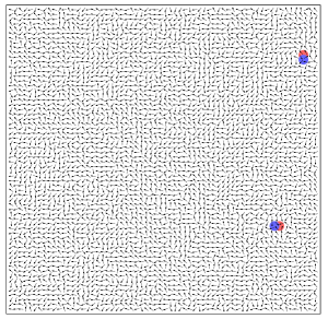
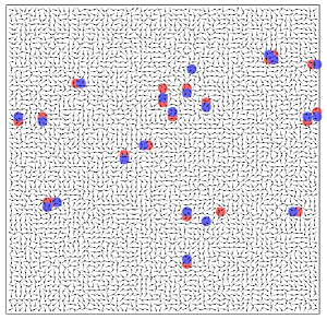
(a)	(b)	(c)

Figure 17: (Color online) The figure shows proliferation of vortices as noise is increased in a square lattice of length $L=64$ with $n=4$. (a) For $\eta=0.15$ there are no vortices, (b) for $\eta=0.35$ vortices begin to appear, there are only two vortex-antivortex pairs and (c) for $\eta=0.40$ twenty one vortex-antivortex pairs can be seen. Filled circles of two different colors, red for vortices and blue for antivortices, have been drawn around the vortex centers.

At zero noise we find the spin system reaches the globally ordered state where all the spin vectors are oriented in the same direction. We believe that this is due to the finite size effect of the lattice. The spin configuration at low noise of $\eta=0.15$ has been shown in the Fig. 17(a) for $L=64$ and $n=4$ where not only vortices are absent but the long-range order is also not present. At the higher noise levels VAV pairs start appearing and there is a rapid increase in the number of pairs with further increase in noise. All the VAV pairs appearing initially are tightly bound i.e., lattice spacing is small between the members in a pair as in Fig. 17(b)) but at higher noise members in a pair are seen to unbound (Fig. 17(c)).

The order parameter $M(\eta)$ tends to unity as $\eta\to 0$ as shown in the Fig. 18(a). In Fig.18(b) we plot the vortex-pair density, defined as $\rho=V/L^{2}$. The natural collapse of the plots belonging to different system sizes indicates a functional dependence of $\rho$ on $n$ and $\eta$ independent of $L$. To understand this behavior we obtain the collapse of the logarithm of $1/\rho$ in Fig.18(c) for different values of $L$ and $n$. The plot reveals that in the region where VAV pairs start proliferating $\rho\sim\exp(-\frac{An^{\beta}}{\eta^{\alpha}})$, where $A$, $\beta$ and $\alpha$ are constants. We estimate $\alpha$ by averaging slope of individual curves which yields $\alpha=2.68\pm 0.13$. This gives $\beta=\gamma\alpha=0.75$. This result is in contrast to the relation $\rho\sim\exp(-\frac{a}{T})$, where $a$ is VAV pair energy and $T$ is the temperature for the $2d$ $XY$ model tobochnik .

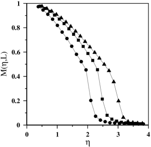
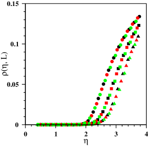
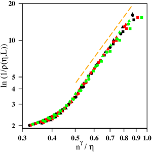
(a)	(b)	(c)

Figure 18: (Color online) The behavior of different quantities against noise for lattice sizes L = 32 (black), 64 (red) and 128 (green) with values of $n$ = 2 (circle), 3 (square) and 4 (triangle). (a) The variation of the order parameter $M(\eta,L)$ against noise $\eta$ are shown for $L=128$ and for $n=2$, 3 and 4. (b) The vortex-pair density $\rho(\eta,L)$ against $\eta$. (c) Scaling collapse of $\ln(1/\rho(\eta,L))$ against $n^{\gamma}/\eta$. For the collapse we use $\gamma=0.28$. The dashed straight line, having slope $\alpha$ = 2.68, is a guide for the eye and indicates the power-law nature in the low noise regime.

VIII 8. Summary and Discussion

To summarize, we have studied a simple model of the collective behavior of $N$ interacting mobile agents which travel in the open free space. In this model we have incorporated the observation of the StarFlag experiment which advocates the necessity of using the topological distance instead of the metric distance. Each agent interacts with a group of $n$ selected agents around it who are positioned within an interaction zone. Every agent freshly selects at a certain rate the group of agents within the IZ. The selection criterion is to choose the first $n$ neighbors. In this paper we have studied two limiting situations, i.e., when the refreshing rates are fastest and the slowest. We first studied when the refreshing rate is slowest i.e., when the IZ for each agent is determined at the beginning and is never updated. All the agents follow the interaction rule in Vicsek model. It has been observed that in absence of noise, starting from a small localized region of space the agents gradually spread as time passes, so that after some relaxation time the flock arrives at a stationary state. The most prominent stationary states are the single sink state and the cyclic state. Using numerical methods we claim that the frequencies of occurrence of other stationary states like the distributed sink states, cycloid states and the space-filling states goes to zero as the neighbor number increases to about 8. Beyond $n=8$ only the SSS and CS states dominate. Finally as $n$ approaches the flock size $N$, only the SSS states dominate.

Interestingly, it has also been observed that the actual metric distances of the $n$ topological neighbors do not become arbitrarily large in all these stationary states in absence of noise. For the SSS states it is true exactly. For the Cyclic states also the topological neighbors remain within a finite distance from an agent (see Fig. 12). Moreover, when the refreshing rate is the fastest, every fragmented cluster travels in a single sink state. Therefore, it is this close proximity of the neighbors that gives rise to the cohesiveness present in our model.

Further, on the application of noise a crossover takes place from the ballistic motion to the diffusive motion and the crossover time depends on the strength of the noise $\eta$, which diverges as $\eta\to 0$. Further the calculation of the Order Parameter $M(\eta)$ and the Binder cumulant $G(\eta)$ lead us to estimate the critical noise $\eta_{c}$ required for the continuous transition from the ordered to the disordered phase. Secondly, when the refreshing rate is fastest, each agent freshly determines its neighbors in the interaction zone at every time step. In the stationary state the flock gets fragmented into a number of smaller clusters of different sizes. The agents in a cluster move completely coherently, different cluster has different direction of motion.

A simpler version of the model has also been studied in the limit of the speed $v\to 0$ when the positions of spins are completely frozen at the sites of a square lattice, but their orientational angles $\theta_{i}(t)$ evolve with time again by the Vicsek interaction. Here for $n$ = 4 the spin configuration is completely static. On the other hand for $n$ = 2 and 3, the entire spin configuration moves along the diagonal and parallel to the asymmetry axis respectively. Further we have observed that the density of vortex-antivortex pairs increases with the strength of the noise and fits to a nice finite-size scaling behavior.

Overall, our findings suggest that complex spatio-temporal patterns may emerge in the interplay between an underlying network structure and collective motion. We believe that our study would also be relevant in the general problem of consensus development in networked agents Olfati-Saber and as such issues like undesired synchronization observed in real-world networks sally-floyd . We observed that multiple frequencies develop during oscillations of different dynamical variables. Whether there is a possibility that a cascade of frequencies develop eventually leading to chaotic behavior remains an open question.

IX Acknowledgment

Useful discussion with Shraddha Mishra is thankfully acknowledged. K.B. acknowledges the support from the BITS Research Initiation Grant Fund.

References

- (1) Reynolds, C. W. (1987), Flocks, herds and schools: A distributed behavioral model, Computer Graphics, 21, 25-34.
- (2) Vicsek, T. and Zafeiris, A. (2012), Collective motion, Phys. Rep., 517, 71-140.
- (3) Toner, J. and Tu, Y. (1995), Long-Range Order in a Two-Dimensional Dynamical XY Model: How Birds Fly Together, Phys. Rev. Lett., 75, 4326-4329.
- (4) Buhl, J., Sumpter, D. J. T., Couzin, I. D., Hale, J. J., Despland, E., Miller, E. R., and Simpson, S. J. (2006), From disorder to order in marching locusts, Science, 312, 1402-1406.
- (5) Nagy, M., Ákos, Z., Biro, D., and Vicsek, T. (2010), Hierarchical group dynamics in pigeon flocks, Nature, 464, 890-893.
- (6) Croft, D. P., Arrowsmith, B. J., Bielby, Skinner, K., White, E., Couzin, I. D., Magurran, A. E., Ramnarine, I., and Krause, J. (2003), Mechanisms underlying shoal composition in the Trinidadian guppy, Poecilia reticulata, Okios, 100, 429.
- (7) Moussaïd, M., Perozo, N., Garnier, S., Helbing, D., and Theraulaz, G. (2010), The Walking Behaviour of Pedestrian Social Groups and Its Impact on Crowd Dynamics, PLoS ONE, 5, e10047.
- (8) Vicsek, T., Czirók, A., Ben-Jacob, E., Cohen, I., and Shochet, O. (1995), Novel Type of Phase Transition in a System of Self-Driven Particles, Phys. Rev. Lett., 75, 1226-1229.
- (9) Grégoire, G. and Chaté, H. (2004), Onset of Collective and Cohesive Motion, Phys. Rev. Lett., 92, 025702-025705.
- (10) Chaté, H., Ginelli, F., Grégoire, G., and Raynaud, F. (2008), Collective motion of self-propelled particles interacting without cohesion, Phys. Rev. E., 77, 046113-046127.
- (11) Ballerini, M., Cabibbo, N., Candelier, R., Cavagna, A., Cisbani, E., Giardina, I., Lecomte, V., Orlandi, A., Parisi, G., Procaccini, A., Viale, M., and Zdravkovic, V. (2008), Interaction ruling animal collective behavior depends on topological rather than metric distance: Evidence from a field study, Proc. Natl. Acad. Sci., 105, 1232-1237.
- (12) Gautrais, J., Ginelli, F., Fournier, R., Blanco, S., Soria, M., Chaté, H., Theraulaz, G. (2012), Deciphering Interactions in Moving Animal Groups, PLoS Comput. Biol., 8, e1002678.
- (13) Ginelli, F. and Chateé, H. (2010), Relevance of Metric-Free Interactions in Flocking Phenomena, Phys. Rev. Lett., 105, 168103-168106.
- (14) Peshkov, A., Ngo, S., Bertin, E., Chaté, H., and Ginelli, F. (2012), Continuous Theory of Active Matter Systems with Metric-Free Interactions Phys. Rev. Lett., 109, 098101-098106.
- (15) Heupe, C. and Aldana, M. (2008), New tools for characterizing swarming systems: A comparison of minimal models, Physica A, 387, 2809-2822.
- (16) Jadbabaie, A., Lin, J., and Morse, A. S. (2003), Coordination of groups of mobile autonomous agents using nearest neighbor rules, Automatic Control, IEEE Transactions, 48, 988-1001.
- (17) Tanner, H. G., Jadbabaie, A., and Pappas, G. J. (2003), Stable flocking of mobile agents, part I: fixed topology, Proceedings of the 42nd IEEE Conference on Decision and Control, 2, 2010-2015.
- (18) Bode, N. W. F., Wood, A. J., and Franks, D. W. (2011), The impact of social networks on animal collective motion, Anim. Behav., 82, 29-38.
- (19) Chaté, H., Ginelli, F., and Montagne, R. (2006), Simple Model for Active Nematics: Quasi-Long-Range Order and Giant Fluctuations, Phys. Rev. Lett., 96, 180602-180605.
- (20) Dall, J. and Christensen, M. (2002), Random geometric graphs, Phys. Rev. E, 66, 016121-016129.
- (21) Herrmann, H.J., Hong, D.C., and Stanley, H.E. (1984), Backbone and elastic backbone of percolation clusters obtained by the new method of “burning”, J. Phys. A, 17, L261-L266.
- (22) Nagy M., Daruka I. and Vicsek T. (2007), New aspects of the continuous phase transition in the scalar noise model (SNM) of collective motion, Physica A, 373, 445-454.
- (23) Kosterlitz, J. M. and Thouless, D. J. (1973), Ordering, metastability and phase transitions in two-dimensional systems, J. Phys. C, 60, 1181-1203.
- (24) Toner, J., Tu, Y., Ramaswamy, S., (2005), Hydrodynamics and phases of flocks, Annals of Physics, 318, 170–244.
- (25) Miyashita, S., Nishimori, H., Kuroda, A., and Suzuki, M. (1978), Monte Carlo Simulation and Static and Dynamic Critical Behavior of the Plane Rotator Model, Prog. Theor. Phys., 60, 1669-1685.
- (26) Tobochnik, J. and Chester, G. V. (1979), Monte Carlo study of the planar spin model, Phys. Rev. B, 20, 3761-3769.
- (27) Olfati-Saber, R. and Murray, R. M. (2007), Consensus and Cooperation in Networked Multi-Agent Systems, Proceedings of the IEEE, 95, 215-233.
- (28) Floyd, S. (1994), The Synchronization of Periodic Routing Messages, IEE/ACM TRANSACTIONS ON NETWORKING, 2, 122-136.