Impurity entanglement through electron scattering in a magnetic field

Abstract

We study the entanglement of magnetic impurities in an environment of electrons through successive scattering while an external magnetic field is applied. We show that the dynamics of the problem can be approximately described by a reduced model of three interacting spins, which reveals an intuitive view on how spins can be entangled by controlled electron scattering. The role of the magnetic field is rather crucial. Depending on the initial state configuration, the magnetic field can either increase or decrease the resulting entanglement but more importantly it can allow the impurities to be maximally entangled.

The past few years have seen a large explosion of interest in the studies of the interfaces between quantum information and many body systems. The controlled production and detection of entangled particles is the first step on the road towards quantum information processing nielsen2000quantum . A variety of methods to entangle electrons or localized spins have been proposed, based on quite different physical mechanisms PhysRevB.61.R16303 ; PhysRevLett.84.1035 ; PhysRevLett.88.037901 ; PhysRevLett.90.166803 ; PhysRevB.63.165314 ; PhysRevB.65.165327 ; PhysRevLett.89.037901 ; PhysRevLett.87.277901 ; PhysRevLett.91.157002 ; PhysRevB.69.235312 ; PhysRevLett.91.147901 ; springerlink ; PhysRevLett.96.230501 ; PhysRevB.74.153308 ; PhysRevA.81.042318 ; RKKY_Cho . One particular straight-forward application is the generation of entanglement between magnetic impurities or localized spins in mesoscopic structures PhysRevLett.96.230501 ; PhysRevB.74.153308 ; PhysRevA.81.042318 ; RKKY_Cho , e.g. by means of electron scattering. For the purpose of studying controlled entanglement between localized qubits one can imagine an experimental realization with the help of coupled quantum dots PhysRevA.57.120 , which contain electrons that have relatively long relaxation times PhysRevB.76.035315 and where coherent manipulations are possible Nature.453.1043 . Moving quantum dots generated by surface acoustic waves barnes have also been observed experimentally SAW_Kataoka and proposed as candidates for quantum computation SAW_Shi . The controlled insertion of single impurity atoms with two hyperfine states (qubits) in a bath of ultra-cold atoms has also become an active field of research widera . The basic idea of an indirect coupling between localized spins is not new and has first been considered many years ago in the context of localized nuclear or electron spins that can couple to conduction electrons, leading to the so–called Ruderman–Kittel–Kasuya–Yosida (RKKY) interaction RKKY . However, in order to study entanglement, an effective RKKY coupling alone is not enough as we will show.

In the present work, we consider a minimal model of two localized spins (qubits) that are coupled indirectly via an environment in which electrons are injected and couple to both spins as depicted in Fig. 1 (left). In particular, we are interested in the dynamics of the entanglement of the two qubits after an electron is injected into the lattice with a given initial state. In addition, an external magnetic field is applied on the system as a control mechanism over the generated entanglement. Even though an effective RKKY interaction alone is not sufficient to explain the entanglement dynamics, it is sometimes possible to use a simplified model of only three interacting spins, Fig. 1 (right), exemplifying the entanglement mechanism as well as the important role of the magnetic field maximizing or destroying entanglement.

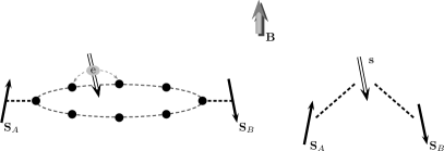
Figure 1: (left) Two embedded impurities in a ring are entangled via successive electron scattering. In addition an external magnetic field is applied. (right) A minimal model of three interacting spins.

The Hamiltonian describing this mechanism consists of electrons with kinetic energy ${H_{0}}$, the interaction with localized spins $V$ and the coupling to a magnetic field $H_{B}$ PhysRevLett.96.230501 ; PhysRevB.74.153308

$$H = {H_{0}}+V+H_{B}$$

$$= \sum_{k,\sigma}\epsilon_{k}a_{k,\sigma}^{\dagger}a_{k,\sigma}+J~{}(\mathbf{s}_{0}\cdot\mathbf{S}_{\mathrm{A}}+\mathbf{s}_{N}\cdot\mathbf{S}_{\mathrm{B}})+B\sum_{l}s^{z}_{l}~{}.$$

Here, $0,N$ are the positions of localized spins $\mathbf{S}_{\mathrm{A}}$ and $\mathbf{S}_{\mathrm{B}}$, which we will call impurities in a system of total length $L$—note that there is no direct interaction between the impurities. The electron spin is expressed in terms of creation $a^{\dagger}$, annihilation $a$ operators $\mathbf{s}_{l}=\frac{1}{2}\sum_{\alpha,\beta}a^{\dagger}_{l,\alpha}{\bm{\sigma}}_{\alpha\beta}a_{l,\beta}$, with ${\bm{\sigma}}$ the Pauli matrices. Furthermore, we work in units of $J$ by setting the lattice constant $a=1$, Planck’s constant $\hbar=1$ and Bohr’s magneton $\mu_{B}=1$. The hopping amplitude of the one–dimensional tight binding Hamiltonian is given by ${\tilde{t}}$, viz. $\epsilon_{k}=-2{\tilde{t}}\cos k$, $k=\left(2\pi/L\right)n$ with $n=-L/2,\ldots,L/2-1$.

One of the most important symmetries of Hamiltonian (Impurity entanglement through electron scattering in a magnetic field) is the conservation of the total $S^{z}=s^{z}+S_{\mathrm{A}}^{z}+S_{\mathrm{B}}^{z}$ component, which makes it possible to consider an effective field on the electrons only in Eq. (Impurity entanglement through electron scattering in a magnetic field). In particular, a general magnetic field $\mathcal{B}$ applied on all three spins results in a Zeeman interaction of the form $\mathcal{B}[g_{\mathrm{e}}s^{z}+g_{\mathrm{I}}(S_{\mathrm{A}}^{z}+S_{\mathrm{B}}^{z})]=\mathcal{B}(g_{\mathrm{e}}-g_{\mathrm{I}})s^{z}+g_{\mathrm{I}}\mathcal{B}S^{z}$, where $g_{\mathrm{e}}$ and $g_{\mathrm{I}}$ stand for the electron and impurity $g$–factors which in principle are not equal. Since $[H,S^{z}]=0$ the field on the total spin $S^{z}$ does not influence the time evolution and only the effective magnetic field $B=\mathcal{B}(g_{\mathrm{e}}-g_{\mathrm{I}})$ on the electrons has to be considered. If the two $g$–factor were equal $g_{\mathrm{e}}=g_{\mathrm{I}}$ the magnetic field would have no effect on the dynamics of the system.

The generated entanglement between the impurities via the electron spin will acquire a time evolution according to the time evolution of the initial state $|\psi_{0}\rangle$. Among the various quantities that one can extract information for the entanglement of the impurities is the concurrence PhysRevLett.80.2245 ; PhysRevA.63.052302 , a pairwise measure of entanglement. The concurrence between the two impurity spins is related to the reduced density matrix $\varrho(t)=\mathrm{Tr}_{\mathrm{e}}~{}|\psi(t)\rangle\langle\psi(t)|$, where the electron’s degrees of freedom are traced out. Taking into account the symmetries of the Hamiltonian the concurrence of the two impurities in the natural basis $\{|\!\uparrow\uparrow\rangle,|\!\downarrow\uparrow\rangle,|\!\uparrow\downarrow\rangle,|\!\uparrow\uparrow\rangle\}$ reads PhysRevA.69.022304 ; PhysRevB.78.224413

$$\mathcal{C}(t)=2|\varrho_{\downarrow\uparrow,\uparrow\downarrow}(t)|.$$ (2)

In order to gain a basic understanding of the entanglement mechanism, it is useful to first analyze a reduced model of only three coupled spins in a magnetic field, essentially obeying the same symmetries as schematized in Fig. 1 (right)

$$H_{3\mathrm{S}} = {\tilde{J}}\mathbf{s}\cdot(\mathbf{S}_{\mathrm{A}}+\mathbf{S}_{\mathrm{B}})+Bs^{z}~{}.$$ (3)

The evolution of the initial state $|\psi_{0}\rangle=|\sigma_{\mathrm{A}},\sigma_{\mathrm{B}},\sigma_{\mathrm{e}}\rangle$, with $\sigma_{\mathrm{e,A,B}}=\uparrow,\downarrow$, under Hamiltonian (3) at time $t$ is given by $|\psi(t)\rangle=\exp\left(iH_{3\mathrm{S}}t\right)|\psi_{0}\rangle$ and spans the same $S^{z}$ subsector with $|\psi_{0}\rangle$. In the fully polarized one–dimensional $S^{z}=\pm 3/2$ subsectors, the impurities are in a product state and therefore non–entangled at all times $t\geq 0$. Hence, only the $S^{z}=\pm\frac{1}{2}$ subsectors are relevant for entanglement generation between the impurities. We only consider the sector $S^{z}=+\frac{1}{2}$, since the spin-flipped states have the same time evolution for $B\to-B$.

To evaluate the concurrence of the minimal three–spin model we diagonalize analytically $H_{3\mathrm{S}}$ within the $S^{z}=+\frac{1}{2}$ subsector. Then, we find the time evolution of the initial state $|\psi_{0}\rangle$ and evaluate the reduced density matrix $\varrho(t)$ which gives the time evolution of the concurrence using Eq. (2). In the the sector $S^{z}=+\frac{1}{2}$ there are two initial states of interest $|\psi_{0}\rangle=|\!\!\uparrow\uparrow\downarrow\rangle$ and $|\psi_{0}\rangle=|\!\!\uparrow\downarrow\uparrow\rangle$. The corresponding concurrences $\mathcal{C}_{\uparrow\uparrow}(t)$ and $\mathcal{C}_{\uparrow\downarrow}(t)$ evolve according to

$$\mathcal{C}_{\uparrow\uparrow}(t) = \mathcal{A}_{\uparrow\uparrow}\sin^{2}\omega t~{},$$ (4a)

$$\mathcal{C}_{\uparrow\downarrow}(t) = \mathcal{A}_{\uparrow\downarrow}\sqrt{\mathcal{C}_{\uparrow\uparrow}^{2}(t)+4\left(\mathcal{C}_{1}(t)-\frac{\Omega}{\omega}\mathcal{C}_{2}(t)\right)^{2}}~{},$$ (4b)

where $\mathcal{A}_{\uparrow\uparrow}=\frac{{\tilde{J}}^{2}}{2\omega^{2}}$, $\mathcal{A}_{\uparrow\downarrow}=1/2$, $\Omega={\tilde{J}}/4+B/2$, $\omega=\sqrt{{\tilde{J}}^{2}/2+\Omega^{2}}$, $\mathcal{C}_{1}(t)=\sin\Omega t\cos\omega t$, and $\mathcal{C}_{2}(t)=\sin\omega t\cos\Omega t$. The time dependence of the concurrence is controlled by the two frequencies $\omega$ and $\Omega$ which are asymmetric under sign change of the magnetic field; hence the amplitude of $\mathcal{C}_{\uparrow\uparrow}$ is also asymmetric. The competition of two energy scales, namely ${\tilde{J}}$ and $B$ and the choice of initial conditions makes the two directions of the magnetic field $\pm\hat{z}$ not equivalent.

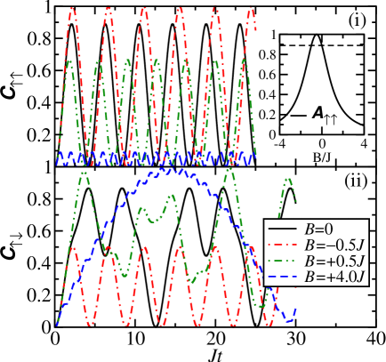
Figure 2: (color online) Entanglement dynamics (concurrence) of the two impurities within model (3) for initially aligned $\mathcal{C}_{\uparrow\uparrow}(t)$ (top), anti–aligned $\mathcal{C}_{\uparrow\downarrow}(t)$ (bottom) impurities and different values of the applied magnetic field. Top inset: Amplitude $\mathcal{C}_{\uparrow\uparrow}$ versus the magnetic field.

The concurrence $\mathcal{C}_{\uparrow\uparrow}(t)$ is plotted in Fig. 2(i) for different values of the applied magnetic field. For initially aligned impurities, the concurrence $\mathcal{C}_{\uparrow\uparrow}(t)$ simply oscillates with a frequency $\omega$. In the absence of magnetic field, concurrence is bounded to $8/9$ [marked with the dashed line in the inset of Fig. 2(i)] while when the magnetic field is switched on the amplitude takes on the maximum value of unity for $\Omega=0$, i.e. $B=-{\tilde{J}}/2$. Furthermore, the applied magnetic field on the electron enhances entanglement between the impurities for $-1<B/{\tilde{J}}<0$ while it reduces entanglement outside this range [see inset in Fig. 2(i)].

For initially anti-aligned impurity spins the behavior of $\mathcal{C}_{\uparrow\downarrow}(t)$ becomes much more interesting as shown in Fig. 2(ii). Due to the two oscillating factors in Eq. (4b) the magnetic field allows the impurities now to be almost maximally entangled $\mathcal{C}_{\uparrow\downarrow}\rightarrow 1$. For times $\omega t_{n}={\pi}n$ when $\mathcal{C}_{\uparrow\uparrow}$ and $\mathcal{C}_{2}$ vanish, $\mathcal{C}_{\uparrow\downarrow}(t_{n})$ has a local maximum with amplitude

$$\mathcal{C}_{\uparrow\downarrow}(t_{n})=|\sin\frac{\Omega}{\omega}\pi n|~{},~{}~{}n=1,2,\ldots~{}~{}.$$ (5)

For increasing $n$ (larger times), one of those local maxima will become a global maximum with a value very close to one, see for example in Fig. 2 the case for $B=+0.5{\tilde{J}}$ and $t=6\pi/\omega\approx 21.8/{\tilde{J}}$. Note that a necessary condition for this to happen is the irrational value of the ratio $\Omega/\omega$. Moreover, for an irrational value of $\Omega/\omega$ the concurrence $\mathcal{C}_{\uparrow\downarrow}(t>0)$ remains strictly larger than zero, so the impurities are entangled for any $t>0$.

So far we have seen that $\mathcal{C}_{\uparrow\uparrow}(t)$, $\mathcal{C}_{\uparrow\downarrow}(t)$ show a fundamentally different time evolution for any value of $B$. It is instructive to consider the origin of these asymmetries as a consequence of statistical considerations. At small times, transition rates are given in terms ${w_{\alpha\rightarrow\beta}}=\langle\alpha|\left(\mbox{1I}-iH\Delta t\right)|\beta\rangle$. It is then straight-forward to see that for $B\neq 0$ the probabilities ${P_{\alpha\rightarrow\beta}}=|{w_{\alpha\rightarrow\beta}}|^{2}$ differ depending on the initial state and the direction of the magnetic field. For example, ${P_{\uparrow\uparrow\rightarrow\downarrow\uparrow}}$ will be larger than ${P_{\downarrow\uparrow\rightarrow\uparrow\uparrow}}$ for $B>0$. Furthermore, for a given initial state, one can see that the concurrence will exhibit an asymmetric behavior with respect to the direction of the magnetic field.

Let us now consider the more realistic model depicted in Fig. 1(left), obeying essentially the same symmetries as model (3). Here, the magnetic impurities $\mathbf{S}_{\mathrm{A}}$ and $\mathbf{S}_{\mathrm{B}}$ are embedded respectively at sites $0,N$ PhysRevLett.96.230501 ; PhysRevB.74.153308 . An electron is injected into the lattice, with a given initial state, and scatters off the impurities. The initial state will be of the form $|\uparrow\uparrow\downarrow_{k}\rangle$ where the index $k$ is introduced to describe electron’s momentum and the evolution of the initial state occurs under Hamiltonian (Impurity entanglement through electron scattering in a magnetic field). Note that the electron is considered to initially occupy an eigenstate of $H_{0}$ with momentum $k$.

We now focus on the time evolution of the states $|\uparrow\uparrow\downarrow_{k}\rangle$, $|\downarrow\uparrow\uparrow_{k}\rangle$ and $|\uparrow\downarrow\uparrow_{k}\rangle$ (spanning the subsector $S^{z}_{\mathrm{total}}=1/2$) under Hamiltonian (Impurity entanglement through electron scattering in a magnetic field). To implement the time evolution of the states we consider the time evolution of the spinor

$${\widetilde{\Gamma}}_{k}^{\dagger}=\left({\Gamma^{\dagger}_{\uparrow\uparrow,\downarrow}}_{k}~{},{\Gamma^{\dagger}_{\downarrow\uparrow,\uparrow}}_{k}~{},{\Gamma^{\dagger}_{\uparrow\downarrow,\uparrow}}_{k}~{}\right),~{}~{}{\Gamma^{\dagger}_{\alpha\beta,\tau}}_{k}=f^{\dagger}_{0,\alpha}f^{\dagger}_{N,\beta}a^{\dagger}_{\tau,k}~{},$$

where the fermionic operator $f^{\dagger}_{m,\alpha}$ creates the impurity on site $m$ with spin $\alpha$. Application of the spinor ${\Gamma^{\dagger}_{\alpha\beta,\tau}}_{k}$ onto the vacuum generates an initial state with the corresponding parameters. After Laplace transforming the time evolution we obtain

$$\left(z-{\mathcal{H}_{0}}\right){\widetilde{\Gamma}}_{k}^{\dagger}(z)={\widetilde{\Gamma}}_{k}^{\dagger}(0)+\sum_{q}\left(\mathcal{V}_{k,q}+\mathcal{H}_{b,k,q}\right){\widetilde{\Gamma}}_{q}^{\dagger}(z),$$ (6)

where $z$ stands for the Laplace frequencies and the $3\times 3$ matrices ${\mathcal{H}_{0}}$, $\mathcal{V}_{k,q}$ and $\mathcal{H}_{b,k,q}$ are derived from the application of $H_{0}$, $V$ and $H_{B}$ on the spinor ${\widetilde{\Gamma}}_{k}^{\dagger}$ respectively.

To further proceed with the solution of the system of self-consistent equation (6) we may apply a resonant coupling approximation as proposed in Ref. PhysRevB.74.153308 . That is, due to resonance, only terms with $q=\pm k$ (degenerate eigenstates of ${H_{0}}$) are relevant and we end up with a system of equations coupling only the spinors with wave vectors $k$ and $-k$. This system can be reversed if we merge the spinors ${\widetilde{\Gamma}}_{k}^{\dagger}(z)$ and ${\widetilde{\Gamma}}_{-k}^{\dagger}(z)$ to form a new spinor ${\widetilde{\Psi}^{\dagger}}_{k}(z)$ satisfying

$${\widetilde{\Psi}^{\dagger}}_{k}(z)=\left(\begin{tabular}[]{c c}$\mathcal{W}_{k,k}$&$-\mathcal{V}_{k,-k}$\\ $-\mathcal{V}_{-k,k}$&$\mathcal{W}_{-k,-k}$\end{tabular}\right)^{-1}{\widetilde{\Psi}^{\dagger}}_{k}(0)~{},$$ (7)

with $\mathcal{W}_{k,k}=z-{\mathcal{H}_{0}}-\mathcal{V}_{k,k}-\mathcal{H}_{b,k,k}$. Lastly, as was shown in Ref. PhysRevB.74.153308 , the system of equations (7) simplifies drastically if one selects a commensurate value of the product $kN$, namely $kN=\pi\times\mathrm{integer}$. The time evolution of an initial state $|\psi_{0}\rangle$ is obtained after inverse Laplace transform Eq. (7) and the concurrence using Eq. (2) after tracing out electron’s degrees of freedom.

For $|\psi_{0}\rangle=\mbox{$|\uparrow\uparrow\downarrow_{k}\rangle$}$, we arrive at Eq. (4a) for $\mathcal{C}_{\uparrow\uparrow}(t)$ with an amplitude $\mathcal{A}_{\uparrow\uparrow}=(2J/L)^{2}/4\omega^{2}$ and the two frequencies $\Omega=(2J/L)/4+B/2$, $\omega=\sqrt{(2J/L)^{2}/2+\Omega^{2}}$. For $|\psi_{0}\rangle=\mbox{$|\uparrow\downarrow\uparrow_{k}\rangle$}$, we arrive at Eq. (4b) for $\mathcal{C}_{\uparrow\downarrow}(t)$ with $\mathcal{A}_{\uparrow\downarrow}=1/4$. Thus, at resonance, the entanglement dynamics of the lattice is the same with the one of the 3–spin model with reduced amplitudes $\mathcal{A}_{\uparrow\uparrow}$ and $\mathcal{A}_{\uparrow\downarrow}$ by a factor of two and an effective coupling ${\tilde{J}}=2J/L$ between electron and impurities driving the oscillations. The origin for the difference in the amplitude of the concurrence between the 3–spin model (3) and the full model (Impurity entanglement through electron scattering in a magnetic field) arises from the scattering into different momentum channels for the latter. Particularly in this case, it is the backscattering that bounds the concurrence to $1/2$, prohibiting maximum entanglement $\mathcal{C}\rightarrow 1$. In fact, it is possible to consider a symmetric or anti-symmetric linear combination of degenerate plane waves with opposite momentum $k$ and $-k$. For the symmetric (cosine) initial condition the amplitude of the concurrence is doubled resulting in maximum entanglement at times $\omega t_{m}=\pi(m+1/2)$, while for the anti-symmetric linear combination no entanglement takes place.

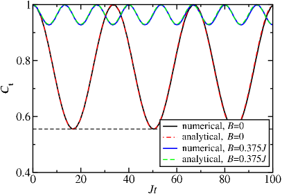
Figure 3: (color online) Entanglement dynamics (concurrence) $\mathcal{C}_{\mathrm{t}}(t)$ of the full model (Impurity entanglement through electron scattering in a magnetic field) with $\tilde{t}=5J$ and $L=16$ for two values of the magnetic field $B=0$ and $B=0.375J$. The dashed line indicates the minimum of entanglement in the absence of magnetic field.

To test our analytical calculation, we study numerically the time evolution of Hamiltonian (Impurity entanglement through electron scattering in a magnetic field) using exact diagonalization (ED). We consider initially entangled impurities in a singlet $|\psi_{0}\rangle=\frac{1}{\sqrt{2}}\left(|\downarrow\uparrow\uparrow_{k}\rangle-|\uparrow\downarrow\uparrow_{k}\rangle\right)$ or triplet $|\psi_{0}\rangle=\frac{1}{\sqrt{2}}\left(|\downarrow\uparrow\uparrow_{k}\rangle+|\uparrow\downarrow\uparrow_{k}\rangle\right)$ combination. The corresponding $\mathcal{C}_{\mathrm{s}}$ and $\mathcal{C}_{\mathrm{t}}$ concurrence for the singlet and the triplet configuration are given by

$$\mathcal{C}_{\mathrm{s}}(t)=1~{},\qquad\mathcal{C}_{\mathrm{t}}(t)=1-\mathcal{C}_{\uparrow\uparrow}(t)~{}.$$ (8)

Remarkably, impurities in a singlet combination remain maximally entangled at all $t\geq 0$. This is easily understood within the 3–spin model where the singlet configuration is an eigenstate of $H_{3\mathrm{S}}$ leading to a time independent concurrence. On the other hand, the triplet initial state exhibits a sinusoidal behavior, shown in Fig. 3. For the triplet initial state, deviation from maximum entanglement occurs due to the oscillating term, the amplitude of which reduces for magnetic fields outside the range $-1<B/{\tilde{J}}<0$, see inset in Fig. 2(i). Therefore, any positive or strong negative magnetic field applied on the electron can significantly enhance entanglement between impurities.

In addition in Fig. 3, we plot numerical results obtained via ED for system size $L=16$, impurity distance $N=4$, and an electron in the state $k=\pi/2$. Numerical and analytical results are in very good agreement for $\mathcal{C}_{\mathrm{t}}$ and consequently for $\mathcal{C}_{\uparrow\uparrow}$ and $\mathcal{C}_{\uparrow\downarrow}$, as long as the scattering of the electron on the impurities is relatively weak. For stronger $J$, namely for $J/L$ comparable to the distance between the single particle energy levels, a wider range of scattering states participate. In this regime, the kinetic degrees of freedom become more important and interference of scattering into different momenta leads to non trivial entanglement dynamics. The resonance approximation breaks down and naturally the minimal 3–spin model fails to capture the entanglement process too.

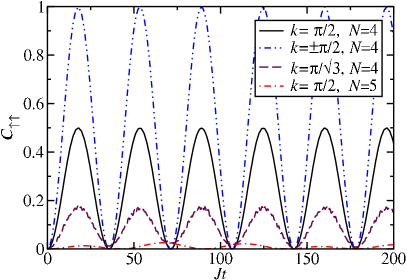
Figure 4: (color online) Entanglement dynamics of the full model (Impurity entanglement through electron scattering in a magnetic field) with $L=16$ for two initially aligned impurities obtained via numerical diagonalization for different electron initial states (see text) and impurity distances $N$. The magnetic field is chosen $B=-J/L$, so that $\Omega=0$.

So far, we have focused on the generated entanglement between the impurities considering different spin configurations and the influence of the magnetic field. Let us now work on a different scenario where the entanglement is tuned by other parameters like the impurity distance $N$ or the initial spatial part of electron’s wave function. To realize this, we work in the $S^{z}=1/2$ subsector for initially aligned impurities in a system of $L=16$ sites and a fixed magnetic field $B=-J/L$ which corresponds to $\Omega=0$, where maximal amplitudes are possible. In Fig. 4, we plot four characteristic examples. First, we plot the case where the electron is injected in the state $k=\pi/2$ and the impurities are $N=4$ sites apart. As discussed above the entanglement dynamics is well described by Eq. (4a) in this case, exhibiting a simple sinusoidal form with half of the maximum amplitude. If an electron is injected in a symmetric (cosine) superpositions of states $k=\pm\pi/2$ (second case) a maximum amplitude and maximal entanglement can indeed be obtained, as also discussed above. More interesting is a more generic case where an electron is injected into the state $k=\pi/\sqrt{3}$, which is not an eigenstate of ${H_{0}}$. In this third case, we observe a suppression of the overall amplitude and very fast oscillations on top of the dominant sinusoidal form. This pattern results from the fact that states with different energies contribute to the entanglement now, but nonetheless it is remarkable that the dominant sinusoidal form remains in agreement with a simple three spin model. The same is also true for an incommensurate distance $N=5$ between the impurities (forth case). The signal is now a suppressed superposition of oscillations with a different dominant frequency. Nonetheless, an interpretation of such generic cases with the help of three spin models is in principle possible by taking the frequencies and amplitudes as fitting parameters.

Finally, let us discuss the possibility of an RKKY description of Hamiltonian (Impurity entanglement through electron scattering in a magnetic field). We have shown that the three-spin model in Eq. (3) contains essential features for the entanglement dynamics of the impurities. This contradicts the possibility of an RKKY description of Hamiltonian (Impurity entanglement through electron scattering in a magnetic field) due to the different geometries of an RKKY Hamiltonian and Hamiltonian (3). Specifically, the RKKY Hamiltonian will be given by $H=\mathcal{J}(N)\mathbf{S}_{\mathrm{A}}\cdot\mathbf{S}_{\mathrm{B}}$ with $\mathcal{J}(N)$ some effective coupling depending on the distance between the impurities. The failure of such a description becomes apparent if one considers the initial impurity configuration $|\!\uparrow\uparrow\rangle$ which is a separable state and an eigenstate of the RKKY interaction, resulting to zero entanglement at all times, $\mathcal{C}_{\uparrow\uparrow}(t)=0$. On the other hand, the configuration $|\!\uparrow\downarrow\rangle$, which has overlap to two eigenstates of the RKKY Hamiltonian, gives an oscillating behavior for the entanglement of the form $\mathcal{C}_{\uparrow\downarrow}(t)=|\sin\mathcal{J}t|$, which is qualitatively different from the one we found for model (Impurity entanglement through electron scattering in a magnetic field).

In conclusion, we have studied the entanglement of two magnetic spin-$\frac{1}{2}$ impurities embedded in a tight binding ring in the presence of magnetic field. We showed that the main aspects of the time evolution of the entanglement between the impurities is revealed by a simplified model of three spins, Eq. (3), valid for small coupling $J$ and magnetic field $B$, disproving the possibility of an effective RKKY description. Moreover, we solved analytically the full model, Eq. (Impurity entanglement through electron scattering in a magnetic field), using a resonance approximation and obtained analytical formulas for various initial spin configurations. As far as the role of the magnetic field is concerned, we have shown that it can be used as a control mechanism over the generated entanglement. Finally, the generated entanglement is largely affected by the spatial part of electron’s wavefunction as well as the position of the impurities in the lattice.

- (1) M. Nielsen, I. Chuang, Quantum computation and quantum information (Cambridge Univeristy Press, 2000).
- (2) G. Burkard, D. Loss, E.V. Sukhorukov, Phys. Rev. B 61, R16303 (2000).
- (3) D. Loss, E.V. Sukhorukov, Phys. Rev. Lett. 84, 1035 (2000).
- (4) W.D. Oliver, F. Yamaguchi, Y. Yamamoto, Phys. Rev. Lett. 88, 037901 (2002).
- (5) D.S. Saraga, D. Loss, Phys. Rev. Lett. 90, 166803 (2003).
- (6) P. Recher, E.V. Sukhorukov, D. Loss, Phys. Rev. B 63, 165314 (2001).
- (7) P. Recher, D. Loss, Phys. Rev. B 65, 165327 (2002).
- (8) C. Bena, S. Vishveshwara, L. Balents, M.P.A. Fisher, Phys. Rev. Lett. 89, 037901 (2002).
- (9) A.T. Costa, S. Bose, Phys. Rev. Lett. 87, 277901 (2001).
- (10) P. Samuelsson, E.V. Sukhorukov, M. Büttiker, Phys. Rev. Lett. 91, 157002 (2003); Phys. Rev. Lett. 92, 026805 (2004).
- (11) A.V. Lebedev, G. Blatter, C.W.J. Beenakker, G.B. Lesovik, Phys. Rev. B 69, 235312 (2004).
- (12) C.W.J. Beenakker, C. Emary, M. Kindermann, J.L. vanVelsen, Phys. Rev. Lett. 91, 147901 (2003).
- (13) G. Lesovik, T. Martin, G. Blatter, Eur. Phys. J. B 24, 287 (2001).
- (14) A.T. Costa, S. Bose, Y. Omar, Phys. Rev. Lett. 96, 230501 (2006).
- (15) G.L. Giorgi, F. dePasquale, Phys. Rev. B 74, 153308 (2006).
- (16) F. Ciccarello, S. Bose, M. Zarcone, Phys. Rev. A 81, 042318 (2010).
- (17) S.Y. Cho, R.H. McKenzie, Phys. Rev. A 73, 012109 (2006).
- (18) D. Loss, D.P. DiVincenzo, Phys. Rev. A 57, 120 (1998).
- (19) J.M. Taylor, J.R. Petta, A.C. Johnson, A. Yacoby, C.M. Marcus, M.D. Lukin, Phys. Rev. B 76, 035315 (2007).
- (20) R. Hanson, D.D. Awschalom, Nature 453, 1043 (2008).
- (21) C.H.W. Barnes, J.M. Shilton, A.M. Robinson, Phys.Rev. B 62, 8410 (2000).
- (22) M. Kataoka, M.R. Astley, A.L. Thorn, D.K.L. Oi, C.H.W. Barnes, C.J.B. Ford, D. Anderson, G.A.C. Jones, I. Farrer, D.A. Ritchie, M. Pepper, Phys. Rev. Lett. 102, 156801 (2009).
- (23) X. Shi, M. Zhang, L.F. Wei, Phys. Rev. A 84, 062310 (2011).
- (24) N. Spethmann, F. Kindermann, S. John, C. Weber, D. Meschede, and A. Widera Phys. Rev. Lett. 109, 235301 (2012).
- (25) M.A. Ruderman and C. Kittel, Phys. Rev. 96, 99 (1954); T. Kasuya, Prog. Theor. Phys. 16, 45 (1956); K. Yosida, Phys. Rev. 106, 893 (1957).
- (26) W.K. Wootters, Phys. Rev. Lett. 80, 2245 (1998).
- (27) K.M. O’Connor, W.K. Wootters, Phys. Rev. A 63, 052302 (2001).
- (28) L. Amico, A. Osterloh, F. Plastina, R. Fazio, and G. M. Palma Phys. Rev. A 69, 022304 (2004)
- (29) R. Dillenschneider, Phys. Rev. B 78, 224413 (2008)