Bayesian Models of Graphs, Arrays and Other Exchangeable Random Structures

Abstract

The natural habitat of most Bayesian methods is data represented by exchangeable sequences of observations, for which de Finetti’s theorem provides the theoretical foundation. Dirichlet process clustering, Gaussian process regression, and many other parametric and nonparametric Bayesian models fall within the remit of this framework; many problems arising in modern data analysis do not. This article provides an introduction to Bayesian models of graphs, matrices, and other data that can be modeled by random structures. We describe results in probability theory that generalize de Finetti’s theorem to such data and discuss their relevance to nonparametric Bayesian modeling. With the basic ideas in place, we survey example models available in the literature; applications of such models include collaborative filtering, link prediction, and graph and network analysis. We also highlight connections to recent developments in graph theory and probability, and sketch the more general mathematical foundation of Bayesian methods for other types of data beyond sequences and arrays.

I Introduction

For data represented by exchangeable sequences, Bayesian nonparametrics has developed into a flexible and powerful toolbox of models and algorithms. Its modeling primitives—Dirichlet processes, Gaussian processes, etc.—are widely applied and well-understood, and can be used as components in hierarchical models [61] or dependent models [50] to address a wide variety of data analysis problems. One of the main challenges for Bayesian statistics and machine learning is arguably to extend this toolbox to the analysis of data sets with additional structure, such as graph, network, and relational data.

In this article, we consider structured data—sequences, graphs, trees, matrices, etc.—and ask:

What is the appropriate class of statistical models for a given type of structured data?

Representation theorems for exchangeable random structures lead us to an answer, and they do so in a very precise way: They characterize the class of possible Bayesian models for the given type of data, show how these models are parametrized, and even provide basic convergence guarantees. The probability literature provides such results for dozens of exchangeable random structures, including sequences, graphs, partitions, arrays, trees, etc. The purpose of this article is to explain how to interpret these results and how to translate them into a statistical modeling approach.

Overview

TABLE I: Exchangeable random structures

Random structure	Theorem of	Ergodic distributions $\mathbf{p}_{\theta}$	Statistical application
Exchangeable sequences	de Finetti [24, 25]	product distributions	most Bayesian models [e.g. 59]
	Hewitt and Savage [31]
Processes with exchangeable increments	Bühlmann [19]	Lévy processes
Exchangeable partitions	Kingman [41]	“paint-box” distributions	clustering
Exchangeable arrays	Aldous [3]	sampling schemes Eq. VI.4, Eq. VI.10	graph-, matrix- and array-valued
	Hoover [36]		data (e.g., [33]); see Section IV
	Kallenberg [37]
Block-exchangeable sequences	Diaconis and Freedman [21]	Markov chains	e.g. infinite HMMs [10, 26]

Consider a data analysis problem in which observations are represented as edges in a graph. As we observe more data, the graph grows. For statistical purposes, we might model the graph as a sample from some probability distribution on graphs. Can we estimate the distribution or, at least, some of its properties? If we observed multiple graphs, all sampled independently from the same distribution, we would be in the standard setting of statistical inference. For many problems in e.g. network analysis, that is clearly not the approach we are looking for: There is just one graph, and so our sample size should relate to the size of the graph. Of course, we could assume that the edges are independent and identically distributed random variables, and estimate their distribution—that would indeed be a way of performing inference within a single graph. The resulting model, however, is sensitive only to the number of edges in a graph and so has only a single parameter ${p\in[0,1]}$, the probability that an edge is present. What are more expressive models for graph-valued data?

Compare the problem to a more familiar one, where data is represented by a random sequence ${X:=(X_{1},X_{2},\ldots)}$, whose elements take values in a sample space $\mathbf{X}$, and $n$ observations are interpreted as the values of the initial elements ${X_{1},\ldots,X_{n}}$ of the sequence. In this case, a statistical model is a family ${\mathcal{P}=\{P_{\theta}|\theta\in\mathbf{T}\}}$ of distributions on $\mathbf{X}$, indexed by elements $\theta$ of some parameter space $\mathbf{T}$. If the sequence $X$ is exchangeable, de Finetti’s theorem tells us that there is some model $\mathcal{P}$ and some distribution $\nu$ on $\mathbf{T}$ such that the joint distribution of $X$ is

$$\mathbb{P}(X\in\,.\,)=\int_{\mathbf{T}}P_{\theta}^{\infty}(\,.\,)\nu(d\theta)\;.$$ (I.1)

This means the sequence can be generated by first generating a random parameter value ${\Theta\sim\nu}$, and then sampling ${X_{1},X_{2},\ldots|\Theta\sim_{\mbox{\tiny iid}}P_{\Theta}}$. In particular, the elements of the sequence are conditionally i.i.d. given $\Theta$.

For the purposes of statistical inference, the (conditional) i.i.d. structure implies that we can regard the elements $X_{i}$ of the sequence as repetitive samples from an unknown distribution $P_{\Theta}$, and pool these observations to extract information about the value of $\Theta$. This may be done using a Bayesian approach, by making a modeling assumption on $\nu$ (i.e., by defining a prior distribution) and computing the posterior given data, or in a frequentist way, by assuming $\theta$ is non-random and deriving a suitable estimator.

To generalize this idea to the graph case, we regard the infinite sequence ${X:=(X_{1},X_{2},\ldots)}$ as an infinite random structure, of which we observe a finite substructure (the initial segment ${X_{1},\ldots,X_{n}}$). From this perspective, de Finetti’s theorem tells us how to break down a random structure (the sequence) into components (the conditionally independent elements), which in turn permits the definition of statistical inference procedures. What if, instead of an infinite sequence, $X$ is an infinite graph, of which we observe a finite subgraph? To mimic the sequence case, we would need a definition of exchangeability applicable to graphs, and a suitable representation theorem to substitute for de Finetti’s.

Since generating a parameter ${\Theta\sim\nu}$ randomly determines a distribution $P_{\Theta}$, we can think of $P_{\Theta}$ as a random probability measure with distribution defined by $\nu$, and paraphrase de Finetti’s theorem as follows:

The joint distribution of any exchangeable sequence of random values in $\mathbf{X}$ is characterized by the distribution of a random probability measure on $\mathbf{X}$.

If we assume a random graph to be exchangeable—where we put off the precise definition for now—it is indeed also characterized by a representation theorem. The implications for statistical models are perhaps more surprising than in the case of sequences:

The distribution of any exchangeable graph is characterized by a distribution on the space of functions
from $[0,1]^{2}$ to $[0,1]$.

Hence, any specific function ${w:[0,1]^{2}\rightarrow[0,1]}$ defines a distribution $P_{w}$ on graphs (we will see in Section III how we can sample a graph from $P_{w}$).

For modeling purposes, this means that any statistical model of exchangeable graphs is a family of such distributions $P_{w}$, and $w$ can be regarded as the model parameter. Density estimation in exchangeable graphs can therefore be formulated as a regression problem: It is equivalent to recovering the function $w$ from data. Once again, we can choose a frequentist approach (define an estimator for $w$) or a Bayesian approach (define a prior distribution on a random function $W$); we can obtain nonparametric models by choosing infinite-dimensional subspaces of functions, or parametric models by keeping the dimension finite.

Since a graph can be regarded as a special type of matrix (the adjacency matrix), we can ask more generally for models of exchangeable matrices, and obtain a similar result:

The distribution of any exchangeable two-dimensional, real-valued array is characterized by a distribution on the space of functions from $[0,1]^{3}$ to $\mathbb{R}$.

There is a wide variety of random structures for which exchangeability can be defined; Table I lists some important examples. Borrowing language from [5], we collectively refer to such random objects as exchangeable random structures. This article explains representation theorems for exchangeable random structures and their implications for Bayesian statistics and machine learning. The overarching theme is that key aspects of de Finetti’s theorem can be generalized to many types of data, and that these results are directly applicable to the derivation and interpretation of statistical models.

Contents

• reviews exchangeable random structures, their representation theorems, and the role of such theorems in Bayesian statistics.

• introduces the generalization of de Finetti’s theorem to models of graph- and matrix-valued data, the Aldous-Hoover theorem, and explains how Bayesian models of such data can be constructed.

• surveys models of graph- and relational data available in the machine learning and statistics literature. Using the Aldous-Hoover representation, models can be classified and some close connections emerge between models which seem, at first glance, only loosely related.

• describes recent development in the mathematical theory of graph limits. The results of this theory refine the Aldous-Hoover representation of graphs and provide a precise understanding of how graphs converge and how random graph models are parametrized.

• explains the general Aldous-Hoover representation for higher-order arrays.

• discusses sparse random structures and networks, why these models contradict exchangeability, and open questions arising from this contradiction.

• provides references for further reading.

II Bayesian Models of Exchangeable Structures

The fundamental Bayesian modeling paradigm based on exchangeable sequences can be extended to a very general approach, where data is represented by a random structure. Exchangeability properties are then used to deduce valid statistical models and useful parametrizations. This section sketches out the ideas underlying this approach, before we focus on graphs, matrices, and arrays in Section III.

II-A Basic example: Exchangeable sequences

The simplest example of an exchangeable random structure is an exchangeable sequence. We use the customary shorthand notation ${(x_{i}):=(x_{1},x_{2},\ldots)}$ for a sequence, and similarly $(x_{ij})$ for a matrix, etc. Suppose $(X_{i})$ is an infinite sequence of random variables in a sample space $\mathbf{X}$. We call $(X_{i})$ exchangeable if its joint distribution satisfies

$$\mathbb{P}(X_{1}\in A_{1},X_{2}\in A_{2},\dotsc)$$ (II.1)

$$=\mathbb{P}(X_{\pi(1)}\in A_{1},X_{\pi(2)}\in A_{2},\dotsc)$$

for every permutation $\pi$ of ${\mathbb{N}:=\{1,2,\dotsc\}}$ and every collection of sets $A_{1},A_{2},\dotsc$. Expressing distributional equalities this way is cumbersome, and we can write (II.1) more concisely as

$$(X_{1},X_{2},\dotsc)\overset{\mbox{\tiny d}}{=}(X_{\pi(1)},X_{\pi(2)},\dotsc)\;,$$ (II.2)

or even $(X_{i})\overset{\mbox{\tiny d}}{=}(X_{\pi(i)})$, where the notation $Y\overset{\mbox{\tiny d}}{=}Z$ means that the random variables $Y$ and $Z$ have the same distribution. Informally, exchangeability means that the probability of observing a particular sequence does not depend on the order of the elements in the sequence.

If the elements of a sequence are exchangeable, de Finetti’s representation theorem implies they are conditionally i.i.d. The conditional independence structure is represented by a random probability measure, a random variable with values in the set $\mathbf{M}(\mathbf{X})$ of probability distributions on $\mathbf{X}$.

Theorem II.1 (de Finetti).

Let ${(X_{1},X_{2},\dotsc)}$ be an infinite sequence of random variables with values in a space $\mathbf{X}$. The sequence $X_{1},X_{2},\dotsc$ is exchangeable if and only if there is a random probability measure $\Theta$ on $\mathbf{X}$ such that the $X_{i}$ are conditionally i.i.d. given $\Theta$ and

$$\mathbb{P}(X_{1}\in A_{1},X_{2}\in A_{2},\dotsc) =\int_{\mathbf{M}(\mathbf{X})}\prod_{i=1}^{\infty}\theta(A_{i})\,\nu(\mathrm{d}\theta)$$ (II.3)

where $\nu$ is the distribution of $\Theta$.

The integral on the right-hand side of (II.3) can be interpreted as a two-stage sampling procedure:

1. Sample ${\Theta\sim\nu}$, i.e., draw a probability distribution at random from the distribution $\nu$.

2. Conditioned on $\Theta$, sample the $X_{n}$ conditionally i.i.d. as

   $$X_{1},X_{2},\ldots|\Theta\sim_{\mbox{\tiny iid}}\Theta\;.$$ (II.4)

The theorem says that any exchangeable sequence can be sampled by such a two-stage procedure; the distribution of the sequence is determined by the choice of $\nu$. The random measure $\Theta$ is called the directing random measure of $X$. Its distribution $\nu$ is called the mixing measure or de Finetti measure.

Statistical inference is only possible if the distribution of the data, or at least some of its properties, can be recovered from observations. For i.i.d. random variables, this is ensured by the law of large numbers. The proof of de Finetti’s theorem also implies a law of large numbers for exchangeable sequences:

Theorem II.2.

If the sequence $(X_{i})$ is exchangeable, the empirical distributions

$$\hat{S}_{n}(\,.\,):=\frac{1}{n}\sum_{i=1}^{n}\delta_{X_{i}}(\,.\,)$$ (II.5)

converge to $\Theta$, in the sense that

$$\hat{S}_{n}(A)\to\Theta(A)\quad\text{as}\quad n\to\infty$$ (II.6)

holds with probability 1 for every set $A$.

The two theorems have fundamental implications for Bayesian modeling. If we assume the data can be represented by (some finite prefix of) an exchangeable sequence, this implies without any further assumptions:

• Conditioned on a random probability measure $\Theta$ representing an unknown distribution $\theta$, every sample $X_{1},X_{2},\dotsc$ is i.i.d. with distribution $\Theta$.

• Every exchangeable sequence model is characterized by a unique distribution $\nu$ on $\mathbf{M}(\mathbf{X})$.

• A statistical model can be taken to be some subset of $\mathbf{M}(\mathbf{X})$ rather than $\mathbf{M}(\mathbf{X}^{\infty})$, which we would have to consider for a general random sequence.

• Statistical inference is possible in principle: With probability one, the empirical distributions $\hat{S}_{n}$ converge to the distribution $\Theta$ generating the data, according to (II.6).

A modeling application might look like this: We consider a specific data source or measurement process, and assume that data generated by this source can be represented as an exchangeable sequence. The definition of exchangeability for an infinite sequence does not mean we have to observe an infinite number of data points to invoke de Finetti’s theorem; rather, it expresses the assumption that samples of any finite size generated by the source would be exchangeable. Hence, exchangeability is an assumption on the data source, rather than the data.

According to de Finetti’s theorem, the data can then be explained by the two-stage sampling procedure above, for some distribution $\nu$ on $\mathbf{M}(\mathbf{X})$. A Bayesian model is specified by choosing a specific distribution $\nu$, the prior distribution. In this abstract formulation of the prior as a measure on $\mathbf{M}(\mathbf{X})$, the prior also determines the observation model, as the smallest set ${\mathcal{P}\subset\mathbf{M}(\mathbf{X})}$ on which $\nu$ concentrates all its mass—since ${\Theta}$ then takes values in $\mathcal{P}$, and the sequence $(X_{i})$ is generated by a distribution in $\mathcal{P}$ with probability 1. If ${\mathbf{X}=\mathbb{R}}$, for example, we could choose $\nu$ to concentrate on the set of all Gaussian distributions on $\mathbb{R}$, and would obtain a Bayesian model with a Gaussian likelihood and prior $\nu$.

Given observations ${X_{1},\ldots,X_{n}}$, we then compute the posterior distribution, by conditioning $\nu$ on the observations. Theorem II.2 implies that, if the empirical measure converges asymptotically to a specific measure ${\theta\in\mathbf{M}(\mathbf{X})}$, the posterior converges to a point mass at $\theta$. This result has to be interpreted very cautiously, however: It only holds for a sequence $(X_{i})$ which was actually generated from the measure $\nu$ we use as a prior. In other words, suppose someone generates $(X_{i})$ from a distribution $\nu_{1}$ on $\mathbf{M}(\mathbf{X})$ by the two-stage sampling procedure above, without disclosing $\nu_{1}$ to us. In the sampling procedure, the variable ${\Theta\sim\nu_{1}}$ assumes as its value a specific distribution $\theta_{1}$, from which the data is then generated independently. We model the observed sequence by choosing a prior $\nu_{2}$. The posterior under $\nu_{2}$ still converges to a point mass, but there is no guarantee that it is a point mass at $\theta_{1}$, and (II.6) only holds if ${\nu_{2}=\nu_{1}}$.

Thus, there are several important questions that exchangeability does not answer:

• The de Finetti theorem says that there is some prior which adequately represents the data, but provides no guidance regarding the choice of $\nu$: Any probability measure $\nu$ on $\mathbf{M}(\mathbf{X})$ is the prior for some exchangeable sequence.

• Theorem II.2 only guarantees convergence for sequences of random variables generated from the prior $\nu$.

• Theorem II.2 is a first-order result: It provides no information on how quickly the sequence converges. Results on convergence rates can only be obtained for more specific models; the set of all exchangeable distributions is too large and too complicated to obtain non-trivial statements.

Answers to these questions typically require further modeling assumptions.

II-B The general form of exchangeability results

Many problems in machine learning and modern statistics involve data which is more naturally represented by a random structure that is not a sequence: often a graph, matrix, array, tree, partition, etc. is a better fit. If it is possible to define a suitable notion of exchangeability, the main features of de Finetti’s theorem typically generalize. Although results differ in their details, there is a general pattern, which we sketch in this section before considering specific types of exchangeable structures.

The setup is as follows: The product space $\mathbf{X}^{\infty}$ of infinite sequences is substituted by a suitable space $\mathbf{X}_{\infty}$ of more general, infinite structures. An infinite random structure $X_{\infty}$ is a random variable with values in $\mathbf{X}_{\infty}$. Each element of $\mathbf{X}_{\infty}$ can be thought of as a representation of an infinitely large data set or “asymptotic” sample. An actual, finite sample of size $n$ is modeled as a substructure $X_{n}$ of $X_{\infty}$, such as a the length-$n$ prefix of an infinite sequence or a $n$-vertex subgraph of an infinite graph.

The first step in identifying a notion of exchangeability is to specify what it means to permute components of a structure ${x_{\infty}\in\mathbf{X}_{\infty}}$. If $x_{\infty}$ is an infinite matrix, for example, a very useful notion of exchangeability arises when one considers all permutations that exchange the ordering of rows/columns, rather than the ordering of individual entries. Exchangeability of a random structure $X_{\infty}$ then means that the distribution of $X_{\infty}$ is invariant under the specified family of permutations.

Once a specific exchangeable random structure $X_{\infty}$ is defined, the next step is to invoke a representation theorem that generalizes de Finetti’s theorem to $X_{\infty}$. Probability theory provides such theorems for a range of random structures; see Table I for examples. A representation theorem can be interpreted as determining (1) a natural parameter space $\mathbf{T}$ for exchangeable models on $\mathbf{X}_{\infty}$, and (2) a special family of distributions on $\mathbf{X}_{\infty}$, which are called the ergodic distributions or ergodic measures. Each element ${\theta\in\mathbf{T}}$ determines an ergodic distribution, and we denote this distribution as ${\mathbf{p}_{\theta}}$. The set of ergodic distributions is

$${\{\mathbf{p}_{\theta}:\theta\in\mathbf{T}\}}\subset\mathbf{M}(\mathbf{X}_{\infty})\;.$$ (II.7)

The distribution of any exchangeable random structure $X_{\infty}$ can then be represented as a mixture of these ergodic distributions,

$$\mathbb{P}(X_{\infty}\in\,.\,)=\int_{\mathbf{T}}{\mathbf{p}_{\theta}(\,.\,)}\,\nu(\mathrm{d}\theta)\;.$$ (II.8)

In the specific case of exchangeable sequences, (II.8) is precisely the integral representation (II.3) in de Finetti’s theorem, and the ergodic measures are the distributions of i.i.d. sequences, that is,

$$\mathbf{T}:=\mathbf{M}(\mathbf{X})\qquad\text{ and }\qquad{\mathbf{p}_{\theta}(\,.\,)}=\theta^{\infty}(\,.\,)\;.$$ (II.9)

For more general random structures, the ergodic measures are not usually product distributions, but they retain some key properties:

• They are particularly simple distributions on $\mathbf{X}_{\infty}$, and form a “small” subset of all exchangeable distributions.

• They have a conditional independence property, in the sense that a random structure $X_{\infty}$ sampled from one of the ergodic distributions decomposes into conditionally independent components. In de Finetti’s theorem, these conditionally independent components are the elements $X_{i}$ of the sequence.

As in the sequence case, the integral (II.8) in the general case represents a two-stage sampling scheme:

$$\begin{split}\Theta&\sim\nu\\ X_{\infty}\mid\Theta&\sim\mathbf{p}_{\Theta}\;.\end{split}$$ (II.10)

For Bayesian modeling, this means:

A Bayesian model for an exchangeable random structure $X_{\infty}$ with representation (II.8) is characterized by a prior distribution on $\mathbf{T}$.

Suppose the prior $\nu$ concentrates on a subset ${\mathcal{T}\subset\mathbf{T}}$, that is, $\mathcal{T}$ is the smallest subset to which the prior assigns probability 1. Then $\mathcal{T}$ defines a subset

$$\mathcal{P}:={\{\mathbf{p}_{\theta}:\theta\in\mathcal{T}\}}$$ (II.11)

of ergodic measures. We thus have defined a Bayesian model on $\mathbf{X}_{\infty}$, with prior $\nu$ and observation model $\mathcal{P}$. In summary:

• $\mathbf{T}$ is the natural parameter space for Bayesian models of $X_{\infty}$, and the prior distribution is a distribution on $\mathbf{T}$.

• The observation model $\mathcal{P}$ is a subset of the ergodic measures. An exchangeability theorem characterizing the ergodic measures therefore also characterizes the possible observation models.

• The representation (II.8) is typically complemented by a convergence results: A specific function of the samples converges to $\Theta$ almost surely as ${n\to\infty}$, generalizing Theorem II.2. In particular, the parameter space $\mathbf{T}$ can be interpreted as the set of all possible limit objects.

If the set $\mathcal{T}$ on which the prior concentrates its mass is a finite-dimensional subspace of $\mathbf{T}$, we call the resulting Bayesian model parametric. If $\mathcal{T}$ has infinite dimension, the model is nonparametric.

II-C Exchangeable partitions

An illustrative example of an exchangeable random structure is an exchangeable partition. Bayesian nonparametric clustering models are based on such exchangeable random partitions. We again define the exchangeable structure as an infinite object: Suppose ${X_{1},X_{2},\dotsc}$ is a sequence of observations. To encode a clustering solution, we have to specify which observations $X_{i}$ belong to which cluster. To do so, it suffices to record which index $i$ belongs to which cluster, and a clustering solution can hence be expressed as a partition ${\pi=(b_{1},b_{2},\dotsc)}$ of the index set $\mathbb{N}$. Each of the sets $b_{i}$, called blocks, is a finite or infinite subset of $\mathbb{N}$; every element of $\mathbb{N}$ is contained in exactly one block. An exchangeable partition is a random partition $X_{\infty}$ of $\mathbb{N}$ which is invariant under permutations of $\mathbb{N}$. Intuitively, this means the probability of a partition depends only on the relative sizes of its blocks, but not on which elements are in which block.

Figure 1: Sampling from a paint-box distribution with parameter ${\mathbf{s}=(s_{1},s_{2},\dotsc)}$. Two numbers $i,j$ are assigned to the same block of the partition if the uniform variables $U_{i}$ and $U_{j}$ are contained in the same interval.

Figure 2: Exchangeable continuous-time processes: Shown on the left is a sample path of a process $X$ started at ${X_{0}=0}$. We define two intervals of equal length, ${I_{1}:=(0,t]}$ and ${I_{2}:=(t,2t]}$. A permuted path is obtained by swapping both the intervals and the respective path segment of the process on each interval. The path segments are shifted vertically such that the path starts again at 0 and is ”glued together” at the interval boundary. If $X$ is exchangeable, the permuted process defined by permuting paths in this manner has the same distribution as $X$.

Kingman [41] showed that exchangeable random partitions can again be represented in the form of Eq. II.8. The parameter space $\mathbf{T}$ consists of all sequence ${\theta:=(s_{1},s_{2},\dotsc)}$ of scalars ${s_{i}\in[0,1]}$ which satisfy

$$s_{1}\geq s_{2}\geq\dots\quad\text{ and }\quad\sum_{i}s_{i}\leq 1\;.$$ (II.12)

Let $\bar{s}_{n}:=\sum_{i=1}^{n}s_{i}$. Then $\theta$ defines a partition of $[0,1]$ into intervals

$$I_{j}:=\bigl{[}\bar{s}_{j-1},\bar{s}_{j}\bigr{)}\quad\text{ and }\quad\bar{I}:=\bigl{(}1-\bar{s}_{\infty},1\bigr{]}\;,$$ (II.13)

as shown in Fig. 1. Each ergodic distribution $\mathbf{p}_{\theta}$ is defined as the distribution of the following random partition of $\mathbb{N}$:

1. Generate ${U_{1},U_{2},\dotsc\sim_{\mbox{\tiny iid}}\mbox{Uniform}[0,1]}$.

2. Assign ${n\in\mathbb{N}}$ to block $b_{j}$ if ${U_{n}\in I_{j}}$. Assign every remaining element (those $n$ with ${U_{n}\in\bar{I}}$) to its own block of size one.

Kingman called this distribution a paint-box distribution.

Theorem II.3 (Kingman).

Let $X_{\infty}$ be random partition of $\mathbb{N}$.

1. $X_{\infty}$ is exchangeable if and only if

   $$\mathbb{P}(X_{\infty}\in\,.\,)=\int_{\mathbf{T}}{\mathbf{p}_{\theta}(\,.\,)}\,\nu(\mathrm{d}\theta)\,,$$ (II.14)

   for some distribution $\nu$ on $\mathbf{T}$, where ${p_{\theta}}$ is the paint-box distribution with parameter ${\theta\in\mathbf{T}}$.

2. If $X_{\infty}$ is exchangeable, the scalars $s_{i}$ can be recovered asymptotically as limiting relative block sizes

   $$s_{i}=\lim_{n\to\infty}\frac{|b_{i}\cap\{1,\dotsc,n\}|}{n}\;.$$ (II.15)

Part 1) is of course the counterpart to de Finetti’s theorem, and part 2) corresponds to Theorem II.2. In (II.15), we compute averages within a single random structure, having observed only a substructure of size $n$. Nonetheless, we can recover the parameter $\theta$ asymptotically from data. This is a direct consequence of exchangeability, and would not generally be true for an arbitrary random partition.

Example II.4 (Chinese restaurant process).

A well-known example of a random partition is the Chinese restaurant process (CRP; see e.g. [55, 32] for details). The CRP is a one-parameter discrete-time stochastic process that induces a partition of $\mathbb{N}$. The parameter ${\alpha>0}$ is called the concentration; different values of $\alpha$ correspond to different distributions $\mathbb{P}(X_{\infty}\in\,.\,)$ in Eq. II.14. If $X_{\infty}$ is generated by a CRP, the paint-box parameter $\Theta$ is essentially the sequence of weights generated by the “stick-breaking” construction of the Dirichlet process [32]—with the difference that the elements of $\Theta$ are ordered by size, whereas stick-breaking weights are not. In other words, if $X_{\infty}$ in (II.14) is a CRP, we can sample from $\nu$ by (1) sampling from a stick-breaking representation and (2) ordering the sticks by length. The lengths of the ordered sticks are precisely the scalars $s_{i}$ in the theorem.

II-D “Non-exchangeable” data

Exchangeability seems at odds with many types of data; for example, a sequence of stock prices over time will be poorly modeled by an exchangeable sequence. Nonetheless, a Bayesian model of a time series will almost certainly imply an exchangeability assumption—the crucial question is which components of the overall model are assumed to be exchangeable. As the next example illustrates, these components need not be the variables representing the observations.

Example II.5 (Lévy processes and Bühlmann’s theorem).

A widely-used class of models for real-valued time series in continuous time are Lévy processes. The sample path of such a process is a random function $X$ on $\mathbb{R}_{+}$ that is piece-wise continuous (in more technical terms: right-continuous with left-hand limits). It is customary to denote the function value of $X$ at time ${t\in\mathbb{R}_{+}}$ as $X_{t}$. Recall the definition of a Lévy process: If ${I=(t_{1},t_{2}]}$ is an interval, then ${\Delta X_{I}:=X_{t_{2}}-X_{t_{1}}}$ is called an increment of $X$. A process is called stationary if the increments ${\Delta X_{I_{1}}}$ and ${\Delta X_{I_{2}}}$ are identically distributed whenever the intervals $I_{1}$ and $I_{2}$ have the same length. We say that $X$ has independent increments if the random variables ${\Delta X_{I_{1}}}$ and ${\Delta X_{I_{2}}}$ are independent whenever $I_{1}$ and $I_{2}$ do not overlap. If $X$ is both stationary and has independent increments, it is a Lévy process.

In other words, $X$ is a Lévy process if, for any disjoint ${I_{1},I_{2},\ldots}$ of equal length, the increments ${(\Delta X_{I_{1}},\Delta X_{I_{2}},\ldots)}$ form an i.i.d. sequence. It is then natural to ask for an exchangeable process: We say that $X$ is an exchangeable continuous-time process if, again for any disjoint ${I_{1},I_{2},\ldots}$ of equal length, the sequence ${(\Delta X_{I_{1}},\Delta X_{I_{2}},\ldots)}$ is exchangeable (see Fig. 2). The representation theorem for such processes is due to Hans Bühlmann [e.g. 39, Theorem 1.19]:

A piece-wise continuous stochastic process on $\mathbb{R}_{+}$ is an exchangeable continuous-time process if and only if it is a mixture of Lévy processes.

Hence, each ergodic measure $\mathbf{p}_{\theta}$ is the distribution of a Lévy process, and the measure $\nu$ is a distribution on parameters of Lévy processes or—in the parlance of stochastic process theory—on Lévy characteristics.

Example II.6 (Discrete times series and random walks).

Another important type of exchangeability property [21, 70] is defined for sequences $X_{1},X_{2},\dotsc$ taking values in a countable space $\mathbf{X}$. Such a sequence is called Markov exchangeable if the probability of observing an initial trajectory $x_{1},\dotsc,x_{n}$ depends only on the initial state $x_{1}$ and, for every pair ${y,y^{\prime}\in\mathbf{X}}$, on the number of transitions ${t_{y,y^{\prime}}=\#\{j<n:x_{j}=y,x_{j+1}=y^{\prime}\}}$. In particular, the probability does not depend on when each transition occurs. Diaconis and Freedman [21] showed the following:

If a (recurrent) process is Markov exchangeable, it is a mixture of Markov chains.

(Recurrence means that each visited state is visited infinitely often if the process is run for an infinite number of steps.) Thus, each ergodic distribution $\mathbf{p}_{\theta}$ is the distribution of a Markov chain, and a parameter value $\theta$ consists of a distribution on $\mathbf{X}$ (the distribution of the initial state) and a transition matrix. If a Markov exchangeable process is substituted for the Markov chain in a hidden Markov model, i.e., if the Markov exchangeable variables are latent variables of the model, the resulting model can express much more general dependencies than Markov exchangeability. The infinite hidden Markov model [10] is an example; see [26]. Recent work by Bacallado, Favaro, and Trippa [9] constructs prior distributions on random walks that are Markov exchangeable and almost surely reversible.

A very general approach to modeling is to assume that an exchangeability assumption holds marginally at each value of a covariate variable $z$, e.g., a time or a location in space: Suppose $\mathbf{X}^{\infty}$ is a set of structures as described above, and $\mathbf{Z}$ is a space of covariate values. A marginally exchangeable random structure is a random measurable mapping

$$\xi:\mathbf{Z}\to\mathbf{X}_{\infty}$$ (II.16)

such that, for each $z\in\mathbf{Z}$, the random variable $\xi(z)$ is an exchangeable random structure in $\mathbf{X}_{\infty}$.

Example II.7 (Dependent Dirichlet process).

A popular example of a marginally exchangeable model is the dependent Dirichlet process (DDP) of MacEachern [50]. In this case, for each ${z\in\mathbf{Z}}$, the random variable $\xi(z)$ is a random probability measure whose distribution is a Dirichlet process. More formally, $\mathbf{Y}$ is some sample space, ${\mathbf{X}_{\infty}=\mathbf{M}(\mathbf{Y})}$, and the DDP is a distribution on mappings ${\mathbf{Z}\to\mathbf{M}(\mathbf{Y})}$; thus, the DDP is a random conditional probability. Since $\xi(z)$ is a Dirichlet process if $z$ is fixed, samples from $\xi(z)$ are exchangeable.

Eq. II.16 is, of course, just another way of saying that $\xi$ is a $\mathbf{X}_{\infty}$-valued stochastic process indexed by $\mathbf{Z}$, although we have made no specific requirements on the paths of $\xi$. The interpretation as a path is more apparent in the next example.

Example II.8 (Coagulation- and fragmentation models).

If $\xi$ is a coagulation or fragmentation process, $\mathbf{X}_{\infty}$ is the set of partitions of $\mathbb{N}$ (as in Kingman’s theorem), and $\mathbf{Z}=\mathbb{R}_{+}$. For each $z\in\mathbb{R}_{+}$, the random variable $\xi(z)$ is an exchangeable partition—hence, Kingman’s theorem is applicable marginally in time. Over time, the random partitions become consecutively finer (fragmentation processes) or coarser (coagulation processes): At random times, a randomly selected block is split, or two randomly selected blocks merge. We refer to [12] for more details and to [63] for applications to Bayesian nonparametrics.

II-E Random functions vs random measures

De Finetti’s theorem can be equivalently formulated in terms of a random function, rather than a random measure, and this formulation provides some useful intuition for Section III. Roughly speaking, this random function is the inverse of the cumulative distribution function (CDF) of the random measure $\Theta$ in de Finetti’s theorem; see Fig. 3.

Figure 3: de Finetti’s theorem expressed in terms of random functions: If $F$ is the inverse CDF of the random measure $\Theta$ in the de Finetti representation, $X_{i}$ can be generated as $X_{i}:=F(U_{i})$, where $U_{i}\sim\mbox{\rm Uniform}[0,1]$.

More precisely, suppose that ${\mathbf{X}=[a,b]}$. A measure $\mu$ on $[a,b]$ can be represented by its CDF, defined as ${\psi(x):=\mu([a,x])}$. Hence, sampling the random measure $\Theta$ in de Finetti’s theorem is equivalent to sampling a random CDF $\Psi$. A CDF is not necessarily an invertible function, but it always admits a so-called right-continuous inverse $\overline{\psi^{-1}}$, given by

$$\overline{\psi^{-1}}(u)=\inf\,\{x\in[a,b]\mid\psi(x)\geq u\}\;.$$ (II.17)

This function inverts $\psi$ in the sense that $\psi\circ\overline{\psi^{-1}}(u)=u$ for all $u\in[0,1]$. It is well-known that any scalar random variable $X_{i}$ with CDF $\psi$ can be generated as

$$X_{i}\overset{\mbox{\tiny d}}{=}\overline{\psi^{-1}}(U_{i})\qquad\text{ where }U_{i}\sim\mbox{\rm Uniform}[0,1]\;.$$ (II.18)

In the special case $\mathbf{X}=[a,b]$, de Finetti’s theorem therefore translates as follows: If $X_{1},X_{2},\dotsc$ is an exchangeable sequence, then there is a random function $F:=\overline{\Psi^{-1}}$ such that

$$(X_{1},X_{2},\dotsc)\overset{\mbox{\tiny d}}{=}(F(U_{1}),F(U_{2}),\dotsc)\;,$$ (II.19)

where $U_{1},U_{2},\dotsc$ are i.i.d. uniform variables.

It is much less obvious that the same should hold on an arbitrary sample space, but that is indeed the case:

Corollary II.9.

Let $X_{1},X_{2},\dotsc$ be an infinite, exchangeable sequence of random variables with values in a space $\mathbf{X}$. Then there exists a random function $F$ from $[0,1]$ to $\mathbf{X}$ such that, if $U_{1},U_{2},\dotsc$ is an i.i.d. sequence of uniform random variables,

$$(X_{1},X_{2},\dotsc)\overset{\mbox{\tiny d}}{=}(F(U_{1}),F(U_{2}),\dotsc).$$ (II.20)

As we will see in the next section, this random function representation generalizes to the more complicated case of array data, whereas the random measure representation in Eq. II.3 does not.

III Exchangeable Graphs, Matrices, and Arrays

Random arrays are a very general type of random structure, which include important special cases, such as random graphs and random matrices. The representation theorem for exchangeable arrays is the Aldous-Hoover theorem. In this section, we focus on $2$-arrays, matrices and graphs. The general case for $d$-arrays is conceptually similar, but considerably more technical, and we postpone it until Section VI.

A $d$-array is a collection of elements ${x_{i_{1},\ldots,i_{d}}\in\mathbf{X}}$ indexed by $d$ indices ${i_{1},\ldots,i_{d}\in\mathbb{N}}$. A sequence is a $1$-array. In this section, we assume the random structure $X_{\infty}$ to be a random $2$-array

$$X_{\infty}=(X_{ij})=\left(\begin{matrix}X_{11}&X_{12}&\ldots\\ X_{21}&X_{22}&\ldots\\ \vdots&\vdots&\ddots\end{matrix}\right)\;.$$ (III.1)

A random matrix is a random $2$-array, although the term matrix usually implies that $\mathbf{X}$ has the algebraic structure of a field. A random graph is a random matrix with ${\mathbf{X}=\{0,1\}}$. As in the sequence case, we assume $X_{\infty}$ is infinite in size, and the statistical interpretation is that an observed, finite array is a sub-array of $X_{\infty}$. In network analysis problems, for example, an observed graph with $n$ vertices would be interpreted as a random induced subgraph of an underlying graph $X_{\infty}$, which represents an infinite population.

In this section, we are interested in the characterization of random arrays whose distributions are invariant to permutations reordering the rows and columns. For a $2$-array, there are two natural ways to define exchangeability: we can ask that the distribution of the array be invariant only to the joint (simultaneous) permutation of the rows and columns or also to separate permutations of rows and columns.

Definition III.1.

A random 2-array $(X_{ij})$ is called jointly exchangeable if

$$(X_{ij})\overset{\mbox{\tiny d}}{=}(X_{\pi(i)\pi(j)})$$ (III.2)

for every permutation $\pi$ of $\mathbb{N}$, and separately exchangeable if

$$(X_{ij})\overset{\mbox{\tiny d}}{=}(X_{\pi(i)\pi^{\prime}(j)})$$ (III.3)

for every pair of permutations $\pi,\pi^{\prime}$ of $\mathbb{N}$.

Invariance to all separate permutations of the rows and the columns is an appropriate assumption if rows and columns correspond with two distinct sets of entities, such as in a collaborative filtering problem, where rows may correspond to users and columns to movies. On the other hand, if $(X_{ij})$ is the adjacency matrix of a random graph on the vertex set $\mathbb{N}$, we would require joint exchangeability, because there is only a single set of entities—the vertices of the graph—each of which corresponds both to a row and a column of the matrix.

III-A The Aldous-Hoover theorem

The analogue of de Finetti’s theorem for exchangeable arrays is the Aldous-Hoover theorem [3, 36]. It has two versions, for jointly and for separately exchangeable arrays.

Theorem III.2 (Aldous-Hoover).

A random array $(X_{ij})$ is jointly exchangeable if and only if it can be represented as follows: There is a random function $F:[0,1]^{3}\to\mathbf{X}$ such that

$$(X_{ij})\overset{\mbox{\tiny d}}{=}(F(U_{i},U_{j},U_{\{i,j\}}))\;,$$ (III.4)

where $(U_{i})_{i\in\mathbb{N}}$ and $(U_{\{i,j\}})_{i,j\in\mathbb{N}}$ are, respectively, a sequence and an array of i.i.d. $\mbox{\rm Uniform}[0,1]$ random variables, which are independent of $F$.

Because the variables $U_{\{i,j\}}$ are indexed by a set, the indices are unordered, and we can think of the array $(U_{\{i,j\}})$ as an upper-triagonal matrix with i.i.d. uniform entries. If the function $F$ is symmetric in its first two arguments, then $X_{\infty}$ is symmetric—that is, if $F(x,y,\,.\,)=F(y,x,\,.\,)$ for all $x$ and $y$, then ${X_{ij}=X_{ji}}$ for all $i$ and $j$. In general, however, a jointly exchangeability matrix or $2$-array need not be symmetric.

Separately exchangeable arrays can also be given a precise characterization using Theorem III.2:

Figure 4: Sampling an exchangeable random graph according to Eq. III.8. Left: A heat-map visualization of the random function $W$ on $[0,1]^{2}$, given here by $W(x,y)=\min\{x,y\}$. Darker shades represent larger values. In the case depicted here, the edge $\{1,2\}$ is not present in the graph, because $U_{\{1,2\}}>W(U_{1},U_{2})$. Middle: The adjacency matrix of a 50-vertex random graph, sampled from the function on the left. Rows (and columns) in the matrix have been ordered by their underlying $U_{i}$ value, resulting in a matrix resembling $W$. Right: A plot of the random graph sample. The highly connected vertices plotted in the center correspond to values lower right region in $[0,1]^{2}$. The minimum function example, due to Lovász [47], is chosen as a particularly simple symmetric function which is not piece-wise constant. See Section IV for examples with more structure.

Corollary III.3 (Aldous).

A random array $(X_{ij})$ is separately exchangeable if and only if it can be represented as follows: There is a random function $F:[0,1]^{3}\to\mathbf{X}$ such that

$$(X_{ij})\overset{\mbox{\tiny d}}{=}(F(U^{\mbox{\tiny row}}_{i},U^{\mbox{\tiny col}}_{j},U_{ij}))\;,$$ (III.5)

where $(U^{\mbox{\tiny row}}_{i})_{i\in\mathbb{N}}$, $(U^{\mbox{\tiny col}}_{j})$ and $(U_{ij})_{i,j\in\mathbb{N}}$ are, respectively, two sequences and an array of i.i.d. $\mbox{\rm Uniform}[0,1]$ random variables, which are independent of $F$.

It is not hard to see that this follows directly from the jointly exchangeable case: If we choose two disjoint, infinite subsets $C$ and $R$ of $\mathbb{N}$, there exist bijections ${r:\mathbb{N}\to R}$ and ${c:\mathbb{N}\to C}$. Separate exchangeability of $(X_{ij})$ then implies ${(X_{ij})\overset{\mbox{\tiny d}}{=}(X_{r_{i}c_{j}})}$. Because a separately exchangeable array is jointly exchangeable, it can be represented as in Eq. III.4, and substituting $(X_{r_{i}c_{j}})$, $R$ and $C$ into (III.4) yields (III.5).

Because separate exchangeability treats rows and columns independently, the single sequence $(U_{i})$ of random variables in Eq. III.4 is replaced by two distinct sequences $(U^{\mbox{\tiny row}}_{i})_{i\in\mathbb{N}}$ and $(U^{\mbox{\tiny col}}_{j})_{j\in\mathbb{N}}$, respectively. Additionally, for each pair of distinct indices $i$ and $j$, the single variable $U_{\{i,j\}}$ in the joint case is now replaced by a pair of variables $U_{ij}$ and $U_{ji}$. The index structure of the uniform random variables is the only difference between the jointly and separately exchangeable case.

Example III.4 (Collaborative filtering).

In the prototypical version of a collaborative filtering problem, users assign scores to movies. Scores may be binary (“like/don’t like”, $X_{ij}\in\{0,1\}$), have a finite range (“one to five stars”, $X_{ij}\in\{1,\dotsc 5\}$), etc. Separate exchangeability then simply means that the probability of seeing any particular realization of the matrix does not depend on the way in which either the users or the movies are ordered.

Like de Finetti’s and Kingman’s theorem, the representation results are complemented by a convergence result, due to Kallenberg [37, Theorem 3]. The general result involves some technicalities and is not stated here; the special case for random graphs is discussed in Section V (see Theorem V.1).

Remark III.5 (Non-uniform sampling schemes).

The variables $(U_{i})$ and $(U_{ij})$ in the representation (III.4) of a jointly exchangeable array need not be uniform: We can substitute variables with a different marginal distribution if we modify the random function $F$ accordingly. For (III.4) to represent some jointly exchangeable array, it is sufficient that:

1. Both $(U_{i})$ and $(U_{ij})$ are i.i.d.

2. The variables are independent of the random function $F$.

Conversely, suppose we define variables $(U_{i})$ and $(U_{ij})$ satisfying 1) and 2), and additionally:

1. Values do not re-occur, with probability one; that is, the distributions substituted for the uniform is atomless.

Then for any jointly exchangeable array $(X_{ij})$, there is a random function $F$ such that the representation (III.4) holds. The representation (III.5) of separately exchangeable arrays can be modified analogously. The choice of $[0,1]$ and the uniform distribution is a canonical one in probability, but one could also choose $\mathbb{R}$ and any Gaussian distribution. The resemblance between functions on $[0,1]^{2}$ and empirical graph distributions (see Fig. 4) makes the unit square convenient for purposes of exposition.

III-B Exchangeable Graphs

A particular important type of random structures are random graphs defined on a nonrandom vertex set. For a graph on a countably infinite vertex set, we can consider the vertex set to be $\mathbb{N}$ itself, without any loss of generality. A random graph $G$ is then given by a random edge set, which is a random subset of ${\mathbb{N}\times\mathbb{N}}$. A natural symmetry property of a random graph is the invariance of its distribution to a relabeling/permutation of its vertex set. In this case, $G$ is said to be an exchangeable graph. Informally, $G$ can be thought of as a random graph up to isomorphism, and so its distribution is determined by the frequency of edges, triangles, five-stars, etc., rather than by where these finite subgraphs appear.

It is straightforward to check that $G$ is an exchangeable graph if and only if its adjacency matrix is jointly exchangeable. More carefully, let ${(X_{ij})}$ be an array of binary random variables and put ${X_{ij}=1}$ if and only if there is an edge between vertices ${i,j\in\mathbb{N}}$ in $G$. Then a simultaneous permutation of the rows and columns of $X$ is precisely a relabeling of the vertex set of $G$.

An important special case is when $G$ is simple—i.e., undirected and without self-loops. In this case, $X$ is symmetric with a zero diagonal, and its representation (III.4) can be simplified: Let $F$ be a random function satisfying (III.4). Without loss of generality, we may assume that $F$ is symmetric in its first two arguments. Consider the (random) function $W$ from $[0,1]^{2}$ to $[0,1]$ given by $W(x,x):=0$ on the diagonal and otherwise by

$$W(x,y) :=\mathbb{P}[F(x,y,U)=1|F]$$ (III.6)

$$=\int_{0}^{1}F(x,y,u)\,\mathrm{d}u,$$

where $U\sim\mbox{\rm Uniform}[0,1]$ is independent of $F$. Then $W$ is random symmetric function from $[0,1]^{2}$ to $[0,1]$, and, by construction,

$$(F(U_{i},U_{j},U_{\{i,j\}}))\overset{\mbox{\tiny d}}{=}(1\!\!1\{U_{\{i,j\}}<W(U_{i},U_{j})\})\;.$$ (III.7)

We thus obtain the following specialization of the Aldous-Hoover theorem for exchangeable simple graphs:

Corollary III.6.

Let $G$ be a random simple graph with vertex set $\mathbb{N}$ and let $X$ be its adjacency matrix. Then $G$ is an exchangeable graph if and only if there is a random function $W$ from $[0,1]^{2}$ to $[0,1]$ such that

$$(X_{ij})\overset{\mbox{\tiny d}}{=}(1\!\!1\{U_{\{i,j\}}<W(U_{i},U_{j})\}),$$ (III.8)

where $U_{i}$ and $U_{\{i,j\}}$ are independent i.i.d. uniform variables as in (III.4), which are independent of $W$.

The representation (III.8) yields the following generative process:

1. Sample a random function $W\sim\nu$.

2. For every vertex $i\in\mathbb{N}$, sample an independent uniform random variable $U_{i}$, independent also from $W$.

3. For every pair of vertices ${i<j\in\mathbb{N}}$, sample

   $$X_{ij}\mid W,U_{i},U_{j}\sim\mbox{\rm Bernoulli}(W(U_{i},U_{j}))\;,$$ (III.9)

   where ${X_{ij}=1}$ indicates the edge connecting $i$ and $j$ is present; if ${X_{ij}=0}$, it is absent.

Fig. 4 illustrates the generation of random simple graph.

Following [47], we call a (measurable) function from $[0,1]^{2}$ to $[0,1]$ a graphon. Thus, every exchangeable graph is represented by a random graphon $W$. In the language of integral decompositions, the ergodic distributions of exchangeable simple graphs are parametrized by graphons: In (II.8), we could take $\nu$ to be a distribution on the space of graphons. We will see in Section V that $\theta$ has an interpretation as a limit of the empirical adjacency matrices for larger and larger subgraphs.

III-C Application to Bayesian Models

The representation results above have fundamental implications for Bayesian modeling—in fact, they provide a general characterization of Bayesian models of array-valued data:

Statistical models of exchangeable arrays can be parametrized by functions from ${[0,1]^{3}\to[0,1]}$. Every Bayesian model of an exchangeable array is characterized by a prior distribution on the space of functions from $[0,1]^{3}$ to $[0,1]$.

For the special case of simple graphs, we can rephrase this idea in terms of graphons:

Statistical models of exchangeable simple graphs are parametrized by graphons. Every Bayesian model of an exchangeable simple graph is characterized by a prior distribution on the space of graphons.

In a Bayesian model of an exchangeable $2$-array, the random function $F$ plays the role of the random parameter $\Theta$ in (II.10), and the parameter space $\mathbf{T}$ is the set of measurable function ${[0,1]^{3}\rightarrow[0,1]}$. Every possible value $f$ of $F$ defines an ergodic distribution $\mathbf{p}_{f}$: In the jointly exchangeable case, for example, Theorem III.2 shows that $X_{\infty}$ can be sampled from $\mathbf{p}_{f}$ by sampling

$$\forall i\in\mathbb{N}: U_{i} \sim_{\mbox{\tiny iid}}\mbox{\rm Uniform}[0,1]$$ (III.10)

$$\forall i,j\in\mathbb{N}: U_{\{i,j\}} \sim_{\mbox{\tiny iid}}\mbox{\rm Uniform}[0,1]$$ (III.11)

and computing $X$ as

$$\forall i,j\in\mathbb{N}: X_{ij} :=f(U_{i},U_{j},U_{\{i,j\}})\;.$$ (III.12)

Similarly, the ergodic distributions for separately exchangeable 2-arrays are given by (III.5). In the special case of exchangeable simple graphs, the parameter space $\mathbf{T}$ can be reduced to the set of graphons, and the ergodic distribution $\mathbf{p}_{w}$ defined by a graphon $w$ is given by (III.8).

To the best of our knowledge, Hoff [33] was the first to invoke the Aldous-Hoover theorem for statistical modeling. The problem of estimating the distribution of an exchangeable graph can be formulated as a regression problem on the unknown function $w$. This perspective was proposed in [45], where the regression problem is formulated as a Bayesian nonparametric model with a Gaussian process prior. The regression model need not be Bayesian, however, and recent work formulates the estimation of $w$ under suitable modeling conditions as a maximum likelihood problem [67].

Remark III.7 (Beyond exchangeability).

Various types of array-valued data depend on time or some other covariate. In this case, joint or separate exchangeability might be assumed to hold marginally, as described in Section II-D. E.g., in the case of a graph evolving over time, one could posit the existence of a graphon $W(.,.,t)$ depending also on the time $t$. More generally, the discussion in II-D applies to joint and separate exchangeability just as it does to exchangeable sequences. On the other hand, sometimes exchangeability will not be an appropriate assumption, even marginally. In Section VII, we highlight some reasons why exchangeable graphs may be poor models of very large sparse graphs.

III-D Uniqueness of representations

Figure 5: Non-uniqueness of representations: The function on the left parametrizes a random graph as in Fig. 4. On the right, this function has been modified by dividing the unit square into $10\times 10$ blocks and applying the same permutation of the set $\{1,\dotsc,10\}$ simultaneously to rows and columns. Since the random variables $U_{i}$ in Eq. III.8 are i.i.d., sampling from either function defines one and the same distribution on random graphs.

Figure 6: Two examples of graphons for which monotonization does not yield a unique representation. Upper row: The functions $w$ and $w^{\prime}$ are distinct but parametrize the same random graph. For both, the projection $v(x)$ (see Remark III.8) is the constant function with value $\frac{1}{2}$, which means both remain invariant and hence distinct under monotonization. Additionally, $w^{\prime\prime}$ also projects to ${v(x)=\frac{1}{2}}$, but parametrizes a different random graph, i.e., projections do not distinguish different random graphs. Lower row: Another different example, where again $w$ and $w^{\prime}$ are equivalent to each other, but not to $w^{\prime\prime}$. All three functions project to ${v(x)=\frac{1}{3}}$.

In the representation Eq. III.8, random graph distributions are parametrized by functions ${w:[0,1]^{2}\to[0,1]}$. This representation is not unique: Two distinct graphons may parametrize the same random graph. In this case, the two graphons are called weakly isomorphic [47]. From a statistical perspective, this means the graphon is not identifiable when regarded as a model parameter, although it is possible to treat the estimation problem up to equivalence of functions [37, Theorem 4].

To see that the representation by $w$ is not unique, simply note that the graphon $w^{\prime}(x,y)=w(1-x,1-y)$ is weakly isomorphic to $w$ because ${(U_{i})\overset{\mbox{\tiny d}}{=}(V_{i})}$ when ${V_{i}=1-U_{i}}$ for $i\in\mathbb{N}$. More generally, let ${\phi:[0,1]\to[0,1]}$ be a measure-preserving transformation (MPT), i.e., a map such that $\phi(U)$ is uniformly distributed when $U$ is. By the same argument as above, the graphon $w^{\phi}$ given by $w^{\phi}(x,y)=w(\phi(x),\phi(y))$ is weakly isomorphic to $w$. Fig. 5 shows another example of a function $w$ and its image under a MPT.

Although any graphon $w^{\phi}$ obtained from $w$ by a MPT $\phi$ is weakly isomorphic to $w$, the converse is not true: For two weakly isomorphic graphons, there need not be a MPT that transforms one into the other [see 47, Example 7.11].

Remark III.8 (Monotonization does not yield canonical representations).

A question that often arises in this context is whether a unique representation can be defined through “monotonization”: On the interval, every bounded real-valued function can be transformed into a monotone left-continuous functions by a measure-preserving transformation, and this left-continuous representation is unique [e.g. 47, Proposition A.19]. It is well known in combinatorics that the same does not hold on $[0,1]^{2}$ [16, 47]. More precisely, one might attempt to monotonize $w$ on $[0,1]^{2}$ by first considering its projection ${v(x):=\int_{0}^{1}w(x,y)\,\mathrm{d}y}$. The one-dimensional function $v$ can be transformed into a monotone representation by a unique MPT $\phi$, which we can then apply to both arguments of $w$ to obtain $w^{\phi}$. Although uniqueness in the one-dimensional case suggests that the resulting graphon $w^{\phi}$ depends only on the weak-isomorphism class of $w$, this approach does not yield a canonical representation. Fig. 6 shows two examples: In each example, the functions $w$ and $w^{\prime}$ have identical projections ${v=v^{\prime}}$, and thus identical MPTs ${\phi=\phi^{\prime}}$. Therefore, we have ${w^{\phi}\neq{w^{\prime}}^{\phi^{\prime}}}$, even though $w$ and $w^{\prime}$ parametrize the same random graph.

IV Models in the Machine Learning Literature

The representation theorems show that any Bayesian model of an exchangeable array can be specified by a prior on functions. Models can therefore be classified according to the type of random function they employ. This section surveys several common categories of such random functions, including random piece-wise constant (p.w.c.) functions, which account for the structure of models built using Chinese restaurant processes, Indian buffet processes and other combinatorial stochastic processes; and random continuous functions with, e.g., Gaussian process priors. Special cases of the latter include a range of matrix factorization and dimension reduction models proposed in the machine learning literature. Table II summarizes the classes in terms of restrictions on the random function and the values it takes, and Fig. 7 depicts typical random functions across these classes.

Model class	Random function $F$	Distribution of values
Cluster-based (Section IV-A)	p.w.c. on random product partition	exchangeable
Feature-based (Section IV-B)	p.w.c. on random product partition	feature-exchangeable
Piece-wise constant (Section IV-C)	p.w.c. general random partition	arbitrary
Gaussian process-based (Section IV-D)	continuous	Gaussian

TABLE II: Important classes of exchangeable array models, categorized according to the type random function parametrizing the model (where p.w.c. stands for piece-wise constant).

IV-A Cluster-based models

Cluster-based models assume that the rows and columns of the random array $X:=(X_{ij})$ can be partitioned into (disjoint) classes, such that the probabilistic structure between every row- and column-class is homogeneous. Within social science, this idea is captured by assumptions underlying stochastic block models [35, 66].

The collaborative filtering problem described in Example III.4 is a prototypical application: here, a cluster-based model would assume that the users can be partitioned into classes/groups/types/kinds (of users), and likewise, the movies can also be partitioned into classes/groups/types/kinds (of movies). Having identified the underlying partition of users and movies, each class of user would be assumed to have a prototypical preference for each class of movie.

Because a cluster-based model is described by two partitions, the exchangeable partition models well-known from Bayesian nonparametric clustering can be used as building blocks. If the partitions are in particular generated by a by a Chinese restaurant process, we obtain the Infinite Relational Model (IRM), introduced in [40] and independently in [68]. The IRM can be seen as a nonparametric generalization of parametric stochastic block models [35, 66]. In the following example, we describe the model for the special case of a $\{0,1\}$-valued array.

Example IV.1 (Infinite Relational Model).

Under the IRM, the generative process for a finite subarray of binary random variables $X_{ij}$, $i\leq n$, $j\leq m$, is as follows: To begin, we partition the rows (and then columns) into clusters according to a Chinese restaurant process: The first and second row are chosen to belong to the same cluster with probability proportional to 1 and to belong to different clusters with probability proportional to a parameter $c>0$. Subsequently, each row is chosen to belong to an existing cluster with probability proportional to the current size of the cluster, and to a new cluster with probability proportional to $c$. Let $\Pi:=\{\Pi_{1},\dotsc,\Pi_{\kappa}\}$ be the random partition of $\{1,\dotsc,n\}$ induced by this process, where $\Pi_{1}$ is the cluster containing 1, and $\Pi_{2}$ is the cluster containing the first row not belonging to $\Pi_{1}$, and so on. Note that the number of clusters, $\kappa$, is also a random variable. Let $\Pi^{\prime}:=\{\Pi^{\prime}_{1},\dotsc,\Pi^{\prime}_{\kappa^{\prime}}\}$ be the random partition of $\{1,\dotsc,m\}$ induced by this process on the columns, possibly with a different parameter $c^{\prime}>0$ determining the probability of creating new clusters. Next, for every pair $(k,k^{\prime})$ of cluster indices, $k\leq\kappa$, $k^{\prime}\leq\kappa^{\prime}$, we generate an independent beta random variable $\theta_{k,k^{\prime}}$. Finally, we generate each $X_{ij}$ independently from a Bernoulli distribution with mean $\theta_{k,k^{\prime}}$, where $i\in\Pi_{k}$ and $j\in\Pi^{\prime}_{k^{\prime}}$. As we can see, $\theta_{k,k^{\prime}}$ represents the probability of links arising between elements in clusters $k$ and $k^{\prime}$.

The Chinese restaurant process generating $\Pi$ and $\Pi^{\prime}$ is known to be exchangeable in the sense that the distribution of $\Pi$ is invariant to a permutation of the underlying set $\{1,\dotsc,n\}$. It is then straightforward to see that the distribution on the subarray is exchangeable. In addition, it is straightforward to verify that, were we to have generated an $n+1\times m+1$ array, the marginal distribution on the $n\times m$ subarray would have agreed with that of the above process. This implies that we have defined a so-called projective family and so results from probability theory imply that there exists an infinite array and that the above process describes the distribution of every finite subarray.

Definition IV.2.

We say that a Bayesian model of an exchangeable array is simple cluster-based if, for some random function $F$ representing $X$, there are random partitions $B_{1},B_{2},\dotsc$ and $C_{1},C_{2},\dotsc$ of the unit interval $[0,1]$ such that:

1. On each block ${A_{i,j}:=B_{i}\times C_{j}\times[0,1]}$, $F$ is constant. Let $f_{ij}$ be the value $F$ takes on block $A_{i,j}$.

2. The block values $(f_{ij})$ are themselves an exchangeable array, and independent from $(B_{i})$ and $(C_{j})$.

We call an array simple cluster-based if its distribution is.

Most examples of simple cluster-based models in the literature—including, e.g., the IRM—take the block values $f_{ij}$ to be conditionally i.i.d. (and so the array $(f_{ij})$ is then trivially exchangeable). As an example of a more flexible model for $(f_{ij})$, which is merely exchangeable, consider the following:

Example IV.3 (exchangeable link probabilities).

For every block $i$ in the row partition, let $u_{i}$ be an independent and identically distributed Gaussian random variable. Similarly, let $(v_{j})$ be an i.i.d. sequence of Gaussian random variables for the column partitions. Then, for every row and column block $i,j$, put $f_{ij}:=\textrm{sig}(u_{i}+v_{j})$, where $\textrm{sig}\colon\mathbb{R}\to[0,1]$ is a sigmoid function. The array $(f_{ij})$ is obviously exchangeable.

Like with cluster-based models of exchangeable sequences, if the number of classes in each partition is bounded, then a simple cluster-based model of an exchangeable array is a mixture of a finite-dimensional family of ergodic distributions. Therefore, mixtures of an infinite-dimensional family must place positive mass on partitions with arbitrarily many classes.

In order to define the more general class of cluster-based models, we relax the piece-wise constant nature of the random function $F$. We do so by starting with a simple cluster-based array ${\Theta=(\Theta_{ij})}$ with values in a space $\mathbf{T}$. Since $\Theta$ is exchangeable, it is represented by a random function $G$, and we define $F$ as

$$F(u,u^{\prime},u^{\prime\prime})=\phi(G(u,u^{\prime},u^{\prime\prime}),u^{\prime\prime})$$ (IV.1)

for some function ${\phi:\mathbf{T}\times[0,1]\to\mathbf{X}}$.

If $\theta\in\mathbf{T}$ is a fixed parameter value and $U$ a uniform random variable in $[0,1]$, then $\phi(\theta,U)$ is a random variable with values in $\mathbf{X}$. Suppose $P_{\theta}$ is the distribution of $\phi(\theta,U)$. Then the array ${X=(X_{ij})}$ represented by $F$ can be sampled by sampling ${(\Theta_{ij})}$ from $G$, and then generating $X_{ij}$ from the distribution $P_{\Theta_{ij}}$. In other words, we can posit a family ${P=\{P_{\theta}|\theta\in\mathbf{T}\}}$ of distributions, generate an array from simple cluster-based model, and then generate $X_{ij}$, conditionally independently given $\Theta$, from $P_{\Theta_{ij}}$. This is additional layer of randomness is also called a randomization of $\Theta$ [38].

Definition IV.4 (randomization).

Let $P$ be a family ${\{P_{\theta}:\theta\in\mathbf{T}\}}$ of distributions on $\mathbf{X}$, and let ${\Theta:=(\Theta_{i}:i\in I)}$ be a collection of random variables taking values in $\mathbf{T}$, indexed by elements of a set $I$. We say that a collection ${X:=(X_{i}:i\in I)}$ of random variables, indexed by the same set $I$, is a $P$-randomization of $\Theta$ when the elements $X_{i}$ are conditionally independent given $\Theta$, and ${X_{i}\mid\Theta\sim P_{\Theta_{i}}}$ for all $i\in I$.

It is straightforward to show that, if $\Theta$ is an exchangeable array (i.e., ${I=\mathbb{N}^{2}}$) and $X$ is a randomization of $\Theta$, then $X$ is exchangeable. We may therefore define:

Definition IV.5 (cluster-based models).

We say that a Bayesian model for an exchangeable array ${X:=(X_{ij})}$ in $\mathbf{X}$ is cluster-based if $X$ is a $P$-randomization of a simple cluster-based exchangeable array $\Theta:=(\Theta_{ij})$ taking values in a space $\mathbf{T}$, for some family ${\{P_{\theta}:\theta\in\mathbf{T}\}}$ of distributions on $\mathbf{X}$. We say an array is cluster-based when its distribution is.

The intuition is that the cluster memberships of every pair $i,j$ of individuals determines a parameter $\theta_{ij}$, which in turn determines a distribution $P_{\theta_{ij}}$. The actual observed relationship $X_{ij}$ is then a sample from $P_{\theta_{ij}}$.

Example IV.6 (Infinite Relational Model continued).

We may alternatively describe the IRM distribution on exchangeable arrays as follows: Let $P$ be a family ${\{P_{\theta}:\theta\in\mathbf{T}\}}$ of distributions on $\mathbf{X}$ (e.g., a family of Bernoulli distributions indexed by their means in $[0,1]$) and let $H$ be a prior distribution on the parameter space $[0,1]$ (e.g., a Beta distribution, so as to achieve conjugacy). The IRM is a cluster-based model, and an array ${X:=(X_{ij})}$ distributed according to an IRM is hence a $P$-randomization of a simple cluster-based array ${\Theta:=(\Theta_{ij})}$ of parameters in $\mathbf{T}$.

In order to describe the structure of $\Theta$, it suffices to describe the distribution of the partitions $(B_{k})$ and $(C_{k})$ as well as that of the block values. For the latter, the IRM simply chooses the block values to be i.i.d. draws from the distribution $H$. (While the block values can be taken to be merely exchangeable, we have not seen this generalization in the literature.) For the partitions, the IRM utilizes the stick-breaking construction of a Dirichlet process [60].

In particular, let $W_{1},W_{2},\dotsc$ be an i.i.d. sequence of $\mbox{\rm Beta}(1,\alpha)$ random variables, for some concentration parameter $\alpha>0$. For every $k\in\mathbb{N}$, we then define

$$V_{k}:=(1-W_{1})\dotsm(1-W_{k-1})W_{k}.$$ (IV.2)

With probability one, we have $V_{k}\geq 0$ for every $k\in\mathbb{N}$ and $\sum_{k=1}^{\infty}V_{k}=1$ almost surely, and so the sequence $(V_{k})$ characterizes a (random) probability distribution on $\mathbb{N}$. We then let $(B_{k})$ be a sequence of contiguous intervals that form a partition of $[0,1]$, where $B_{k}$ is the half-open interval of length $V_{k}$. In the jointly exchangeable case, the random partition $(C_{k})$ is usually chosen either as a copy of $(B_{k})$, or as partition sampled independently from the same distribution as $(B_{k})$. The partitions define a partition of $[0,1]^{2}$ into rectangular patches, on each of which the random function $G$ is constant.

The IRM is originally defined in terms of a Chinese restaurant process (rather than a Dirichlet process), as we have done in Example IV.1. In terms of the CRP, each random probability $V_{k}$ in (IV.2) is the limiting fraction of rows in the $k$th cluster $\Pi_{k}$ as the number of rows tends to infinity.

Figure 7: Typical directing random functions underlying, from left to right, 1) an IRM (where partitions correspond with a Chinese restaurant process) with conditionally i.i.d. link probabilities; 2) a more flexible variant of the IRM with merely exchangeable link probabilities as in Example IV.3; 3) a LFRM (where partitions correspond with an Indian buffet process) with feature-exchangeable link probabilities as in Example IV.10; 4) a Mondrian-process-based model with a single latent dimension; 5) a Gaussian-processed-based model with a single latent dimension. In the first four figures, we have truncated each of the “stick-breaking” constructions at a finite depth.

IV-B Feature-based models

Feature-based models of exchangeable arrays have similar structure to cluster-based models. Like cluster-based models, feature-based models partition the rows and columns into clusters, but unlike cluster-based models, feature-based models allow the rows and columns to belong to multiple clusters simultaneously. The set of clusters that a row belongs to are then called its features. The interaction between row $i$ and column $j$ is then determined by the features that the row and column possess.

The stochastic process at the heart of most existing feature-based models of exchangeable arrays is the Indian buffet process, introduced by Griffiths and Ghahramani [30]. The Indian buffet process (IBP) produces an allocation of features in a sequential fashion, much like the Chinese restaurant process produces a partition in a sequential fashion. In the follow example, we will describe the Latent Feature Relational Model (LFRM) of Miller et al. [51], one of the first nonparametric, feature-based models of exchangeable arrays. For simplicity, consider the special case of a $\{0,1\}$-valued, separately-exchangeable array.

Example IV.7 (Latent Feature Relational Model).

Under the LFRM, the generative process for a finite subarray of binary random variables $X_{ij}$, $i\leq n$, $j\leq m$, is as follows: To begin, we allocate features to the rows (and then columns) according to an IBP. In particular, the first row is allocated a Poisson number of features, with mean $\gamma>0$. Each subsequent row will, in general, share some features with earlier rows, and possess some features not possessed by any earlier row. Specifically, the second row is also allocated a Poisson number of altogether new features, but with mean $\gamma/2$, and, for every feature possessed by the first row, the second row is allocated that feature, independently, with probability $1/2$. In general, the $k$th row is allocated a Poisson number of altogether new features, with mean $\gamma/k$; and, for every subset $K\subseteq\{1,\dotsc,k-1\}$ of the previous rows, and every feature possessed by exactly those rows in $K$, is allocated that feature, independently, with probability $|K|/n$. (We use the same process to allocate a distinct set of features to the $m$ columns, though potentially with a different constant $\gamma^{\prime}>0$ governing the overall number of features.)

The observed array is generated as follows: We enumerate the row- and column- features arbitrarily, and for every row $i$ and column $j$, we let $N_{i},M_{j}\subseteq\mathbb{N}$ be the set of features they possess, respectively. For every pair $(k,k^{\prime})$ of a row- and column- feature, we generate an independent and identically distributed Gaussian random variable $w_{k,k^{\prime}}$. Finally, we generate each $X_{i,j}$ independently from a Bernoulli distribution with mean $\textrm{sig}(\sum_{k\in N_{i}}\sum_{k^{\prime}\in M_{j}}w_{k,k^{\prime}})$. Thus a row and column that possess feature $k$ and $k^{\prime}$, respectively, have an increased probability of a connection as $w_{k,k^{\prime}}$ becomes large and positive, and a decreased probability as $w_{k,k^{\prime}}$ becomes large and negative.

The exchangeability of the subarray follows from the exchangeability of the IBP itself. In particular, define the family of counts $\Pi_{N}$, $N\subseteq\{1,\dotsc,n\}$, where $\Pi_{N}$ is the number of features possessed by exactly those rows in $N$. We say that $\Pi:=(\Pi_{N})$ is a random feature allocation for $\{1,\dotsc,n\}$. (Let $\Pi^{\prime}$ be the random feature allocation for the columns induced by the IBP.) The IBP is exchangeable is the sense that

$$(\Pi_{N})\overset{\mbox{\tiny d}}{=}(\Pi_{\sigma(N)})$$ (IV.3)

for every permutation $\pi$ of $\{1,\dots,n\}$, where $\sigma(N):={\{\sigma(n):n\in N\}}$. Moreover, the conditional distribution of the subarray given the feature assignments $(N_{i},M_{j})$ is the same as the conditional distribution given the feature allocations $(\Pi_{N},\Pi^{\prime}_{M})$. It is then straightforward to verify that the subarray is itself exchangeable. Like with the IRM example, the family of distributions on subarrays of different sizes is projective, and so there exists an infinite array and the above process describes the distribution of every subarray.

The LFRM is a special case of a class of models that we will call feature-based. From the perspective of simple cluster-based models, simple feature-based models also have a block structured representing function, but relax the assumption that values of each block form an exchangeable array.

To state the definition of this class more formally, we begin by generalizing the notion of a partition of $[0,1]$.

Definition IV.8 (feature paint-box).

Let $U$ be a uniformly-distributed random variable and ${E:=(E_{1},E_{2},\dotsc)}$ a sequence of subsets of $[0,1]$. Given $E$, we say that $U$ has feature $n$ if $U\in E_{n}$. We call the sequence $E$ a feature paint-box if

$$\textstyle\mathbb{P}\left\{U\notin\bigcup_{k\geq n}E_{k}\right\}\to 1\quad\text{as}\quad n\to\infty.$$ (IV.4)

To parse (IV.4), first recall that a partition is a special case of a feature paint-box. In this case, the sets $E_{n}$ are disjoint and represent blocks of a partition. The relation $U\in E_{k}$ then indicates that an object represented by the random variable $U$ is in block $k$ of the partition. In a feature paint-box, the sets $E_{k}$ may overlap. The relation $U\in E_{n}$ now indicates that the object has feature $n$. Because the sets may overlap, the object may possess multiple features. However, condition Eq. IV.4 ensures that the number of features per object remains finite (with probability 1).

A feature paint-box induces a partition if we equate any two objects that possess exactly the same features. More carefully, for every subset $N\subset\mathbb{N}$ of features, define

$$E_{(N)}:=\bigcap_{i\in N}E_{i}\cap\bigcap_{j\notin N}([0,1]\setminus E_{j})\;.$$ (IV.5)

Then, two objects represented by random variables $U$ and $U^{\prime}$ are equivalent iff $U,U^{\prime}\in E_{(N)}$ for some finite set $N\subset\mathbb{N}$. As before, we could consider a simple, cluster-based representing function where the block values are given by an $(f_{N,M})$, indexed now by finite subsets $N,M\subseteq\mathbb{N}$. Then $f_{N,M}$ would determine how two objects relate when they possess features $N$ and $M$, respectively.

However, if we want to capture the idea that the relationships between objects depend on the individual features the objects possess, we would not want to assume that the entries of $f_{N,M}$ formed an exchangeable array, as in the case of a simple, cluster-based model. E.g., we might choose to induce more dependence between $f_{N,M}$ and $f_{N^{\prime},M}$ when $N\cap N^{\prime}\neq\emptyset$ than otherwise. The following definition captures the appropriate relaxation of exchangeability:

Definition IV.9 (feature-exchangeable array).

Let $Y_{N,M}$ be random variables, each indexed by a pair ${N,M\subseteq\mathbb{N}}$ of finite sets, and consider the array ${Y:=(Y_{N,M})}$. If $\pi$ is a permutation of $\mathbb{N}$ and ${N\subseteq\mathbb{N}}$, denote the image set as ${\pi(N):=\{\pi(n):n\in N\}}$. We say that $Y$ is feature-exchangeable if

$$(Y_{N,M})\overset{\mbox{\tiny d}}{=}(Y_{\pi(N),\pi(M)}),$$ (IV.6)

for all permutations $\pi$ of $\mathbb{N}$.

Informally, an array $Y$ indexed by sets of features is feature-exchangeable if its distribution is invariant to permutations of the underlying feature labels (i.e., of $\mathbb{N}$). Here is a simple example:

Example IV.10 (feature-exchangeable link probabilities).

Let $w:=(w_{ij})$ be a conditionally i.i.d. array of random variables in $\mathbb{R}$, and define ${\Theta:=(\Theta_{N,M})}$ by

$$\textstyle\Theta_{N,M}=\textrm{sig}(\sum_{i\in N}\sum_{j\in M}w_{ij}),$$ (IV.7)

where $\textrm{sig}\colon\mathbb{R}\to[0,1]$ maps real values to probabilities via, e.g., the sigmoid or probit functions. It is straightforward to verify that $\Theta$ is feature-exchangeable.

Definition IV.11.

We say that a Bayesian model of an exchangeable array $X$ is simple feature-based when, for some random function $F$ representing $X$, there are random feature allocations $B$ and $C$ of the unit interval $[0,1]$ such that, for every pair $N,M\subseteq\mathbb{N}$ of finite subsets, $F$ takes the constant value $f_{N,M}$ on the block

$$A_{N,M}:=B_{(N)}\times C_{(M)}\times[0,1],$$ (IV.8)

and the values $f:=(f_{N,M})$ themselves form a feature-exchangeable array, independent of $B$ and $C$. We say an array is simple feature-based if its distribution is.

Simple feature-based arrays specialize to simple cluster-based arrays if either i) the feature allocations are partitions or ii) the array $f$ is exchangeable. The latter case highlights the fact that feature-based arrays relax the exchangeability assumption of the underlying block values.

As in the case of simple cluster-based models, nonparametric simple feature-based models will place positive mass on feature allocations with an arbitrary number of distinct sets. As for cluster-based models, we define general feature-based models as randomizations of simple models:

Definition IV.12 (feature-based models).

We say that a Bayesian model for an exchangeable array $X:=(X_{ij})$ in $\mathbf{X}$ is feature-based when $X$ is a $P$-randomization of a simple, feature-based, exchangeable array $\Theta:=(\Theta_{ij})$ taking values in a space $T$, for some family ${\{P_{\theta}:\theta\in\mathbf{T}\}}$ of distributions on $\mathbf{X}$. We say an array is feature-based when its distribution is.

Comparing Definitions IV.5 and IV.12, we see that the relationship between random functions representing $\Theta$ and $X$ are the same as in cluster-based models. The LFRM described in Example IV.7 is a special case of a feature-based model:

Example IV.13 (Latent Feature Relational Model continued).

A feature-based model is determined by the randomization family $P$, the distribution of the underlying feature-exchangeable array $f$ of link probabilities, and the distribution of the random feature allocation. In the case of the LFRM, $P$ is the family $\mbox{\rm Bernoulli}(p)$ distributions, for $p\in[0,1]$ (although this is easily generalized, and does not represent an important aspect of the model). The underlying feature-exchangeable array $f$ is that described in Example IV.10.

The random feature allocations underlying the LFRM can be described in terms of so-called “stick-breaking” constructions of the Indian buffet process. One of the simplest stick-breaking constructions, and the one we will use here, is due to Teh, Görür, and Ghahramani [62]. (See also [64], [53] and [54].)

Let $W_{1},W_{2},\dotsc$ be an i.i.d. sequence of $\mbox{\rm Beta}(\alpha,1)$ random variables for some concentration parameter $\alpha>0$. For every $k$, we define $\textstyle V_{k}:=\prod_{j=1}^{k}W_{j}.$ (The relationship between this construction and Eq. IV.2 highlights one of several relationships between the IBP and CRP.) It follows that we have $1\geq V_{1}\geq V_{2}\geq\dotsm\geq 0$. The allocation of features then proceeds as follows: for every $k\in\mathbb{N}$, we assign the feature with probability $V_{k}$, independently of all other features. It can be shown that $\sum_{k}V_{k}$ is finite with probability one, and so we have a valid feature paint-box; every object has a finite number of features with probability one.

We can describe a feature paint-box $(B_{n})$ corresponding with this stick-breaking construction of the IBP as follows: Put $B_{1}=[0,V_{1})$, and then inductively, for every $n\in\mathbb{N}$, put

$$B_{n+1}:=\bigcup_{j=1}^{2^{n}-1}[b_{j},(b_{j+1}-b_{j})\cdot V_{n+1})$$ (IV.9)

where $B_{n}=[b_{1},b_{2})\cup[b_{3},b_{4})\cup\dotsm\cup[b_{2^{n}-1},b_{2^{n}})$. (As one can see, this representation obscures the conditional independence inherent in the feature allocation induced by the IBP.)

IV-C Piece-wise constant models

Simple partition- and feature-based models have piece-wise constant structure, which arises because both types of models posit prototypical relationships on the basis of a discrete set of classes or features assignments, respectively. More concretely, a partition of $[0,1]^{3}$ is induced by partitions of $[0,1]$.

An alternative approach is to consider partitions of $[0,1]^{3}$ directly, or partitions of $[0,1]^{3}$ induced by partitions of $[0,1]^{2}$. Rather than attempting a definition capturing a large, natural class of such models, we present an illustrative example:

Example IV.14 (Mondrian-process-based models [58]).

A Mondrian process is a partition-valued stochastic process introduced by Roy and Teh [58]. (See also Roy [57, Chp. V] for a formal treatment.) More specifically, a homogeneous Mondrian process on $[0,1]^{2}$ is a continuous-time Markov chain $(M_{t}\colon t\geq 0)$, where, for every time $t\geq 0$, $M_{t}$ is a floorplan-partition of $[0,1]^{2}$—i.e., a partition of $[0,1]^{2}$ comprised of axis-aligned rectangles of the form $A=B\times C$, for intervals $B,C\subseteq[0,1]$. It is assumed that $M_{0}$ is the trivial partition containing a single rectangle.

Every continuous-time Markov chain is characterized by the mean waiting times between jumps and the discrete-time Markov process of jumps (i.e., the jump chain) embedded in the continuous-time chain. In the case of a Mondrian process, the mean waiting time from a partition composed of a finite set of rectangles $\{B_{1}\times C_{1},\dotsc,B_{k}\times C_{k}\}$ is $\sum_{j=1}^{k}(|B_{j}|+|C_{j}|)^{-1}$. The jump chain of the Mondrian process is entirely characterized by its transition probability kernel, which is defined as follows: From a partition $\{B_{1}\times C_{1},\dotsc,B_{k}\times C_{k}\}$ of $[0,1]^{2}$, we choose to “cut” exactly one rectangle, say $B_{j}\times C_{j}$, with probability proportional to $|B_{j}|+|C_{j}|$; Choosing $j$, we then cut the rectangle vertically with probability proportional to $|C_{j}|$ and horizontally with probability proportional to $|B_{j}|$; Assuming the cut is horizontal, we partition $B_{j}$ into two intervals $B_{j,1}$ and $B_{j,2}$, uniformly at random; The jump chain then transitions to the partition where $B_{j}\times C_{j}$ is replaced by $B_{j,1}\times C_{j}$ and $B_{j,2}\times C_{j}$; The analogous transformation occurs in the vertical case.

As is plain to see, each partition is produced by a sequence of cuts that hierarchically partition the space. The types of floorplan partitions of this form are called guillotine partitions. Guillotine partitions are precisely the partitions represented by $k$d-trees, the classical data structure used to represent hierarchical, axis-aligned partitions.

The Mondrian process possesses several invariances that allow one to define a Mondrian process $M^{*}_{t}$ on all of $\mathbb{R}^{2}$. The resulting process is no longer a continuous-time Markov chain. In particular, for all $t>0$, $M^{*}_{t}$ has a countably infinite number of rectangles with probability one. Roy and Teh [58] use this extended process to produce a nonparametric prior on random functions as follows:

Let $(\psi_{n})$ be an exchangeable sequence of random variables in $\mathbf{X}$, let $M$ be a Mondrian process on $\mathbb{R}^{2}$, independent of $(\psi_{n})$, and let $(A_{n})$ be the countable set of rectangles comprising the partition of $\mathbb{R}^{2}$ given by $M_{c}$ for some constant $c>0$. Roy and Teh propose the random function $F$ from $[0,1]^{3}$ to $[0,1]$ given by $F(x,y,z)=\psi_{n}$, where $n$ is such that $A_{n}\ni(-\log x,-\log y)$. An interesting property of $F$ is that the partition structure along any axis-aligned slice of the random function agrees with the stick-breaking construction of the Dirichlet process, presented in the IRM example. Roy and Teh present results in the case where the $\psi_{n}$ are Beta random variables, and the data are modeled as a Bernoulli randomization of an array generated from $F$. (See [57] and [58] for more details.)

Another, very popular example of a piece-wise constant model is the mixed-membership stochastic blockmodel of Airoldi et al. [1].

IV-D Gaussian-process-based models

All models discussed so far are characterized by a random function $F$ with piece-wise constant structure. In this section, we briefly discuss a large and important class of models that relax this restriction by modeling the random function as a Gaussian process.

Recall that a Gaussian process [e.g. 56] is a distribution on random functions: Let ${G:=(G_{i}\colon i\in I)}$ be an indexed collection of $\mathbb{R}$-valued random variables. We say that $G$ is a Gaussian process on $I$ when, for all finite sequences of indices ${i_{1},\dotsc,i_{k}\in I}$, the vector ${(G({i_{1}}),\dotsc,G({i_{k}}))}$ is Gaussian, where we have written ${G(i):=G_{i}}$ for notational convenience. A Gaussian process is completely specified by two function-valued parameters: a mean function $\mu:I\to\mathbb{R}$, satisfying

$$\mu(i)=\mathbb{E}\bigl{(}G(i)\bigr{)},\quad i\in I,$$ (IV.10)

and a positive semidefinite covariance function $\kappa\colon I\times I\to\mathbb{R}_{+}$, satisfying

$$\kappa(i,j)=\mathrm{cov}(G(i),G(j)).$$ (IV.11)

If $\kappa$ is chosen appropriately, a random function sampled from the Gaussian process is continuous with probability 1.

Definition IV.15 (Gaussian-process-based exchangeable arrays).

We say that a Bayesian model for an exchangeable array ${X:=(X_{ij})}$ in $\mathbf{X}$ is Gaussian-process-based when, for some random function $F$ representing $X$, the process ${F=(F_{x,y,z};\ x,y,z\in[0,1])}$ is Gaussian on $[0,1]^{3}$. We will say that an array $X$ is Gaussian-process-based when its distribution is.

In terms of Eq. III.12, a Gaussian-process-based model is one where a Gaussian process prior is placed on the function $f$. The definition is stated in terms of the space $[0,1]^{3}$ as domain of the uniform random variables $U$ to match our statement of the Aldous-Hoover theorem and of previous models. In the case of Gaussian processes, however, it is arguably more natural to use the real line instead of $[0,1]$, and we note that this is indeed possible: Given an embedding $\phi:[0,1]^{3}\to J$ and a Gaussian process $G$ on $J$, the process $G^{\prime}$ on $[0,1]^{3}$ given by $G^{\prime}_{x,y,z}=G_{\phi(x,y,z)}$ is Gaussian. More specifically, if the former has a mean function $\mu$ and covariance function $\kappa$, then the latter has mean $\mu\circ\phi$ and covariance $\kappa\circ(\phi\otimes\phi)$. We can therefore talk about Gaussian processes on spaces $J$ that can be put into correspondence with the unit interval.

The random variables $X_{ij}$ in Definition IV.15 are real-valued. To model ${\{0,1\}}$-valued arrays, such as random graphs, we can use a suitable randomization:

Definition IV.16 (noisy sigmoidal/probit likelihood).

Let $\xi$ be a Gaussian random variable with mean $m\in\mathbb{R}$ and variance $v>0$, and let $\sigma:\mathbb{R}\to[0,1]$ be a sigmoidal function. We define the family ${\{L_{r}:r\in\mathbb{R}\}}$ of distributions on $\{0,1\}$ by $L_{r}\{1\}=\mathbb{E}\bigl{(}\sigma(r+\xi)\bigr{)}$.

Many of the most popular parametric models for exchangeable arrays of random variables can be constructed as (randomizations of) Gaussian-process-based arrays. For a catalog of such models and several nonparametric variants, as well as their covariance functions, see [45]. Here we will focus on the parametric eigenmodel, introduced by Hoff [33, 34], and its nonparametric cousin, introduced Xu, Yan and Qi [69]. To simplify the presentation, we will consider the case of a $\{0,1\}$-valued array.

Example IV.17 (Eigenmodel [33, 34]).

In the case of a $\{0,1\}$-valued array, both the eigenmodel and its nonparametric extension can be interpreted as an $L$-randomizations of a Gaussian-process-based array $\Theta:=(\Theta_{ij})$, where $L$ is given as in Definition IV.16 for some mean, variance and sigmoid. To complete the description, we define the Gaussian processes underlying $\Theta$.

The eigenmodel is best understood in terms of a zero-mean Gaussian process $G$ on ${\mathbb{R}^{d}\times\mathbb{R}^{d}}$. (The corresponding embedding ${\phi:[0,1]^{3}\to\mathbb{R}^{d}\times\mathbb{R}^{d}}$ is ${\phi(x,y,z)=\Phi^{-1}(x)\Phi^{-1}(y)}$, where $\Phi^{-1}$ is defined so that ${\Phi^{-1}(U)\in\mathbb{R}^{d}}$ is a vector of independent doubly-exponential (aka Laplacian) random variables when $U$ is uniformly distributed in $[0,1]$.) The covariance function ${\kappa:\mathbb{R}^{d}\times\mathbb{R}^{d}\to\mathbb{R}_{+}}$ of the Gaussian process $G$ underlying the eigenmodel is simply

$$\kappa(u,v;x,y)=\langle u,x\rangle\langle v,y\rangle,\quad u,v,x,y\in\mathbb{R}^{d},$$ (IV.12)

where $\langle.,.\rangle\colon\mathbb{R}^{d}\times\mathbb{R}^{d}\to\mathbb{R}$ denotes the dot product, i.e., Euclidean inner product. This corresponds with a more direct description of $G$: in particular,

$$G(x,y)={\langle x,y\rangle}_{\Lambda}$$ (IV.13)

where ${\Lambda\in\mathbb{R}^{d\times d}}$ is a $d\times d$ array of independent standard Gaussian random variables and ${{\langle x,y\rangle}_{A}=\sum_{n,m}x_{n}y_{m}A_{n,m}}$ is an inner product.

A nonparametric counterpart to the eigenmodel was introduced by Xu et al. [69]:

Example IV.18.

The Infinite Tucker Decomposition model [69] defines the covariance function on $\mathbb{R}^{d}\times\mathbb{R}^{d}$ to be

$$\kappa(u,v;x,y)=\kappa^{\prime}(u,x)\kappa^{\prime}(v,y),\quad u,v,x,y\in\mathbb{R}^{d},$$ (IV.14)

where $\kappa^{\prime}:\mathbb{R}^{d}\times\mathbb{R}^{d}\to\mathbb{R}$ is some positive semi-definite covariance function on $\mathbb{R}^{d}$. This change can be understood as generalizing the inner product in Eq. IV.12 from $\mathbb{R}^{d}$ to a (potentially, infinite-dimensional) reproducing kernel Hilbert space (RKHS). In particular, for every such $\kappa^{\prime}$, there is an RKHS $\mathcal{H}$ such that

$$\kappa^{\prime}(x,y)={\langle\phi(x),\phi(y)\rangle}_{\mathcal{H}},\quad x,y\in\mathbb{R}^{d}.$$ (IV.15)

A related nonparametric model for exchangeable arrays, which places fewer restrictions on the covariance structure and is derived directly from the Aldous-Hoover representation, is described in [45].

V Convergence, Concentration and Graph Limits

We have already noted that the parametrization of random arrays by functions in the Aldous-Hoover theorem is not unique. Our statement of the theorem also lacks an asymptotic convergence result such as the convergence of the empirical measure in de Finetti’s theorem. The tools to fill these gaps have only recently become available in a new branch of combinatorics which studies objects known as graph limits. This section summarizes a few elementary notions of this rapidly emerging field and shows how they apply to the Aldous-Hoover theorem for graphs.

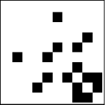
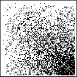
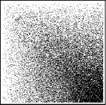
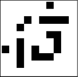
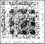
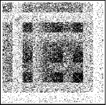
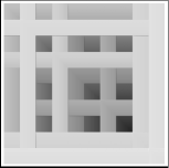
Figure 8: For graph-valued data, the directing random function $F$ in the Aldous-Hoover representation can be regarded as a limit of adjacency matrices: The adjacency matrix of a graph of size $n$ can be represented as a function on $[0,1]^{2}$ by dividing the square into $n\times n$ patches of equal size. On each patch, the representing function is constant, with value equal to the corresponding entry of the adjacency matrix. (In the figure, a black patch indicates a value of one and hence the presence of an edge.) As the size of the graph increases, the subdivision becomes finer, and converges to the function depicted on the right for $n\to\infty$. Convergence is illustrated here for the two functions from Fig. 5. Since the functions are equivalent, the two random graphs within each column are equal in distribution.

Convergence results in statistics study the behavior of the empirical distribution (II.5). The corresponding object for exchangeable graphs is an empirical estimate of the graphon, which is a “checkerboard function”: Given a finite graph $g_{n}$ with $n$ vertices, we subdivide $[0,1]^{2}$ into ${n\times n}$ square patches, resembling the ${n\times n}$ adjacency matrix. We then define a function $w_{g_{n}}$ with constant value 0 or 1 on each patch, equal to the corresponding entry of the adjacency matrix. We call $w_{g_{n}}$ the empirical graphon of $g_{n}$. Examples are plotted in Fig. 8. Since $w_{g_{n}}$ is a valid graphon, it parametrizes an infinite random graph, even though $n$ is finite. Aldous-Hoover theory provides a graph counterpart to the law of large numbers:

Theorem V.1 (Kallenberg [37]).

Let $w$ be a graphon. Suppose we sample a random graph from $w$ one vertex at a time, and $G_{n}$ is the graph given by the first $n$ vertices. Then the distributions defined by $w_{G_{n}}$ converge weakly to the distribution defined by $w$ with probability 1.

A recent development in combinatorics and graph theory is the theory of graph limits [48, 49]. This theory defines a distance measure $\delta_{{}_{\square}}$ on graphons (more details below). The metric can be applied to finite graphs, since the graphs can be represented by the empirical graphon. It is then possible to study conditions under which sequences of graphs converge to a limit. It turns out that limits of graphs can be represented by graphons, and the convergence of graphs corresponds precisely to the weak convergence of the distributions defined by the empirical graphons. This theory refines the Aldous-Hoover theory with a large toolbox of powerful results. We describe a few aspects in the following. The authoritative (and very well-written) reference is [47].

V-A Metric definition of convergence

The most convenient way to define convergence is by defining a metric: If $d$ is a distance measure, we can define $w$ as the limit of $w_{g_{n}}$ if $d(w,w_{g_{n}})\to 0$ as $n\to\infty$. The metric on functions which has emerged as the “right” choice for graph convergence is called the cut metric, and is defined as follows: We first define a norm as

$$\|w\|_{{}_{\square}}:=\sup_{S,T\subset[0,1]}\int_{S\times T}w(x,y)\,\mathrm{d}x\,\mathrm{d}y\,.$$ (V.1)

(The integral is with respect to Lebesgue measure $\mathrm{d}x$ because the variables $U_{i}$ are uniformly distributed.) Intuitively—if we assume for the moment that $w$ can indeed be thought of as a limiting adjacency matrix—$S$ and $T$ are subsets of nodes. The integral (V.1) measures the total number of edges between $S$ and $T$ in the “graph” $w$. Since a partition of the vertices of a graph into two sets is called a cut, $\|\,.\,\|_{{}_{\square}}$ is called the cut norm. The distance measure defined by $d_{{}_{\square}}(w,w^{\prime}):=\|w-w^{\prime}\|_{{}_{\square}}$ is called the cut distance.

Suppose $w$ and $w^{\prime}$ are two distinct functions which parametrize the same distribution on graphs. The distance $d_{{}_{\square}}$ in general perceives such functions as different: The functions in Fig. 8, for instance, define the same graph, but have non-zero distance under $d_{{}_{\square}}$. Hence, if we were to use $d_{{}_{\square}}$ to define convergence, the two sequences of graphs in the figure would converge to two different limits. We therefore modify $d_{{}_{\square}}$ as follows: For any given $w$, let $[w]$ be the set of all functions $w^{\prime}$ which define the same random graph.

$$\delta_{{}_{\square}}(w_{1},w_{2}):=\inf_{w^{\prime}\in[w_{2}]}d_{{}_{\square}}(w_{1},w^{\prime})\;.$$ (V.2)

Informally, we can think of the functions in $[w_{2}]$ as functions obtained from $w_{2}$ by a “rearrangement” like the one illustrated in Fig. 5. The definition above says that, before we measure the distance between $w_{1}$ and $w_{2}$ using $d_{{}_{\square}}$, we rearrange $w_{2}$ in the way that aligns it most closely with $w_{1}$. In Fig. 5, this closest rearrangement would simply reverse the permutation of blocks, so that the two functions would look identical.

The function $\delta_{{}_{\square}}$ is called the cut pseudometric: It is not an actual metric, since it can take value 0 for two distinct functions. It does, however, have all other properties of a metric. By definition, $\delta_{{}_{\square}}(w,w^{\prime})=0$ holds if and only if $w$ and $w^{\prime}$ parametrize the same random graph.

Definition V.2.

We say that a sequence $(g_{n})_{n\in\mathbb{N}}$ of graphs converges if $\delta_{{}_{\square}}(w_{g_{n}},w)\to 0$ for some measurable function ${w:[0,1]^{2}\to[0,1]}$. The function $w$ is called the limit of $(g_{n})$, and often referred to as a graph limit.

Clearly, the graph limit is a graphon, and the two terms are used interchangeably. This definition indeed provides a metric counterpart to convergence of exchangeable graph distributions:

Theorem V.3.

A function $w$ is the graph limit of a sequence $(g_{n})_{n\in\mathbb{N}}$ of graphs if and only if the random graph distributions defined by the empirical graphons $w_{g_{n}}$ converge weakly to the distribution defined by $w$.

V-B Unique parametrization in the Aldous-Hoover theorem

Recall that two graphons can be equivalent, in the sense that they are distinct functions but define the same random graph (they are weakly isomorphic in the language of Section III-D). The equivalence classes $[w]$ form a partition of the space $\mathbf{W}$ of all graphons, which motivates the definition of a “quotient space”: We can define a new space $\widehat{\mathbf{W}}$ by collapsing each equivalence class to a single point. Each element ${\widehat{w}\in\widehat{\mathbf{W}}}$ corresponds to all functions in one equivalence class, and hence to one specific random graph distribution. Since the pseudometric $\delta_{{}_{\square}}$ only assigns distance 0 to two distinct functions if they are equivalent, it turns into a metric on $\widehat{\mathbf{W}}$, and $(\widehat{\mathbf{W}},\delta_{{}_{\square}})$ is a metric space. Although the elements of this space are abstract objects, not actual functions, the space has remarkable analytical properties, and is one of the central objects of graph limit theory.

Since $\widehat{\mathbf{W}}$ contains precisely one element for each ergodic distribution on exchangeable graphs, we can obtain a unique parametrization of exchangeable graph models by using ${\mathbf{T}:=\widehat{\mathbf{W}}}$ as a parameter space: If ${w\in\mathbf{W}}$ is a graphon and $\widehat{w}$ the corresponding element of $\widehat{\mathbf{W}}$—the element to which $w$ was collapsed in the definition of $\widehat{\mathbf{W}}$—we define a family ${\{\mathbf{p}_{\widehat{w}}:\widehat{w}\in\widehat{\mathbf{W}}\}}$ of distributions on exchangeable arrays by taking $\mathbf{p}_{\widehat{w}}$ to be the distribution induced by the uniform sampling scheme described by Eq. III.8 when $W=w$.

Although the existence of such a probability kernel is not a trivial fact, it follows from a technical result of Orbanz and Szegedy [52]. In particular, the Aldous-Hoover theorem for an exchangeable random graph $G$ can then be written as a unique integral decomposition

$$\mathbb{P}(G\in\,.\,)=\int_{\widehat{\mathbf{W}}}{\mathbf{p}_{\widehat{w}}(\,.\,)}\,\nu(\mathrm{d}\widehat{w})\;,$$ (V.3)

in analogy to the de Finetti representation.

V-C Regularity and Concentration

All convergence results we have seen so far provide only asymptotic guarantees of convergence, but no convergence rates. We give two examples of concentration results from graph limit theory, which address similar questions as those asked in mathematical statistics and empirical process theory: How large a graph do we have to observe to obtain reliable estimates?

Underlying these ideas is one of the deepest results of modern graph theory, Szemeredi’s regularity lemma: For every very large graph $g$, there is a small, weighted graph $\hat{g}$ that summarizes all essential structure in $g$. The only condition is that $g$ is sufficiently large. In principle, this means that $\hat{g}$ can be used as an approximation or summary of $g$, but unfortunately, the result is only valid for graphs which are much larger than possible in most conceivable applications. There are, however, weaker forms of this result which hold for much smaller graphs.

To define $\hat{g}$ for a given graph $g$, we proceed as follows: Suppose $\Pi:=\{V_{1},\dotsc,V_{k}\}$ is a partition of $\mathbf{V}(g)$ into $k$ sets. For any two sets $V_{i}$ and $V_{j}$, we define $p_{ij}$ as the probability that two vertices $v\in V_{i}$ and $v^{\prime}\in V_{j}$, each chosen uniformly at random from its set, are connected by an edge. That is,

$$p_{ij}:=\frac{\#\text{ edges between }V_{i},V_{j}}{|V_{i}|\cdot|V_{j}|}\;.$$ (V.4)

The graph $\hat{g}_{\Pi}$ is now defined as the weighted graph with vertex set $\{1,\dotsc,k\}$ and edge weights $p_{ij}$ for edge $(i,j)$. To compare this graph to $g$, it can be helpful to blow it up to a graph $g_{\Pi}$ of the same size as $g$, constructed as follows:

• Each node $i$ is replaced by a clique of size $|V_{i}|$ (with all edges weighted by 1).

• For each pair $V_{i}$ and $V_{j}$, all possible edges between the sets are inserted and weighted by $p_{ij}$.

If we measure how much two graphs differ in terms of the cut distance, $g$ can be approximated by $g_{\Pi}$ as follows:

Theorem V.4 (Weak regularity lemma [29]).

Let $k\in\mathbb{N}$ and let $g$ be any graph. There is a partition $\Pi$ of $\mathbf{V}(g)$ into $k$ sets such that $d_{{}_{\square}}(g,g_{\Pi})\leq 2(\sqrt{\log(k)})^{-1}$.

This form of the result is called “weak” since it uses a less restrictive definition of what it means for $g$ and $g_{\Pi}$ to be close then Szemerédi’s original result. The weaker hypothesis makes the theorem applicable to graphs that are, by the standards of combinatorics, of modest size.

A prototypical concentration result based on Theorem V.4 is the following:

Theorem V.5 ([46, Theorem 8.2]).

Let $f$ be a real-valued function on graphs, which is smooth in the sense that ${|f(g)-f(g^{\prime})|\leq d_{{}_{\square}}(g,g^{\prime})}$ for any two graphs $g$ and $g^{\prime}$ defined on the same vertex set. Let $G(k,g)$ be a random graph of size $k$ sampled uniformly from $g$. Then the distribution of $f(G(k,g))$ concentrates around some value $f_{0}\in\mathbb{R}$, in the sense that

$$\mathbb{P}\Bigl{\{}|f(G(k,g))-f_{0}|>\frac{20}{\sqrt{k}}\Bigr{\}}<2^{-k}\;.$$ (V.5)

The relevance of such results to statistics becomes evident if we think of $f$ as a statistic of a graph or network (such as the edge density) which we try to estimate from an observed subgraph of size $k$. Results of this type, for graphs and other random structures, are collectively known under the term property testing, and are covered by a sizeable literature in combinatorics and theoretical compute science [7, 47].

VI Exchangeability and higher-dimensional arrays

The theory of exchangeable arrays extends beyond 2-dimensional arrays, and, indeed, some of the more exciting implications and applications of the theory rely on the general results. In this section we begin by defining the natural extension of (joint) exchangeability to higher dimensions, and then give higher-dimensional analogues of the theorems of Aldous and Hoover, due to Kallenberg. These theorems introduce exponentially-many additional random variables as the dimension increases, but only a linear number are necessary to produce an arbitrarily good approximation. The presentation owes much to Kallenberg [37].

Definition VI.1 (jointly exchangeable $d$-arrays).

Let $(X_{k_{1},\dotsc,k_{d}})$ be a $d$-dimensional array (or simply $d$-array) of random variables in $\mathbf{X}$. We say that $X$ is jointly exchangeable when

$$(X_{k_{1},\dotsc,k_{d}})\overset{\mbox{\tiny d}}{=}(X_{\pi(k_{1}),\dotsc,\pi(k_{d})})$$ (VI.1)

for every permutation $\pi$ of $\mathbb{N}$.

As in the 2-dimensional representation result, a key ingredient in the characterization of higher-dimensional jointly exchangeable $d$-arrays will be an indexed collection $U$ of i.i.d. latent random variables. In order to define the index set for $U$, let $\tilde{\mathbb{N}}^{d}$ be the space of multisets $J\subseteq\mathbb{N}$ of cardinality $|J|\leq d$. E.g., $\{\!\{1,1,3\}\!\}\in\tilde{\mathbb{N}}^{3}\subseteq\tilde{\mathbb{N}}^{4}$. Rather than two collections—a sequence $(U_{i})$ indexed by $\mathbb{N}$, and a triangular array $(U_{\{\!\{i,j\}\!\}})$ indexed by multisets of cardinality 2—we will use a single i.i.d. collection $U$ indexed by elements of $\tilde{\mathbb{N}}^{d}$. For every $I\subseteq[d]:=\{1,\dotsc,d\}$, we will write $\tilde{k}_{I}$ for the multiset

$$\{\!\{k_{i}:i\in I\}\!\}$$ (VI.2)

and write

$$(U_{\tilde{k}_{I}};\ I\in 2^{[d]}\setminus\emptyset)$$ (VI.3)

for the element of the function space $[0,1]^{2^{[d]}\setminus\emptyset}$ that maps each nonempty subset $I\subseteq[d]$ to the real $U_{\tilde{k}_{I}}$, i.e., the element in the collection $U$ indexed by the multiset $\tilde{k}_{I}\in\tilde{\mathbb{N}}^{|I|}\subseteq\tilde{\mathbb{N}}^{d}$.

Theorem VI.2 (Aldous, Hoover).

Let $U$ be an i.i.d. collection of uniform random variables indexed by multisets $\tilde{\mathbb{N}}^{d}$. A random $d$-array $X:=(X_{k};\ k\in\mathbb{N}^{d})$ is jointly exchangeable if and only if there is random measurable function $F:[0,1]^{2^{[d]}\setminus\emptyset}\to\mathbf{X}$ such that

$$(X_{k};\ k\in\mathbb{N}^{d})\overset{\mbox{\tiny d}}{=}(F(U_{\tilde{k}_{I}};\ I\in 2^{[d]}\setminus\emptyset);\ k\in\mathbb{N}^{d}).$$ (VI.4)

When $d=2$, we recover Theorem III.2 characterizing two-dimensional exchangeable arrays. Indeed, if we write $U_{i}:=U_{\{\!\{i\}\!\}}$ and $U_{ij}:=U_{\{\!\{i,j\}\!\}}$ for notational convenience, then the right hand side of Eq. VI.4 reduces to

$$(F(U_{i},U_{j},U_{ij});\ i,j\in\mathbb{N})$$ (VI.5)

for some random $F:[0,1]^{3}\to\mathbf{X}$. When $d=3$, we instead have

$$(F(U_{i},U_{j},U_{k},U_{ij},U_{ik},U_{jk},U_{ijk});\ i,j,k\in\mathbb{N})$$ (VI.6)

for some random $F:[0,1]^{7}\to\mathbf{X}$, where we have additionally taken $U_{ijk}:=U_{\{\!\{i,j,k\}\!\}}$ for notational convenience.

VI-A Separately exchangeable $d$-arrays

As in the two-dimensional case, arrays with certain additional symmetries can be treated as special cases. In this section, we consider separate exchangeability in the setting of $d$-arrays, and in the next section we consider further generalizations. We begin by defining:

Definition VI.3 (separately exchangeable $d$-arrays).

We say that $d$-array $X$ is separately exchangeable when

$$(X_{k_{1},\dotsc,k_{d}})\overset{\mbox{\tiny d}}{=}(X_{\pi_{1}(k_{1}),\dotsc,\pi_{d}(k_{d})})$$ (VI.7)

for every collection $\pi_{1},\dotsc,\pi_{d}$ of permutations of $\mathbb{N}$.

For every $J\subseteq[d]$, let $1_{J}$ denote its indicator function (i.e., $1_{J}(x)=1$ when $x\in J$ and $0$ otherwise), and let the vector $k_{J}\in\mathbb{Z}_{+}^{d}:=\{0,1,2,\dotsc\}^{d}$ be given by

$$k_{J}:=(k_{1}\,1_{J}(1),\dotsc,k_{d}\,1_{J}(d)).$$ (VI.8)

In order to represent separately exchangeable $d$-arrays, we will use a collection $U$ of i.i.d. uniform random variables indexed by vectors $\mathbb{Z}_{+}^{d}$. Similarly to above, we will write

$$(U_{k_{I}};\ I\in 2^{[d]}\setminus\emptyset)$$ (VI.9)

for the element of the function space $[0,1]^{2^{[d]}\setminus\emptyset}$ that maps each nonempty subset $I\subseteq[d]$ to the real $U_{k_{I}}$, i.e., the element in the collection $U$ indexed by the vector $k_{I}$. Then we have:

Corollary VI.4.

Let $U$ be an i.i.d. collection of uniform random variables indexed by vectors $\mathbb{Z}_{+}^{d}$. A random $d$-array $X:=(X_{k};\ k\in\mathbb{N}^{d})$ is separately exchangeable if and only if there is random measurable function $F:[0,1]^{2^{[d]}\setminus\emptyset}\to\mathbf{X}$ such that

$$(X_{k};\ k\in\mathbb{N}^{d})\overset{\mbox{\tiny d}}{=}(F(U_{k_{I}};\ I\in 2^{[d]}\setminus\emptyset);\ k\in\mathbb{N}^{d}).$$ (VI.10)

We can consider the special cases of $d=2$ and $d=3$ arrays. Then we have, respectively,

$$(F(U_{i0},U_{0j},U_{ij});\ i,j\in\mathbb{N})$$ (VI.11)

for some random $F:[0,1]^{3}\to\mathbf{X}$; and

$$(F(U_{i00},U_{0j0},U_{00k},U_{ij0},U_{i0k},U_{0jk},U_{ijk});\ i,j,k\in\mathbb{N})$$ (VI.12)

for some random $F:[0,1]^{7}\to\mathbf{X}$. As we can see, jointly exchangeable arrays, which are required to satisfy fewer symmetries than their separately exchangeable counterparts, may take $U_{ij0}=U_{0ij}=U_{i0j}=U_{ji0}=\dotsc$. Indeed, one can show that these additional assumptions make jointly exchangeable arrays a strict superset of separately exchangeable arrays, for $d\geq 2$.

VI-B Further generalizations

In applications, it is common for the distribution of an array to be invariant to permutations that act simultaneously on some but not all of the dimensions. E.g., if the first two dimensions of an array index into the same collection of users, and the users are a priori exchangeable, then a sensible notion of exchangeability for the array would be one for which these first two dimensions could be permuted jointly together, but separately from the remaining dimensions.

More generally, we consider arrays that, given a partition of the dimensions of an array into classes, are invariant to permutations that act jointly within each class and separately across classes. More carefully:

Definition VI.5 ($\pi$-exchangeable $d$-arrays).

Let $\pi=\{I_{1},\dotsc,I_{m}\}$ be a partition of $[d]$ into disjoint classes, and let $p=(p^{I};\ I\in\pi)$ be a collection of permutations of $\mathbb{N}$, indexed by the classes in $\pi$. We say that a $d$-array $X$ is $\pi$-exchangeable when

$$(X_{k_{1},\dotsc,k_{d}};\ k\in\mathbb{N}^{d})\overset{\mbox{\tiny d}}{=}(X_{p^{\pi_{1}}(k_{1}),\dotsc,p^{\pi_{d}}(k_{d})};\ k\in\mathbb{N}^{d}),$$ (VI.13)

for every collection $p$ of permutations, where $\pi_{i}$ denotes the subset $I\in\pi$ containing $i$.

We may now cast both jointly and separately exchangeable arrays as $\pi$-exchangeable arrays for particular choices of partitions $\pi$. In particular, when $\pi=\{[d]\}$ we recover joint exchangeability, and when $\pi=\{\{1\},\dotsc,\{d\}\}$, we recover separate exchangeability. Just as we characterized jointly and separately exchangeable arrays, we can characterize $\pi$-exchangeable arrays.

Let $\pi$ be a partition of $[d]$. In order to describe the representation of $\pi$-exchangeable $d$-arrays, we will again need a collection $U$ of i.i.d. uniform random variables, although the index set is more complicated than before: Let $\mathcal{V}(\pi):={\mathsf{X}}_{I\in\pi}\tilde{\mathbb{N}}^{|I|}$ denote the space of functions taking classes $I\in\pi$ to multisets $J\subseteq\mathbb{N}$ of cardinality $J\leq|I|$. We will then take $U$ to be a collection of i.i.d. uniform random variables indexed by elements in $\mathcal{V}(\pi)$.

When $\pi=\{[d]\}$, $\mathcal{V}(\pi)$ is equivalent to the space $\tilde{\mathbb{N}}^{d}$ of multisets of cardinality no more than $d$, in agreement with the index set in the jointly exchangeable case. The separately exchangeable case is also instructive: there $\pi=\{\{1\},\dotsc,\{d\}\}$ and so $\mathcal{V}(\pi)$ is equivalent to the space of functions from $[d]$ to $\tilde{\mathbb{N}}^{1}$, which may again be seen to be equivalent to the space $\mathbb{Z}_{+}^{d}$ of vectors, where $0$ encodes the empty set $\emptyset\in\tilde{\mathbb{N}}^{1}\cap\tilde{\mathbb{N}}^{0}$. For a general partition $\pi$ of $[d]$, an element in $\mathcal{V}(\pi)$ is a type of generalized vector, where, for each class $I\in\pi$ of dimensions that are jointly exchangeable, we are given a multiset of indices.

For every $I\subseteq[d]$, let $\tilde{k}_{\pi I}\in\mathcal{V}(\pi)$ be given by

$$\tilde{k}_{\pi I}(J)=\tilde{k}_{I\cap J},\quad J\in\pi,$$ (VI.14)

where $\tilde{k}_{J}$ is defined as above for jointly exchangeable arrays. We will write

$$(U_{\tilde{k}_{\pi I}};\ I\in 2^{[d]}\setminus\emptyset)$$ (VI.15)

for the element of the function space $[0,1]^{2^{[d]}\setminus\emptyset}$ that maps each nonempty subset $I\subseteq[d]$ to the real $U_{\tilde{k}_{\pi I}}$, i.e., the element in the collection $U$ indexed by the generalized vector $\tilde{k}_{\pi I}$. Then we have:

Corollary VI.6 (Kallenberg [37]).

Let $\pi$ be a partition of $[d]$, and let $U$ be an i.i.d. collection of uniform random variables indexed by generalized vectors $\mathcal{V}(\pi)$. A random $d$-array $X:=(X_{k};\ k\in\mathbb{N}^{d})$ is $\pi$-exchangeable if and only if there is random measurable function $F:[0,1]^{2^{[d]}\setminus\emptyset}\to\mathbf{X}$ such that

$$(X_{k};\ k\in\mathbb{N}^{d})\overset{\mbox{\tiny d}}{=}(F(U_{\tilde{k}_{\pi I}};\ I\in 2^{[d]}\setminus\emptyset);\ k\in\mathbb{N}^{d}).$$ (VI.16)

VI-C Approximations by simple arrays

These representational results require a number of latent random variables exponential in the dimension of the array, i.e., roughly twice as many latent variables are needed as the entries generated in some subarray. Even if a $d$-array is sparsely observed, each observation requires the introduction of potentially $2^{d}$ variables. (In a densely observed array, there will be overlap, and most latent variables will be reused.)

Regardless of whether this blowup poses a problem for a particular application, it is interesting to note that exchangeable $d$-arrays can be approximated by arrays with much simpler structure, known as simple arrays.

Definition VI.7 (simple $d$-arrays).

Let $U=(U^{I}_{k};\ I\in\pi,k\in\mathbb{N})$ be an i.i.d. collection of uniform random variables. We say that a $\pi$-exchangeable $d$-array $X$ is simple when there is a random function $F\colon[0,1]^{[d]}\to\mathbf{X}$ such that

$$(X_{k};\ k\in\mathbb{N}^{d})\overset{\mbox{\tiny d}}{=}(F(U^{\pi_{1}}_{k_{1}},\dots,U^{\pi_{d}}_{k_{d}});\ k\in\mathbb{N}^{d}),$$ (VI.17)

where $\pi_{j}$ is defined as above.

Again, it is instructive to study special cases: in the jointly exchangeable case, taking $U_{j}:=U^{\{[d]\}}_{j}$, we get

$$(F(U_{k_{1}},\dotsc,U_{k_{d}});k\in\mathbb{N}^{d})$$ (VI.18)

and, in the separately exchangeable case, we get

$$(F(U^{1}_{k_{1}},\dotsc,U^{d}_{k_{d}});\ k\in\mathbb{N}^{d}),$$ (VI.19)

taking $U^{i}_{j}:=U^{\{i\}}_{j}$. We may now state the relationship between general arrays and simple arrays:

Theorem VI.8 (simple approximations, Kallenberg [37, Thm. 2]).

Let $X$ be a $\pi$-exchangeable $d$-array. Then there exists a sequence of simple $\pi$-exchangeable arrays $X^{1},X^{2},\dotsc$ such that, for all finite sub-arrays $X_{J}:=(X_{k};k\in J)$, $J\subseteq\mathbb{N}^{d}$, the distributions of $X_{J}$ and $X^{n}_{J}$ are mutually absolutely continuous, and the associated densities tend uniformly to $1$ as $n\to\infty$ for fixed $J$.

VII Sparse random structures and networks

Exchangeable random structures are not “sparse”. In an exchangeable infinite graph, for example, the expected number of edges attached to each node is either infinite or zero. In contrast, graphs representing network data typically have a finite number of edges per vertex, and exhibit properties like power-laws and “small-world phenomena”, which can only occur in sparse graphs. Hence, even though exchangeable graph models are widely used in network analysis, they are inherently misspecified. Since the lack of sparseness is a direct mathematical consequence of exchangeability, networks and sparse random structures pose a problem that seems to require genuinely non-exchangeable models. The development of a coherent theory is, despite intense efforts in mathematics, a largely unsolved problem. In this section, we make the problem more precise and describe how, at least in principle, exchangeability might be substituted by other symmetry properties. The topic raises a host of challenging questions to which, in most cases, we have no answers.

VII-A Dense vs Sparse Random Structures

In an exchangeable structure, events either never occur, or they occur infinitely often with a fixed (though unknown) probability. The simplest example is an exchangeable binary sequence: By de Finetti’s theorem, the binary variables are conditionally i.i.d. with a Bernoulli distribution. If we sample infinitely often, conditionally on the random Bernoulli parameter taking value ${p\in[0,1]}$, the fraction of ones in the sequence will be precisely $p$. Therefore, we either observe a constant proportion of ones (if ${p>0}$) or no ones at all (if ${p=0}$).

In an exchangeable graph, rather than ones and zeros, we have to consider the possible subgraphs (single edges, triangles, five-stars, etc). Each possible subgraph occurs either never, or infinitely often. Since an infinite graph may have infinitely many edges even if it is sparsely connected, the number of edges is best quantified in terms of a rate:

Definition VII.1.

Let $(g_{n})$ be a sequence of graphs ${g_{n}=(v_{n},e_{n})}$, where $g_{n}$ has $n$ vertices. We say that the sequence is sparse if, as $n$ increases, $|e_{n}|$ is of size $O(n)$ (is upper-bounded by $c\cdot n$ for a constant $c$). It is called dense if ${|e_{n}|=\Omega(n^{2})}$ (lower-bounded by ${c\cdot n^{2}}$ for a constant $c$).

If a random graph is sampled step-wise one vertex at a time, the partial graphs at each step also form a sequence, and we can refer to the random graph as dense or sparse, depending on whether the sequence is dense or sparse. (This definition has to be used with caution, since changing the order in which vertices are generated may affect the rate.) A typical example of dense random graphs are infinite random graphs in which each vertex has infinite degree. Random graphs with bounded degrees are sparse. Many important types of graph and array data are inherently sparse: In a social network with billions of users, individual users do not, on average, have billions of friends.

Fact VII.2.

Exchangeable graphs are not sparse. If a random graph is exchangeable, it is either dense or empty.

The argument is simple: Let $G_{n}$ be an $n$-vertex random undirected graph sampled according to Eq. III.8. The expected proportion of edges in present in $G_{n}$, out of all ${{n\choose 2}=\frac{n(n-2)}{2}}$ possible edges, is independent of $n$ and given by ${\varepsilon:=\frac{1}{2}\int_{[0,1]^{2}}W(x,y)\,\mathrm{d}x\,\mathrm{d}y}$. (The factor $\frac{1}{2}$ occurs since $W$ is symmetric.) If ${\varepsilon=0}$, it follows that $G_{n}$ is empty with probability one and therefore trivially sparse. On the other hand, if ${\varepsilon>0}$, we have ${\varepsilon\cdot{n\choose 2}=\Theta(n^{2})}$ edges in expectation and so, by the law of large numbers, $G_{n}$ is dense with probability one.

Remark VII.3 (Graph limits are dense).

The theory of graph limits described in Section V is closely related to exchangeability, and is inherently a theory of dense graphs: If we construct a sequence of graphs with sparsely growing edge sets, convergence in cut metric is still well-defined, but the limit object is always the empty graphon, i.e., a function on $[0,1]^{2}$ which vanishes almost everywhere.

One possible way to generate sparse graphs is of course to modify the sampling scheme for exchangeable graphs to generate fewer edges.

Example VII.4 (The BJR model [14]).

There is a very simple way to modify the Aldous-Hoover approach into one that generates sparse random graphs: Suppose we sample a finite graph with a fixed number $n$ of vertices. We simply multiply the probability in our usual sampling scheme by $1/n$:

$$X_{ij}\sim\mbox{Bernoulli}\Bigl{(}\frac{1}{n}w(U_{i},U_{j})\Bigr{)}\qquad\text{ for }\qquad i,j\leq n\;.$$

Comparison with our argument why exchangeable graphs are dense immediately shows that a graph sampled this way is sparse. More generally, we can multiply $w$ by some other rate function $\rho_{n}$ (instead of specifically ${\rho_{n}=1/n}$), and ask how this model behaves for ${n\to\infty}$. Statistical properties of this model are studied by Bickel, Chen, and Levina [13], who consider the behavior of moment estimators for the edge density, triangle density and other subgraph densities.

An obvious limitation of the BJR model is that it does not actually attempt to model network structure: It can equivalently be sampled by sampling from a graphon as in (III.8) and then deleting each edge independently at random, with probability $(1-\rho_{n})$. (In the parlance of random graph theory, this is exchangeable sampling followed by i.i.d. bond percolation.) In other words, the BJR model modifies an exchangeable graph to fit a first-order statistic of a network (the number of edges), but it cannot generate typical network structures, such as power laws.

VII-B Beyond exchangeability: Symmetry and ergodic theory

The example of networks and sparse structures shows that there are important random structures which are not exchangeable. This raises the question whether integral decompositions and statistical models, which we have throughout derived from exchangeability, can be obtained in a similar manner for structures that are not exchangeable. In principle, that is possible: Exchangeability is a special case of a probabilistic symmetry. It turns out that integral decompositions can be derived from much more general symmetries than exchangeability.

A probabilistic symmetry is defined by choosing a group $\mathbb{G}$ of transformations ${g:\mathbf{X}_{\infty}\to\mathbf{X}_{\infty}}$. A random structure $X_{\infty}$ is called invariant to $\mathbb{G}$ or $\mathbb{G}$-symmetric ${g(X)\overset{\mbox{\tiny d}}{=}X}$ for all ${g\in\mathbb{G}}$. If so, we also say that the distribution of $X_{\infty}$ is $\mathbb{G}$-invariant. For example, a sequence of random variables is exchangeable if and only if the distribution of the sequence is invariant under the group of permutations of $\mathbb{N}$ acting on the indices of the sequence. Exchangeability of arrays (as in the Aldous-Hoover theorem) corresponds with a subgroup generated by row and column permutations. Invariant measures play a key role in several fields of mathematics, especially ergodic theory.

A very general result, the ergodic decomposition theorem, shows that integral decompositions of the form (II.8) are a general consequence of probabilistic symmetries, rather than specifically of exchangeability. The general theme is that there is some correspondence of the form

$$\text{ invariance property }\longleftrightarrow\text{ integral decomposition }\;.$$

In principle, Bayesian models can be constructed based on any type of symmetry, as long as this symmetry defines a useful set of ergodic distributions. The following statement of the ergodic decomposition theorem glosses over various technical details; for a precise statement, see [39, Theorem A1.4].

Theorem VII.5 (Varadarajan [65]).

Let $\mathbb{G}$ be a “nice” group acting on a space $\mathbf{X}^{\infty}$ of infinite structures. Then there exists a family $\mathcal{E}:={\{\mathbf{p}_{\theta}:\theta\in\mathbf{T}\}}$ of distributions on $\mathbf{X}^{\infty}$ such that, if the distribution of a random structure $X_{\infty}$ is $\mathbb{G}$-invariant, it has a representation of the form

$$\mathbb{P}(X_{\infty}\in\,.\,)=\int_{\mathbf{T}}{\mathbf{p}_{\theta}(\,.\,)}\,\nu(\mathrm{d}\theta)\,$$ (VII.1)

for a unique distribution $\nu$ on $\mathbf{T}$. The distributions $\mathbf{p}_{\theta}\in\mathcal{E}$ are the so-called ergodic distributions associated with $\mathbb{G}$.

Figure 9: If $\mathcal{E}$ is finite, the de Finetti mixture representation Eq. II.3 and the more general representation Eq. VII.1 reduce to a finite convex combination. The points inside the set—i.e., the distributions $P$ with the symmetry property defined by the group $\mathbb{G}$—can be represented as convex combinations $P=\sum_{e_{i}\in\mathcal{E}}\nu_{i}e_{i}$, with coefficients $\nu_{i}\geq 0$ satisfying $\sum_{i}\nu_{i}=1$. When $\mathcal{E}$ is infinite, an integral is substituted for the sum.

We have already encountered the components of (VII.1) in Section II: In Bayesian terms, $\mathbf{p}_{\theta}$ again corresponds to the observation distribution and $\nu$ to the prior. Geometrically, the integral representation Eq. VII.1 can be regarded as convex combination. Fig. 9 illustrates this idea for a toy example with three ergodic measures. A special case of the ergodic decomposition theorem is well-known in Bayesian theory as a result of Freedman [27, 28]:

Example VII.6 (Freedman’s theorem).

Consider a sequence ${X_{1},X_{2},\dotsc}$ as in de Finetti’s theorem. Now replace invariance under permutations by a stronger condition: Let $\mathrm{O}(n)$ be the orthogonal group of rotations and reflections on $\mathbb{R}^{n}$, i.e., the set of ${n\times n}$ orthogonal matrices. We now demand that, if we regard any initial sequence of $n$ variables as a random vector in $\mathbb{R}^{n}$, then rotating and/or reflecting this vector does not change the distribution of the sequence: That is, for every ${n\in\mathbb{N}}$ and ${M\in\mathrm{O}(n)}$,

$$(X_{1},X_{2},\dotsc)\overset{\mbox{\tiny d}}{=}(M(X_{1},\dotsc,X_{n}),X_{n+1},\dotsc)\,.$$ (VII.2)

In the language of Theorem VII.5, the group $G$ is the set of all rotations and reflections acting on all finite prefixes of a sequence. For every $\sigma>0$, let $\mathcal{N}_{\sigma}$ be the distribution of zero-mean Gaussian random variable with standard deviation $\sigma$. Freedman showed that, if $X^{\infty}$ satisfies Eq. VII.2, then its distribution is a scale mixture of Gaussians:

$$\mathbb{P}(X^{\infty}\in\,.\,)=\int_{\mathbb{R}_{+}}{\mathcal{N}^{\infty}_{\sigma}(\,.\,)}\,\nu_{\mathbb{R}_{+}}(\mathrm{d}\sigma)\,.$$ (VII.3)

Thus, $\mathcal{E}$ contains all factorial distributions of zero-mean Gaussian distributions on $\mathbb{R}$, $\mathbf{T}$ is the set $\mathbb{R}_{>0}$ of variances, and $\nu$ a distribution on $\mathbb{R}_{>0}$.

Compared to de Finetti’s theorem, where $\mathbb{G}$ is the group of permutations, Freedman’s theorem increases the size of $\mathbb{G}$: Any permutation can be represented as an orthogonal matrix, but here rotations have been added as well. In other words, we are strengthening the hypothesis by imposing more constraints on the distribution of $X^{\infty}$. As a result, the set $\mathcal{E}$ of ergodic measures shrinks from all factorial measures to the set of factorials of zero-mean Gaussians. This is again an example of a general theme:

$$\text{larger group}\quad\longleftrightarrow\quad\text{more specific representation}$$

In contrast, the Aldous-Hoover theorem weakens the hypothesis of de Finetti’s theorem—in the matrix case, for instance, the set of all permutations of the index set $\mathbb{N}^{2}$ is restricted to those which preserve rows and columns—and hence yields a more general representation.

Remark VII.7 (Symmetry and sufficiency).

An alternative way to define symmetry in statistical models is through sufficient statistics: Intuitively, a symmetry property identifies information which is not relevant to the statistical problem; so does a sufficient statistic. For example, the empirical distribution retains all information about a sample except for the order in which observations were recorded. The empirical distribution is hence a sufficient statistic for the set distributions of exchangeable sequences. In an exchangeable graph model, the empirical graphon (the checkerboard function in Fig. 8) is a sufficient statistic. If the sufficient statistic is finite-dimensional and computes an average $\frac{1}{n}\sum_{i}S_{0}(x_{i})$ over observations for some function $S_{0}$, the ergodic distributions are exponential family models [43]. A readable introduction to this topic is given by Diaconis [20]. The definitive reference is the monograph of Lauritzen [44], who refers to the set $\mathcal{E}$ of ergodic distributions as an extremal family.

Not every probabilistic symmetry is applicable in statistics in the same way as exchangeability is. To be useful to statistics, the symmetry must satisfy two conditions:

1. The set $\mathcal{E}$ of ergodic measures should be a “small” subset of the set of symmetric measures.

2. The measures $\mathbf{p}_{\theta}$ should have a tractable representation, such as Kingman’s paint-box or the Aldous-Hoover sampling scheme.

Theorem VII.5 guarantees neither. If (1) is not satisfied, the representation is useless for statistical purposes: The integral representation Eq. VII.1 means that the information in $X_{\infty}$ is split into two parts, the information contained in the parameter value $\theta$ (which a statistical procedure tries to extract) and the randomness represented by $\mathbf{p}_{\theta}$ (which the statistical procedure discards). If the set $\mathcal{E}$ is too large, $\Theta$ contains almost all the information in $X_{\infty}$, and the decomposition becomes meaningless. We will encounter an appealing notion of symmetry for sparse networks in the next section—which, however, seems to satisfy neither condition (1) or (2). It is not clear at present whether there are useful types of symmetries which do not imply some form of invariance to a group of permutations. Although the question is abstract, the incompatibility of sparseness and exchangeability means it is directly relevant to Bayesian statistics.

VII-C Stationary networks and involution invariance

Is there a form of invariance that yields statistical models for network data? There is indeed a very natural notion of invariance in networks, called involution invariance, which we describe in more detail below. This property has interesting mathematical properties and admits an ergodic decomposition as in Theorem VII.5, but it seems to be too weak for applications in statistics.

A crucial difference between network structures and exchangeable graphs is that, in most networks, location in the graph matters. If conditioning on location is informative, exchangeability is broken. Probabilistically, location is modeled by marking a distinguished vertex in the graph. A rooted graph $(g,v)$ is simply a graph $g$ in which a particular vertex $v$ has been marked. A very natural notion of invariance for networks is called involution invariance [2] or unimodularity [11], and can be thought of as a form of stationarity:

Definition VII.8.

Let $P$ be the distribution of a random rooted graph, and define a distribution $\tilde{P}$ as follows: A sample ${(G,w)\sim\tilde{P}}$ is generated by sampling ${(G,v)\sim P}$, and then sampling $w$ uniformly from the neighbors of $v$ in $G$. The distribution $P$ is called involution invariant if $P=\tilde{P}$.

The definition says that, if an observer randomly walks along the graph $G$ by moving to a uniformly selected neighbor in each step, the distribution of the network around the observer remains unchanged (although the actual neighborhoods in a sampled graph may vary).

Involution invariance is a symmetry property which admits an ergodic decomposition, and Aldous and Lyons [2] have characterized the ergodic measures. This characterization is abstract, however, and there is no known “nice” representation resembling, for example, the sampling scheme for exchangeable graphs. Thus, of the two desiderata described in Section VII-B, property (2) does not seem to hold. We believe that property (1) does not hold either: Although we have no proof at present, it seems that involution invariance is too weak a constraint to yield interesting statistical models (i.e., the set of ergodic distributions is a “large” subset of the involution invariant distributions).

Since exchangeability and involution invariance are the only well-studied probabilistic symmetries for random graphs, the question how statistical models of networks can be characterized is an open problem:

Is there a notion of probabilistic symmetry whose ergodic measures in (VII.1) describe useful statistical models for sparse graphs with network properties?

There is a sizeable literature on sparse random graph models which can model power laws and other network properties; see, for example [23]. These are probability models and can be simulated, but estimation from data is often intractable, due to stochastic dependencies between the edges in the random graph. On the other hand, some dependence between edges is necessary to obtain a power law and similar properties. Hence, a suitable notion of symmetry would have to restrict dependencies between edges sufficiently to permit statistical inference, but not to the full conditional independence characteristic of the exchangeable case.

VIII Further References

Excellent non-technical references on the general theory of exchangeable arrays and other exchangeable random structures are two recent surveys by Aldous [6, 5]. His well-known lecture notes [4] also cover exchangeable arrays. The most comprehensive available reference on the general theory is the monograph by Kallenberg [39] (which presupposes in-depth knowledge of measure-theoretic probability). Kingman’s original article [41] provides a concise reference on exchangeable random partitions. A thorough, more technical treatment of exchangeable partitions can be found in [12].

Schervish [59] gives an insightful discussion of the application of exchangeability to Bayesian statistics. There is a close connection between probabilistic symmetries (such as exchangeability) and sufficient statistics, which is covered by a substantial literature. See Diaconis [20] for an introduction and further references. For applications of exchangeability results to machine learning models, see [26], who discuss applications of the partial exchangeability result of Diaconis and Freedman [21] to the infinite hidden Markov model [10].

The theory of graph limits in its current form was initiated by Lovász and Szegedy [48, 49] and Borgs et al. [15]. It builds on work of Frieze and Kannan [29], who introduced both the weak regularity lemma (Theorem V.4) and the cut norm $d_{{}_{\square}}$. In the framework of this theory, the Aldous-Hoover representation of exchangeable graphs can be derived by purely analytic means [48, Theorem 2.7]. The connection between graph limits and Aldous-Hoover theory was established, independently of each other, by Diaconis and Janson [22] and by Austin [8]. An accessible introduction to the analytic perspective is the survey [46], which assumes basic familiarity with measure-theoretic probability and functional analysis, but is largely non-technical. The monograph [47] gives a comprehensive account.

Historically, the Aldous-Hoover representation was established in independent works of Aldous and of Hoover in the late 1970s. Aldous’ proof used probability-theoretic methods, whereas Hoover, a logician, leveraged techniques from model theory. In 1979, Kingman [42] writes

…a general solution has now been supplied by Dr David Aldous of Cambridge. […] The proof is at present very complicated, but there is reason to hope that the techniques developed can be applied to more general experimental designs.

Aldous’ paper [3], published in 1981, attributes the idea of the published version of the proof to Kingman. The results were later generalized considerably by Kallenberg [37].

Acknowledgments. We have learned much about random graphs from Cameron Freer, and are also indebted to James Robert Lloyd for many useful discussions. Two anonymous reviewers have provided very detailed feedback, which in our opinion has greatly improved the article. We thank Karolina Dziugaite, Creighton Heaukalani, Jonathan Huggins and Christian Steinrücken for helpful comments on the manuscript.

References

- Airoldi et al. [2008] Airoldi, E. M., Blei, D. M., Feinberg, S. E., and Xing, E. P. (2008). Mixed-membership stochastic blockmodels. J. Machine Learn. Res., 9, 1981–2014.
- Aldous and Lyons [2007] Aldous, D. and Lyons, R. (2007). Processes on unimodular random networks. Electron. J. Probab., 12, no. 54, 1454–1508.
- Aldous [1981] Aldous, D. J. (1981). Representations for partially exchangeable arrays of random variables. J. Multivariate Anal., 11(4), 581–598.
- Aldous [1985] Aldous, D. J. (1985). Exchangeability and related topics. In P. L. Hennequin, editor, École d’Été de Probabilités de Saint-Flour XIII - 1983, number 1117 in Lecture Notes in Mathematics, pages 1–198. Springer.
- Aldous [2010a] Aldous, D. J. (2010a). Exchangeability and continuum limits of discrete random structures. In Proceedings of the International Congress of Mathematicians. Volume I, pages 141–153. Hindustan Book Agency, New Delhi.
- Aldous [2010b] Aldous, D. J. (2010b). More uses of exchangeability: representations of complex random structures. In Prob. math. genetics, volume 378 of London Math. Soc. Lecture Note Ser., pages 35–63. Cambridge Univ. Press, Cambridge.
- Alon and Spencer [2008] Alon, N. and Spencer, J. H. (2008). The Probabilistic Method. J. Wiley & Sons.
- Austin [2008] Austin, T. (2008). On exchangeable random variables and the statistics of large graphs and hypergraphs. Probab. Surv., 5, 80–145.
- Bacallado et al. [2013] Bacallado, S., Favaro, S., and Trippa, L. (2013). Bayesian nonparametric analysis of reversible Markov chains. Ann. Statist., 41(2), 870–896.
- Beal et al. [2002] Beal, M. J., Ghahramani, Z., and Rasmussen, C. (2002). The infinite hidden Markov model. In T. G. Dietterich, S. Becker, and Z. Ghrahmani, editors, Adv. Neural Inform. Process. Syst. (NIPS) 14, pages 577–584.
- Benjamini and Schramm [2001] Benjamini, I. and Schramm, O. (2001). Recurrence of distributional limits of finite planar graphs. Electron. J. Probab., 6, no. 23, 13 pp. (electronic).
- Bertoin [2006] Bertoin, J. (2006). Random Fragmentation and Coagulation Processes. Cambridge University Press.
- Bickel et al. [2011] Bickel, P. J., Chen, A., and Levina, E. (2011). The method of moments and degree distributions for network models. Ann. Statist., 39(5), 2280–2301.
- Bollobás et al. [2007] Bollobás, B., Janson, S., and Riordan, O. (2007). The phase transition in inhomogeneous random graphs. Random Struct. Alg., 31(1), 3–122.
- Borgs et al. [2006] Borgs, C., Chayes, J., Lovász, L., Sós, V. T., Szegedy, B., and Vesztergombi, K. (2006). Graph limits and parameter testing. In Proc. 38th Annu. ACM Symp. Theory Comput., pages 261–270.
- Borgs et al. [2010] Borgs, C., Chayes, J., and Lovász, L. (2010). Moments of two-variable functions and the uniqueness of graph limits. Geom. Func. Anal., 19(6), 1597–1619.
- Broderick et al. [2013a] Broderick, T., Jordan, M. I., and Pitman, J. (2013a). Cluster and feature modeling from combinatorial stochastic processes. Statist. Sci., 28(3), 289–312.
- Broderick et al. [2013b] Broderick, T., Pitman, J., and Jordan, M. I. (2013b). Feature allocations, probability functions, and paintboxes. Bayesian Analysis, 8(4), 801––836.
- Bühlmann [1960] Bühlmann, H. (1960). Austauschbare stochastische Variabeln und ihre Grenzwertsätze. Ph.D. thesis, ETH Zürich. University of California Press, 1960.
- Diaconis [1992] Diaconis, P. (1992). Sufficiency as statistical symmetry. In F. Browder, editor, Proc. 100th Ann. Am. Math. Soc., pages 15–26. American Mathematical Society.
- Diaconis and Freedman [1980] Diaconis, P. and Freedman, D. (1980). De Finetti’s theorem for Markov chains. Ann. Probab., 8(1), pp. 115–130.
- Diaconis and Janson [2008] Diaconis, P. and Janson, S. (2008). Graph limits and exchangeable random graphs. Rendiconti di Matematica, Serie VII, 28, 33–61.
- Durrett [2006] Durrett, R. (2006). Random Graph Dynamics. Cambridge University Press.
- de Finetti [1930] de Finetti, B. (1930). Funzione caratteristica di un fenomeno aleatorio. Atti Reale Accademia Nazionale dei Lincei, VI(4), 86–133.
- de Finetti [1937] de Finetti, B. (1937). La prévision: ses lois logiques, ses sources subjectives. Ann. Inst. H. Poincaré, 7(1), 1–68.
- Fortini and Petrone [2012] Fortini, S. and Petrone, S. (2012). Predictive construction of priors in Bayesian nonparametrics. Braz. J. Probab. Stat., 26(4), 423–449.
- Freedman [1962] Freedman, D. A. (1962). Invariants under mixing which generalize de Finetti’s theorem. Ann. Math. Statist., 33, 916–923.
- Freedman [1963] Freedman, D. A. (1963). Invariants under mixing which generalize de Finetti’s theorem. Ann. Math. Statist., 34(1194–1216).
- Frieze and Kannan [1999] Frieze, A. and Kannan, R. (1999). Quick approximation to matrices and applications. Combinatorica, 19(2), 175–220.
- Griffiths and Ghahramani [2006] Griffiths, T. L. and Ghahramani, Z. (2006). Infinite latent feature models and the Indian buffet process. In Adv. Neural Inform. Processing Syst. (NIPS) 18, pages 475–482. MIT Press, Cambridge, MA.
- Hewitt and Savage [1955] Hewitt, E. and Savage, L. J. (1955). Symmetric measures on Cartesian products. Trans. Am. Math. Soc., 80(2), 470–501.
- Hjort et al. [2010] Hjort, N., Holmes, C., Müller, P., and Walker, S., editors (2010). Bayesian Nonparametrics. Cambridge University Press.
- Hoff [2008] Hoff, P. (2008). Modeling homophily and stochastic equivalence in symmetric relational data. In Adv. Neural Inf. Process. Syst. (NIPS) 19.
- Hoff [2011] Hoff, P. D. (2011). Separable covariance arrays via the Tucker product, with applications to multivariate relational data. Bayesian Analysis, 6(2), 179–196.
- Holland et al. [1983] Holland, P. W., Laskey, K. B., and Leinhardt, S. (1983). Stochastic blockmodels: First steps. Social Networks, 5(2), 109–137.
- Hoover [1979] Hoover, D. N. (1979). Relations on probability spaces and arrays of random variables. Technical report, Institute of Advanced Study, Princeton.
- Kallenberg [1999] Kallenberg, O. (1999). Multivariate sampling and the estimation problem for exchangeable arrays. J. Theoret. Probab., 12(3), 859–883.
- Kallenberg [2001] Kallenberg, O. (2001). Foundations of Modern Probability. Springer, 2nd edition.
- Kallenberg [2005] Kallenberg, O. (2005). Probabilistic Symmetries and Invariance Principles. Springer.
- Kemp et al. [2006] Kemp, C., Tenenbaum, J., Griffiths, T., Yamada, T., and Ueda, N. (2006). Learning systems of concepts with an infinite relational model. In Proc. Nat. Conf. A.I. (IJCAI), volume 21, pages 381–389.
- Kingman [1978] Kingman, J. F. C. (1978). The representation of partition structures. J. London Math. Soc., 2(18), 374–380.
- Kingman [1979] Kingman, J. F. C. (1979). Discussion of: “On the Reconciliation of Probability Assessments” by D. V. Lindley, A. Tversky and R. V. Brown. J. Roy. Statist. Soc. Ser. A, 142(2), 171.
- Küchler and Lauritzen [1989] Küchler, U. and Lauritzen, S. L. (1989). Exponential families, extreme point models and minimal space-time invariant functions for stochastic processes with stationary and independent increments. Scand. J. Stat., 16, 237–261.
- Lauritzen [1988] Lauritzen, S. L. (1988). Extremal Families and Systems of Sufficient Statistics. Lecture Notes in Statistics. Springer.
- Lloyd et al. [2012] Lloyd, J. R., Orbanz, P., Roy, D. M., and Ghahramani, Z. (2012). Random function priors for exchangeable arrays. In Adv. Neural Inform. Processing Syst. (NIPS) 25, pages 1007–1015.
- Lovász [2009] Lovász, L. (2009). Very large graphs. In D. Jerison, B. Mazur, T. Mrowka, W. Schmid, R. Stanley, and S. T. Yau, editors, Current Developments in Mathematics, pages 67–128. International Press.
- Lovász [2013] Lovász, L. (2013). Large Networks and Graph Limits. American Mathematical Society.
- Lovász and Szegedy [2006] Lovász, L. and Szegedy, B. (2006). Limits of dense graph sequences. J. Combin. Theory Ser. B, 96, 933–957.
- Lovász and Szegedy [2007] Lovász, L. and Szegedy, B. (2007). Szemerédi’s lemma for the analyst. Geom. Func. Anal., 17(1), 252–270.
- MacEachern [2000] MacEachern, S. N. (2000). Dependent Dirichlet processes. Technical report, Ohio State University.
- Miller et al. [2009] Miller, K. T., Griffiths, T. L., and Jordan, M. I. (2009). Nonparametric latent feature models for link prediction. In Adv. Neural Inform. Process. Syst. (NIPS) 20, pages 1276–1284.
- Orbanz and Szegedy [2013] Orbanz, P. and Szegedy, B. (2013). Borel liftings of graph limits. http://arxiv.org/abs/1312.7351v1.
- Paisley et al. [2010] Paisley, J., Zaas, A., Woods, C., Ginsburg, G., and Carin, L. (2010). A stick-breaking construction of the beta process. In Proc. Int. Conf. Machine Learning (ICML), pages 847–854.
- Paisley et al. [2012] Paisley, J., Blei, D., and Jordan, M. (2012). Stick-breaking beta processes and the Poisson process. In Proc. Int. Conf. A.I. Stat. (AISTATS).
- Pitman [2006] Pitman, J. (2006). Combinatorial stochastic processes, volume 1875 of Lecture Notes in Mathematics. Springer-Verlag, Berlin. Lectures from the 32nd Summer School on Probability Theory held in Saint-Flour, July 7–24, 2002, With a foreword by Jean Picard.
- Rasmussen and Williams [2006] Rasmussen, C. E. and Williams, C. K. I. (2006). Gaussian Processes for Machine Learning. The MIT Press.
- Roy [2011] Roy, D. M. (2011). Computability, inference and modeling in probabilistic programming. Ph.D. thesis, Massachusetts Institute of Technology.
- Roy and Teh [2009] Roy, D. M. and Teh, Y. W. (2009). The Mondrian process. In Adv. Neural Inform. Processing Syst. (NIPS) 21, pages 1377–1384.
- Schervish [1995] Schervish, M. J. (1995). Theory of Statistics. Springer.
- Sethuraman [1994] Sethuraman, J. (1994). A constructive definition of Dirichlet priors. Statist. Sinica, 4(2), 639–650.
- Teh and Jordan [2010] Teh, Y. W. and Jordan, M. I. (2010). Hierarchical Bayesian nonparametric models with applications. In N. L. Hjort, C. Holmes, P. Müller, and S. G. Walker, editors, Bayesian Nonparametrics. Cambridge University Press.
- Teh et al. [2007] Teh, Y. W., Görür, D., and Ghahramani, Z. (2007). Stick-breaking construction for the Indian buffet process. In Proc. 11th Conf. A.I. Stat. (AISTATS), pages 556–563.
- Teh et al. [2011] Teh, Y. W., Blundell, C., and Elliott, L. (2011). Modelling genetic variations using fragmentation-coagulation processes. In Adv. Neural Inf. Process. Syst. (NIPS) 24, pages 819–827.
- Thibaux and Jordan [2007] Thibaux, R. and Jordan, M. I. (2007). Hierarchical beta processes and the Indian buffet process. In Proc. 11th Conf. A.I. Stat. (AISTATS), pages 564–571.
- Varadarajan [1963] Varadarajan, V. S. (1963). Groups of automorphisms of Borel spaces. Trans. Amer. Math. Soc., 109(2), 191–220.
- Wasserman and Anderson [1987] Wasserman, S. and Anderson, C. (1987). Stochastic a posteriori blockmodels: Construction and assessment. Social Networks, 9(1), 1–36.
- Wolfe and Olhede [2013] Wolfe, P. J. and Olhede, S. C. (2013). Nonparametric graphon estimation. http://arxiv.org/abs/1309.5936v1.
- Xu et al. [2006] Xu, Z., Tresp, V., Yu, K., and Kriegel, H.-P. (2006). Infinite hidden relational models. In Proc. 22nd Int. Conf. Uncertainty in Artificial Intelligence (UAI), pages 544–551.
- Xu et al. [2012] Xu, Z., Yan, F., and Qi, Y. (2012). Infinite Tucker Decomposition: Nonparametric Bayesian Models for Multiway Data Analysis. In Proc. 29th Int. Conf. Machine Learning (ICML).
- Zabell [1995] Zabell, S. L. (1995). Characterizing Markov exchangeable sequences. J. Theoret. Probab., 8(1), 175–178.