On How the Scalar Propagator Transforms Covariantly in Spinless Quantum Electrodynamics

Abstract

Gauge covariance properties of the scalar propagator in spinless/scalar quantum electrodynamics (SQED) are explored in the light of the corresponding Landau-Khalatnikov-Fradkin transformation (LKFT). These transformations are non perturbative in nature and describe how each Green function of the gauge theory changes under a variation of the gauge parameter. With a simple strategy, considering the scalar propagator at the tree level in Landau gauge, we derive a non perturbative expression for this propagator in an arbitrary covariant gauge and three as well as four space–time dimensions. Some relevant kinematical limits are discussed. Particularly, we compare our findings in the weak coupling regime with the direct one-loop calculation of the said propagator and observe perfect agreement up to an expected gauge independent term. We further notice that some of the coefficients of the all-order expansion for the propagator are fixed directly from the LKFT, a fact that makes this set of transformations appealing over ordinary perturbative calculations in gauge theories.

I Introduction

Gauge principle has become the foundation of our modern understanding of fundamental interactions among the basic constituents of the Universe. Demanding the invariance of the Lagrangian under local gauge transformations dictates the form of the interactions among quarks and leptons in the celebrated Standard Model of Particle Physics. The only abelian theory based upon the gauge principle is the theory of electromagnetic interactions –a historical account of the origins of gauge invariance can be found in excellent reviews roots –. The topic is so important that it is mandatory in many textbooks at the graduate and advanced undergraduate levels. Classically, Maxwell’s equations which describe electromagnetic interactions are usually solved for the auxiliary scalar and vector potentials $\phi(\mathbf{x},t)$ and $\mathbf{A}(\mathbf{x},t)$ rather than for the electric $\mathbf{E}(\mathbf{x},t)$ and magnetic field $\mathbf{B}(\mathbf{x},t)$ themselves. These fields can later be obtained from the potentials as follows :

$$\mathbf{B}(\mathbf{x},t) = \nabla\times\mathbf{A}(\mathbf{x},t)\;,$$ (1a)

$$\mathbf{E}(\mathbf{x},t) = -\nabla\phi(\mathbf{x},t)-\frac{\partial\mathbf{A}(\mathbf{x},t)}{\partial t}\;,$$ (1b)

in cgs units. The choice of the electromagnetic potentials is not unique, though the fields $\mathbf{E}(\mathbf{x},t)$ and $\mathbf{B}(\mathbf{x},t)$ remain unaltered for every possible equivalent configuration of the auxiliary potentials Jackson . At the quantum level, gauge symmetry is often introduced as a set of transformation rules for the elementary fields –which represent particles– of a given theory that generate interaction terms and leave the resulting Lagrangian invariant Holstein ; Noether . Gauge invariance of a field theory is of cardinal importance because it is intimately connected to its renormalizability. Physical observables like the components of the field strength tensor LagrangianGaugeTrans or the $S$-matrix elements OpGauge remain unchanged under gauge transformations. Gauge symmetry is also manifest at the level of field equations. In quantum electrodynamics (QED), for instance, it is by virtue of gauge symmetry that different $(n+1)-$point Green functions are related to $n-$point ones through the so-called Ward-Green-Takahashi identities WGTI . Possibly the best known of these identities relate the 3-point vertex $\Gamma^{\mu}(k,p)$ to the 2-point (inverse) fermion propagator $S_{F}^{-1}(p)$ in the form

$$(k-p)_{\mu}\Gamma^{\mu}(k,p)=S_{F}^{-1}(k)-S_{F}^{-1}(p)\;.$$ (2)

An enlarged set of these identities, referred to as the Nielsen identities Nielsen , have been used to demonstrate that the poles of the propagators on the real time-like axis, corresponding to the physical masses of the particles represented by these fields, are gauge invariant quantities Steele . Furthermore, to prove the renormalizability of a theory (namely, its predictive power), both sets of identities should be valid order by order in perturbation theory. At high energies, like those in which collisions take place in the Large Hadron Collider (LHC) at CERN, the theoretical predictions of Standard Model can be compared with the experiment in a perturbative scheme that allows to formulate a framework to systematically improve the predictions for scattering cross sections, decay widths and other quantities.

There exist a different set of rules which specify the way Green functions change under a gauge transformation. These rules carry the name of Landau-Khalatnikov-Fradkin transformations (LKFTs) LKF and were first introduced in QED. Later on, LKFT’s have been re-discovered in the past decades by several authors LKFnew . In deriving them, no assumption is made on the strength of the interaction, and therefore the transformations are valid both in the strong and weak coupling regimes. This feature is very important for theories of strong-interactions like quantum chromodynamics (QCD) at low energies, that is, in the realm of hadron physics. Understanding the nature of hadron spectra is one of the most challenging problems in particle physics simply because QCD becomes highly non-linear at low energies. Therefore, very specialized techniques, which include lattice simulations lattice , effective theories effective and other approaches like the solution of the field equations of a quantum field theory esd have to be developed in order to gain and understanding of confinement and dynamical chiral symmetry breaking, two emergent phenomena of QCD responsible of the nature of the hadron spectra. For detailed reviews and recent applications of these equations, one can consult the references esd1 .

LKFTs have been employed in this context to enhance validity of the predictions arising from the equations of motion of QED is several space-time dimensions LKFinSDE . On the other hand, these transformations also provide important information about the all order perturbative expansion of the Green functions when some perturbative form of these functions is used as input. In this work we shall exploit the remarkable features of LKFTs to have a glimpse into the non-perturbative structure of the scalar propagator in SQED in 3 and 4 space–time dimensions whose perturbative structure at the one loop level has been studied in detail recently Yajaira . We shall observe that when the input we use in the LKFT approach is the perturbative propagator at a given order $n_{0}$ in perturbation theory in Landau gauge, all the gauge dependent terms at the $(n_{0}+1)$-order get fixed by the weak coupling expansion of its corresponding LKFT. The paper is organized as follows: In the next section we introduce the LKFT for the scalar propagator. We discuss the three dimensional case in various interesting limits in Sect. III. Section IV is devoted to the 4D case, discussed in detail in relevant kinematic limits. For the sake of comparison, we perform an ordinary one-loop calculation of the scalar propagator and contrast the prediction with those coming from the LKFT approach in Sect. V. Our final remarks are presented in Sec. VI, and some calculations are discussed in an appendix. At different stages of the discussion, crucial steps that lead to our results are proposed as exercises for the intrepid reader.

II Gauge Covariance and the Scalar Propagator

Let us begin by recalling the Lagrangian of SQED. In order to keep the notation as clear as possible, we do not consider the space-time dependence of the fields in the following. Free charged scalar particles (with the fundamental charge $e$) of mass $m$, represented by the fields $\phi$ and $\phi^{*}$ are described by the Lagrangian

$${\cal L}_{\rm scalar}=\frac{1}{2}\left[(\partial_{\mu}\phi)(\partial^{\mu}\phi)^{*}\right]-\frac{1}{2}\,m^{2}\,\phi^{*}\phi\;.$$ (3)

Next, we allow these fields to couple electromagnetically with photons. This is achieved by promoting the ordinary derivatives to the covariant ones

$$\partial_{\mu}\to\mathscr{D}_{\mu}=\partial_{\mu}+ieA_{\mu}\;,$$ (4)

where the vector field $A_{\mu}$ represents the electromagnetic potential, which is associated with the photon wavefunction in the quantum theory. We further add the electromagnetic kinetic term (Maxwell term),

$${\cal L}_{\gamma}=-\frac{1}{4}F_{\mu\nu}F^{\mu\nu}\;,$$ (5)

with $F^{\mu\nu}=\partial^{\mu}A^{\nu}-\partial^{\nu}A^{\mu}$ representing the field strength tensor, as usual. Finally, for the consistency of the second quantized theory, we must add two terms. The first additional one is the covariant gauge fixing term, which gets rid of spurious degrees of freedom in a covariant manner, and the second is the scalar self-interaction quartic term, which is required for the renormalizability of the theory. Therefore, we shall be working with the Lagrangian:

$${\cal L}=\frac{1}{2}\left[(\mathscr{D}_{\mu}\phi)(\mathscr{D}^{\mu}\phi)^{*}\right]-\frac{1}{2}\,m^{2}\,\phi^{*}\phi-\frac{1}{4}F_{\mu\nu}F^{\mu\nu}-\frac{1}{2\xi}(\partial_{\mu}A^{\mu})^{2}-\frac{\lambda}{4}\left(\phi^{*}\phi\right)^{2},$$ (6)

where $\lambda$ the coupling for the scalar self-interaction and $\xi$ is the covariant gauge parameter. The above Lagrangian (6) describes, for instance, the electromagnetic and self-interactions of charged scalars like pions at low energies where they can be considered as point particles. Observe that the electromagnetic dynamics between scalar particles is oblivious of the self interaction part other than the technicalities on renormalization. As we are focussing only on the gauge covariance relations, the non-gauge 4-point self interaction is irrelevant to our purpose. Hence, in the remainder of the article, we set $\lambda=0$.

The next step in our program is to identify the most important quantities that are relevant for our discussion, namely, the propagators. The free photon propagator associated to the Lagrangian (6) is

$$\Delta_{\mu\nu}^{(0)}(q;\xi)=-\frac{1}{q^{2}}\left(g_{\mu\nu}-\frac{q_{\mu}q_{\nu}}{q^{2}}\right)+\xi\frac{q_{\mu}q_{\nu}}{q^{4}}\;.$$ (7)

We explicitly label the propagators with the covariant gauge parameter $\xi$ (a real number) as we would be interested in their expression in different gauges. The photon propagator (7) changes from gauge to gauge simply by choosing different values of $\xi$. Some useful gauges are the Feynman gauge ($\xi=1$), amenable for perturbative calculations; the Landau gauge ($\xi=0$), which retains the transverse nature of the photons in a manifestly covariant form; or Yennie gauge ($\xi=3$), where the mass shell renormalization scheme can be implemented without introducing spurious infrared divergences. The tree level scalar propagator, in a $d$-dimensional Minkowski space-time, has the form

$$iD^{(0)}_{d}(p;\xi)=\frac{i}{p^{2}-m^{2}},$$ (8)

where the Feynman prescription $+i\varepsilon$ is understood, but omitted. As stated by the gauge principle, a change in the photon propagator (7) should be compensated by a change in the scalar propagator (8) to retain the gauge invariance of the Lagrangian. There exist a set of transformation rules that specify the explicit form in which all the Green functions in our theory change under local gauge transformations. These are called Landau-Khalatnikov-Fradkin transformations (LKFT) LKF and have been discovered and re-discovered during the past 60 years LKFnew . These transformations have the simplest structure in Euclidean coordinate space. Therefore, we relate the propagator in $d$-dimensional Euclidean coordinate and momentum spaces, which we represent by the symbols ${\cal D}_{d}(x;\xi)$ and ${\cal D}_{d}(p;\xi)$, respectively, through

$${\cal D}_{d}(x;\xi) = \int\frac{d^{d}p}{(2\pi)^{d}}\ {\rm e}^{-ip\cdot x}{\cal D}_{d}(p;\xi)\;,$$ (9a)

$${\cal D}_{d}(p;\xi) = \int d^{d}x\ {\rm e}^{ip\cdot x}{\cal D}_{d}(x;\xi)\;,$$ (9b)

The LKFT relating the coordinate space scalar propagator in Landau gauge to the one in an arbitrary covariant gauge in arbitrary space-time dimensions $d$ reads :

$${\cal D}_{d}(x;\xi)={\cal D}_{d}(x;0){\rm e}^{-i[\Delta_{d}(0)-\Delta_{d}(x)]}\;,$$ (10)

where

$$\Delta_{d}(x) = -i\xi e^{2}\mu^{4-d}\int\frac{d^{d}p}{(2\pi)^{d}}\frac{{\rm e}^{-ip\cdot x}}{p^{4}}$$ (11)

$$= -\frac{i\xi e^{2}}{16(\pi)^{d/2}}(\mu x)^{4-d}\Gamma\left(\frac{d}{2}-2\right)\;.$$

Here, $\mu$ is a mass scale introduced for dimensional purposes; it ensures that in every dimension $d$, the coupling $e$ is dimensionless. $\Gamma(x)$ is the gamma function.

Exercise: In order to verify the result in Eq. (11), use hyperspherical coordinates such that $d^{d}p=p^{d-1}dp\ \sin^{d-2}\theta d\theta\ \Omega_{d-2}$ where $\Omega_{d-2}=2\pi^{(d-1)/2}\Gamma\left((d-1)/2\right)$ is the solid angle in $d-2$ dimensions. Orient your reference frame such that $p\cdot x=px\cos\theta$.

With these definitions, we are ready to study the gauge covariance of the scalar propagator from its LKFT. The strategy is as follows :

1. Start from the bare propagator in momentum space and Fourier transform it to coordinate space;

2. Apply the LKFT;

3. Fourier transform it back to momentum space.

We proceed to perform this exercise below and encourage the reader to carry out all the steps to master the strategy.

III Three-dimensional case

Three-dimensional theories offer more than a mere simplification for academic “training”. These emerge naturally as the limit of the corresponding four-dimensional theories at very high temperatures pisarski and/or densities, in the presence of ultra strong magnetic fields landau and other extreme conditions. Moreover, these theories are appealing by themselves because their internal richness associated, for instance, to fractional spin-statistics (anyons) anyon and generalized parity properties parity . In this Section, we are interested in the gauge covariance properties of the scalar propagator in a three-dimensional Euclidean space.

Setting $d=3$ and identifying $e\mu\to e$, we can readily observe from Eq. (11) that

$$\Delta_{3}(0)-\Delta_{3}(x)=-iax\;,$$ (12)

where $a=\alpha\xi/2$ and $\alpha=e^{2}/(4\pi)$ is the usual electromagnetic coupling, which has dimensions of mass. This implies that the LKFT (10) is given by

$${\cal D}_{3}(x;\xi)={\rm e}^{-ax}{\cal D}_{3}(x;0).$$ (13)

Following our strategy, we consider the scalar propagator in $d=3$ in Euclidean space, i.e., our input is

$${\cal D}_{3}(p;0)=-\frac{1}{p^{2}+m^{2}}\;,$$ (14)

This expression is the same in every gauge. However, for calculational convenience, we consider it in the Landau gauge. Thus we can perform the Fourier transform (9a) using spherical coordinates. Writing $d^{3}p=p^{2}dp\sin\theta d\theta d\varphi$ and orienting the reference frame such that $p\cdot x=px\cos\theta$, then we have that

$${\cal D}_{3}(x;0) = -\frac{1}{(2\pi)^{3}}\int_{0}^{\infty}\frac{dp\ p^{2}}{p^{2}+m^{2}}\int_{0}^{\pi}d\theta\sin\theta\ {\rm e}^{-ipx\cos\theta}\int_{0}^{2\pi}d\varphi$$ (15)

$$= -\frac{2}{(2\pi)^{2}}\int_{0}^{\infty}\frac{dp\ p^{2}}{p^{2}+m^{2}}\frac{\sin(px)}{px}$$

$$= -\frac{1}{4\pi x}{\rm e}^{-mx}\;.$$

The LKFT is straight forward to perform. It would simply shift the argument of the exponential in the above expression by the amount $-ax$. Then we are only left with the inverse Fourier transform, which readily leads to

$${\cal D}_{3}(p;\xi)=-\frac{1}{p^{2}+\left(m+a\right)^{2}}\;.$$ (16)

The expression (16) yields the non-perturbative form of the scalar propagator in an arbitrary covariant gauge. An important advantage of the LKFT over ordinary perturbative calculation is that the weak coupling expansion of this transformation already fixes some of the coefficients in the all order perturbative expansion of the fermion propagator (see, for example, LKFper ; LKFperb ; LKFperc ; LKFper2 ). Let us consider some special cases of the expression (16).

III.1 Massless Case

At very high energies, the mass of the particles can be neglected, and therefore, the propagator has a simple form. In the massless case, the LKF result (16) reduces to

$${\cal D}_{3,{\rm massless}}(p;\xi)=-\frac{1}{p^{2}+a^{2}}\;.$$ (17)

Apparently, the LKFT has generated non-perturbatively an explicitly gauge dependent mass $m_{\rm LKF}=a$ for massless scalar particles. This is a feature of LKFT. However this cannot be correct on physical grounds: The poles of propagators must be gauge invariant quantities Steele . The reason for this apparent mishap can be traced back to our incomplete input: We are estimating the full scalar propagator only in terms of its tree-level counterpart. Had we started with the full scalar propagator, the poles we would obtain are of course gauge independent. In fact, the more we refine our starting guess with a multi-loop scalar propagator, the spurious gauge dependent pole is washed away systematically LKFper .

III.2 Weak coupling expansion

From Eq. (16), the inverse propagator is explicitly

$${\cal D}^{-1}_{3}(p;\xi)=-\left[p^{2}+m^{2}+m\alpha\xi+\frac{\alpha^{2}\xi^{2}}{4}\right].$$ (18)

This expression should be contrasted against the one-loop perturbative result of Sect. V. However, we can establish some general conclusions about the predictive power of LKFT. For this purpose, let us perform a weak coupling expansion of the Fourier transform of the propagator (10) in momentum space,

$${\cal D}_{d}(p;\xi)=a_{0}\alpha^{0}+(a_{1}\xi+\mathfrak{b}_{1})\alpha+(a_{2}\xi^{2}+\mathfrak{b}_{2}\xi+{\rm{\bf c}}_{2})\alpha^{2}+\ldots\;.$$ (19)

We notice that the LKFT fixes the coefficients of the form $(\alpha\xi)^{n}$. In our three-dimensional example, knowledge of $a_{0}$ allows the LKFT to fix

$$a_{0}=-(p^{2}+m^{2})\;,\quad a_{1}=-m\;,\quad a_{2}=-\frac{1}{4}\;,\quad a_{n}=0\ \forall\ n\geq 3.$$ (20)

However, starting from the tree-level propagator, we cannot infer the coefficients of the crossed-terms such as $\mathfrak{b}_{1}$, $\mathfrak{b}_{2}$, ${\rm{\bf c}}_{2}$ and so on, a fact that holds true in arbitrary space-time dimensions and also for the spinor case, as pointed out in LKFper2 . Even more, when our starting input is a ${\cal O}(\alpha^{n})$ perturbative propagator, all the terms of the form $\alpha^{n+i}\xi^{i}$ would already get fixed, as well as those with higher powers of $\xi$ at a given order in $\alpha$ after the weak coupling expansion of the results obtained by applying the corresponding LKFT LKFperc .

III.3 Momentum-space representation

Most calculations of cross-sections or decay rates in particle physics are best carried out in momentum space. A reason for that is that the energy-momentum and other conservation laws can be expressed more transparently in momentum as opposed to coordinate spaces. Moreover, there are situations in which the Fourier transformation involved in the LKFT strategy cannot be expressed in a closed form. However, in $d=3$ we can have en explicit momentum-space representation for the LKFT (see the last article in LKFinSDE ). Let us assume that by some means we are given a general form of the scalar propagator in momentum space in Landau gauge. That is, let us assume that all we know is some multi-loop or non perturbative form of ${\cal D}_{3}^{\star}(p;0)$ (it might well be numerical or a very complicated function of its arguments). Then, from Eq. (9a), using spherical coordinates, we have that

$${\cal D}_{3}^{\star}(x;0) = \frac{1}{(2\pi)^{3}}\int_{0}^{\infty}dp\ p^{2}{\cal D}_{3}^{\star}(p;0)\int_{0}^{\pi}d\theta\ \sin\theta\ {\rm e}^{-ipx\cos\theta}$$ (21)

$$= \frac{2}{(2\pi)^{2}}\int_{0}^{\infty}dp\ p^{2}{\cal D}_{3}^{\star}(p;0)\frac{\sin(px)}{px}$$

$$= \frac{1}{2\pi^{2}x}\int_{0}^{\infty}dp\ p\sin(px){\cal D}_{3}^{\star}(p;0)\;,$$

such that

$${\cal D}_{3}^{\star}(x;\xi)=\frac{{\rm e}^{-ax}}{2\pi^{2}x}\int_{0}^{\infty}dp\ p\sin(px){\cal D}_{3}^{\star}(p;0)\;.$$ (22)

On the other hand, from Eq. (9b) and considering a general expression for ${\cal D}_{3}^{\star}(x;\xi)$, a parallel reasoning yields

$${\cal D}_{3}^{\star}(k;\xi)=4\pi\int_{0}^{\infty}dx\ x^{2}{\cal D}_{3}^{\star}(x;\xi)\frac{\sin(kx)}{kx}\;.$$ (23)

Inserting ${\cal D}_{3}^{\star}(x;\xi)$ from Eq. (22), we have that

$${\cal D}_{3}^{\star}(k;\xi)=\frac{2}{\pi}\int_{0}^{\infty}dx\int_{0}^{\infty}dp\ \frac{p}{k}\sin(kx)\sin(px){\rm e}^{-ax}{\cal D}_{3}^{\star}(p;0)\;.$$ (24)

The integral is convergent for $a>0$, and thus, exchanging the order of integration, we arrive at the momentum space representation of the LKFT for the scalar propagator,

$${\cal D}_{3}^{\star}(k;\xi)=\frac{a}{\pi k}\int_{0}^{\infty}dp\ p{\cal D}_{3}^{\star}(p;0)\left[\frac{1}{a_{-}}-\frac{1}{a_{+}}\right]\;,$$ (25)

with

$$a_{\pm}=a^{2}+(k\pm p)^{2}\;.$$ (26)

This expression allows us to avoid the use of the coordinate-space representation of a multi-loop or non-perturbative scalar propagator.

Exercise: Show that inserting the propagator (14) into the formula (25), we obtain the same result (16).

This completes our discussion on the 3-dimensional case. Below we consider the 4-dimensional case.

IV Four-dimensional case

Let us now consider the ordinary theory in $d=4$. Notice that the difference $\Delta_{4}(0)-\Delta_{4}(x)=0$, thus suggesting that the transformation becomes trivial. However, the scalar propagator itself is divergent in this case, and therefore, the propagator and its LKFT should be regulated. A favorite procedure is to regularize with the dimension by considering $d=4-2\epsilon\equiv 4^{*}$ space–time dimensions in the limit $\epsilon\to 0\$ DimReg . Then, naturally appears a cut-off limit $x_{\rm min}$ which in turn indicates that

$$\Delta_{4^{*}}(x_{\rm min})-\Delta_{4^{*}}(x)=-i\ln\left|\frac{x^{2}}{x_{\rm min}^{2}}\right|^{\nu}\;,$$ (27)

where $\nu=a/(2\pi)$ and $x_{\rm min}$ is an IR cut-off in coordinate space introduced to regulate the transformation.

Exercise: Show that the definition (11) for $d=4^{*}$ leads to (27).

In this way, the LKFT is

$${\cal D}_{4^{*}}(x;\xi)={\cal D}_{4^{*}}(x;0)\left(\frac{x^{2}}{x^{2}_{\rm min}}\right)^{-\nu}.$$ (28)

At this point, we have all the ingredients to follow the LKFT strategy again. Let us begin from the expression (8) for the tree level scalar propagator, but now in a four-dimensional Euclidean space. It is safe to take directly $d=4$, since the Fourier transform integrals are convergent. Again, we use hyperspherical coordinates and write $d^{4}p=p^{3}dp\sin^{2}\theta d\theta\sin\psi d\psi d\varphi$. Orienting the reference frame such that $p\cdot x=px\cos\theta$, the tree-level propagator in coordinate space is

$${\cal D}_{4}(x;0) = -\frac{1}{(2\pi)^{4}}\int_{0}^{\infty}\frac{dp\ p^{3}}{p^{2}+m^{2}}\int_{0}^{\pi}d\psi\sin^{2}\theta\ {\rm e}^{-ipx\cos\theta}\int_{0}^{\pi}d\psi\sin\psi\int_{0}^{2\pi}d\varphi$$ (29)

$$= -\frac{4\pi}{(2\pi)^{4}}\int_{0}^{\infty}\frac{dp\ p^{3}}{p^{2}+m^{2}}\int_{0}^{\pi}d\theta\sin^{2}\theta\ {\rm e}^{-ipx\cos\theta}$$

$$= -\frac{\pi}{4\pi^{3}}\int_{0}^{\infty}\frac{dp\ p^{3}}{p^{2}+m^{2}}\frac{J_{1}(px)}{px}$$

$$= -\frac{m}{4\pi^{2}x}K_{1}(mx)\;,$$

where $J_{1}(z)$ and $K_{1}(z)$ are, respectively, the Bessel function of the first kind and order one and the modified Bessel function of the second kind and order one. In a general covariant gauge, the propagator acquires the form

$${\cal D}_{4}(x;\xi)=-\frac{m}{4\pi^{2}x}K_{1}(mx)\left(\frac{x^{2}}{x^{2}_{\rm min}}\right)^{-\nu}\;,$$ (30)

and thus the non-perturbative propagator derived through LKFT in momentum space is

$${\cal D}_{4}(p;\xi)=-\frac{1}{m^{2}}\left(\frac{m^{2}}{\Lambda^{2}}\right)^{\nu}\Gamma(1-\nu)\Gamma(2-\nu)\ _{2}F_{1}\left(1-\nu,2-\nu;2;-\frac{p^{2}}{m^{2}}\right)\;,$$ (31)

where $\Lambda^{2}=4/x_{\rm min}^{2}$ and ${}_{2}F_{1}(a,b;c;x)$ is the hypergeometric function.

Exercise: Show that the 4D Fourier transform (9b) of Eq. (30) leads to Eq. (31).

Let us consider some particular limits of this expression.

IV.1 Massless Case

Let us study the kinematical regime $m=0$ from LKFT. Notice that the argument of the hypergeometric function is divergent, and therefore the limit cannot be taken directly. However, using the property

$${}_{2}F_{1}(a,b;c;z)=(1-z)^{-a}\ _{2}F_{1}\left(a,c-b;c;\frac{z}{z-1}\right)\;,$$ (32)

we can write the propagator (31) in the equivalent form

$${\cal D}_{4}(p;\xi)=-\frac{1}{\Lambda^{2\nu}}\Gamma(1-\nu)\Gamma(2-\nu)(p^{2}+m^{2})^{-1+\nu}\ _{2}F_{1}\left(1-\nu,\nu;2;\frac{p^{2}}{p^{2}+m^{2}}\right)\;.$$ (33)

Now the limit $m\to 0$ can be taken safely. The argument of the hypergeometric function becomes 1, and recalling that

$${}_{2}F_{1}(a,b;c;1)=\frac{\Gamma(c)\Gamma(c-a-b)}{\Gamma(c-a)\Gamma(c-b)}\;,$$ (34)

we reach the final expression for the massless scalar propagator

$${\cal D}_{\rm 4,massless}(p;\xi)=-\frac{1}{p^{2}}\frac{\Gamma(1-\nu)}{\Gamma(1+\nu)}\left(\frac{p^{2}}{\Lambda^{2}}\right)^{\nu}\;.$$ (35)

If we further consider the limit of weak coupling ($\nu\to 0$), at the leading order we have that

$${\cal D}_{\rm 4,massles}(p;\xi)\stackrel{{\scriptstyle\nu\to 0}}{{=}}-\frac{1}{p^{2}}\Bigg{[}1+\nu\left(2\gamma_{E}+\log\left(\frac{p^{2}}{\Lambda^{2}}\right)\right)\Bigg{]}+{\cal O}(\nu^{2})\;,$$ (36)

where $\gamma_{E}$ is the Euler constant. This expression will allow to establish a comparison against ordinary perturbation theory in Sect. V, but for the time being, let us explore some other interesting limits.

IV.2 Static Limit

The static limit is achieved when the scalar mass is much larger as compared to the momentum flowing through it. Let $z=p^{2}/m^{2}$ and let us consider the case as $z\to 0$. We can make use of the well known expansion of the hypergeometric function for small argument

$${}_{2}F_{1}(a,b;c;x)=1-\frac{ab}{c}x+{\cal O}\left(x^{2}\right)\;.$$ (37)

Therefore, the propagator becomes

$${\cal D}_{\rm 4,static}(p;\xi) = -\frac{1}{m^{2}}\left(1-z\right)$$ (38)

$$+\frac{\nu}{m^{2}}\left[1+2\gamma_{E}-\ln\left|\frac{m^{2}}{\Lambda^{2}}\right|+z\left(-\frac{5}{2}+2\gamma_{E}+\ln\left|\frac{m^{2}}{\Lambda^{2}}\right|\right)\right]\;.$$

For the sake of comparison, it is better to consider the inverse propagator instead. In the present case, we have that

$${\cal D}_{\rm 4,static}^{-1}(p;\xi)=-\frac{1}{m^{2}}\left(1-z\right)+\frac{\nu}{m^{2}}\left[1-\frac{z}{2}-(1+z)\left(2\gamma_{E}+\ln\left|\frac{m^{2}}{\Lambda^{2}}\right|\right)\right]\;.$$ (39)

Next we consider the weak coupling regime with arbitrary mass scale.

IV.3 Weak coupling expansion

In the weak coupling regime, we require to expand the hypergeometric functions in Eq. (31) in terms of its parameters. The task is complicated and out of the scope of this article. Besides, there exist analytical HypExp and numerical NumExp tools to implement such an expansion in symbolic manipulation systems. Therefore we content ourselves by quoting the expansion, when $\varepsilon\to 0$, of LKFperb

$${}_{2}F_{1}(1-\varepsilon,2-\varepsilon,2;x)\simeq\frac{1}{1-x}\Bigg{[}1+\varepsilon\Bigg{\{}1+\frac{1+x}{x}\ln(1-x)\Bigg{\}}\Bigg{]}\;,$$ (40)

such that

$${\cal D}(p;\xi)_{\rm 4,weak} = -(p^{2}+m^{2})$$ (41)

$$+ (p^{2}+m^{2})\nu\left[\ln\left|\frac{m^{2}}{\Lambda^{2}}\right|+2\gamma_{E}+\left(1-\frac{m^{2}}{p^{2}}\right)\ln\left|1+\frac{p^{2}}{m^{2}}\right|\right]\;.$$

We next perform a perturbative calculation of the scalar propagator and compare against the findings of this and the previous Sections in order to understand the working of LKFT.

V One-loop perturbative scalar propagator

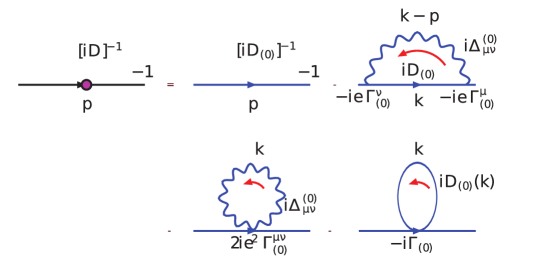
Figure 1: One-loop correction to the scalar propagator.

In this section we carry out a one-loop calculation of the scalar propagator with the standard approach. From the Lagrangian (6), we can read the corresponding Feynman rules

• For every vertex of one photon and two scalars $\phi_{A}$ and $\phi_{B}^{*}$, with momentum $P_{A}$ and $P_{B}$, respectively, we consider the factor $-ie\Gamma_{0}^{\mu}=-ie(P_{A}+P_{B})^{\mu}$.

• For the vertex of 2 photons labeled by the Lorentz indices $\mu$ and $\nu$, and two scalars $\phi_{A}$ and $\phi_{B}^{*}$, with momentum $P_{A}$ and $P_{B}$, respectively, we add a factor $2ie^{2}\Gamma_{0}^{\mu\nu}=2ie^{2}g^{\mu\nu}$.

• For a four-scalar vertex, a factor $-i\Gamma_{0}=-i\lambda$.

Moreover, for the internal lines we use the photon propagator (7) and the scalar propagator (8) in the diagrams shown in Fig. 1, corresponding to the one-loop correction to scalar propagator. In arbitrary space-time dimensions $d$, it corresponds to the following expression in Minkowski space

$$[iD^{(1)}_{d}(p;\xi)]^{-1} = [iD^{(0)}_{d}(p;\xi)]^{-1}-\int\frac{d^{d}k}{(2\pi)^{d}}[2ie^{2}\Gamma_{0}^{\mu\nu}][i\Delta_{\mu\nu}^{(0)}(k;\xi)]$$ (42)

$$-\int\frac{d^{d}k}{(2\pi)^{d}}[-ie\Gamma_{0}^{\mu}][iD_{d}^{(0)}(k;\xi)][-ie\Gamma_{0}^{\nu}][i\Delta_{\mu\nu}^{(0)}(k-p;\xi)]$$

$$-\int\frac{d^{d}k}{(2\pi)^{d}}[iD_{d}^{(0)}(k;\xi)][-i\Gamma_{0}]$$

$$= [iD^{(0)}_{d}(p;\xi)]^{-1}-I_{1}-I_{2}-I_{3}\;.$$

The integrals are divergent and thus require a regularization. It is customary to proceed within the dimensional regularization scheme DimReg , and we adopt this view for two different purposes: (i) To stick with the ordinary conventions of perturbative calculations in quantum field theory and (ii) to provide a link between the cut-off regularization of the LKFT scheme with this procedure. We start noticing that $I_{1}=0$, so, writing the explicit form of the remaining terms, we have that

$$[iD^{(1)}_{d}(p;\xi)]^{-1} = [iD^{(0)}_{d}(p;\xi)]^{-1}-i\lambda\int\frac{d^{d}k}{(2\pi)^{d}}\frac{1}{k^{2}-m^{2}}$$ (43)

$$-\int\frac{d^{d}k}{(2\pi)^{d}}(k+p)^{\nu}\frac{1}{k^{2}-m^{2}}(k+p)^{\mu}\frac{1}{q^{2}}\left[g_{\mu\nu}+(\xi-1)\frac{q_{\mu}q_{\nu}}{q^{2}}\right]\;.$$

$$=[iD^{(0)}_{d}(p;\xi)]^{-1}+(1-i\lambda)J_{01}+2(m^{2}+p^{2})J_{11}+2J_{10}+(m^{2}-p^{2})^{2}J_{21}\;,$$

where the master integral is

$$J_{np} = \int d^{d}k\frac{1}{(q^{2})^{n}(k^{2}-m^{2})^{p}}$$ (44)

$$=(-1)^{n+p}i\pi^{\frac{d}{2}}(m^{2})^{\frac{d}{2}-n-p}\frac{\Gamma\left(n+p-\frac{d}{2}\right)\Gamma\left(\frac{d}{2}-n\right)}{\Gamma(p)\Gamma\left(\frac{d}{2}\right)}\ _{2}F_{1}\left(-\frac{d}{2}+n+p,n;\frac{d}{2};\frac{p^{2}}{m^{2}}\right).$$

Details of the calculation of the above master integral (44) are presented in the appendix, because they correspond to standard perturbative calculations in quantum field theory. Upon substituting the appropriate values of $n$ and $p$, we are led to the final result for the one-loop correction to the scalar propagator,

$$[iD^{(1)}_{d}(p;\xi)]^{-1} = p^{2}-m^{2}-\left(\frac{m^{2}}{4\pi}\right)^{\frac{d}{2}}\frac{1}{m^{2}}\Gamma\left(1-\frac{d}{2}\right)$$ (45)

$$\times\Bigg{\{}e^{2}\Bigg{[}1-2\frac{(m^{2}+p^{2})}{m^{2}}\ _{2}F_{1}\left(2-\frac{d}{2},1;\frac{d}{2};\frac{p^{2}}{m^{2}}\right)$$

$$+(1-\xi)\frac{(m^{2}-p^{2})}{m^{4}}\ _{2}F_{1}\left(3-\frac{d}{2},2;\frac{d}{2};\frac{p^{2}}{m^{2}}\right)\Bigg{]}+\lambda\Bigg{\}}.$$

Let us consider some particular cases.

V.1 Three-dimensional case

Setting $d=3$ in Eq. (45) reduces the hypergeometric functions to transcendental, non divergent expressions, which after some manipulations can be expressed as

$$[iD^{(1)}_{3}(p;\xi)]^{-1}=p^{2}-m^{2}+\alpha\left[m-\frac{2(m^{2}+p^{2})}{m}\sqrt{\frac{m^{2}}{p^{2}}}\tanh^{-1}\sqrt{\frac{m^{2}}{p^{2}}}+(1-\xi)m\right]\;.$$ (46)

In order to compare against the results arising from the LKFT, we perform a Wick rotation to Euclidean space, such that.

$$[i{\cal D}^{(1)}_{3}(p;\xi)]^{-1}=-p^{2}-m^{2}+\alpha\left[m-2(m^{2}-p^{2})I(p,m)+(1-\xi)m\right]\;,$$ (47)

where we have defined

$$I(p,m)=\frac{1}{p}\arctan{\left(\frac{p}{m}\right)}\;.$$ (48)

The expression (47) is in agreement with its counterpart (18) to the leading term. The gauge independent terms cannot be derived from LKFT, as pointed our before. Moreover, in the massless limit, the propagator becomes

$${\cal D}^{(1)}_{3}(p;\xi)=\frac{1}{p^{2}+\alpha\pi p}\;,$$ (49)

which softens its infrared divergence from $1/p^{2}$ to $1/p$. We observe that the pole of this propagator is independent of $\xi$. Let us remark, as noticed earlier, that all the terms of the form $(\alpha\xi)^{n}$ are in agreement with the LKFT result (17).

Exercise: We encourage the students to use the expression (49) as input in the formula (25) to find the non perturbative form of the propagator in different gauges.

This concludes the discusion of the perturbative three-dimensional case. Next we consider the four-dimensional case.

V.2 Four-dimensional case

In $d=4$, in the expression for the propagator (45), the $\Gamma$ functions are divergent. We can easily expand these functions in powers of $\epsilon$ by taking $d=4^{*}$. Let us observe that when $d=4$, the hypergeometric functions reduce to

$${}_{2}F_{1}\left(2-\frac{d}{2},1;\frac{d}{2};\frac{p^{2}}{m^{2}}\right) = {}_{2}F_{1}\left(0,1;2;\frac{p^{2}}{m^{2}}\right)\ =\ 1$$ (50a)

$${}_{2}F_{1}\left(3-\frac{d}{2},2;\frac{d}{2};\frac{p^{2}}{m^{2}}\right) = {}_{2}F_{1}\left(1,2;2;\frac{p^{2}}{m^{2}}\right)\ =\ \frac{m^{2}}{p^{2}+m^{2}}\;,$$ (50b)

and thus the only divergence comes from

$$\Gamma\left(2-\frac{d}{2}\right) = \Gamma(\epsilon)\ =\ \frac{1}{\epsilon}+\mbox{finite}$$ (51a)

$$\Gamma\left(\frac{d}{2}-2\right) = \Gamma(-\epsilon)\ =\ -\frac{1}{\epsilon}+\mbox{finite}$$ (51b)

$$\Gamma\left(1-\frac{d}{2}\right) = \Gamma(-1+\epsilon)\ =\ -\frac{1}{\epsilon}+\mbox{finite}\;,$$ (51c)

such that when $d=4^{*}$,

$$\left[D_{4^{*}}^{(1)}(p;\xi)\right]^{-1}=p^{2}-m^{2}-\frac{\alpha}{4\pi\epsilon}\left[m^{2}+2p^{2}-(1-\xi)(m^{2}-p^{2})\right]+\mbox{finite.}$$ (52)

This expression encodes the leading divergence, which corresponds to the divergence of the propagator when $\Lambda\to\infty$ in Eq. (41). We can improve on our understanding of the propagator by identifying the finite piece in Eq. (52). For this purpose, we resort to the software HypExp ; NumExp to expand the hypergeometric functions in $d=4^{*}$. Here we simply quote the result and leave the details as an exercise to the reader,

$$\left[{\cal D}_{4^{*}}^{(1)}(p;\xi)\right]^{-1} = p^{2}-m^{2}-\frac{m^{2}}{(4\pi^{2})}\frac{1}{\epsilon}\Bigg{[}4\pi\alpha+\lambda+\frac{4\pi\alpha}{m^{2}}\bigg{[}-2(m^{2}+p^{2})+(1-\xi)(m^{2}-p^{2})\bigg{]}\Bigg{]}$$ (53)

$$+\frac{m^{2}}{(4\pi)^{2}}\Bigg{[}C\Bigg{(}4\pi\alpha+\lambda+\frac{4\pi\alpha}{m^{2}}\bigg{[}-2(m^{2}+p^{2})+(1-\xi)(m^{2}-p^{2})\bigg{]}\Bigg{)}$$

$$+4\pi\alpha\Bigg{[}-2\frac{(m^{2}+p^{2})}{m^{2}}\left(1-\frac{p^{2}-m^{2}}{p^{2}}\ln\left(1-\frac{p^{2}}{m^{2}}\right)\right)\Bigg{]}$$

$$-4\pi\alpha(1-\xi)\frac{(m^{2}-p^{2})}{m^{2}}\left(1-\frac{p^{2}-m^{2}}{p^{2}}\ln\left(1-\frac{p^{2}}{m^{2}}\right)\right)\Bigg{\}}\;,$$

where

$$C=1-\gamma_{E}-\ln\left(\frac{m^{2}}{4\pi}\right)\;.$$ (54)

It is not difficult to convince oneself that the gauge dependent terms in Eq. (53) exactly match those in Eq. (41), and that the only difference comes from the $\xi$-independent terms, a difference allowed by the structure of LKFTs.

Exercise: We encourage graduate students to perform the intermediate steps to obtain the expression (53). The expansion of the hypergeometric functions is not trivial, so we provide the following results

$${}_{2}F_{1}\left(\epsilon,1;2-\epsilon;\frac{p^{2}}{m^{2}}\right) = 1+\epsilon\Bigg{[}1-\frac{p^{2}-m^{2}}{p^{2}}\ln\left(1-\frac{p^{2}}{m^{2}}\right)\Bigg{]}+{\cal O}(\epsilon^{2})$$ (55a)

$${}_{2}F_{1}\left(1+\epsilon,2;2-\epsilon;\frac{p^{2}}{m^{2}}\right) = \frac{m^{2}}{m^{2}-p^{2}}\Bigg{[}1-\epsilon\left(1-\frac{p^{2}-m^{2}}{p^{2}}\ln\left(1-\frac{p^{2}}{m^{2}}\right)\right)\Bigg{]}$$

$$+{\cal O}(\epsilon^{2})$$ (55b)

VI Conclusions

We have derived a non-perturbative expression for the scalar propagator in SQED through its LKF transformation, starting from its tree level expression in 3 and 4 space-time dimensions. Equations (16) and (31) display two of the main results of this paper. The LKFT of the scalar propagator is written entirely in terms of basic functions of momentum. Although our input is merely the bare propagator, its LKFT, being non-perturbative in nature, contains useful information of higher orders in perturbation theory. All the coefficients of the $(\alpha\xi)^{i}$ at every order are correctly reproduced without ever having to perform loop calculations. In the weak coupling regime, LKFT results match onto the one-loop perturbative results derived from the Lagrangian (6) up to gauge independent terms, a difference allowed by the structure of the LKFT. This difference arises due to our approximate input, and can be systematically removed at the cost of employing a more complex input which would need to be calculated by the brute force of perturbation theory.

Appendix

In this appendix we calculate the master integral (44). Using the identity

$$\frac{1}{A^{n}B^{p}}=\frac{\Gamma(n+p)}{\Gamma(n)\Gamma(p)}\int_{0}^{1}dx\frac{x^{n-1}(1-x)^{p-1}}{[xA+(1-x)B]^{n+p}}\;,$$ (56)

we have

$$J_{np}=\frac{\Gamma(n+p)}{\Gamma(n)\Gamma(p)}\int_{0}^{1}dx\int d^{d}k\frac{x^{n-1}(1-x)^{p-1}}{[x(k-p)^{2}+(1-x)(k^{2}-m^{2})]^{n+p}}\;.$$ (57)

We need to transform the denominator in a convenient form to use dimensional regularization results. Let

$$D = x(k-p)^{2}+(1-x)(k^{2}-m^{2})$$ (58)

$$= x[k^{2}+p^{2}-2k\cdot p]+(1-x)k^{2}-m^{2}(1-x)$$

$$= k^{2}-2k\cdot px+p^{2}x-m^{2}(1-x)\;.$$

Now we perform the change of variables

$$w=k-px\;\qquad\Rightarrow\qquad k=w+px\;.$$ (59)

Thus, replacing Eq. (59) into Eq. (58) we have that

$$D = (w+px)^{2}-2(w+px)\cdot px+p^{2}x-m^{2}(1-x)$$ (60)

$$= w^{2}+p^{2}x(1-x)-m^{2}(1-x)\;.$$

Substituting Eq. (60), from Eq. (57) we have

$$J_{np}=\frac{\Gamma(n+p)}{\Gamma(n)\Gamma(p)}\int dxx^{n-1}(1-x)^{p-1}\int d^{d}w\frac{1}{[w^{2}+p^{2}x(1-x)-m^{2}(1-x)]}\;.$$ (61)

This expression is of the form

$$\int\frac{d^{d}w}{(w^{2}+s)^{n}}=i\pi^{d/2}\frac{\Gamma(n-\frac{1}{2}d)}{\Gamma(n)}\frac{1}{s^{n-d/2}}\;,$$ (62)

with $s=p^{2}x(1-x)-m^{2}(1-x)$, and therefore we can write (61) as

$$J_{np} = \frac{(-1)^{n+p}i\pi^{d/2}\Gamma(n+p-\frac{d}{2})}{\Gamma(n)\Gamma(p)}\int_{0}^{1}dx[-p^{2}x(1-x)+m^{2}(1-x)]^{\frac{d}{2}-n-p}\times$$ (63)

$$x^{n-1}(1-x)^{p-1}\;.$$

Performing the integration,

$$\int_{0}^{1}dx[-p^{2}x(1-x)+m^{2}(1-x)]^{\frac{d}{2}-n-p}x^{n-1}(1-x)^{p-1}=$$ (64)

$$= \int_{0}^{1}x^{n-1}(1-x)^{p-1}(1-x)^{\frac{d}{2}-n-p}(-p^{2}x+m^{2})^{\frac{d}{2}-n-p}dx$$

$$= (m^{2})^{\frac{d}{2}-n-p}\int_{0}^{1}x^{n-1}(1-x)^{\frac{d}{2}-n-1}(1-\frac{p^{2}}{m^{2}}x)^{\frac{d}{2}-n-p}dx$$

Next, we use

$$\int_{0}^{1}x^{\lambda-1}(1-x)^{\mu-1}(1-\beta x)^{-\nu}dx=B(\lambda,\mu){}_{2}F_{1}(\nu,\lambda;\lambda+\mu;\beta)\;,$$ (65)

where $\lambda=n$, $\mu=\frac{d}{2}-n$, $\beta=\frac{p^{2}}{m^{2}}$ y $-\nu=\frac{d}{2}-n-p$. Thus,

$$\int_{0}^{1}x^{n-1}(1-x)^{\frac{d}{2}-n-1}(1-\frac{p^{2}}{m^{2}}x)^{\frac{d}{2}-n-p}dx=$$ (66)

$$= B\bigg{(}n,\frac{d}{2}-n\bigg{)}{}_{2}F_{1}\bigg{(}-\frac{d}{2}+n+p,n;\frac{d}{2};\frac{p^{2}}{m^{2}}\bigg{)}$$

$$= \frac{\Gamma(n)\Gamma(\frac{d}{2}-n)}{\Gamma(\frac{d}{2})}{}_{2}F_{1}\bigg{(}-\frac{d}{2}+n+p,n;\frac{d}{2};\frac{p^{2}}{m^{2}}\bigg{)}\;.$$

Finally

$$J_{np} = (-1)^{n+p}i\pi^{d/2}(m^{2})^{\frac{d}{2}-n-p}\frac{\Gamma(n+p-\frac{d}{2})\Gamma(\frac{d}{2}-n)}{\Gamma(p)\Gamma(\frac{d}{2})}\times$$ (67)

$${}_{2}F_{1}\bigg{(}-\frac{d}{2}+n+p,n;\frac{d}{2};\frac{p^{2}}{m^{2}}\bigg{)}\;.$$

References

- (1) R. Mills,“Gauge Fields”, Am. J. Phys. 57, 493-507 (1989); J.D. Jackson and L.B. Okun, “Historical roots of gauge invariance”, Rev. Mod. Phys. 63, 663-680 (2001).
- (2) J.D. Jackson, “From Lorentz to Coulomb and other explicit gauge transformations”, Am. J. Phys. 70, 917-928 (2002).
- (3) B.R. Holstein, “Gauge invariance and quatization”, Am. J. Phys. 56, 425-429 (1988).
- (4) D.L. Karatas and K.L. Kowalski, “Noether’s theorem for local gauge transformations”, Am. J. Phys. 58, 123-131 (1990); H. A. Al-Kuwuari and M.O. Taha, “Noether’s theorem and local gauge invariance”, Am. J. Phys. 59, 363-365 (1991).
- (5) P.B. Pal and K.S. Sateesh, “The field strength and the Lagrangian of a gauge theory”, Am. J. Phys. 58, 789-790 (1990).
- (6) E. Corinaldesi and P. Roman, “Operator gauge transformations”, Am. J. Phys. 33, 939-942 (1965).
- (7) J.C. Ward, “An identity in quantum electrodynamics”, Phys. Rev. 78 182-182 (1950); H.S. Green, “A pre-renormalized quantum electrodynamics”, Proc. Phys. Soc. (London) A66 873-880 (1953); Y. Takahashi, “On the generalized Ward identity”, Nuovo Cimento 6 371-375 (1957).
- (8) N.K. Nielsen, “On the gauge dependence of spontaneous symmetry breaking in gauge theories”, Nucl. Phys. B101 173-188 (1975); O. Piguet and K. Sibold, “Gauge independence in ordinary Yang-Mills theories”, Nucl. Phys. B253 517-540 (1985).
- (9) J.C. Breckenridge, M.J. Lavelle and T.G. Steele, “The Nielsen identities for the two poijnt functions of QED and QCD”, Z. Phys. C65 155-164 (1995); P. Gambino and P.A. Grassi, Phys. Rev. D62 076002, 17pp. (2000).
- (10) L.D. Landau and I.M. Khalatnikov, “The gauge transformation of the Green function for charged particles”, Zh. Eksp. Teor. Fiz. 29 89-93 (1956), Sov. Phys. JETP 2 69-73 (1956); E.S. Fradkin, “Concerning some general relations of quantum electrodynamics”, Zh. Eksp. Teor. Fiz. 29, 258-261(1955), Sov. Phys. JETP 2, 361-363 (1956).
- (11) K. Johnson and B. Zumino, “Gauge dependence of wave-function renormalization constant in quantum electrodynamics”, Phys. Rev. Lett. 3 351-352 (1959); B. Zumino, “Gauge properties of propagators in quantum electrodynamics”, J. Math. Phys. 1 1-7 (1960); S. Okubo, “The gauge properties of Green’s functions in quantum electrodynamics”, Nuovo Cim. 15 949-958 (1960); I. Bialynicki-Birula, “On the gauge properties of Green’s functions”, Nuovo Cim. 17 951 (1960); T.K. Gaisser, “Operator gauge transformations and gauge transformations of the third kind”, Am. J. Phys. 34, 597 (1966); H. Sonoda, “On the gauge parameter dependence of QED”, Phys. Lett. B499, 253-260 (2001).
- (12) K. Wilson, “Confinement of quarks”, Phys. Rev. D10, 2445-2459 (1974); M. Creutz, Quarks, gluons and lattices, Cambridge University Press 1985;
- (13) J. Gasser and H. Leutwyler, “Chiral perturbation theory to one-loop”, Ann. Phys. 158, 142-210 (1984); J. Gasser and H. Leutwyler, “Chiral perturbation theory: Expansions in the mass of the strange quark”, Nucl. Phys. B 250, 465-516 (1985); G. Ecker, J. Gasser, A. Pich and E. de Rafael, “The role of resonances in chiral perturbation theory”, Nucl. Phys. B 321, 311-342 (1989); U. G. Meissner, “Recent developments in chiral perturbation theory”, Rept. Prog. Phys. 56, 903-996 (1993); A. Pich, “Chiral perturbation theory”, Rep. Prog. Phys. 58 563-610 (1995); G. Ecker, “Chiral perturbation theory”, Prog. Part. Nucl. Phys. 35, 1-80 (1995).
- (14) F. J. Dyson, “The matrix in quantum electrodynamics”, Phys. Rev. 75 1736-1755 (1949); J. S. Schwinger, “On the Green’s functions of quantized fields. 1.” Proc. Nat. Acad. Sc. 37, 452-455 (1951).
- (15) I.G. Aznauryan et. al., “Studies of Nucleon Resonance Structure in Exclusive Meson Electroproduction”, Int. J. Mod. Phys. E 22, 1330015 (2013); A. Bashir et. al., “Collective perspective on advances in Dyson-Schwinger Equation QCD”, Commun. Theor. Phys. 58, 79-134 (2012).
- (16) K. Raya, A. Bashir, S. Hern ndez-Ortiz, A. Raya and C.D. Roberts, “Multiple solutions for the fermion mass function in QED3”, Phys. Rev. D 88, 096003 (2013); A. Bashir, A. Raya, S. Sanchez-Madrigal and C.D. Roberts, “Gauge invariance of a critical number of flavours in QED3”, Few Body Syst. 46, 229-237 (2009); A. Bashir and A. Raya, “Truncated Schwinger-Dyson equations and gauge covariance in QED3”, Few Body Syst. 41, 185-199 (2007); A. Bashir and Raya, “Gauge symmetry and its implications for the Schwinger-Dyson equations”, in Trends in Boson Research 1st edn. editor A. V. Ling (New York.: Nova Science Publishers) pp. 183 229 ISBN 1-59454-521-9 (2006); A. Bashir and A. Raya, “Dynamical fermion masses and constraints of gauge invariance in quenched QED(3)”, Nucl. Phys. B709 307-328 (2005); C. S. Fischer, R. Alkofer, T. Dahm and P. Maris, “Dynamical chiral symmetry breaking in unquenched QED3”, Phys. Rev. D 70, 073007, 20pp. (2004); A. Bashir, A. Kizilersu, M. R. Pennington, “Does the weak coupling limit of the Burden-Tjiang deconstruction of the massless quenched three-dimensional QED vertex agree with perturbation theory?”, Phys. Rev. D 62 085002 (2000).
- (17) A. Bashir, Y. Concha-Sanchez, Robert Delbourgo, “3-point off-shell vertex in scalar QED in arbitrary gauge and dimension”, Phys. Rev. D 76 065009 (2007); On the Compton scattering vertex for massive scalar QED A. Bashir, Y. Concha-Sanchez, R. Delbourgo, M.E. Tejeda-Yeomans, Phys. Rev. D 80 045007 (2009).
- (18) R. Delbourgo and B.W. Keck, “On the gauge dependence of spectral functions”, J. Phys. A13 701-712 (1980); R. Delbourgo, B.W. Keck and C.N. Parker, “Gauge covariance and the gauge technique”, J. Phys. A14 921-930 (1981).
- (19) A. Bashir, “Nonperturbative fermion propagator for the massless quenched QED3”, Phys. Lett. B491 280-284 (2000).
- (20) A. Bashir and A. Raya, “Landau-Khalatnikov-Fradkin transformations and the fermion propagator in quantum electrodynamics”, Phys. Rev. D66 105005, 8pp. (2002).
- (21) A. Bashir and A. Raya, “Fermion propagator in quenched QED3 in the light of the Landau-Khalatnikov-Fradkin transformations”, Nucl. Phys. Procc. Suppl. 141, 259-264 (2005).
- (22) A. Bashir and R. Delbourgo, “The nonperturbative propagator and vertex in massless quenched QED(d)”, J. Phys. A37 6587-6598 (2004).
- (23) R.D. Pisarski, “Chiral symmetry breaking in three-dimensional electrodynamics”, Phys. Rev. D29, 2423-2426 (1984); A. Ayala, A. Bashir, “Dynamical mass generation for fermions in quenched quantum electrodynamics at finite temperature”, Phys. Rev. D 67, 076005 (2003).
- (24) L. D. Landau, “Paramagnetism of metals”, Z. Phys. 64, 629 637 (1930).
- (25) F. Wilczek, Fractional Statistics and Anyon Superconductivity (World Scientific, Singapore, 1998); A. Khare, Fractional Statistics and Quantum Theory (World Scientific, Singapore, 2005), 2nd ed.
- (26) N. Dorey and N. E. Mavromatos, “QED and three dimensions and two-dimensional superconductivity without parity violation”, Nucl. Phys. B386, 614-682 (1992); G. Triantaphyllou, “Dynamical mass generation in a finite temperature Abelian gauge theory”, Phys. Rev. D58, 065006, 7pp. (1998).
- (27) F. Olness and R. Scalise, “Regularization, renormalization, and dimensional analysis: Dimensional regularization meetsfreshman E&M”, Am. J. Phys. 79, 306-312 (2011).
- (28) T. Hubber and D. Maître, “HypExp, a Mathematica package for expanding hypergeometric functions around integer-valued parameters”, Comput. Phys. Commun. 175, 122-144 (2006); T. Hubber and D. Maître, “HypExp 2, Expanding Hypergeometric Functions about Half-Integer Parameters”, Comput. Phys. Commum. 178, 755-776 (2008).
- (29) Z.-W. Huang and J. Liu, “NumExp: Numerical epsilon expansion of hypergeometric functions”, Comput. Phys. Commum. 184, 1973-1980 (2013).