Charm quark mass and D-meson decay constants from two-flavour lattice QCD

Abstract:

We present a computation of the charm quark’s mass and the leptonic D-meson decay constants $f_{{\rm D}}$ and $f_{{\rm D}_{\rm s}}$ in two-flavour lattice QCD with non-perturbatively O($a$) improved Wilson quarks. Our analysis is based on the CLS configurations at two lattice spacings ($a=0.065$ and $0.048$ fm, where the lattice scale is set by $f_{{\rm K}}$) and pion masses ranging down to $\sim 190$ MeV at $Lm_{\pi}\gtrsim 4$, in order to perform controlled continuum and chiral extrapolations with small systematic uncertainties.

1 Introduction

The decay constants $f_{\rm D}$ and $f_{\rm D_{\rm s}}$ entering the Standard Model expression for the leptonic decay widths of charged D-mesons are given by the non-perturbative QCD matrix elements

$$\langle 0|\overline{q}\gamma_{\mu}\gamma_{5}c|{\rm D}_{q}(p)\rangle={\rm i}{f_{\rm D}}_{q}\,p_{\mu}\;,\quad q={\rm d},{\rm s}\;.$$ (1)

Besides the importance of ${f_{\rm D}}_{q}$ in extracting $|V_{{\rm c}q}|$ and overconstraining the CKM matrix, there is continuing phenomenological interest in these decays, because a significant deviation between experimental and lattice results for ${f_{\rm D}}_{q}$ could hint at New Physics in the flavour sector [1]. Extending our previous work [2] with an expanded set of ensembles with higher statistics, lighter sea quarks and largely reduced systematics (such as the uncertainty in the lattice scale), we here report results of a preliminary analysis of $f_{{\rm D}_{\rm(s)}}$ and of the charm quark mass.

2 Computational setup and techniques

Our measurements were performed on a subset of the Coordinated Lattice Simulations (CLS) gauge field ensembles, which are characterized by the Wilson plaquette gauge action and a sea of $N_{\rm f}=2$ mass degenerate flavours of non-perturbatively ${\rm O}(a)$ improved Wilson quarks. The sea quark masses span a range corresponding to pion masses $(190\lesssim m_{\pi}\lesssim 440)\,{\rm MeV}$, while the strange valence quark is fixed to its physical value and we scan a range of charm valence quark masses around the physical charm quark mass. Two values of the lattice spacing are considered: $a\in\{0.065\,{\rm fm}\,,\,0.048\,{\rm fm}\}$. Suppression of finite-size effects is ensured by restricting ourselves to ensembles with $Lm_{\pi}\gtrsim 4$. To generate the gauge configurations, either the DD-HMC [3, 4, 5, 6] or the MP-HMC based on mass preconditioning [7, 8] was employed. The parameters of the ensembles used are summarized in table 1. Statistical errors are estimated via a jackknife procedure, but will be double-checked in the final analysis by the method of [9] studying autocorrelation functions.

id	$L/a$	$\beta$	$a\,[\,{\rm fm}\,]$	$\kappa_{\rm l}$	$\kappa_{\rm s}$	$m_{\pi}\,[\,{\rm MeV}\,]$	# cfgs
E5	$32$	5.3	0.065	$0.136250$	$0.135777(17)$	440	$2\times 199$
F6	$48$			$0.136350$	$0.135741(17)$	310	250
F7	$48$			$0.136380$	$0.135730(17)$	270	547
G8	$64$			$0.136417$	$0.135705(17)$	190	820
N5	$48$	5.5	0.048	$0.136600$	$0.136262(08)$	440	238
N6	$48$			$0.136670$	$0.136250(08)$	340	1000
O7	$64$			$0.136710$	$0.136243(08)$	270	486

Table 1: Parameters of the ensembles used: ensemble label, spatial extent of the lattice in lattice units, bare coupling $\beta=6/g_{0}^{2}$, lattice spacing $a$, hopping parameters of the sea and (valence) strange quarks, the mass of the sea pion and the number of configurations employed. All lattices have dimensions $T\times L^{3}$ with $T=2L$.

The lattice spacings $a$, pion masses $m_{\pi}$, pion decay constants $f_{\pi}$ and values of the (quenched) strange quark’s hopping parameter $\kappa_{\rm s}$ are inferred from [10], where the scale is set through $f_{\rm K}$ at the “physical point” defined by $m_{\pi,{\rm phys}}=134.8\,{\rm MeV}$, $m_{{\rm K},{\rm phys}}=494.2\,{\rm MeV}$ and $f_{{\rm K},{\rm phys}}=155\,{\rm MeV}$ in the isospin-symmetric limit with QED effects removed. For two ensembles (G8,N6), we had to perform a short linear interpolation in $1/\kappa_{\rm s}$ (at fixed charmed $\kappa_{\rm c}$) to the physical value.

As for the hopping parameter of the (quenched) charm quark, $\kappa_{\rm c}$, we fix it by requiring the ${\rm D}_{\rm s}$-meson mass to acquire its physical value, $m_{\rm D_{\rm s}}=m_{{\rm D_{\rm s}},{\rm phys}}=1968\,{\rm MeV}$, irrespective of the sea quark mass. To this end, after choosing a few values in the vicinity of this target, $(am_{\rm D_{\rm s}})^{2}$ was interpolated linearly in $1/\kappa_{\rm c}$ to $(am_{{\rm D_{\rm s}},{\rm phys}})^{2}$.

3 Observables and analysis details

For two mass non-degenerate valence quarks $r$ and $s$, we compute correlators of the pseudoscalar density $P^{rs}=\overline{\psi}_{r}\gamma_{5}\psi_{s}$ and the time component of the axial vector current $A_{0}^{rs}=\overline{\psi}_{r}\gamma_{0}\gamma_{5}\psi_{s}$ as

$$f_{\rm PP}^{rs}(x_{0})=-a^{3}\sum_{\vec{x}}\langle P^{rs}(x)P^{sr}(0)\rangle\;,\quad f_{\rm AP}^{rs}(x_{0})=-a^{3}\sum_{\vec{x}}\langle A_{0}^{rs}(x)P^{sr}(0)\rangle\;.$$ (2)

These are evaluated using 10 $U(1)$ noise sources $\eta_{t}(x)=\delta_{t,x_{0}}\exp(i\phi(\vec{x}))$ located on randomly chosen time slices $t$ [11, 12] so that solving the Dirac equation once for each noise vector $\zeta_{t}^{r}=Q^{-1}(m_{0,r})\eta_{t}=a^{-1}(D+m_{0,r})^{-1}\gamma_{5}\eta_{t}$ suffices to estimate the two-point functions projected onto zero momentum:

$$a^{3}f_{\rm XP}^{rs}(x_{0})={\textstyle\sum_{\vec{x}}}\,\langle[\zeta_{t}^{r}(x_{0}+t,\vec{x})]^{\dagger}\Gamma\zeta_{t}^{s}(x_{0}+t,\vec{x})\rangle\;,\quad\mbox{$\Gamma={\bf 1},\gamma_{0}$ for ${\rm X}={\rm P,A}$}\;,$$ (3)

where the average is over noise sources and gauge configurations.

The ${\rm O}(a)$ improved effective average PCAC quark mass of flavours $r$ and $s$ is now defined as

$${\textstyle{\frac{1}{2}}}\,(m_{rr}+m_{ss})(x_{0})=m_{rs}(x_{0})=\frac{\frac{1}{2}\,(\partial_{0}+\partial_{0}^{*})f_{\rm AP}(x_{0})+c_{\rm A}\,a\,\partial_{0}^{*}\partial_{0}f_{\rm PP}(x_{0})}{2f_{\rm PP}(x_{0})}\;,$$ (4)

where the improvement coefficient $c_{\rm A}$ is non-perturbatively known from [13]. For sufficiently large $x_{0}$, $m_{rs}(x_{0})$ exhibits a plateau, over which we take a timeslice average to calculate $m_{rs}$. Examples for two representative ensembles and various valence $\kappa$–combinations are shown in figure 1.

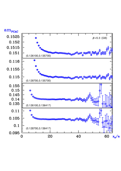
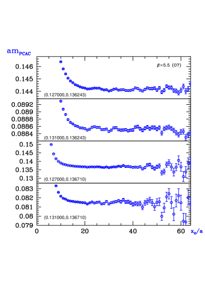
Figure 1: Local PCAC quark masses for representative charm-strange (upper 2 panels) and charm-light (lower 2 panels) $\kappa$–combinations for the G8 and O7 ensembles. Our bare quark mass estimates are obtained as averages over the plateau regions.

The renormalized PCAC mass is then given by

$$m_{{{\rm R}}}^{rs}=\frac{Z_{\rm A}(1+\bar{b}_{\rm A}am_{\mathrm{sea}}+\tilde{b}_{\rm A}am_{rs})}{Z_{\rm P}(1+\bar{b}_{\rm P}am_{\mathrm{sea}}+\tilde{b}_{\rm P}am_{rs})}\times m_{rs}\;,\quad\mbox{$m_{\mathrm{sea}}=m_{{\rm l}{\rm l}}$ with ${\rm l}={\rm l(ight)}$}\;,$$ (5)

where $Z_{\rm A}$ and $Z_{\rm P}$ assume values from the non-perturbative determinations in [10, 14, 15, 16]). The $b$–coefficients, multiplying (very small) improvement terms, are known in 1-loop perturbation theory [10, 17]; in particular, $\bar{b}_{\rm A}=\bar{b}_{\rm P}=0$ holds at this order.

Expressions for the pseudoscalar (PS) meson mass and its decay constant arise from the spectral decomposition for infinite $T$,

$$f_{\rm PP}(x_{0})={\textstyle\sum_{i=1}^{\infty}}\,c_{i}\,{\rm e}^{\,-E_{i}x_{0}}\;,\quad E_{1}=m_{\rm PS}\;,\quad\mbox{$E_{i\geq 2}$: excited states contributions}\;,$$ (6)

which decays exponentially for large time separations. In this asymptotic regime, the decay constant is thus given by:

$$f_{\rm PS}=Z_{\rm A}\,(1+\bar{b}_{\rm A}am_{\mathrm{sea}}+\tilde{b}_{\rm A}am_{rs})\times f_{\rm PS}^{\rm bare}\;,\quad f_{\rm PS}^{\rm bare}=2\sqrt{2c_{1}}\,m_{rs}\,m_{\rm PS}^{-3/2}\;.$$ (7)

Since in the actual analysis we face finite time extents $T$ and separations $x_{0}$, and hence particles running backwards in time and excited states, we employ the following two-step procedure to fix the region $x_{0}\in[x_{0}^{\rm min},T-x_{0}^{\rm min}]$, in which the excited state contribution to $f_{\rm PP}$ can be neglected: 1.) Determine $x_{0}^{\rm min}$ as the smallest $x_{0}$, where the excited state, estimated by a 2-state fit (including finite-$T$ effects) to $f_{\rm PP}(x_{0})=c_{1}\big{[}{\rm e}^{-E_{1}x_{0}}+{\rm e}^{-E_{1}(T-x_{0})}\big{]}+c_{2}\big{[}{\rm e}^{-E_{2}x_{0}}+{\rm e}^{-E_{2}(T-x_{0})}\big{]}$, contributes less than $1/4$ of the statistical uncertainty on the effective mass $M_{\rm eff}(x_{0})$; here the effective PS meson mass $M_{\rm eff}$ is defined as $\cosh\left[M_{\rm eff}(x_{0}-T/2)\right]/\cosh\left[M_{\rm eff}(x_{0}+1-T/2)\right]=f_{\rm PP}(x_{0})/f_{\rm PP}(x_{0}+1)$. 2.) Perform a 1-state fit of the asymptotic exponential decay, restricted to this region, to extract $m_{\rm PS}=E_{1}$ and the leading coefficient $c_{1}$, eventually entering the evaluation of the decay constants according to eq. (7). This is illustrated for our most chiral ensemble in figure 2.

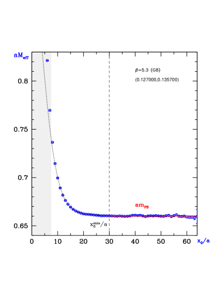
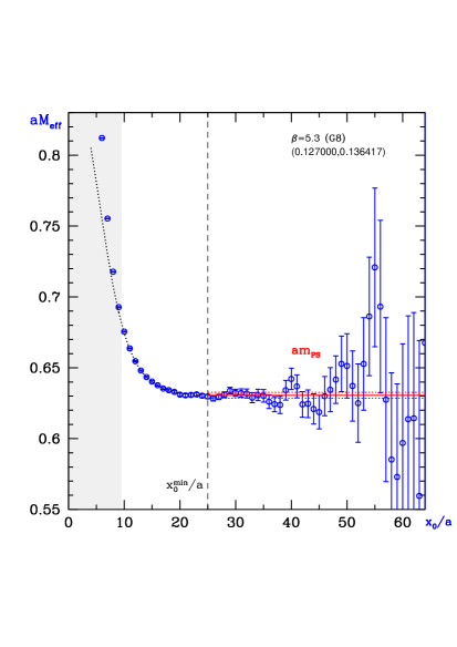
Figure 2: The effective mass in the pseudoscalar channel extracted from $f_{\rm PP}$ for a representative charm-strange (left) and charm-light (right) $\kappa$–combination for the G8 ensemble. A two-state fit to data outside the shaded area, where the fit function describes the data well given their accuracy, determines $x_{0}^{\rm min}$. The result of the final one-state fit is given by the error band.

4 Preliminary results

Unphysical pion masses and non-zero lattice spacings in our data are accounted for by employing joint chiral ($m_{\pi}\to m_{\pi,{\rm phys}}=134.8\,{\rm MeV}$) and continuum limit ($a\to 0$) extrapolations.

Assuming a linear dependence on the squared (sea) pion mass, our fit ansatz for the renormalized PCAC quark mass composed of a charm and a light valence flavour ($s={\rm s},{\rm l}$) reads

$$m_{{{\rm R}}}^{{\rm c}s}\left(m_{\pi},a\right)=B+Cm_{\pi}^{2}+Da^{2}\;.$$ (8)

In addition, we also consider the definition via the bare subtracted quark mass, $m_{{\rm q},{\rm c}}=m_{0,{\rm c}}-m_{\rm crit}$, so that we have three ways to obtain the renormalization group invariant (RGI) charm quark mass, $M_{\rm c}$ [18, 19]:

$${\textstyle{\frac{1}{2}}}\,(M_{\rm c}+{M}_{s})=\frac{M}{\kern 1.0pt\overline{\kern-1.0ptm\kern-1.0pt}\kern 1.0pt}\,m_{{{\rm R}}}^{{\rm c}s}\;;\quad M_{\rm c}=\frac{M}{\kern 1.0pt\overline{\kern-1.0ptm\kern-1.0pt}\kern 1.0pt}\,\frac{Z_{\rm A}}{Z_{\rm P}}\,Z\left(1+b_{\rm m}am_{{\rm q},{\rm c}}\right)m_{{\rm q},{\rm c}}\;,\quad m_{{\rm q},{\rm c}}=\frac{1}{2}\Big{(}\frac{1}{\kappa_{\rm c}}-\frac{1}{\kappa_{\rm crit}}\Big{)}\;.$$ (9)

The universal factor $M/\kern 1.0pt\overline{\kern-1.0ptm\kern-1.0pt}\kern 1.0pt$, which translates the running mass at a given scale to the RGI one, as well as the other renormalization and improvement factors entering here, are non-perturbatively known from [10, 14, 15, 16]. The combined $m_{\pi}^{2}$– and $a^{2}$–dependence of the three definitions in eq. (9) is shown in the left panel of figure 3 to lead to consistent results in the joint chiral and continuum limit. A more careful error analysis still to come, we consider the spread of these values as an upper limit for the overall uncertainty and quote as preliminary estimate for the charm quark’s mass

$$M_{\rm c}=1.51(4)\,{\rm GeV}\quad\Rightarrow\quad\overline{m}_{\rm c}^{\,\overline{\rm MS}}\big{(}\overline{m}_{\rm c}^{\,\overline{\rm MS}}\big{)}=1.274(36)\,{\rm GeV}\;,$$ (10)

where $M_{\rm s}$ from [10] and in the conversion to the $\overline{\rm MS}$ scheme the known 4-loop anomalous dimensions of quark masses and coupling [20, 21] together with $\Lambda_{\overline{{\rm MS}}}$ from [10] were used.

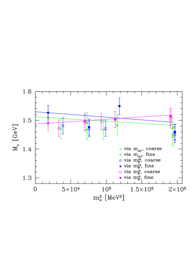
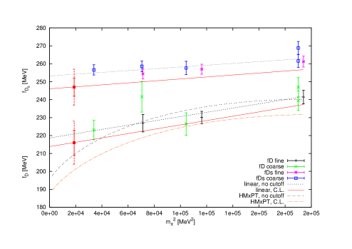
Figure 3: Left: Joint chiral and continuum extrapolation of the RGI mass of the charm quark, using the definitions via the heavy-light PCAC relation (where $s={\rm s},{\rm l}$) and via the bare subtracted mass, eq. (9). Right: Joint chiral and continuum extrapolations to the physical point of $f_{\rm D}$ and $f_{\rm D_{\rm s}}$ to the fit ansätze in eqs. (11) and (12). Labels “coarse” and “fine” refer to $\beta=5.3$ and $5.5$, respectively, and for $f_{\rm D_{(s)}}$ also fits neglecting cutoff effects are displayed.

For the D-meson decay constants, we adopt again fit ansätze linear in $m_{\pi}^{2}$ (and $a^{2}$), while for $f_{\rm D}$ we also model the sea quark dependence in a fit form inspired by partially quenched heavy meson chiral perturbation theory ($\mbox{HM}\chi\mbox{PT}$) [22, 23], treating the charm quark as heavy, viz.

$$f_{\rm D_{(s)}}\left(m_{\pi},a\right) = b_{\rm(s)}+c_{\rm(s)}\,m_{\pi}^{2}+d_{\rm(s)}\,a^{2}\;,$$ (11)

$$f_{\rm D}\left(m_{\pi},a\right) = b^{\prime}\left[1-\frac{3}{4}\,\frac{1+3\,\hat{g}^{2}}{(4\pi f_{\pi})^{2}}\,m_{\pi}^{2}\ln\big{(}m_{\pi}^{2}\big{)}\right]+c\,^{\prime}m_{\pi}^{2}+d\,^{\prime}\,a^{2}\;;$$ (12)

$m_{\rm s}$–terms are assumed to be absorbed into the ${\rm O}(m_{\pi}^{0})$ constants, because we work at fixed physical strange quark mass, and $\widehat{g}=g_{{\rm D}^{*}{\rm D}\pi}=0.6$ [24] is the ${\rm D}^{*}{\rm D}\pi$–coupling. These combined chiral and continuum extrapolations to the physical point are depicted in the right panel of figure 3. As can be seen from the fits, our data for $f_{\rm D}$ are best described by the linear extrapolation along eq. (11), and we do not see any evidence for the significance of the chiral logarithm-term in eq. (12). Therefore, we take the linear extrapolations as the central values to arrive at our present results

$$f_{\rm D_{s}}=247(5)_{\rm stat}(5)_{\rm syst}\,{\rm MeV}\;,\quad f_{\rm D}=216(7)_{\rm stat}(5)_{\rm syst}\,{\rm MeV}\;,\quad f_{\rm D_{s}}/f_{\rm D}=1.14(2)_{\rm stat}(3)_{\rm syst}$$ (13)

and the difference to the $\mbox{HM}\chi\mbox{PT}$ fit to account for a part of the systematic error of $f_{\rm D}$. Apart from the statistical errors, the quoted uncertainties also contain a conservative estimate of the contribution from the scale setting.

5 Conclusions and outlook

The results for the charm quark mass and the D-meson decay constants from our analysis are very well in line with computations of other groups, see, e.g., the recent summaries in [25, 26]. Note that by setting the scale through $f_{\rm K}$ we effectively compute $f_{\rm D_{(s)}}/f_{\rm K}$, where $Z_{\rm A}$ in eq. (7) (and thus also its error) drops out, but that it still re-enters indirectly by also fixing $\kappa_{\rm s},\kappa_{\rm c}$ through $f_{\rm K}$ [10]. This uncertainty, estimated conservatively so far, will likely decrease in the final analysis.

Acknowledgments. We thank Rainer Sommer for useful discussions and Nazario Tantalo for his contribution at an early stage of this project. This work is supported by the grant HE 4517/3-1 (J. H.) of the Deutsche Forschungsgemeinschaft. We are indebted to our colleagues in CLS for the joint production and use of the $N_{\rm f}=2$ gauge configurations. Most of our numerical simulations have been performed on the computers of the John von Neumann Institute for Computing at Forschungszentrum Jülich (under project ID “HCH09”), HLRN in Berlin and DESY, Zeuthen, and we thank these institutions for allocating computer time for this project and the computer center’s staff for their technical support. In particular, we also gratefully acknowledge the granted access to the HPC resources of the Gauss Center for Supercomputing at Forschungzentrum Jülich, Germany, made available within the Distributed European Computing Initiative by the PRACE-2IP, receiving funding from the European Community’s Seventh Framework Programme (FP7/2007-2013) under grant agreement RI-283493.

References

• [1] J. L. Rosner and S. Stone, published in J. Beringer et al. (Particle Data Group), The review of particle physics, Phys. Rev. D86 (2012) 010001 [arXiv:1201.2401].
• [2] ALPHA, G. von Hippel, R. Sommer, J. Heitger, S. Schaefer and N. Tantalo, PoS LATTICE2008 (2008) 227 [arXiv:0810.0214].
• [3] M. Lüscher, Comput. Phys. Commun. 156 (2004) 209 [hep-lat/0310048].
• [4] M. Lüscher, Comput. Phys. Commun. 165 (2005) 199 [hep-lat/0409106].
• [5] M. Lüscher, J. High Energy Phys. 0712 (2007) 011 [arXiv:0710.5417].
• [6] M. Lüscher, http://luscher.web.cern.ch/luscher/DD-HMC/index.html.
• [7] M. Hasenbusch, Phys. Lett. B519 (2001) 177 [hep-lat/0107019].
• [8] ALPHA, M. Marinkovic and S. Schaefer, PoS LATTICE2010 (2010) 031 [arXiv:1011.0911].
• [9] ALPHA, U. Wolff, Comput. Phys. Commun. 156 (2004) 143 [hep-lat/0306017].
• [10] ALPHA, P. Fritzsch, F. Knechtli, B. Leder, M. Marinkovic, S. Schaefer, R. Sommer and F. Virotta, Nucl. Phys. B865 (2012) 397 [arXiv:1205.5380].
• [11] R. Sommer, Nucl. Phys. Proc. Suppl. 42 (1995) 186 [hep-lat/9411024].
• [12] UKQCD, M. Foster and C. Michael, Phys. Rev. D59 (1999) 074503 [hep-lat/9810021].
• [13] ALPHA, M. Della Morte, R. Hoffmann and R. Sommer, J. High Energy Phys. 0503 (2005) 029 [hep-lat/0503003].
• [14] ALPHA, M. Della Morte, R. Hoffmann, F. Knechtli, J. Rolf, R. Sommer, I. Wetzorke and U. Wolff, Nucl. Phys. B729 (2005) 117 [hep-lat/0507035].
• [15] ALPHA, M. Della Morte, R. Sommer and S. Takeda, Phys. Lett. B672 (2009) 407 [arXiv:0807.1120].
• [16] ALPHA, P. Fritzsch, J. Heitger and N. Tantalo, J. High Energy Phys. 1008 (2010) 074 [arXiv:1004.3978].
• [17] ALPHA, S. Sint and P. Weisz, Nucl. Phys. B502 (1997) 251 [hep-lat/9704001].
• [18] ALPHA, J. Rolf and S. Sint, J. High Energy Phys. 0212 (2002) 007 [hep-ph/0209255].
• [19] ALPHA, J. Heitger and A. Jüttner, J. High Energy Phys. 0905 (2009) 101 [arXiv:0812.2200]; Erratum: ibid. 1101 (2011) 036.
• [20] K. G. Chetyrkin and A. Retey, Nucl. Phys. B583 (2000) 3 [hep-ph/9910332].
• [21] K. Melnikov and T. van Ritbergen, Phys. Lett. B482 (2000) 99 [hep-ph/9912391].
• [22] J. L. Goity, Phys. Rev. D46 (1992) 3929 [hep-ph/9206230].
• [23] S. R. Sharpe and Y. Zhang, Phys. Rev. D53 (1996) 5125 [hep-lat/9510037].
• [24] CLEO, A. Anastassov et. al., Phys. Rev. D65 (2002) 032003 [hep-ex/0108043].
• [25] FLAG Working Group, S. Aoki et. al., arXiv:1310.8555.
• [26] A. X. El Khadra, these proceedings.