Indirect control of spin precession by electric field via spin-orbit coupling

Abstract

The spin-orbit coupling (SOC) can mediate electric-dipole spin resonance (EDSR) with an a.c. electric field. By applying a quantum linear coordinate transformation, we find that the essence of EDSR could be understood as an spin precession under an effective a.c. magnetic field induced by the SOC in the reference frame, which is exactly following the classical trajectory of this spin. Based on this observation, we find a upper limit for the spin-flipping speed in the EDSR-based control of spin. For two-dimensional case, the azimuthal dependence of the effective magnetic field can be used to measure the ratio of the Rashba and Dresselhaus SOC strengths.

I introduction

It is of great importance to prepare and manipulate the pure quantum state of single particle for quantum information processing and even for the future quantum devices using the new degrees of freedom, such as spin. Through Coulomb blockade, the single electron state in the charge degree of freedom has been realized in quantum dot (QD) system single-spin ; single-spin_4 ; single-spin_5 ; single-spin_6 ; single-spin_7 ; single-spin_8 ; single-spin_9 ; single-spin_10 . In the past decade, the spintronics provides a new paradigm for quantum operations of spin in addition to the electric charge spintronics_1 ; spintronics . However, how to perfectly control the quantum state of a single spin in a QD is still challenging.

The conventional technology to flip spin is based on the electron spin resonance (ESR) ESR , whereby the resonant magnetic field pulses are applied. Different from a.c. electric field, which could be generated by exciting a local gate electrode, the strong and high-frequency magnetic field is very difficult to be applied to a micro/nano-structure with QD effectively ESR_QD ; ESR_QD_1 . To overcome this problem, physicists try to control electron spin in another fashion with electric field. Rashba and Efros EDSR_T ; EDSR_T0 proposed to realize indirect control of the electron spin by electric field through the spin-orbit coupling (SOC) Dressellhause ; Rashba . With SOC, the moving electron spin seems to experience an additional effective magnetic field induced by the a.c. electric field. When the frequency of the electric field matches the Zeeman splitting of the electron spin, the coherent control of a single electron spin can be achieved with electric field indirectly EDSR_E2D ; EDSR_Eprl07 ; EDSR_Enp ; EDSR_E1D ; EDSR_E2D13 . This spin resonance in the effective magnetic field is called electric-dipole spin resonance (EDSR) EDSR .

There are plenty of literatures EDSR_T-1 ; EDSR_T-2 ; EDSR_T-3 ; EDSR_T-4 ; EDSR_T-5 on the theoretical explanation of EDSR effect. An intuitive picture of EDSR is given by V. N. Golovach et al. EDSR_T-1 . They first eliminated the SOC terms by making the Schrieffer-Wolff transformation to the first order of perturbation theory, and then they found that the electric field would behave as an effective magnetic field. In this paper, we revisit this enlightening physical explanation by studying the spin dynamics in a reference frame, which exactly follows the classical trajectory of a driven electron trapped in a harmonic potential. For the QD in a one-dimensional (1D) nanowire, the electron is constrained in a 1D harmonic trap and driven by a.c. electric field. When the trap is tight enough, the influence of the high-frequency free oscillation of the electron to the dynamics of the spin can be neglected in the reference frame co-moving with the electron, but the forced oscillation of the electron under the a.c. electric field with lower frequency provides the spin with an effective resonant magnetic field through SOC. If the direction of the electric field is along the wire, the magnetic field induced by Rashba SOC is perpendicular to the electric field, while the one induced by Dresselhaus SOC is parallel to the electric field. The induced magnetic field has the same frequency as the driving electric field, and then the coherent controlling of the spin can be realized when the electric field is resonant with the Zeeman splitting ($\omega_{z}$) of the electron spin. Our investigation here shows that for a tight trap, one can enlarge the Zeeman splitting of the electron spin, in addition to increasing SOC or electric driving strength, to increase the spin-flip speed. But there exists an upper limit of the effective Rabi frequency $(10^{-3}-10^{-2})\omega_{z}$ of the coherent control of the spin with EDSR PRB12 .

For the two-dimensional (2D) QD system, we find that the induced a.c. magnetic field becomes azimuth dependent. If the external static magnetic field is weak and the 2D harmonic well is isotropic, we discover that the a.c. magnetic field induced by Dresselhaus SOC and the a.c. electric field lie at two different sides of the $x$-axis with the same angle from the $x$-axis and the magnetic field induced by Rashba SOC is still perpendicular to the electric field. Based on the above understanding about the EDSR, we can realize the precise control of spin precession on the Bloch sphere surface. On the other hand, we can also measure the ratio of the Rashba and Dresselhaus SOC strengths by using of this azimuthal dependence of the induced magnetic field as proposed in Ref EDSR_T0 .

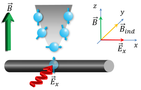
Figure 1: (Color online) The electron moving in a one-dimensional nanowire is constrained in a harmonic trap. The electron spin is initially polarized along the $z$-axis by an external static magnetic field $\vec{B}$. When an a.c. electric field $\vec{E}_{x}$ is applied to drive the electron, the electron spin will experience an additional magnetic field induced by the SOC. In our case, the magnetic field induced by Rashba SOC is perpendicular to the electric field.

In the next section, we present our model and show the origin of the effective magnetic field in EDSR. In Sec. III, the effective spin precession under the electric field through SOC is presented. We investigate how to speed up the coherent spin control with EDSR in Sec. IV. In Sec. V, we study the coherent spin control via EDSR in 2D QD system. Finally, the summary of our main results is given in Sec. VI. Some detailed calculations are displayed in the Appendices.

II the electric-dipole spin resonance

We first take the 1D nanowire QD system, where an electron is confined in an 1D harmonic trap along the $x$-direction with frequency $\omega$ (Fig. 1), as an illustration to explore the physical mechanism of EDSR. The model Hamiltonian reads Hamiltonian_1 ; Hamiltonian_2 ,

$$H=\hbar\omega a^{\dagger}a-i\tilde{\alpha}(a^{\dagger}-a)\sigma_{y}+\frac{1}{2}\hbar\omega_{z}\sigma_{z}+\xi(a^{\dagger}+a)\cos\nu t,$$ (1)

where $a=\sqrt{m_{e}\omega/(2\hbar)}[x+ip_{x}/(m_{e}\omega)]$ is the annihilation operator of the vibration degree of the electron with coordinate (momentum) $x\ (p_{x})$ and effective mass $m_{e}$, $\tilde{\alpha}=\alpha\sqrt{m_{e}\omega/(2\hbar)}$ with the Rashba SOC constant $\alpha$, $\xi=eE_{x}\sqrt{\hbar/(2m_{e}\omega)}$ is the effective driven strength of the a.c. electric field $-E_{x}\cos\nu t$. An external static magnetic field with strength $B$ is applied along the $z$-direction to to polarized the electronic spin. Here, $\omega_{z}=g\mu_{B}B/\hbar$ is the Zeeman splitting of the electron spin with the Bohr magneton $\mu_{B}$ and the effective $g$-factor $g$. Here, we just take the Rashba SOC into account, because our approach can be generalized to Dresselhaus case straightforwardly. Hereafter, we take $\hbar=1$ for convenience.

Now, we consider the dynamics of spin precession in a reference frame exactly following the classical trajectory of the driven electron in a harmonic trap. To this end, we introduce the time-dependent displacement transformation Cadez

$$D[f(t)]=e^{f(t)a^{\dagger}-{\rm h.c.}}\equiv e^{-i[p_{x}x_{c}(t)+xp_{c}(t)]},$$ (2)

where $p_{c}(t)=m\dot{x}_{c}$ and

$$x_{c}(t)=-\sqrt{\frac{2}{m_{e}\omega}}\frac{\omega\xi}{\omega^{2}-\nu^{2}}\cos\nu t,$$

corresponds to the classical trajectory of a driven harmonic oscillator (DHO) described by the classical Hamiltonian $\mathcal{H}_{c}=p_{c}^{2}/(2m_{e})+m\omega^{2}x_{c}^{2}/2+\sqrt{2m_{e}\omega}\xi x_{c}\cos\nu t$ (please refer to Appendix A for details). Here, $f(t)=-(\sqrt{m_{e}\omega/2}x_{c}+ip_{c}/\sqrt{2m_{e}\omega})$ represents a complex displacement in the phase space. As displayed in Appendix A, the above unitary transformation $D(t)=D[f(t)]$ is equivalent to the quantum linear coordinate transformation Leblond

$$x^{\prime}=x-x_{c}(t),\ t^{\prime}=t,\ \nabla^{\prime}=\nabla,\ \frac{\partial}{\partial t^{\prime}}=\frac{\partial}{\partial t}+\dot{x}_{c}\nabla^{\prime},$$ (3)

accompanied by a corresponding transformation of the wave function $\psi^{\prime}(x^{\prime},t^{\prime})=\psi(x,t)\rm{exp}(-i\phi)$, with $\phi=[p_{c}x^{\prime}+(1/m_{e})\int_{0}^{t^{\prime}}p_{c}^{2}(\tau)d\tau]$, as the requirement of covariance. The above transformation $D[f(t)]$ gives the equivalent Hamiltonian $H_{D}=DHD^{\dagger}-iD\left(\partial_{t}D^{\dagger}\right)$ in the reference frame moving along the classical path $x_{c}(t)$ as

$$H_{D} \!\!=\!\! \omega a^{\dagger}a\!-\!i\tilde{\alpha}(a^{\dagger}\!-\!a)\sigma_{y}\!-\!\eta\tilde{\alpha}\sigma_{y}\sin\nu t\!+\!\frac{1}{2}\omega_{z}\sigma_{z}.$$ (4)

Here, $\eta=2\nu\xi/(\omega^{2}-\nu^{2})$ is a dimensionless parameter and we have neglected a time-dependent c-number $\mathcal{E}_{c}=-(\omega\xi^{2}\cos^{2}\nu t)/(\omega^{2}-\nu^{2})$, which corresponds to the classical energy of this DHO.

It is found that $\eta$ is proportional to the driving strength $\xi$ and will be greatly enhanced if the driving frequency $\nu$ is nearly resonant with the frequency of the trap $\omega$. It follows Hamiltonian (4) that, in the new reference frame, a time-dependent spin flipping term appears, and its frequency is the same as the a.c. electric field.

III effective spin precession.

In experiment EDSR_E1D , the electron is tightly constrained in the trap with orbital transition energy $\sim 5-9{\rm meV}$ (corresponding oscillating frequency $\omega\sim 10^{12}-10^{13}{\rm Hz}$), the SOC strength $\tilde{\alpha}\sim 10^{9}{\rm Hz}$, the Zeeman splitting $\omega_{z}$ is of $\sim 10^{10}{\rm Hz}$ with $B\sim 100{\rm mT}$ and $g\approx 9$, and the driving frequency $\nu$ is resonant with $\omega_{z}$. Thus we have the condition $\omega\gg\omega_{z}\approx\nu>\tilde{\alpha}$, and then we can adiabatically eliminate the degree of the freedom of the vibration part to obtain the effective spin Hamiltonian.

The formal solution of the Heisenberg equation of $a(t)$ reads

$$a(t)=a(0)e^{-i\omega t}-\tilde{\alpha}e^{-i\omega t}\int_{0}^{t}\sigma_{y}(\tau)e^{i\omega\tau}d\tau.$$ (5)

In the case of $\omega\gg\omega_{z}\approx\nu>\tilde{\alpha}$, the oscillating frequency of the spin operator is of the scale $\sim\exp(\pm i\omega_{z}t)$, then the magnitude of the integral in Eq. (5) is approximated as $\tilde{\alpha}/(\omega\pm\omega_{z})\ll 1$. As a result, the influence of the SOC to the dynamics of the vibration part can be neglected. Then we can take the semi-classical approximation by replacing $a$ and $a^{\dagger}$ in Hamiltonian (4) with $\langle a(0)\rangle_{D}\exp(-i\omega t)$ and $\langle a^{\dagger}(0)\rangle_{D}\exp(i\omega t)$ ($\langle\cdots\rangle_{D}$ means averaging over the displaced initial state), respectively. For simplicity, we assume the system is in the state $\left|\psi(0)\right\rangle=\left|0\right\rangle\otimes\left|\uparrow\right\rangle$, and then the effective Hamiltonian for the spin part reads

$$H_{s}^{{\rm eff}}=\frac{1}{2}\omega_{z}\sigma_{z}-\eta\tilde{\alpha}\sigma_{y}\sin\nu t+\frac{2\omega}{\nu}\eta\tilde{\alpha}\sigma_{y}\sin\omega t.$$ (6)

Then the influences of the forced oscillation under the electric field and the free oscillation of the electron to the spin are described by two effective a.c. magnetic fields $B_{{\rm E}}=-B_{{\rm ind}}\sin\nu t$ and $B_{{\rm free}}=(2\omega/\nu)B_{{\rm ind}}\sin\omega t$, with $B_{{\rm ind}}=\eta\tilde{\alpha}/(g\mu_{B})$. The strengths of these two effective magnetic fields are both proportional to $\tilde{\alpha}\xi$. In 1D case, the effective magnetic fields induced by Rashba SOC (both $B_{{\rm free}}$ and $B_{{\rm E}}$) are perpendicular to the electric field, and the magnetic fields induced by the Dresselhaus SOC are parallel to the electric field.

We find that the effective magnetic field $B_{{\rm E}}$ generated by the forced oscillation of the electron under the electric field through SOC has the same frequency $\nu$ as the electric field. The effective field $B_{{\rm free}}$ generated by the free oscillation of the electron has the same frequency as the frequency of the harmonic trap $\omega$. Although the strength of $B_{{\rm free}}$ is $2\omega/\nu$ times lager than $B_{{\rm E}}$, it contribute little to the spin control, because its frequency $\omega$ is largely detuning from $\omega_{z}$. Therefore, in the case of $\omega\gg\omega_{z}\approx\nu>\tilde{\alpha}$, the dynamics of the spin can be described by the following Hamiltonian,

$$H_{s}^{{\rm RWA}}=\frac{1}{2}\omega_{z}\sigma_{z}-\frac{\eta\tilde{\alpha}}{2}(\sigma_{+}e^{-i\nu t}+\sigma_{-}e^{i\nu t}).$$ (7)

Here, we have neglected the influence of the fast oscillating term $B_{{\rm free}}$ and taken the rotating approximation (RWA) of the resonant term associated with $B_{{\rm E}}$.

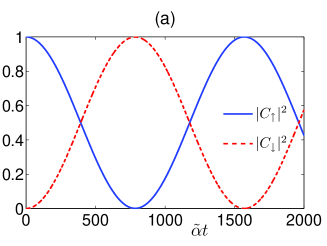
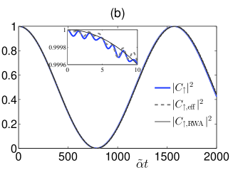
Figure 2: (Color online) We take the SOC constant as the unit $\tilde{\alpha}=1$. $\omega=250$, $\omega_{z}=2.5$, $\nu=2.5$, and $\xi=50$. (a) The solid blue (dashed red) line is the probability of the $\left|\uparrow\right\rangle$ ($\left|\downarrow\right\rangle$) state of the spin, which is directly calculated via $H_{D}$. (b) Probabilities of the spin state $\left|\uparrow\right\rangle$ obtained by different methods are presented. Solid blue line is obtained the numerical calculation via $H_{D}$. The dashed gray line is obtained from $H_{s}^{{\rm eff}}$. And the thin black line is obtained from $H_{s}^{{\rm RWA}}$ with rotating wave approximation.

To demonstrate the coherent control of the electron spin, we turn to numerical calculations. The spin is initially polarized in the state $\left|\uparrow\right\rangle$ and its wave function at time $t$ can be expanded as $\left|\chi(t)\right\rangle=C_{\uparrow}(t)\left|\uparrow\right\rangle+C_{\downarrow}(t)\left|\downarrow\right\rangle$. Here, $|C_{\uparrow}(t)|^{2}$ ($|C_{\downarrow}(t)|^{2}$) denotes the occupation probability of the state $\left|\uparrow\right\rangle$ ($\left|\downarrow\right\rangle$). In the case of $\omega\gg\omega_{z}=\nu>\tilde{\alpha}$, the perfect Rabi oscillation of the spin with frequency $\eta\tilde{\alpha}\sim(10^{-4}-10^{-3})\tilde{\alpha}$ is observed when the driving frequency $\nu$ is resonant with $\omega_{z}$ as shown in Fig. 2 (a). In Fig. 2 (b), the solid blue line is obtained directly from the Hamiltonian $H_{M}$ by tracing off the degree of freedom of the vibration, the dashed gray line is obtained from $H_{s}^{{\rm eff}}$, and thin black line is from $H_{s}^{{\rm RWA}}$. These three lines coincide with each other very well, except for some high-frequency fluctuation around the thin black line (obtained from $H_{s}^{{\rm RWA}}$) as shown in the subgraph of Fig. 2 (b). Thus, the dynamics of the spin is well described by $H_{s}^{{\rm RWA}}$ in the regime $\omega\gg\omega_{z}=\nu>\tilde{\alpha}$. And then the electron spin could be well controlled with electric field via EDSR as the same as ESR.

IV coherent-spin-control speed enhancement

In the preceding sections, we find that one can coherent control the electric spin with electric field through EDSR just like with magnetic field. Next, we will explore how to speed up coherent spin control with EDSR. First, we gives the condition to realize coherent control of electron spin with EDSR. For a spin-$1/2$ system described by Hamiltonian (7), the flipping probability $|C_{\downarrow}(t)|^{2}$ for the Rabi oscillation reads

$$|C_{\downarrow}(t)|^{2}=\frac{(\eta\tilde{\alpha})^{2}}{\delta^{2}+(\eta\tilde{\alpha})^{2}}\sin^{2}\left(\sqrt{\delta^{2}+(\eta\tilde{\alpha})^{2}}t/2\right),$$ (8)

where $\delta=\omega_{z}-\nu$ is the detuning between the driven frequency and the Zeeman splitting of the electron spin. As shown in Fig. 3 (a), the amplitude of the Rabi oscillation tends to $1$ when $\delta\ll\eta\tilde{\alpha}$, while the amplitude tends to $0$ when $\delta\gg\eta\tilde{\alpha}$. As a result, the flipping probability is deeply suppressed by the detuning $\delta$.

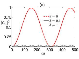
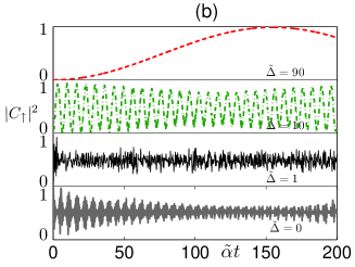
Figure 3: (Color online) Here, we take the SOC strength as the unit $\alpha=1$. (a) The flipping probabilities for different detunings $\delta$ between the driving electric field and the Zeeman splitting of the electron spin are presented. The parameters are taken as $\omega=100$, $\omega_{z}=10$, $\xi=10$. The dotted red line described the resonant case with $\nu=\omega_{z}$, $\delta=0$ and $\eta=0.0202$. The solid gray line described the case with $\nu=9.9$, $\delta=0.1$ and $\eta=0.02$. The thin black line described the large detuning case with $\nu=9$, $\delta=1$ and $\eta=0.0181$. (b) The flipping probabilities for different detunings $\tilde{\Delta}$ between frequency of the harmonic well and the Zeeman splitting of the electron spin are presented. Here, $\omega=100$, $\xi=10$, and the resonance condition $\delta=0$ is always guaranteed. And the other parameters are: $\nu=\omega_{z}=10$ with $\tilde{\Delta}=90$ for dotted red line, $\nu=\omega_{z}=90$ with $\tilde{\Delta}=10$ for dash-dotted green line, $\nu=\omega_{z}=99$ with $\tilde{\Delta}=1$ for thin black line, $\nu=\omega_{z}=100$ with $\tilde{\Delta}=0$ for solid gray line.

Similarly, when the detuning between the frequencies of harmonic trap and the Zeeman splitting $\tilde{\Delta}=\omega-\omega_{z}\gg\omega\eta\tilde{\alpha}/\nu$ is large, the effective magnetic field $B_{{\rm free}}$ hardly affect the spin-flipping process. As a result, the influence of the free oscillation of the electron to the dynamics of the spin can be neglected in the former section.

Starting from the original Hamiltonian (1), we numerically study the the influence of the detuning $\tilde{\Delta}$ to the coherent controlling of the spin. It is discovered that when $\tilde{\Delta}\gg\tilde{\alpha}$ and $\delta\ll\eta\tilde{\alpha}$, the coherent controlling of electron spin is realized as shown by the dotted red line ($\tilde{\Delta}=90\tilde{\alpha}$) and dashed-dot green line ($\tilde{\Delta}=10\tilde{\alpha}$) in Fig. 3 (b). When $\tilde{\Delta}\lesssim\tilde{\alpha}$, the SOC will destroy the coherence of the spin, and then collapse and revival phenomenon appear. As shown by the thin black line ($\tilde{\Delta}=1\tilde{\alpha}$) and solid gray line $\tilde{\Delta}=0$ in Fig. 4, the coherent controlling of the electron spin is destroyed by SOC. As a result, to realize a perfect spin control through EDSR, two necessary conditions must be guaranteed: (1) the frequency of the a.c. electric field must be resonant with the Zeeman splitting of the spin in the external magnetic field, i.e., $\delta\ll\eta\tilde{\alpha}$; (2) the frequency of the harmonic trap must be largely detuned from the Zeeman splitting of the spin, i.e., $|\tilde{\alpha}/\tilde{\Delta}|\ll 1$.

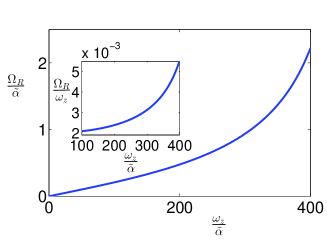
Figure 4: (Color online) Here, we take the SOC strength as the unit $\alpha=1$. The Rabi frequency of the coherence spin flip increases with $\omega_{z}$. The parameters are taken as $\xi=\omega=500$.

According to Eq. (8), spin-flip speed is charaterized by the Rabi frequency:

$$\Omega_{R}=\frac{1}{2}\eta\tilde{\alpha}=\frac{\omega_{z}\xi\tilde{\alpha}}{\omega^{2}-\omega_{z}^{2}},$$ (9)

where we have used the resonance condition $\delta=\omega_{z}-\nu=0$. It is found that this Rabi frequency $\Omega_{R}$ is proportional to the strengths of the SOC $\tilde{\alpha}$ and electric driving $\xi$. Hence, we should increase $\tilde{\alpha}$ and $\xi$ to enlarge $\Omega_{R}$. But if the driving strength $\xi\gg\omega$, the electron will flee from the harmonic trap. When $\tilde{\alpha}$ is large enough to break the large detuning condition $|\tilde{\alpha}/\tilde{\Delta}|\ll 1$, the free oscillation of the electron and the spin precession will be highly correlated, thus the SOC will destroy the coherent control according to Hamiltonian (4). For safety, we require $\xi\leqslant\omega$ and $0<\tilde{\alpha}/\tilde{\Delta}\leqslant 0.01$ to guarantee the perfect Rabi oscillation of the electron spin in the trap. From Eq. (9), $\Omega_{R}$ monotonically increases with $\omega_{z}$ with upper limit $10^{-2}\omega_{z}$ for this case (see Fig. 4). Thus, for a very large $\omega$, one can increase $\omega_{z}$, besides the driving strength $\xi$ and SOC strength $\tilde{\alpha}$, to speed up the spin flipping.

V two-dimensional Quantum Dot system

For the two-dimensional (2D) QD system, the magnetic field induced by the a.c. electric field via SOC becomes much more complicated and azimuth-dependent. We can utilize this azimuth dependence to measure the Rashba and Dresselhaus SOC strength ratio and realize a perfect single electron spin qubit operation through EDSR.

The Hamiltonian of the electron confined in an 2D harmonic well $H=H_{v}+H_{s}+H_{{\rm so}}+V(t)$ is composed of four parts: the vibration part of the electron is described with

$$H_{v}=\frac{1}{2m_{e}}[\vec{p}+\frac{e}{c}\vec{A}(\vec{r})]^{2}+\frac{1}{2}m_{e}\tilde{\omega}_{x}^{2}x^{2}+\frac{1}{2}m_{e}\tilde{\omega}_{y}^{2}y^{2},$$ (10)

where $\vec{p}=p_{x}\vec{e}_{x}+p_{y}\vec{e}_{y}$ is the in-plane momentum, $\tilde{\omega}_{x(y)}$ the frequency of the harmonic trap of $x(y)$-direction, and $\vec{A}(\vec{r})=B(0,0,y\cos\varphi_{B}-x\sin\varphi_{B})$ the vector potential for the in-plane static magnetic field $\vec{B}=B(\cos\varphi_{B},\sin\varphi_{B},0)$. The second part $H_{s}=\hbar g\mu_{B}\vec{B}\cdot\vec{\sigma}/2$ describes the Zeeman splitting of the electron spin in $\vec{B}=B(\cos\varphi_{B},\sin\varphi_{B},0)$. For the third part, both the Rashba and Dresselhaus SOC with strength $\alpha_{R}$ and $\alpha_{D}$ respectively are taken into account

$$H_{{\rm so}}=\alpha_{R}(\sigma_{x}p_{y}-\sigma_{y}p_{x})+\alpha_{D}(\sigma_{y}p_{y}-\sigma_{x}p_{x}).$$ (11)

The last part $V(t)=-e\vec{r}\cdot\vec{E}(t)$ describes the driven of the electron under an in-plane a.c. electric field $\vec{E}(t)=-\left(E\vec{e}_{x}\cos\varphi_{E}+E\vec{e}_{y}\sin\varphi_{E}\right)\cos\nu t$.

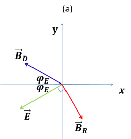
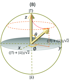
Figure 5: (Color online) The 2D electric field caused spin precession on the Bloch sphere. (a) The a.c. magnetic field induced by Dresselhaus SOC and the a.c. electric field lie at two different sides of the $x$-axis with the same angle from the $x$-axis. The magnetic field induced by Rashba SOC $\vec{B}_{R}$ is always vertical to $\vec{E}$. (b) The trajectory of the spin from the initial point $\rho(0)=\left|\uparrow\right\rangle\left\langle\uparrow\right|$ to the final state $\rho(\theta,\phi)$ with $\theta=g\mu_{B}B_{R}t/2$ and $\phi=\nu t+\varphi_{E}$ on the Bloch sphere surface.

After a similar unitary transformation as the 1D case, the a.c. electric field will be converted to an a.c. magnetic field with the same frequency (please refer to Appendix B for details). In the experiment EDSR_E2D , the external static magnetic field is week, i.e., the frequency modification induced by the vector potential can be neglected $\omega_{c}=eB/(m_{e}c)\ll\tilde{\omega}_{x(y)}$ NZhao . In this case, the effective spin Hamiltonian for the isotropic 2D harmonic well $\tilde{\omega}_{x}=\tilde{\omega}_{y}=\omega$ could be simplified to

$$H_{s}^{{\rm eff}}=\frac{1}{2}g\mu_{B}\left[\vec{B}+\vec{B}_{R}(t)+\vec{B}_{D}(t)\right]\cdot\vec{\sigma},$$ (12)

where $\vec{B}_{R}(t)=B_{R}\sin\nu t(\sin\varphi_{E},-\cos\varphi_{E},0)$ and $\vec{B}_{D}(t)=B_{D}\sin\nu t(-\cos\varphi_{E},\sin\varphi_{E},0)$ are the magnetic fields induced by Rashba and Dresselhaus SOC respectively, with strength

$$B_{R(D)}(t)=\frac{2\hbar\nu eE\alpha_{R(D)}}{g\mu_{B}\left(\omega^{2}-\nu^{2}\right)}.$$ (13)

It is observable that $\vec{B}_{R}$ is always vertical to the electric field $\vec{E}$, but $\vec{B}_{D}$ is vertical to $\vec{E}$ only when $\varphi_{E}=n\pi/2+\pi/4\ (n=0,1,2,3)$ [see Fig. 5 (a)]. When $\varphi_{E}=3\pi/4\ {\rm or}\ 7\pi/4$, $\vec{B}_{R}$ and $\vec{B}_{D}$ are parallel, while $\vec{B}_{R}$ and $\vec{B}_{D}$ are anti-parallel when $\varphi_{E}=\pi/4\ {\rm or}\ 5\pi/4$. Therefore, one can measure the ratio of the SOC strength $\alpha_{R}/\alpha_{D}$ by measuring the different Rabi frequencies for $\varphi_{E}=\pi/4$ and $\varphi_{E}=3\pi/4$ EDSR_T0 .

In addition, the direction of the effective magnetic field can be well controlled by tuning the direction fo the a.c. electronic field. For the case where the static magnetic field along $z$-direction $\vec{B}=B(0,0,1)$ instead of the in-plane one is applied, the induced magnetic fields are nearly the same. If there is only one type of SOC (e.g., Rashba one), we can use the electric field to induce an effective magnetic field in any needed direction, which controls the evolution of the spin state from a starting point to anywhere we wanted on the Bloch sphere. If the electric field is resonant with the Zeeman splitting of the spin (i.e., $\nu=g\mu_{B}B$, the dynamics of the spin can be described by the Hamiltonian

$$H_{s}^{RWA}\!=\!\frac{g\mu_{B}}{2}{B\sigma_{z}\!-\!\frac{B_{R}}{2}[e^{-i(\varphi_{E}+\nu t)}\sigma_{+}\!+\!e^{i(\varphi_{E}+\nu t)}\sigma_{-}]}.$$ (14)

An arbitrary target state $\rho(\theta,\phi)=(1+\vec{n}\cdot\vec{\sigma})/2$ with $\vec{n}=(\sin\theta\cos\phi,\sin\theta\sin\phi,\cos\theta)$ on the Bloch sphere can be realized through EDSR by choosing proper time $g\mu_{B}B_{R}t/2=\theta$ and proper angle $\varphi_{E}=\phi-\nu t$ from the starting point $\rho_{0}=\left|\uparrow\right\rangle\left\langle\uparrow\right|$ [see Fig. 5 (b)]. Namely, the electric field can perform a perfect single-qubit operation in the spin system through EDSR.

VI summary

For the physical mechanism of EDSR in 1D nanowire QD or for 2D case, we provide an intuitive explanation with an exact picture in physics based on the reference frame transformation: the electric field can behaves as magnetic field in the reference frame exactly following the classical trajectory of a DHO. This electric-magnetic duality can be generally found in relativistic transformation of the Maxwell equations. We also notice that SOC is in essence the consequence of relativistic quantum theory in the low-velocity limit. Thus our approach presented in this letter is, in principle, consistent with the point of view of special relativity.

For the EDSR technology itself, our study shows that two necessary conditions must be guaranteed to realize a perfect spin control through EDSR:(1) the frequency of the a.c. electric field must be resonant with the Zeeman splitting of the spin; (2)the detuning beween the frequency of the harmonic trap and the Zeeman splitting of the spin must be much larger than SOC coupling strength. Based on these conditions, there are three ways to increase the speed of coherent spin control: (1) increasing the electric driving strength;(2) increasing the strength of SOC $\tilde{\alpha}$; (3) increaseing the external state magnetic field to increase the Zeeman splitting of the electron spin.

The azimuthal dependence of the induced magnetic field can be used to measure the ratio of the strengths of the Rashba and Dresselhaus SOC. We also shown that the precise control of spin in the whole Bloch sphere can be realized in 2D QD system through EDSR technology.

We thank Da-Zhi Xu and Prof. Xia-Ji Liu for helpful discussion. This work was supported by the National Natural Science Foundation of China Grant No.11121403 and the National 973 program (Grant No. 2012CB922104 and No. 2014CB921403).

Appendix A the quantum driven harmonic oscillator

A.1 Time-dependent displacement transformation

The exact solution of the Schrödinger equation of a quantum driven harmonic oscillator (DHO) described by Hamiltonian

$$H=\omega a^{\dagger}a+[F(t)a+{\rm h.c.}],$$ (15)

has given by Husimi Husimi in 1953 (and independently by Kerner Kerner in 1958). Here, we give another method to deal this problem by taking a time-dependent displacement transformation

$$D[f(t)]=\exp[f(t)a^{\dagger}-f^{*}(t)a],$$ (16)

where function $f(t)$ is to be determined. It is ready to find the relations

$$DaD^{\dagger}=a-f(t),\ {\rm and}\ Da^{\dagger}D^{\dagger}=a^{\dagger}-f^{*}(t).$$ (17)

After the transformation, the effective Hamiltonian reads

$$\tilde{H} = DHD^{\dagger}-iD\left(\frac{\partial}{\partial t}D^{\dagger}\right)$$ (19)

$$= \omega a^{\dagger}a-(\omega f-F^{*}-i\dot{f})a^{\dagger}-(\omega f^{*}-F+i\dot{f}^{*})a$$

$$+\omega|f|^{2}-(Ff+F^{*}f^{*})+\frac{i}{2}(f\dot{f}^{*}-\dot{f}f^{*}).$$

One finds that the Hamiltonian will be diagonalized if we choose suitable function $f(t)$ satisfying

$$\omega f-F^{*}-i\dot{f} = 0,$$ (20a)

$$\omega f^{*}-F+i\dot{f}^{*} = 0.$$ (20b)

Now we split $f(t)$ into real and imaginary parts

$$f(t)=-\left(\sqrt{\frac{m_{e}\omega}{2}}x_{c}+i\sqrt{\frac{1}{2m_{e}\omega}}p_{c}\right).$$ (21)

Then Eqs. (20a) and (20b) change into

$$\dot{p}_{c} = -\left[m\omega^{2}x_{c}+\sqrt{\frac{m_{e}\omega}{2}}(F+F^{*})\right],$$ (22a)

$$\dot{x}_{c} = \frac{p_{c}}{m}+i\sqrt{\frac{1}{2m_{e}\omega}}(F-F^{*}).$$ (22b)

If $F$ is real, it is observable that $x_{c}$ and $p_{c}$ satisfy the classical Hamilton equation generating by the classical Hamiltonian of a forced classical harmonic oscillator

$$\mathcal{H}_{c}=\frac{p_{c}^{2}}{2m_{e}}+\frac{1}{2}m_{e}\omega^{2}x_{c}^{2}+\tilde{F}(t)x_{c},$$ (23)

with $\tilde{F}(t)=\sqrt{2m_{e}\omega}F(t)$.

In our case $F=F^{*}=\xi\cos\nu t$, then we obtain the solution

$$\!\!\!\!\!\!\!\!\!\!\!x_{c}(t)\!\! =\!\! \!-\sqrt{\!\!\frac{2}{m_{e}\omega}}\!\frac{\omega\xi}{\omega^{2}\!-\!\nu^{2}}\!\cos\nu t\!+\!A\sin\omega t\!+\!B\cos\omega t\!,$$ (24)

$$\!\!\!\!\!\!\!\!\!\!\!p_{c}(t)\!\! =\!\! \!\!\sqrt{2m_{e}\omega}\!\frac{\nu\xi}{\omega^{2}\!-\!\nu^{2}}\!\sin\nu t\!+\!A\omega\!\cos\omega t\!-\!B\omega\!\sin\omega t\!,$$ (25)

where $A$ and $B$ are time-independent constants. For simplicity, we take $A=B=0$ (corresponding to the special initial conditions $x_{c}(0)=-\sqrt{2\omega/m_{e}}\xi/(\omega^{2}-\nu^{2})$ and $\dot{x}_{c}(0)=0$), then the displacement operator reads

$$D=e^{-i[px_{c}(t)+xp_{c}(t)]},$$ (26)

and the Hamiltonian changes into

$$H_{D}=\omega a^{\dagger}a+\mathcal{E}_{c},$$ (27)

where

$$\mathcal{E}_{c}=-\frac{\omega\xi^{2}}{\omega^{2}-\nu^{2}}\cos^{2}\nu t.$$ (28)

As shown in the following subsection, $\mathcal{E}_{c}$ corresponds to the classical energy for the DHO.

A.2 Equivalent quantum linear coordinate transformation

In this subsection, it will shown that the time-dependent unitary transformation in the former subsection corresponds to a quantum linear coordinate transformationRosen ; Husimi .

Now, we rewrite the Hamiltonian of the DHO as

$$H = -\frac{\hbar^{2}}{2m_{e}}\nabla^{2}+\frac{1}{2}m_{e}\omega^{2}x^{2}+\tilde{F}(t)x.$$ (29)

Then we take a linear coordinate-translation transformation

$$x^{\prime}=x-x_{c}(t),$$ (30)

where the time-dependent c-number $x_{c}(t)$ satisfies the classical Hamilton equation

$$\dot{x}_{c} = \frac{p_{c}}{m_{e}},$$ (31a)

$$\dot{p}_{c} = -m_{e}\omega^{2}x_{c}-\tilde{F}(t),$$ (31b)

i.e.,

$$m_{e}\ddot{x}_{c}+m_{e}\omega^{2}x_{c}+\tilde{F}(t)=0.$$ (32)

Obviously, $x_{c}(t)$ describes the classical path of the DHO. It is ready to obtain the following relations

$$x^{\prime}=x-x_{c}(t),\ t^{\prime}=t,\ \nabla^{\prime}=\nabla,\ \frac{\partial}{\partial t^{\prime}}=\frac{\partial}{\partial t}+\dot{x}_{c}\nabla^{\prime}.$$ (33)

As the consequence of the required covariance,

$$i\hbar\frac{\partial}{\partial t^{\prime}}\psi^{\prime}(x^{\prime},t^{\prime})=H^{\prime}\psi^{\prime}(x^{\prime},t^{\prime}),$$ (34)

a transformation of the wave function is needed

$$\psi^{\prime}(x^{\prime},t^{\prime})=\psi(x,t)e^{-i\phi},$$ (35)

with

$$\phi=\frac{1}{\hbar}\left[p_{c}x^{\prime}+\frac{1}{m_{e}}\int_{0}^{t^{\prime}}p_{c}^{2}(\tau)d\tau\right].$$ (36)

Here, the Hamiltonian in the new reference frame reads

$$H^{\prime} = -\frac{\hbar^{2}}{2m}\nabla^{\prime 2}+\frac{1}{2}m\omega^{2}x^{\prime 2}+\mathcal{H}_{c}(t),$$ (37)

where

$$\mathcal{H}_{c}(t) = \frac{p_{c}^{2}}{2m_{e}}+\frac{1}{2}m_{e}\omega^{2}x_{c}^{2}+\tilde{F}(t^{\prime})x_{c},$$ (38)

is the classical Hamiltonian of the DHO. It is found that the DHO moves as a free harmonic oscillator in this new reference frame.

For our case $F=\hbar\xi\cos\nu t$, we also take the solution of the Hamilton equation (32) as

$$x_{c}(t)=-\sqrt{\frac{2\omega}{\hbar m_{e}}}\frac{\xi\cos\nu t^{\prime}}{\omega^{2}-\nu^{2}}.$$ (39)

Following Eq. (38), we obtain the classical energy of the DHO

$$\mathcal{E}_{c}(t^{\prime})=-\frac{\omega\xi^{2}}{\omega^{2}-\nu^{2}}\cos^{2}\nu t^{\prime},$$ (40)

which is the exact time-dependent function defined in Eq. (28). Here, we have neglected a time-independent constant $\omega\xi^{2}\nu^{2}/(\omega^{2}-\nu^{2})^{2}$ and taken $\hbar=1$. Consequently, this quantum linear coordinate transformation is equivalent with the time-dependent displacement $D(t)$ defined in Eq. (16).

Appendix B effective spin precession in two-dimensional quantum dot system

B.1 Diagonalization of the vibration potential

By defining creation and annihilation operators

$$x=\frac{1}{\sqrt{2m_{e}\omega_{x}}}(a^{\dagger}+a),\ p_{x}=i\sqrt{\frac{m_{e}\omega_{x}}{2}}(a^{\dagger}-a),$$ (41)

$$y=\frac{1}{\sqrt{2m_{e}\omega_{y}}}(b^{\dagger}+b),\ p_{y}=i\sqrt{\frac{m_{e}\omega_{y}}{2}}(b^{\dagger}-b),$$ (42)

we rewrite the vibration Hamiltonian (10) of the electron in 2D QD system as

$$H_{v} = \omega_{x}a^{\dagger}a+\omega_{y}b^{\dagger}b-\chi(a^{\dagger}b+ab^{\dagger})$$

where

$$\omega_{x}^{2} = \tilde{\omega}_{x}^{2}+\omega_{c}^{2}\sin^{2}\varphi_{B},$$ (43)

$$\omega_{y}^{2} = \tilde{\omega}_{y}^{2}+\omega_{c}^{2}\cos^{2}\varphi_{B},$$ (44)

$$\omega_{c} = \frac{eB}{m_{e}c}.$$ (45)

and we have taken the rotating wave approximation since

$$\chi=\omega_{c}\sin 2\varphi_{B}\sqrt{\frac{\omega_{c}^{2}}{\omega_{x}\omega_{y}}}\ll\omega_{x(y)}.$$ (46)

And the SOC Hamiltonian $H_{{\rm so}}$ and the driven part $V(t)$ change into

$$H_{{\rm so}} = i\sqrt{\frac{m_{e}\omega_{y}}{2}}(\alpha_{R}\sigma_{x}+\alpha_{D}\sigma_{y})(b^{\dagger}-b)$$ (47)

$$-i\sqrt{\frac{m_{e}\omega_{x}}{2}}(\alpha_{R}\sigma_{y}+\alpha_{D}\sigma_{x})(a^{\dagger}-a),$$

and

$$V(t)=eE\left[\sqrt{\frac{1}{2m_{e}\omega_{x}}}(a^{\dagger}+a)\cos\varphi_{E}+\sqrt{\frac{1}{2m_{e}\omega_{y}}}(b^{\dagger}+b)\sin\varphi_{E}\right]\cos\nu t,$$ (48)

respectively. Hereafter, we let $\hbar=1$ for simplicity.

It is convenient to diagonalize $H_{v}$ by defining two new modes,

$$\left(\begin{array}[]{c}A\\ B\end{array}\right)=\left(\begin{array}[]{cc}\cos\frac{\vartheta}{2}&-\sin\frac{\vartheta}{2}\\ \sin\frac{\vartheta}{2}&\cos\frac{\vartheta}{2}\end{array}\right)\left(\begin{array}[]{c}a\\ b\end{array}\right),$$ (49)

where

$$\cos\vartheta=\frac{\Delta/2}{\sqrt{\Delta^{2}/4+\chi^{2}}},\ \sin\vartheta=\frac{\chi}{\sqrt{\Delta^{2}/4+\chi^{2}}},$$ (50)

and $\Delta=\omega_{x}-\omega_{y}$. Then the total Hamiltonian of the 2D QD system $H=H_{v}+H_{s}+H_{{\rm so}}+V(t)$ changes into

$$H_{v}=\omega_{A}A^{\dagger}A+\omega_{B}B^{\dagger}B,$$ (51)

$$H_{s}=\frac{1}{2}g\mu_{B}\vec{B}\cdot\vec{\sigma},$$ (52)

$$\!\!\!\!\!\!V(t) = \!\xi_{A}(A^{\dagger}\!+\!A)\cos\nu t\!+\!\xi_{B}(B^{\dagger}+B)\cos\nu t,$$ (53)

and

$$H_{{\rm so}} = i\left[\sqrt{\frac{m_{e}\omega_{y}}{2}}(\alpha_{R}\sigma_{x}+\alpha_{D}\sigma_{y})\cos\frac{\vartheta}{2}-\sqrt{\frac{m_{e}\omega_{x}}{2}}(\alpha_{R}\sigma_{y}+\alpha_{D}\sigma_{x})\sin\frac{\vartheta}{2}\right](B^{\dagger}-B)$$ (54)

$$-i\left[\sqrt{\frac{m_{e}\omega_{y}}{2}}(\alpha_{R}\sigma_{x}+\alpha_{D}\sigma_{y})\sin\frac{\vartheta}{2}+\sqrt{\frac{m_{e}\omega_{x}}{2}}(\alpha_{R}\sigma_{y}+\alpha_{D}\sigma_{x})\cos\frac{\vartheta}{2}\right](A^{\dagger}-A).$$

Here, the frequencies of the new two modes are

$$\omega_{A} = \frac{\omega_{x}+\omega_{y}}{2}+\sqrt{\frac{\Delta^{2}}{4}+\chi^{2}},$$ (55)

$$\omega_{B} = \frac{\omega_{x}+\omega_{y}}{2}-\sqrt{\frac{\Delta^{2}}{4}+\chi^{2}},$$ (56)

and corresponding driving strength of the electric field,

$$\!\!\!\!\!\!\!\!\!\!\xi_{A}\!\! = \!\!\frac{eE}{\sqrt{2m_{e}}}\![\frac{1}{\sqrt{\omega_{x}}}\!\cos\frac{\vartheta}{2}\!\cos\varphi_{E}\!-\!\!\frac{1}{\sqrt{\omega_{y}}}\sin\frac{\vartheta}{2}\!\sin\varphi_{E}],$$ (57)

$$\!\!\!\!\!\!\!\!\!\!\xi_{B}\!\! = \!\!\frac{eE}{\sqrt{2m_{e}}}\![\frac{1}{\sqrt{\omega_{x}}}\!\sin\frac{\vartheta}{2}\!\cos\varphi_{E}\!+\!\frac{1}{\sqrt{\omega_{y}}}\cos\frac{\vartheta}{2}\!\sin\varphi_{E}].$$ (58)

B.2 Effective spin-controlling Hamiltonian

Just like the one-dimensional case, we take a similar unitary transformation

$$D[t] = \exp\left[f_{A}(t)A^{\dagger}+f_{B}(t)B^{\dagger})-{\rm h.c.}\right].$$ (59)

where

$$f_{A} = \frac{\xi_{A}}{\omega_{A}^{2}-\nu^{2}}(\omega\cos\nu t-i\nu\sin\nu t),$$ (60)

$$f_{B} = \frac{\xi_{B}}{\omega_{B}^{2}-\nu^{2}}(\omega\cos\nu t-i\nu\sin\nu t).$$ (61)

Then the Hamiltonian changes into $H=H_{v}+H_{s}+H_{{\rm so}}+H_{{\rm flip}}$, where

$$H_{v}=\omega_{A}A^{\dagger}A+\omega_{B}B^{\dagger}B,$$ (62)

and

$$\!\!\!\!\!\!\!\!\!\!\!\!\!\!H_{{\rm flip}}\!\!\! = \!\!\![G_{1}(\alpha_{R}\sigma_{x}\!+\!\alpha_{D}\sigma_{y})\!-\!G_{2}(\alpha_{R}\sigma_{y}\!+\!\alpha_{D}\sigma_{x})]\!\sin\nu t\!,$$ (63)

with

$$G_{1} = \frac{1}{2}\eta_{B}(\sqrt{\frac{\omega_{y}}{\omega_{x}}}\sin\frac{\vartheta}{2}\cos\frac{\vartheta}{2}\cos\varphi_{E}+\cos^{2}\frac{\vartheta}{2}\sin\varphi_{E})-\frac{1}{2}\eta_{A}(\sqrt{\frac{\omega_{y}}{\omega_{x}}}\sin\frac{\vartheta}{2}\cos\frac{\vartheta}{2}\cos\varphi_{E}+-\sin^{2}\frac{\vartheta}{2}\sin\varphi_{E}),$$ (64)

$$G_{2} = \frac{1}{2}\eta_{B}\left(\sqrt{\frac{\omega_{x}}{\omega_{y}}}\sin\frac{\vartheta}{2}\cos\frac{\vartheta}{2}\sin\varphi_{E}+\sin^{2}\frac{\vartheta}{2}\cos\varphi_{E}\right)-\frac{1}{2}\eta_{A}\left(\sqrt{\frac{\omega_{x}}{\omega_{y}}}\sin\frac{\vartheta}{2}\cos\frac{\vartheta}{2}\sin\varphi_{E}-\cos^{2}\frac{\vartheta}{2}\cos\varphi_{E}\right).$$ (65)

Here, the additional spin-flipping term $H_{{\rm flip}}$ is generated by the electric field mediated by SOC and

$$\eta_{A(B)}=\frac{2\nu eE}{\omega_{A(B)}^{2}-\nu^{2}}.$$ (66)

For most case, the azimuthal dependence of $H_{{\rm flip}}$ about $\varphi_{E}$ is complicate. In experiment, the external static magnetic field is week $\chi\ll\omega$, and then the influence of the vector potential $\vec{A}(\vec{r})$ can be neglected, i.e., $\vartheta\rightarrow 0$ and $\omega_{A(B)}\approx\tilde{\omega}_{x(y)}$. If the 2D harmonic well is isotropic $\tilde{\omega}_{x}=\tilde{\omega}_{y}=\omega$, $H_{{\rm flip}}$ will get highly simplified as

$$H_{{\rm flip}}=\frac{1}{2}g\mu_{B}\left[\vec{B}_{R}(t)+\vec{B}_{D}(t)\right]\cdot\vec{\sigma},$$

where $\vec{B}_{R}(t)=B_{R}\sin\nu t(\sin\varphi_{E},-\cos\varphi_{E},0)$ is magnetic fields induced by Rashba spin-orbit coupling and the magnetic field induced by Dresselhaus coupling is $\vec{B}_{D}(t)=B_{D}\sin\nu t(-\cos\varphi_{E},\sin\varphi_{E},0)$ with strengths

$$B_{R(D)}=\frac{2\nu eE\alpha_{R(D)}}{g\mu_{B}\left(\omega^{2}-\nu^{2}\right)}.$$ (67)

References

- (1) R. Hanson, L. P. Kouwenhoven, J. R. Petta, S. Tarucha, and L. M. K. Vandersypen, Rev. Mod. Phys. 79, 1217 (2007).
- (2) R. Hanson et al., Phys. Rev. Lett. 94, 196802 (2005).
- (3) Willems van Berveren, New J. Phys. 7,182 (2005).
- (4) J. Berezovsky, M. H. Mikkelsen, N. G. Stoltz, L. A. Coldren, D. D. Awschalom, Science 320, 349 (2008).
- (5) S. Nadj-Perge et al., Phys. Rev. B 81,201305 (2010).
- (6) S. Hermelin et al., Nature 477, 435 (2011).
- (7) R. P. G. McNeil et al., Nature 477, 439 (2011).
- (8) M. Kataoka et al., Phys. Rev. Lett. 106, 126801 (2011).
- (9) S. A. Wolf et al., Science 294, 1488 (2001).
- (10) D. Awschalom, D. Loss, and N. Samarth, Semiconductor Spintronics and Quantum Computation (Springer-Verlag, Berlin, 2002).
- (11) C. P. Poole, Electron Spin Resonance 2nd edn (Wiley, New York, 1983).
- (12) F.H. L. Koppens et al., nature 442, 766 (2006).
- (13) D. Press et al., Nature 456, 218 (2008).
- (14) E. I. Rashba and Al. L. Efros, Phys. Rev. Lett. 91, 126405 (2003).
- (15) E. I. Rashba and Al. L. Efros, Appl. Phys. Lett. 83, 5295 (2003).
- (16) G. Dresselhaus, Phys. Rev. 100, 580 (1955).
- (17) Y. A. Bychkov and E. I. Rashba, J. Phys. C 17, 6039 (1984).
- (18) K. C. Nowack et al., Science 318, 1430 (2007).
- (19) E. A. Laird et al., Phys. Rev. Lett. 99, 246601 (2007).
- (20) M. Pioro-Ladrière et al., Nat. Phys. 4, 776 (2008).
- (21) S. Nadj-Perge et al., Nature (London) 468, 1084 (2010); S. Nadj-Perge et al., Phy. Rev. Lett. 108, 166801 (2012).
- (22) M. Shafiei, K. C. Nowack, C. Reichl, W. Wegscheider, and L. M. K. Vandersypen, Phys. Rev. Lett. 110, 107601 (2013).
- (23) E. I. Rashba and V. I. Sheka, in Landau Level Spectroscopy (North-Holland, Amsterdam, 1991), p. 131.
- (24) Vitaly N. Golovach, Massoud Borhani, and Daniel Loss, Phys. Rev. B 74, 165319 (2006).
- (25) E. I. Rashba, Phys. Rev. B 78, 195302 (2008).
- (26) S. Bednarek, J. Pawlowski and A. Skubis, Appl. Phys. Lett. 100, 203103 (2012).
- (27) Rui Li, J. Q. You, C. P. Sun, and Franco Nori, Phys. Rev. Lett. 111, 086805 (2013).
- (28) Y. N. Fang, Yusuf Turek, J. Q. You, and C. P. Sun, arXiv:1308.5387.
- (29) D. V. Khomitsky, L. V. Gulyaev, and E. Y. Sherman., Phys. Rev. B 85, 125312 (2012).
- (30) Yuriy V. Pershin, James A. Nesteroff, and Vladimir Privman, Phys. Rev. B 69, 121306 (2004).
- (31) Christian Flindt, Anders S. Sørensen, and Karsten Flensberg, Phys. Rev. Lett. 97, 240501 (2006).
- (32) T. Čadež, J. H. Jefferson, and A. Ramšak, New Journal of Physics, 15, 013029 2013; arXiv:1312.7254.
- (33) J.-M. Levy-Leblond, Commun. Math. Phys. 6, 286 (1967); G. Rosen, Am. J. Phys. 40, 683 (1972).
- (34) Nan Zhao, L. Zhong, Jia-Lin Zhu, and C. P. Sun, Phys. Rev. B 74, 075307 (2006).
- (35) K. Husimi, Prog. Theo. Phys. 4, 381 (1953).
- (36) E. H. Kerner, Can. J. Phys. 36, 371 (1958).
- (37) G. Rosen, Am. J. Phys. 40, 683 (1972).