The D0 Collaboration111with visitors from
aAugustana College, Sioux Falls, SD, USA,
bThe University of Liverpool, Liverpool, UK,
cDESY, Hamburg, Germany,
dUniversidad Michoacana de San Nicolas de Hidalgo, Morelia, Mexico
eSLAC, Menlo Park, CA, USA,
fUniversity College London, London, UK,
gCentro de Investigacion en Computacion - IPN, Mexico City, Mexico,
hUniversidade Estadual Paulista, São Paulo, Brazil,
iKarlsruher Institut für Technologie (KIT) - Steinbuch Centre for Computing (SCC),
D-76128 Karlsrue, Germany,
jOffice of Science, U.S. Department of Energy, Washington, D.C. 20585, USA,
kAmerican Association for the Advancement of Science, Washington, D.C. 20005, USA
and
lKiev Institute for Nuclear Research, Kiev, Ukraine
Improved b quark jet identification at the D0 experiment
V.M. Abazov
Joint Institute for Nuclear Research, Dubna, Russia
B. Abbott
University of Oklahoma, Norman, Oklahoma 73019, USA
B.S. Acharya
Tata Institute of Fundamental Research, Mumbai, India
M. Adams
University of Illinois at Chicago, Chicago, Illinois 60607, USA
T. Adams
Florida State University, Tallahassee, Florida 32306, USA
J.P. Agnew
The University of Manchester, Manchester M13 9PL, United Kingdom
G.D. Alexeev
Joint Institute for Nuclear Research, Dubna, Russia
G. Alkhazov
Petersburg Nuclear Physics Institute, St. Petersburg, Russia
A. AltonaUniversity of Michigan, Ann Arbor, Michigan 48109, USA
A. Askew
Florida State University, Tallahassee, Florida 32306, USA
S. Atkins
Louisiana Tech University, Ruston, Louisiana 71272, USA
K. Augsten
Czech Technical University in Prague, Prague, Czech Republic
C. Avila
Universidad de los Andes, Bogotá, Colombia
F. Badaud
LPC, Université Blaise Pascal, CNRS/IN2P3, Clermont, France
L. Bagby
Fermi National Accelerator Laboratory, Batavia, Illinois 60510, USA
B. Baldin
Fermi National Accelerator Laboratory, Batavia, Illinois 60510, USA
D.V. Bandurin
University of Virginia, Charlottesville, Virginia 22904, USA
S. Banerjee
Tata Institute of Fundamental Research, Mumbai, India
E. Barberis
Northeastern University, Boston, Massachusetts 02115, USA
P. Baringer
University of Kansas, Lawrence, Kansas 66045, USA
J.F. Bartlett
Fermi National Accelerator Laboratory, Batavia, Illinois 60510, USA
U. Bassler
CEA, Irfu, SPP, Saclay, France
V. Bazterra
University of Illinois at Chicago, Chicago, Illinois 60607, USA
A. Bean
University of Kansas, Lawrence, Kansas 66045, USA
M. Begalli
Universidade do Estado do Rio de Janeiro, Rio de Janeiro, Brazil
L. Bellantoni
Fermi National Accelerator Laboratory, Batavia, Illinois 60510, USA
S.B. Beri
Panjab University, Chandigarh, India
G. Bernardi
LPNHE, Universités Paris VI and VII, CNRS/IN2P3, Paris, France
R. Bernhard
Physikalisches Institut, Universität Freiburg, Freiburg, Germany
I. Bertram
Lancaster University, Lancaster LA1 4YB, United Kingdom
M. Besançon
CEA, Irfu, SPP, Saclay, France
R. Beuselinck
Imperial College London, London SW7 2AZ, United Kingdom
P.C. Bhat
Fermi National Accelerator Laboratory, Batavia, Illinois 60510, USA
S. Bhatia
University of Mississippi, University, Mississippi 38677, USA
V. Bhatnagar
Panjab University, Chandigarh, India
G. Blazey
Northern Illinois University, DeKalb, Illinois 60115, USA
S. Blessing
Florida State University, Tallahassee, Florida 32306, USA
K. Bloom
University of Nebraska, Lincoln, Nebraska 68588, USA
A. Boehnlein
Fermi National Accelerator Laboratory, Batavia, Illinois 60510, USA
D. Boline
State University of New York, Stony Brook, New York 11794, USA
E.E. Boos
Moscow State University, Moscow, Russia
G. Borissov
Lancaster University, Lancaster LA1 4YB, United Kingdom
M. BorysovalTaras Shevchenko National University of Kyiv, Kiev, Ukraine
A. Brandt
University of Texas, Arlington, Texas 76019, USA
O. Brandt
II. Physikalisches Institut, Georg-August-Universität Göttingen, Göttingen, Germany
R. Brock
Michigan State University, East Lansing, Michigan 48824, USA
A. Bross
Fermi National Accelerator Laboratory, Batavia, Illinois 60510, USA
D. Brown
LPNHE, Universités Paris VI and VII, CNRS/IN2P3, Paris, France
X.B. Bu
Fermi National Accelerator Laboratory, Batavia, Illinois 60510, USA
M. Buehler
Fermi National Accelerator Laboratory, Batavia, Illinois 60510, USA
V. Buescher
Institut für Physik, Universität Mainz, Mainz, Germany
V. Bunichev
Moscow State University, Moscow, Russia
S. BurdinbLancaster University, Lancaster LA1 4YB, United Kingdom
C.P. Buszello
Uppsala University, Uppsala, Sweden
E. Camacho-Pérez
CINVESTAV, Mexico City, Mexico
B.C.K. Casey
Fermi National Accelerator Laboratory, Batavia, Illinois 60510, USA
H. Castilla-Valdez
CINVESTAV, Mexico City, Mexico
S. Caughron
Michigan State University, East Lansing, Michigan 48824, USA
S. Chakrabarti
State University of New York, Stony Brook, New York 11794, USA
K.M. Chan
University of Notre Dame, Notre Dame, Indiana 46556, USA
A. Chandra
Rice University, Houston, Texas 77005, USA
E. Chapon
CEA, Irfu, SPP, Saclay, France
G. Chen
University of Kansas, Lawrence, Kansas 66045, USA
S.W. Cho
Korea Detector Laboratory, Korea University, Seoul, Korea
S. Choi
Korea Detector Laboratory, Korea University, Seoul, Korea
B. Choudhary
Delhi University, Delhi, India
S. Cihangir
Fermi National Accelerator Laboratory, Batavia, Illinois 60510, USA
D. Claes
University of Nebraska, Lincoln, Nebraska 68588, USA
J. Clutter
University of Kansas, Lawrence, Kansas 66045, USA
M. CookekFermi National Accelerator Laboratory, Batavia, Illinois 60510, USA
W.E. Cooper
Fermi National Accelerator Laboratory, Batavia, Illinois 60510, USA
M. Corcoran
Rice University, Houston, Texas 77005, USA
F. Couderc
CEA, Irfu, SPP, Saclay, France
M.-C. Cousinou
CPPM, Aix-Marseille Université, CNRS/IN2P3, Marseille, France
D. Cutts
Brown University, Providence, Rhode Island 02912, USA
A. Das
University of Arizona, Tucson, Arizona 85721, USA
G. Davies
Imperial College London, London SW7 2AZ, United Kingdom
S.J. de Jong
Nikhef, Science Park, Amsterdam, the Netherlands
Radboud University Nijmegen, Nijmegen, the Netherlands
E. De La Cruz-Burelo
CINVESTAV, Mexico City, Mexico
R.T. de Lima
LAFEX, Centro Brasileiro de Pesquisas Físicas, Rio de Janeiro, Brazil
F. Déliot
CEA, Irfu, SPP, Saclay, France
R. Demina
University of Rochester, Rochester, New York 14627, USA
D. Denisov
Fermi National Accelerator Laboratory, Batavia, Illinois 60510, USA
S.P. Denisov
Institute for High Energy Physics, Protvino, Russia
S. Desai
Fermi National Accelerator Laboratory, Batavia, Illinois 60510, USA
C. DeterrecII. Physikalisches Institut, Georg-August-Universität Göttingen, Göttingen, Germany
K. DeVaughan
University of Nebraska, Lincoln, Nebraska 68588, USA
H.T. Diehl
Fermi National Accelerator Laboratory, Batavia, Illinois 60510, USA
M. Diesburg
Fermi National Accelerator Laboratory, Batavia, Illinois 60510, USA
P.F. Ding
The University of Manchester, Manchester M13 9PL, United Kingdom
A. Dominguez
University of Nebraska, Lincoln, Nebraska 68588, USA
A. Dubey
Delhi University, Delhi, India
L.V. Dudko
Moscow State University, Moscow, Russia
A. Duperrin
CPPM, Aix-Marseille Université, CNRS/IN2P3, Marseille, France
S. Dutt
Panjab University, Chandigarh, India
M. Eads
Northern Illinois University, DeKalb, Illinois 60115, USA
D. Edmunds
Michigan State University, East Lansing, Michigan 48824, USA
J. Ellison
University of California Riverside, Riverside, California 92521, USA
V.D. Elvira
Fermi National Accelerator Laboratory, Batavia, Illinois 60510, USA
Y. Enari
LPNHE, Universités Paris VI and VII, CNRS/IN2P3, Paris, France
H. Evans
Indiana University, Bloomington, Indiana 47405, USA
V.N. Evdokimov
Institute for High Energy Physics, Protvino, Russia
L. Feng
Northern Illinois University, DeKalb, Illinois 60115, USA
T. Ferbel
University of Rochester, Rochester, New York 14627, USA
F. Fiedler
Institut für Physik, Universität Mainz, Mainz, Germany
F. Filthaut
Nikhef, Science Park, Amsterdam, the Netherlands
Radboud University Nijmegen, Nijmegen, the Netherlands
W. Fisher
Michigan State University, East Lansing, Michigan 48824, USA
H.E. Fisk
Fermi National Accelerator Laboratory, Batavia, Illinois 60510, USA
M. Fortner
Northern Illinois University, DeKalb, Illinois 60115, USA
H. Fox
Lancaster University, Lancaster LA1 4YB, United Kingdom
S. Fuess
Fermi National Accelerator Laboratory, Batavia, Illinois 60510, USA
P.H. Garbincius
Fermi National Accelerator Laboratory, Batavia, Illinois 60510, USA
A. Garcia-Bellido
University of Rochester, Rochester, New York 14627, USA
J.A. García-González
CINVESTAV, Mexico City, Mexico
V. Gavrilov
Institute for Theoretical and Experimental Physics, Moscow, Russia
W. Geng
CPPM, Aix-Marseille Université, CNRS/IN2P3, Marseille, France
Michigan State University, East Lansing, Michigan 48824, USA
C.E. Gerber
University of Illinois at Chicago, Chicago, Illinois 60607, USA
Y. Gershtein
Rutgers University, Piscataway, New Jersey 08855, USA
G. Ginther
Fermi National Accelerator Laboratory, Batavia, Illinois 60510, USA
University of Rochester, Rochester, New York 14627, USA
G. Golovanov
Joint Institute for Nuclear Research, Dubna, Russia
P.D. Grannis
State University of New York, Stony Brook, New York 11794, USA
S. Greder
IPHC, Université de Strasbourg, CNRS/IN2P3, Strasbourg, France
H. Greenlee
Fermi National Accelerator Laboratory, Batavia, Illinois 60510, USA
G. Grenier
IPNL, Université Lyon 1, CNRS/IN2P3, Villeurbanne, France and Université de Lyon, Lyon, France
Ph. Gris
LPC, Université Blaise Pascal, CNRS/IN2P3, Clermont, France
J.-F. Grivaz
LAL, Université Paris-Sud, CNRS/IN2P3, Orsay, France
A. GrohsjeancCEA, Irfu, SPP, Saclay, France
S. Grünendahl
Fermi National Accelerator Laboratory, Batavia, Illinois 60510, USA
M.W. Grünewald
University College Dublin, Dublin, Ireland
T. Guillemin
LAL, Université Paris-Sud, CNRS/IN2P3, Orsay, France
G. Gutierrez
Fermi National Accelerator Laboratory, Batavia, Illinois 60510, USA
P. Gutierrez
University of Oklahoma, Norman, Oklahoma 73019, USA
J. Haley
Oklahoma State University, Stillwater, Oklahoma 74078, USA
L. Han
University of Science and Technology of China, Hefei, People’s Republic of China
K. Harder
The University of Manchester, Manchester M13 9PL, United Kingdom
A. Harel
University of Rochester, Rochester, New York 14627, USA
J.M. Hauptman
Iowa State University, Ames, Iowa 50011, USA
J. Hays
Imperial College London, London SW7 2AZ, United Kingdom
T. Head
The University of Manchester, Manchester M13 9PL, United Kingdom
T. Hebbeker
III. Physikalisches Institut A, RWTH Aachen University, Aachen, Germany
D. Hedin
Northern Illinois University, DeKalb, Illinois 60115, USA
H. Hegab
Oklahoma State University, Stillwater, Oklahoma 74078, USA
A.P. Heinson
University of California Riverside, Riverside, California 92521, USA
U. Heintz
Brown University, Providence, Rhode Island 02912, USA
C. Hensel
LAFEX, Centro Brasileiro de Pesquisas Físicas, Rio de Janeiro, Brazil
I. Heredia-De La CruzdCINVESTAV, Mexico City, Mexico
K. Herner
Fermi National Accelerator Laboratory, Batavia, Illinois 60510, USA
G. HeskethfThe University of Manchester, Manchester M13 9PL, United Kingdom
M.D. Hildreth
University of Notre Dame, Notre Dame, Indiana 46556, USA
R. Hirosky
University of Virginia, Charlottesville, Virginia 22904, USA
T. Hoang
Florida State University, Tallahassee, Florida 32306, USA
J.D. Hobbs
State University of New York, Stony Brook, New York 11794, USA
B. Hoeneisen
Universidad San Francisco de Quito, Quito, Ecuador
J. Hogan
Rice University, Houston, Texas 77005, USA
M. Hohlfeld
Institut für Physik, Universität Mainz, Mainz, Germany
J.L. Holzbauer
University of Mississippi, University, Mississippi 38677, USA
I. Howley
University of Texas, Arlington, Texas 76019, USA
Z. Hubacek
Czech Technical University in Prague, Prague, Czech Republic
CEA, Irfu, SPP, Saclay, France
V. Hynek
Czech Technical University in Prague, Prague, Czech Republic
I. Iashvili
State University of New York, Buffalo, New York 14260, USA
Y. Ilchenko
Southern Methodist University, Dallas, Texas 75275, USA
R. Illingworth
Fermi National Accelerator Laboratory, Batavia, Illinois 60510, USA
A.S. Ito
Fermi National Accelerator Laboratory, Batavia, Illinois 60510, USA
S. Jabeen
Brown University, Providence, Rhode Island 02912, USA
M. Jaffré
LAL, Université Paris-Sud, CNRS/IN2P3, Orsay, France
A. Jayasinghe
University of Oklahoma, Norman, Oklahoma 73019, USA
M.S. Jeong
Korea Detector Laboratory, Korea University, Seoul, Korea
R. Jesik
Imperial College London, London SW7 2AZ, United Kingdom
P. Jiang
University of Science and Technology of China, Hefei, People’s Republic of China
K. Johns
University of Arizona, Tucson, Arizona 85721, USA
E. Johnson
Michigan State University, East Lansing, Michigan 48824, USA
M. Johnson
Fermi National Accelerator Laboratory, Batavia, Illinois 60510, USA
A. Jonckheere
Fermi National Accelerator Laboratory, Batavia, Illinois 60510, USA
P. Jonsson
Imperial College London, London SW7 2AZ, United Kingdom
J. Joshi
University of California Riverside, Riverside, California 92521, USA
A.W. Jung
Fermi National Accelerator Laboratory, Batavia, Illinois 60510, USA
A. Juste
Institució Catalana de Recerca i Estudis Avançats (ICREA) and Institut de Física d’Altes Energies (IFAE), Barcelona, Spain
E. Kajfasz
CPPM, Aix-Marseille Université, CNRS/IN2P3, Marseille, France
D. Karmanov
Moscow State University, Moscow, Russia
I. Katsanos
University of Nebraska, Lincoln, Nebraska 68588, USA
R. Kehoe
Southern Methodist University, Dallas, Texas 75275, USA
S. Kermiche
CPPM, Aix-Marseille Université, CNRS/IN2P3, Marseille, France
N. Khalatyan
Fermi National Accelerator Laboratory, Batavia, Illinois 60510, USA
A. Khanov
Oklahoma State University, Stillwater, Oklahoma 74078, USA
A. Kharchilava
State University of New York, Buffalo, New York 14260, USA
Y.N. Kharzheev
Joint Institute for Nuclear Research, Dubna, Russia
I. Kiselevich
Institute for Theoretical and Experimental Physics, Moscow, Russia
J.M. Kohli
Panjab University, Chandigarh, India
A.V. Kozelov
Institute for High Energy Physics, Protvino, Russia
J. Kraus
University of Mississippi, University, Mississippi 38677, USA
A. Kumar
State University of New York, Buffalo, New York 14260, USA
A. Kupco
Institute of Physics, Academy of Sciences of the Czech Republic, Prague, Czech Republic
T. Kurča
IPNL, Université Lyon 1, CNRS/IN2P3, Villeurbanne, France and Université de Lyon, Lyon, France
V.A. Kuzmin
Moscow State University, Moscow, Russia
S. Lammers
Indiana University, Bloomington, Indiana 47405, USA
P. Lebrun
IPNL, Université Lyon 1, CNRS/IN2P3, Villeurbanne, France and Université de Lyon, Lyon, France
H.S. Lee
Korea Detector Laboratory, Korea University, Seoul, Korea
S.W. Lee
Iowa State University, Ames, Iowa 50011, USA
W.M. Lee
Fermi National Accelerator Laboratory, Batavia, Illinois 60510, USA
X. Lei
University of Arizona, Tucson, Arizona 85721, USA
J. Lellouch
LPNHE, Universités Paris VI and VII, CNRS/IN2P3, Paris, France
D. Li
LPNHE, Universités Paris VI and VII, CNRS/IN2P3, Paris, France
H. Li
University of Virginia, Charlottesville, Virginia 22904, USA
L. Li
University of California Riverside, Riverside, California 92521, USA
Q.Z. Li
Fermi National Accelerator Laboratory, Batavia, Illinois 60510, USA
J.K. Lim
Korea Detector Laboratory, Korea University, Seoul, Korea
D. Lincoln
Fermi National Accelerator Laboratory, Batavia, Illinois 60510, USA
J. Linnemann
Michigan State University, East Lansing, Michigan 48824, USA
V.V. Lipaev
Institute for High Energy Physics, Protvino, Russia
R. Lipton
Fermi National Accelerator Laboratory, Batavia, Illinois 60510, USA
H. Liu
Southern Methodist University, Dallas, Texas 75275, USA
Y. Liu
University of Science and Technology of China, Hefei, People’s Republic of China
A. Lobodenko
Petersburg Nuclear Physics Institute, St. Petersburg, Russia
M. Lokajicek
Institute of Physics, Academy of Sciences of the Czech Republic, Prague, Czech Republic
R. Lopes de Sa
State University of New York, Stony Brook, New York 11794, USA
R. Luna-GarciagCINVESTAV, Mexico City, Mexico
A.L. Lyon
Fermi National Accelerator Laboratory, Batavia, Illinois 60510, USA
A.K.A. Maciel
LAFEX, Centro Brasileiro de Pesquisas Físicas, Rio de Janeiro, Brazil
R. Madar
Physikalisches Institut, Universität Freiburg, Freiburg, Germany
R. Magaña-Villalba
CINVESTAV, Mexico City, Mexico
S. Malik
University of Nebraska, Lincoln, Nebraska 68588, USA
V.L. Malyshev
Joint Institute for Nuclear Research, Dubna, Russia
J. Mansour
II. Physikalisches Institut, Georg-August-Universität Göttingen, Göttingen, Germany
J. Martínez-Ortega
CINVESTAV, Mexico City, Mexico
R. McCarthy
State University of New York, Stony Brook, New York 11794, USA
C.L. McGivern
The University of Manchester, Manchester M13 9PL, United Kingdom
M.M. Meijer
Nikhef, Science Park, Amsterdam, the Netherlands
Radboud University Nijmegen, Nijmegen, the Netherlands
A. Melnitchouk
Fermi National Accelerator Laboratory, Batavia, Illinois 60510, USA
D. Menezes
Northern Illinois University, DeKalb, Illinois 60115, USA
P.G. Mercadante
Universidade Federal do ABC, Santo André, Brazil
M. Merkin
Moscow State University, Moscow, Russia
A. Meyer
III. Physikalisches Institut A, RWTH Aachen University, Aachen, Germany
J. MeyeriII. Physikalisches Institut, Georg-August-Universität Göttingen, Göttingen, Germany
F. Miconi
IPHC, Université de Strasbourg, CNRS/IN2P3, Strasbourg, France
N.K. Mondal
Tata Institute of Fundamental Research, Mumbai, India
M. Mulhearn
University of Virginia, Charlottesville, Virginia 22904, USA
E. Nagy
CPPM, Aix-Marseille Université, CNRS/IN2P3, Marseille, France
M. Narain
Brown University, Providence, Rhode Island 02912, USA
R. Nayyar
University of Arizona, Tucson, Arizona 85721, USA
H.A. Neal
University of Michigan, Ann Arbor, Michigan 48109, USA
J.P. Negret
Universidad de los Andes, Bogotá, Colombia
P. Neustroev
Petersburg Nuclear Physics Institute, St. Petersburg, Russia
H.T. Nguyen
University of Virginia, Charlottesville, Virginia 22904, USA
T. Nunnemann
Ludwig-Maximilians-Universität München, München, Germany
J. Orduna
Rice University, Houston, Texas 77005, USA
N. Osman
CPPM, Aix-Marseille Université, CNRS/IN2P3, Marseille, France
J. Osta
University of Notre Dame, Notre Dame, Indiana 46556, USA
A. Pal
University of Texas, Arlington, Texas 76019, USA
N. Parashar
Purdue University Calumet, Hammond, Indiana 46323, USA
V. Parihar
Brown University, Providence, Rhode Island 02912, USA
S.K. Park
Korea Detector Laboratory, Korea University, Seoul, Korea
R. PartridgeeBrown University, Providence, Rhode Island 02912, USA
N. Parua
Indiana University, Bloomington, Indiana 47405, USA
A. PatwajBrookhaven National Laboratory, Upton, New York 11973, USA
B. Penning
Fermi National Accelerator Laboratory, Batavia, Illinois 60510, USA
M. Perfilov
Moscow State University, Moscow, Russia
Y. Peters
The University of Manchester, Manchester M13 9PL, United Kingdom
K. Petridis
The University of Manchester, Manchester M13 9PL, United Kingdom
G. Petrillo
University of Rochester, Rochester, New York 14627, USA
P. Pétroff
LAL, Université Paris-Sud, CNRS/IN2P3, Orsay, France
M.-A. Pleier
Brookhaven National Laboratory, Upton, New York 11973, USA
V.M. Podstavkov
Fermi National Accelerator Laboratory, Batavia, Illinois 60510, USA
A.V. Popov
Institute for High Energy Physics, Protvino, Russia
M. Prewitt
Rice University, Houston, Texas 77005, USA
D. Price
The University of Manchester, Manchester M13 9PL, United Kingdom
N. Prokopenko
Institute for High Energy Physics, Protvino, Russia
J. Qian
University of Michigan, Ann Arbor, Michigan 48109, USA
A. Quadt
II. Physikalisches Institut, Georg-August-Universität Göttingen, Göttingen, Germany
B. Quinn
University of Mississippi, University, Mississippi 38677, USA
P.N. Ratoff
Lancaster University, Lancaster LA1 4YB, United Kingdom
I. Razumov
Institute for High Energy Physics, Protvino, Russia
I. Ripp-Baudot
IPHC, Université de Strasbourg, CNRS/IN2P3, Strasbourg, France
F. Rizatdinova
Oklahoma State University, Stillwater, Oklahoma 74078, USA
M. Rominsky
Fermi National Accelerator Laboratory, Batavia, Illinois 60510, USA
A. Ross
Lancaster University, Lancaster LA1 4YB, United Kingdom
C. Royon
CEA, Irfu, SPP, Saclay, France
P. Rubinov
Fermi National Accelerator Laboratory, Batavia, Illinois 60510, USA
R. Ruchti
University of Notre Dame, Notre Dame, Indiana 46556, USA
G. Sajot
LPSC, Université Joseph Fourier Grenoble 1, CNRS/IN2P3, Institut National Polytechnique de Grenoble, Grenoble, France
A. Sánchez-Hernández
CINVESTAV, Mexico City, Mexico
M.P. Sanders
Ludwig-Maximilians-Universität München, München, Germany
A.S. SantoshLAFEX, Centro Brasileiro de Pesquisas Físicas, Rio de Janeiro, Brazil
G. Savage
Fermi National Accelerator Laboratory, Batavia, Illinois 60510, USA
L. Sawyer
Louisiana Tech University, Ruston, Louisiana 71272, USA
T. Scanlon
Imperial College London, London SW7 2AZ, United Kingdom
R.D. Schamberger
State University of New York, Stony Brook, New York 11794, USA
Y. Scheglov
Petersburg Nuclear Physics Institute, St. Petersburg, Russia
H. Schellman
Northwestern University, Evanston, Illinois 60208, USA
C. Schwanenberger
The University of Manchester, Manchester M13 9PL, United Kingdom
R. Schwienhorst
Michigan State University, East Lansing, Michigan 48824, USA
J. Sekaric
University of Kansas, Lawrence, Kansas 66045, USA
H. Severini
University of Oklahoma, Norman, Oklahoma 73019, USA
E. Shabalina
II. Physikalisches Institut, Georg-August-Universität Göttingen, Göttingen, Germany
V. Shary
CEA, Irfu, SPP, Saclay, France
S. Shaw
Michigan State University, East Lansing, Michigan 48824, USA
A.A. Shchukin
Institute for High Energy Physics, Protvino, Russia
V. Simak
Czech Technical University in Prague, Prague, Czech Republic
P. Skubic
University of Oklahoma, Norman, Oklahoma 73019, USA
P. Slattery
University of Rochester, Rochester, New York 14627, USA
D. Smirnov
University of Notre Dame, Notre Dame, Indiana 46556, USA
G.R. Snow
University of Nebraska, Lincoln, Nebraska 68588, USA
J. Snow
Langston University, Langston, Oklahoma 73050, USA
S. Snyder
Brookhaven National Laboratory, Upton, New York 11973, USA
S. Söldner-Rembold
The University of Manchester, Manchester M13 9PL, United Kingdom
L. Sonnenschein
III. Physikalisches Institut A, RWTH Aachen University, Aachen, Germany
K. Soustruznik
Charles University, Faculty of Mathematics and Physics, Center for Particle Physics, Prague, Czech Republic
J. Stark
LPSC, Université Joseph Fourier Grenoble 1, CNRS/IN2P3, Institut National Polytechnique de Grenoble, Grenoble, France
D.A. Stoyanova
Institute for High Energy Physics, Protvino, Russia
M. Strauss
University of Oklahoma, Norman, Oklahoma 73019, USA
L. Suter
The University of Manchester, Manchester M13 9PL, United Kingdom
P. Svoisky
University of Oklahoma, Norman, Oklahoma 73019, USA
M. Titov
CEA, Irfu, SPP, Saclay, France
V.V. Tokmenin
Joint Institute for Nuclear Research, Dubna, Russia
Y.-T. Tsai
University of Rochester, Rochester, New York 14627, USA
D. Tsybychev
State University of New York, Stony Brook, New York 11794, USA
B. Tuchming
CEA, Irfu, SPP, Saclay, France
C. Tully
Princeton University, Princeton, New Jersey 08544, USA
L. Uvarov
Petersburg Nuclear Physics Institute, St. Petersburg, Russia
S. Uvarov
Petersburg Nuclear Physics Institute, St. Petersburg, Russia
S. Uzunyan
Northern Illinois University, DeKalb, Illinois 60115, USA
R. Van Kooten
Indiana University, Bloomington, Indiana 47405, USA
W.M. van Leeuwen
Nikhef, Science Park, Amsterdam, the Netherlands
N. Varelas
University of Illinois at Chicago, Chicago, Illinois 60607, USA
E.W. Varnes
University of Arizona, Tucson, Arizona 85721, USA
I.A. Vasilyev
Institute for High Energy Physics, Protvino, Russia
A.Y. Verkheev
Joint Institute for Nuclear Research, Dubna, Russia
L.S. Vertogradov
Joint Institute for Nuclear Research, Dubna, Russia
M. Verzocchi
Fermi National Accelerator Laboratory, Batavia, Illinois 60510, USA
M. Vesterinen
The University of Manchester, Manchester M13 9PL, United Kingdom
D. Vilanova
CEA, Irfu, SPP, Saclay, France
P. Vokac
Czech Technical University in Prague, Prague, Czech Republic
H.D. Wahl
Florida State University, Tallahassee, Florida 32306, USA
M.H.L.S. Wang
Fermi National Accelerator Laboratory, Batavia, Illinois 60510, USA
J. Warchol
University of Notre Dame, Notre Dame, Indiana 46556, USA
G. Watts
University of Washington, Seattle, Washington 98195, USA
M. Wayne
University of Notre Dame, Notre Dame, Indiana 46556, USA
J. Weichert
Institut für Physik, Universität Mainz, Mainz, Germany
L. Welty-Rieger
Northwestern University, Evanston, Illinois 60208, USA
M.R.J. Williams
Indiana University, Bloomington, Indiana 47405, USA
G.W. Wilson
University of Kansas, Lawrence, Kansas 66045, USA
M. Wobisch
Louisiana Tech University, Ruston, Louisiana 71272, USA
D.R. Wood
Northeastern University, Boston, Massachusetts 02115, USA
T.R. Wyatt
The University of Manchester, Manchester M13 9PL, United Kingdom
Y. Xie
Fermi National Accelerator Laboratory, Batavia, Illinois 60510, USA
R. Yamada
Fermi National Accelerator Laboratory, Batavia, Illinois 60510, USA
S. Yang
University of Science and Technology of China, Hefei, People’s Republic of China
T. Yasuda
Fermi National Accelerator Laboratory, Batavia, Illinois 60510, USA
Y.A. Yatsunenko
Joint Institute for Nuclear Research, Dubna, Russia
W. Ye
State University of New York, Stony Brook, New York 11794, USA
Z. Ye
Fermi National Accelerator Laboratory, Batavia, Illinois 60510, USA
H. Yin
Fermi National Accelerator Laboratory, Batavia, Illinois 60510, USA
K. Yip
Brookhaven National Laboratory, Upton, New York 11973, USA
S.W. Youn
Fermi National Accelerator Laboratory, Batavia, Illinois 60510, USA
J.M. Yu
University of Michigan, Ann Arbor, Michigan 48109, USA
J. Zennamo
State University of New York, Buffalo, New York 14260, USA
T.G. Zhao
The University of Manchester, Manchester M13 9PL, United Kingdom
B. Zhou
University of Michigan, Ann Arbor, Michigan 48109, USA
J. Zhu
University of Michigan, Ann Arbor, Michigan 48109, USA
M. Zielinski
University of Rochester, Rochester, New York 14627, USA
D. Zieminska
Indiana University, Bloomington, Indiana 47405, USA
L. Zivkovic
LPNHE, Universités Paris VI and VII, CNRS/IN2P3, Paris, France
(December 29, 2013)
Abstract
The ability to identify jets which originated from quarks
is an important tool of the physics program of the D0 experiment
at the Fermilab Tevatron collider.
This article describes a new algorithm designed
to select jets originating from quarks while suppressing the
contamination caused by jets from other quark flavors and gluons.
Additionally, a new technique, the SystemN method, for determining the misidentification
rate directly from data is presented.
pacs:
29.85.+c
I Introduction
The identification of heavy flavor jets, in particular those originating from or quarks, is an important technique in
particle physics and crucial for studies of top quark, the Higgs boson, and other rare processes bid_nim ; cdfhobit ; cmsbtag .
The quark is significantly more massive, GeV, than the other quarks with
the exception of the top quark. This, along with the long lifetimes of hadrons, is used
to create algorithms for identifying jets which originate from quarks,
called jets.
These algorithms are of primary importance for many measurements and searches performed using
the full D0 Run II dataset, recorded from April 2002 until September 2011, with an integrated luminosity of 10 fb-1.
This paper describes improvements in the D0 jet identification algorithm beyond those
presented in Ref. bid_nim and a data-driven method for determining the misidentification
rates of the algorithms, that utilizes a new template-fitting method to extract the sample composition
directly from the data.
II The upgraded D0 detector
The D0 detector is a general purpose hadron collider detector composed of a
tracking system, liquid-argon sampling calorimeter, and muon system run2det .
The central tracking system consists of a
silicon microstrip tracker (SMT) Ahmed:2010fx and a central fiber tracker (CFT),
both located within a 1.9 T superconducting solenoidal magnet, with
designs optimized for tracking and vertexing at pseudorapidities222D0 uses a right-handed coordinate system with the origin at the nominal collision point
in the center of the detector. The direction of the proton
beam is the axis, and the axis points vertically upwards. The
polar angle, , is defined such that is in the direction.
Pseudorapidity is defined as .
The azimuthal angle is defined relative to the axis in the
plane transverse to the proton beam direction.
The momentum of all particles is measured transverse to the beam direction, .
and , respectively.
The tracking system enables an accurate measurement of a track’s impact parameter (IP),
i.e. the distance of closest approach of a track to the interaction vertex.
The calorimetry comprises a liquid-argon and uranium calorimeter, with a central section (CC)
covering pseudorapidities and two forward sections (EC) extending the coverage
to calopaper .
The muon system, covering , consists of three layers of tracking detectors and scintillation trigger
counters. One layer is located in front of 1.8 T magnetized iron toroids, and two are positioned after the toroids.
The luminosity is measured using plastic scintillator arrays located in front of the EC cryostats lumi .
III Data and simulated samples
The Run II data sample is broken into four subsamples
based on different beam and detector conditions. All figures
and numbers presented within this article will, for conciseness, be from the largest of the four periods,
corresponding to the final 4.4 fb-1 of integrated luminosity recorded by the D0 detector.
The data are selected by triggering on events containing at least two
jets.
To simulate these events we use the pythiapythia Monte Carlo (MC) event
generator to create a large sample of multijet events.
These events contain jets originating from all types of partons.
The fragmentation and decay of particles containing or quarks
is modeled with evtgenevtgen .
For analyzing the simulated events it is important that the generated jet flavor is known bid_nim .
If a jet contains a simulated hadron,
i.e. , it
is flagged as a jet. If no hadron is contained within
the jet, but a hadron is contained then it is defined as a jet.
This sequence guards against cases where a quark decays to a quark.
The remaining jets, which do not contain or hadrons, are defined as light jets.
IV Tracking and primary vertex reconstruction
Past and current jet identification algorithms at D0 are based on three main inputs:
•
Particle tracks: reconstructed from hits in the CFT and SMT tracking detectors
•
Vertices: reconstructed from at least two tracks originating from the same point
•
Calorimeter jets: reconstructed from their energy deposition in the calorimeter
After the track finding step we select the primary interaction vertex, from which we select
tracks for use in the identification algorithms (described in Sec. V.1).
These steps are briefly described below. A more detailed discussion of the various
objects can be found in Ref. bid_nim .
IV.1 Track selection
For a track to be reconstructed it must first be detected with at least one hit in the SMT and
at least six hits in the CFT for forward tracks and more than seven for central tracks.
These tracks are also required to have transverse momentum GeV and a
distance of closest approach with respect to the the primary interaction vertex ()
of less than 4 mm along the axis of the beam, , and mm in the transverse plane with respect to the beam.
IV.2 Primary vertex reconstruction
Knowledge of the interaction point is needed for the precise reconstruction
and measurement of all objects in the calorimeter and provides an important point of reference
for measuring lifetime based variables, which are discussed in Sec. VII.1.
Multiple interactions may occur during a single beam bunch crossing,
making it necessary to identify the primary vertex (PV) associated with the interaction
of interest. To form a PV candidate bid_nim :
(i)
two tracks must originate less than 2 cm apart in the direction;
(ii)
an initial vertex fitting using a Kalman filter algorithm kalman_filter to obtain a list of candidate vertices;
(iii)
a second vertex fitting iteration using an adaptive algorithm to reduce the effect of outlier tracks;
(iv)
the PV is selected as the vertex with the lowest probability of originating from a soft underlying event.
IV.3 Jet reconstruction and calibration
Jets are reconstructed from energy deposits in the calorimeter using the iterative midpoint cone
algorithm jet_algo with a cone of radius . By design,
this algorithm provides reduced sensitivity to the presence of soft or collinear radiation from partons.
The energies of jets are corrected for detector response, the presence of noise, multiple
interactions, and for energy deposited outside of the jet reconstruction cone jet_energy_correction .
V Algorithm prerequisites
Jets and their track information have to fulfill certain criteria, described below, before being used as inputs for jet identification.
V.1 Taggability
Since jet identification algorithms are based solely on tracking and vertex information,
it is important to require that each jet reconstructed in the calorimeter is associated with tracks
in the tracking system. We implement this “taggability” bid_nim requirement separately from
the requirements of the jet identification algorithm, allowing for the algorithm’s performance to be less dependent on
possible variations of the tracking system efficiency.
For a jet reconstructed in the calorimeter to be considered taggable it must be matched to at least
two tracks within a cone of radius with the origin set along the jet axis.
All identification efficiencies and misidentification rates, which are the rates at which light jets are selected by the algorithm,
are measured relative to taggable jets. 90% the jets selected for this analysis with GeV will be classified as taggable.
V.2 rejection
Neutral hadrons containing strange quarks () have decay signatures
similar to those of hadrons. In particular, and hadrons have
lifetimes of ps and ps, respectively.
To suppress this background, we reject secondary vertices with two oppositely charged tracks with the following criteria:
•
The projection of each track must have a cm. This requirement suppresses mis-reconstructed tracks.
•
The significance of the , , of
each track relative to the PV in the transverse plane has .
•
The tracks associated with the candidate must have m.
This guarantees that s from long lived neutral hadrons are
rejected, not those which may have originated from hadron decays.
•
The invariant mass of the two tracks must be outside the mass range expected from
or , and
.
To reject photon conversions we reject pairs of tracks which have a negligibly small
opening angle between an electron and positron in the plane transverse to the beam line.
To be rejected the tracks from the electron and positron must be less than 30 m apart at the
point where their trajectories are parallel to each other. In addition their invariant mass must be less than MeV.
VI jet identification algorithms
For physics analyses prior to the year 2010 D0 used three algorithms based on charged tracks to identify jets bid_nim .
Counting Signed Impact Parameters (CSIP) -
CSIP determines the number of displaced tracks identified to a jet based on
the of each track. To be selected by this algorithm a jet must have
at least three tracks with ,
or two tracks with .
Jet Lifetime Impact Parameter (JLIP) -
The JLIP algorithm uses the IP of all tracks
associated with a jet to construct a probability that the jet is a
light flavor jet. The JLIP probability is constructed such that it
is uniformly distributed between 0 and 1 for light flavor jets,
while for heavy flavor jets the JLIP probability is close to zero.
Secondary Vertex Tagger (SVT) -
The SVT uses tracks that are significantly displaced from
the PV to reconstruct secondary vertices. A jet is tagged if it is
matched to a secondary vertex (SV), . This algorithm can
be tuned by varying the requirements on the tracks ,
per degree of freedom for the secondary vertex,
the transverse impact parameter significance of the tracks
with respect to the primary vertex (),
and decay length significance of the secondary vertex in the plane transverse to the beam ().
These selections are optimized in a set of five SVT algorithms (SVT)
that provide complementary information about the jet.
The track selections for the different configurations are listed in Table 1.
Table 1: Track selection requirements for the five SVT algorithm configurations:
Super Loose (SVT1), Medium Loose (SVT2), Loose Extra (SVT3), Loose (SVT4), and Tight (SVT5).
Track cuts
SVT1
SVT2
SVT3
SVT4
SVT5
[GeV]
0.5
0.5
0.5
1
1
15
15
10
10
3
1.5
3
3
3.5
5
5
7
In Ref. bid_nim , we described how input variables obtained from
these tools were combined using a neural network to construct the D0 NN-algorithm (D0-NN).
The D0-NN shows significant performance improvements compared to the first-level algorithms.
In the following, we describe how further improvements have been achieved
using an extended set of input variables, making use of both decision trees and a neural network.
The new algorithm which results from these improvements is called , standing for a multivariate
analysis that discriminates between quark and light jets.
VII MVAbl Algorithm
To develop the algorithm we generate two MC samples: di- jet signal events
and di-light jet background events.
We use variables (discussed below) which separate jets from light jets to
train six random forests (RF) using the root tmvabib:tmva framework. One RF is
trained using the impact parameter properties from the CSIP and JLIP algorithms and one for each set of SVT variables extracted from
the five different SVT algorithms configurations.
These six RFs are then combined using a neural network implementation,
the TMultiLayerPerceptron (MLP), also within the rootroot framework. This neural network
utilizes the non-linear correlations between inputs to produce the output.
This improves discrimination over the D0-NN by the inclusion of an order
of magnitude more variables.
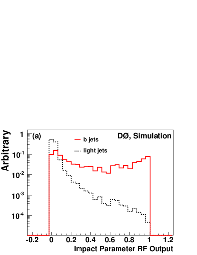
VII.1 Input variables
VII.1.1 Impact Parameter Variables
To train the RF based on variables derived from the impact parameter properties we combine the following variables:
1.
the output of the JLIP algorithm;
2.
the output of the CSIP algorithm;
3.
the reduced JLIP bid_nim , which is computed by removing the track with the
lowest probability of originating from the PV and then recalculating the JLIP;
4.
the combined probability bid_nim associated with the tracks with the highest
and second highest probability of coming from the PV;
5.
the largest separation in
between any two tracks within a jet, ;
6.
the sum of the distances between each track matched to the jet and the center of the calorimeter jet,
;
7.
the -weighted width of the tracks relative to the calorimeter jet defined as
(1)
8.
the total transverse momentum of all tracks in the jet cone;
9.
the total number of tracks matched to the jet.
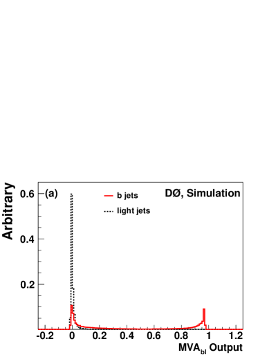
The resulting RF output distribution is displayed in Fig. 1(a).
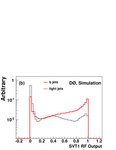
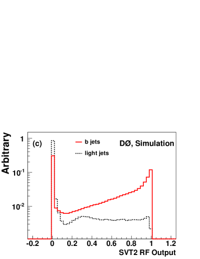
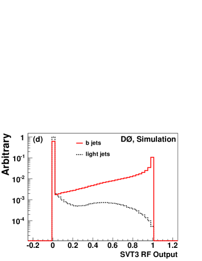
VII.1.2 Secondary Vertex Variables
The SVT algorithms preselect a set of tracks according
to their kinematic properties and reconstruction quality.
As a consequence, starting from a common set of tracks, the various SVT configurations
lead to different secondary vertices with different properties providing a complementary
set of variables for each jet.
We then train five RFs using variables associated with the secondary vertices.
In total each of the SVT RFs uses 29 input variables:
1.
the of the highest track matched to the secondary vertex, ;
2.
the of the second highest track matched to the secondary vertex, ;
3.
the fraction carried by the tracks from the secondary vertex tracks, ;
4.
the number of tracks originating from the secondary vertex;
5.
the mass of the secondary vertex (M), calculated by summing
all track four-momentum vectors assuming that all tracks originate from pions;
6.
the signed decay length significance of the secondary vertex in the plane transverse to the beam direction;
7.
the JLIP probability of the tracks matched to the secondary vertex;
8.
the sum of of the tracks matched to the secondary vertex;
9.
the number of secondary vertices which can be reconstructed from the tracks matched to the jet;
10.
the signed IP of the track with the highest momentum measured transverse to the direction of the secondary vertex;
11.
the number of tracks matched to the jets;
12.
The proper lifetime of the secondary vertex, computed using M, in the plane transverse to the beam direction;
13.
the decay length of the secondary vertex in the plane transverse to the beam direction;
14.
the decay length of the secondary vertex in the beam direction;
15.
the of the highest track in the jet divided by the of the secondary vertex (), ;
16.
the of the second highest track normalized
to the secondary vertex , ;
17.
the of the secondary vertex to the PV in the plane transverse to the beam;
18.
the of the secondary vertex to the PV in the beam direction;
19.
the of the track which has the highest momentum measured relative
to the direction of the secondary vertex;
20.
the momentum of the secondary vertex in the plane transverse to the calorimeter jet direction;
21.
the of the highest track divided by the total jet , ;
22.
the of the second highest track divided by to total jet , ;
23.
the angle between the tracks emerging from the secondary vertex projected into the plane transverse to the beam direction;
24.
the angle between the tracks emerging from the secondary vertex projected in the beam direction;
25.
the (as defined above) as measured for tracks matched to the secondary vertex;
26.
the of the tracks matched to the secondary vertex;
27.
the weighted charge () of the jet, measured as ;
28.
the signed decay length significance of the secondary vertex in the beam direction;
29.
the radius of the cone enclosing all the tracks matched to the secondary vertex.
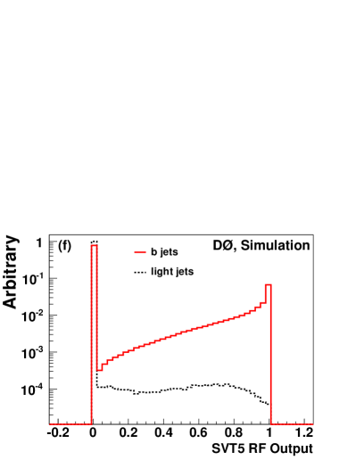
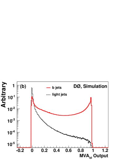
The outputs of the five SVT RFs are shown in Figs. 1(bf).
Figure 1: (color online) Distributions of the six RF outputs for (a) the impact parameter variables
and (bf) the five configurations of the SVT algorithm.
VII.2 Optimized parameters
The outputs of the six RFs, shown in Fig. 1, are combined
using an MLP neural network into a single variable. The training parameters
for the six separate RFs and the final MLP are optimized to minimize
the misidentification rate for a fixed jet identification efficiency.
The RF parameters are the number of trees in the forest (5) and
the number of variables considered at each random split (all).
The parameters used for building the final neural network discriminant
are the number of nodes (7 input, 1 hidden, and 1 output) and the
number of training iterations (50).
VII.3 performance in simulation
The performance of the algorithm is presented in Fig. 2.
A measure of the discriminating power is given by the performance profile, or the identification
efficiency of a jet versus the misidentification rate.
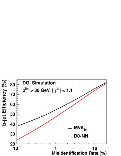
The comparison of the performance of the D0-NN and algorithms is presented in Fig. 3.
At low values of the misidentification rate, the preforms significantly better than the D0-NN,
while at high values they are similar.
We define a set of benchmark points, designated as operating points (OPs) below, and determine the efficiency and
misidentification rates of the OPs for use in subsequent analyses. For the algorithm, these points are
defined in the following way:
L6, ;
L5, ;
L4, ;
L3, ;
L2, ;
Loose, ;
oldLoose, ;
Medium, ;
Tight, ;
VeryTight, ;
UltraTight, ;
MegaTight, .
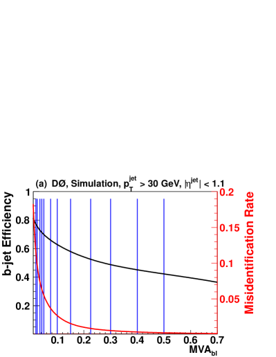
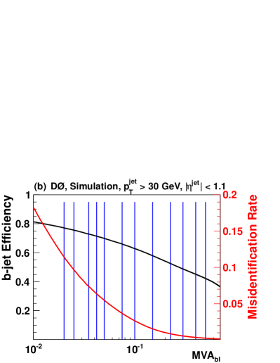
These OPs are displayed in Fig. 4 where the
identification efficiency for jets and the misidentification
rate for light jets are shown as a function of the output
for simulated events.
Figure 2: (color online) The output for light flavored and jets in MC events, with (a) linear and (b) logarithmic scales. Both distributions are normalized to unity.Figure 3: (color online) The performance of the and D0-NN algorithms for jets with
and GeV.
Figure 4: (color online) The efficiency for selecting a jet and the light jet misidentification rate
as a function of the requirement as determined in simulations. The vertical lines
correspond to the selected operating points described in Sec. VII.3, with (a) linear and (b) logarithmic scales.
VIII Efficiency Estimation
Once the algorithm has been defined and its performance is quantified in simulation,
we compare the performance measured in data.
This is a two step-process where we use the efficiencies
in both data and MC to correct the simulation.
VIII.1 System8 method
Using the System8 (S8) formalism, the jet identification efficiencies
can be measured directly from data bid_nim .
A system of eight equations with eight unknowns is
constructed so that solution to these nonlinear equations
includes the efficiency for selecting jets.
To determine the efficiency of identifying a jet we construct
a heavy flavor enriched data sample. These events contain two
back-to-back jets satisfying , one jet must
have GeV and and
be matched to a muon inside a cone of around its centroid (called a muonic jet).
The matched muon must have GeV.
These events, now enriched in heavy flavor
jets, contain contamination from light jets due to muonic decays of and .
Since the S8 method only accommodates a single background we combine the
and light jet backgrounds into a single sample referred to as “ jets”.
Three additional requirements, or “tags”, are individually applied
to muonic jets to create subsamples that are further enriched in jets.
The first tag selects muonic jet that passes a given OP
(described in Sec. VII.3).
The second tag is a requirement on
relative to the direction obtained by adding the muon and jet momenta, known as .
Requiring that GeV removes light jets as the large
quark mass leads to large muon Hedin .
The final tag is a requirement that the jet which is recoiling from the muonic jet has , this is known as the “away-side tag”.
The “away-side tag” allows us to select a data sample heavily enriched in pair-produced back-to-back jets.
Using the JLIP to tag this away jet leads to an enrichment in the overall heavy flavor content
without applying any additional requirements on the muonic jet.
The following coefficients are introduced into the S8 formulation to
account for possible correlations between these tags:
: Correlations between the away tag and requirements for jets.
: Correlations between the away tag and requirements for jets.
: Correlations between the and requirements for jets.
: Correlations between the and requirements for jets.
The above tags are denoted as , for the requirement; , for the requirement; and, , for the away tag. These are applied both individually and concurrently and will appear as superscripts in the following system of S8 equations:
(10)
where the subscripts and refer either to or jets,
refers to the fraction of the total number of selected jets in the sample
that pass a given tag, denotes the fraction of events of
a given flavor in the initial un-tagged sample, and
refers to the efficiency of a jet of flavor passing tag . is determined
from the data and , , , and are determined
from simulations bid_nim .
This leaves eight remaining unknowns which form the solution, including the
variable we are interested in: , the efficiency of a jet passing the requirement.
These equations give two possible solutions for
but this can be resolved by requiring that
.
The jet identification efficiency obtained with the S8 method is valid for
muonic jets. To obtain the efficiency for inclusive jet decays,
a correction factor is determined by using two samples of
simulated jets: muonic and inclusive.
The final efficiency is then defined as
(11)
where
is the data-to-simulation efficiency correction factor,
is the efficiency for passing all OPs as measured by the S8,
and is the efficiency measured in simulation.
The identification efficiency for jets is not measured directly from the data.
It is assumed that the data-to-simulation scale factor is
identical for and jets bid_nim . The jet identification efficiency
is then derived from the simulation as
(12)
VIII.2 efficiency
Using this methodology we are able to determine for the set of OP requirements.
We have selected two OPs, Loose and Tight, for demonstration.
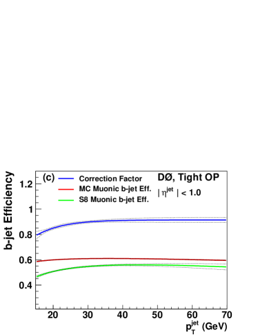
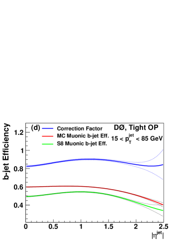
In Fig. 5 the efficiency for identifying a muonic jet, , is shown
for data and MC. The ratio of these
two efficiencies, , is also displayed.
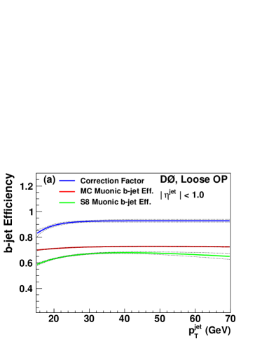
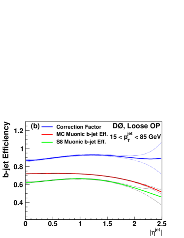
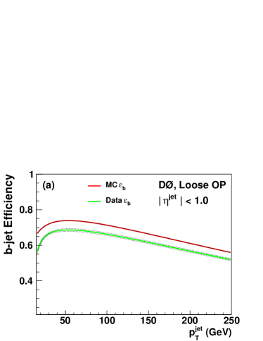
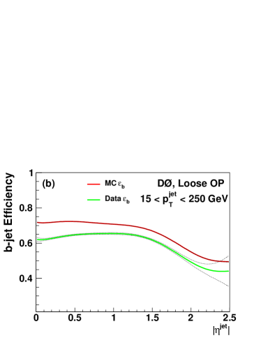
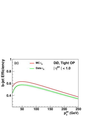
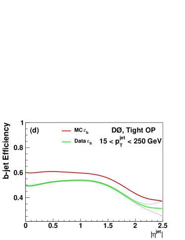
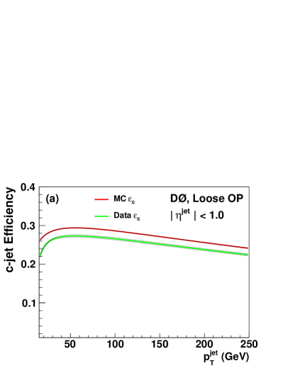
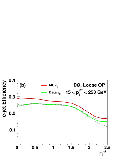
Figs. 6 and 7 show the MC and data corrected
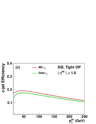
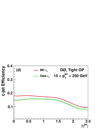
efficiencies for and jets in dijet events, respectively.
The data efficiency curves are corrected with the parameterized correction
factor derived in Fig. 5.
Finally, in Fig. 8, we present the total systematic uncertainty
for the S8 method on , discussed in Ref. bid_nim , parameterized as a function of jet .
Figure 5: (color online) The efficiency for selecting a muonic -jet in MC and data using the S8 method. The correction factor, , which is used to model the algorithm’s efficiency, is also shown. Two OPs are shown (a,b) the Loose and (c,d) Tight. The efficiencies are parameterized as a function of (a,c) , for central jets and versus (b,d) . The band which surrounds the lines corresponds to total uncertainties.
Figure 6: (color online) The MC jet identification efficiency, as measured in dijet events along with the data jet identification efficiency. Two OPs are shown (a,b) the Loose and (c,d) Tight. The efficiencies are parameterized as a function of (a,c) , for central jets and versus (b,d) .
Figure 7: (color online) The MC jet identification efficiency, as measured in dijet events along with the data jet identification efficiency. Two OPs are shown (a,b) the Loose and (c,d) Tight. The efficiencies are parameterized as a function of (a,c) , for central jets and versus (b,d) .
Figure 8: (color online) The total uncertainty on from the S8 method as a function of for two choices of OPs (a) Loose and (b) Tight.
IX Misidentification Rate Determination
A precise understanding of the misidentification rates is especially important
in searches for rare processes which can be overwhelmed by large backgrounds.
Previous methods bid_nim ; cdfhobit ; cmsbtag to determine this
rate relied heavily on simulation.
The method in Ref. bid_nim for estimating the misidentification
rate uses “negatively tagged” (NT) jets, or those with negative IP, with input from simulation.
Here we present the SystemN (SN) method which
extracts misidentification rates directly from data.
IX.1 SystemN method
The SN method uses a series of linear equations to describe the efficiency for light jets to satisfy the various OPs.
Using a data sample of inclusive dijet events (the inclusive jet sample) we separate events as determined by the OP boundaries.
If we have OPs, then there will be +1 bins, with each bin
containing all the jets between the two consecutive OP’s values.
An equation relating the number of jets of each flavor, along with
their identification efficiencies, to the total number of retained jets in
each bin is formed:
(13)
where is the number of selected jets in that bin,
is the efficiency to identify a jet of flavor , and
is the number of jets of flavor in the total sample.
The measured and jet efficiencies from the S8 method are
used to predict the rate for selecting and jets in each bin.
For example, the equations describing a selection of five arbitrary
OPs is given below (a total of twelve OPs are defined in the real analysis):
(20)
where is the efficiency for selecting a jet of flavor
between the the and OP boundaries. The anti-OP1 point, aOP1,
is the set of all jets which fall below the OP1 requirement.
The number of jets of a given flavor, , can be extracted from the data using
a template fit based on the M distributions corresponding to each jet flavor, as described below.
IX.2 Sample composition
A measurement of the overall flavor composition is obtained by fitting M templates
for , , and light jets to a data distribution.
These fits provide the number of and jets after the and SVT requirements,
and .
Applying these requirements creates a sample enriched in heavy flavor jets.
The sample composition of the inclusive jet sample
is calculated by extrapolating from this heavy flavor sample using and jet selection
efficiencies measured using the S8 procedure for jets passing and SVT
requirements. The data sample is divided into several jet and bins to provide
a parameterization of the sample composition.
Data is used to estimate the M template shapes for the
different jet flavors.
For the and jet M templates, a data-to-MC correction factor is
estimated by comparing the M distributions in a separate data sample (described in Sec. IX.2.1)
to the MC templates on a bin-by-bin basis.
For light jets, M template shapes are estimated using a data sample
enriched in light jets, described in Sec. IX.2.2.
IX.2.1 Corrections to the heavy flavor templates
To obtain an estimate of the shape of the heavy flavor jet M distribution from data, a heavy flavor
enriched dijet sample is constructed by requiring:
•
Two taggable jets with a separation of .
•
A jet must be selected by passing both an and SVT requirement.
•
The recoiling jet must be matched to a muon, GeV, and pass a SVT requirement with M GeV.
The ratio of the data M distribution and the MC predicted M templates
for , , and light jets are used to create a correction factor. To determine the
normalization of the MC templates the predicted sample composition is taken from the MC.
This correction factor is then applied to the MC and jet M templates to correct their shape
to the data in separate jet and bins,
an example of the corrected mass template is shown in Fig. 9.
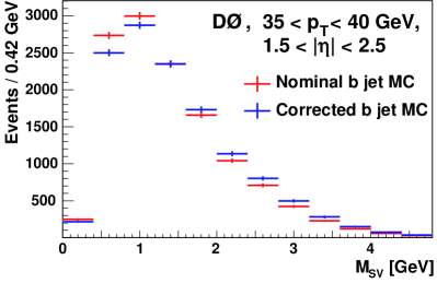
Figure 9: (color online) Comparison of MC and data corrected jet M template shapes for jets with and . The data corrected M template uses a shape reweighting derived in Sec. IX.2.1.
IX.2.2 Data driven light jet templates
The light jet templates are estimated from M distribution of jets in a NT data sample bid_nim .
This sample comprises jets having a negative IP and passing an SVT selection.
The shape of the M distribution corresponding to this sample is affected by
contamination due to the presence of heavy flavor jets and as such
is not a perfect representation of the light jet M shape in data. The NT template shapes
are measured from data in each and interval.
Fig. 10 shows a comparison between the NT M distribution and the MC light jet template.
The difference in the shapes is taken as a systematic uncertainty.
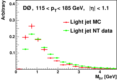
Figure 10: (color online) Comparison of the MC light jet and NT M mass templates for jets with and GeV. The difference is taken as a measure of the systematic uncertainty due to residual contamination from
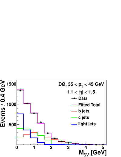
heavy flavor jets in the NT data.Figure 11: (color online) An example of the sample composition fit using the M for jets which
pass and SVT requirements and have and .
The , , and light jets are fit to the data resulting in the total fitted distribution.
IX.2.3 Sample composition measurement
The data driven templates obtained above are used to fit the M distribution in data using a log-likelihood fitter
in bins of jet and . An example of a fit to the M distribution
using the , , and light jet templates is shown in Fig. 11.
This results in a measurement of the fraction of each flavored jet type in that bin.
The fits in each of the and regions
are subsequently extrapolated back to the full inclusive jet sample using
the and jet efficiency distributions measured for the and SVT
algorithms. The number of events of heavy flavor, (either or ),
in the inclusive jet sample is calculated using the following formula:
(21)
where is the fraction of jets with flavor extracted from the heavy flavor
enriched sample and is the S8 efficiency for a and SVT requirements, and is the total
number of events in that bin.
The efficiency is calculated for the average and of the jets in the region.
While can be corrected to the inclusive jet sample, the light jet
fraction cannot be. The corresponding light jet fraction in the inclusive jet sample
is then determined from .
The parameterization of the inclusive jet sample composition is important to obtain
the misidentification rate as a function of and
to minimize the effect of statistically limited bins at high . However, the choice of
parameterization is not straightforward.
The optimal parameterizations were determined by considering the probability of various functional forms,
typically a first order polynomial or a second order logarithmic polynomial.
IX.3 Solutions of the SystemN equations
Instead of solving Eq. 20 analytically, we form a likelihood to improve the
stability of the solutions. In this likelihood
we take the equations and compare them to what is predicted from simulations.
We allow the extracted flavor fractions, , to float within their uncertainties during
this fit. To help constrain this likelihood a second set of SN equations is built
using a new data sample, the full procedure
is repeated and added to the likelihood fit. This new sample is a sub-set
of the inclusive jet sample which has the additional requirement that the recoiling “away jet” must be matched to a muon. This
sample is defined as the “away jet sample”.
The resulting likelihood is formed by summing over each of the OP bins for both samples:
(22)
where is the number of data events in sample , either inclusive or away jet sample,
in the interval , is the
predicted number of events in OP bin .
A normalization factor, , is used to ensure that the likelihood values remain well defined:
(23)
which is then subtracted from the likelihood.
We use the and jet fractions measured in the previous section to help
stabilize the fit through a term which is added to the likelihood:
(24)
is a covariance error matrix resulting from
the extraction of the and jet content from the M fit and is a vector
(25)
where is the number of jets, of flavor , estimated from the M template fits,
and are the number of jets, of flavor , in the inclusive sample.
The result of this likelihood fit is the extraction of the final data driven light jet efficiency parameterized over jet
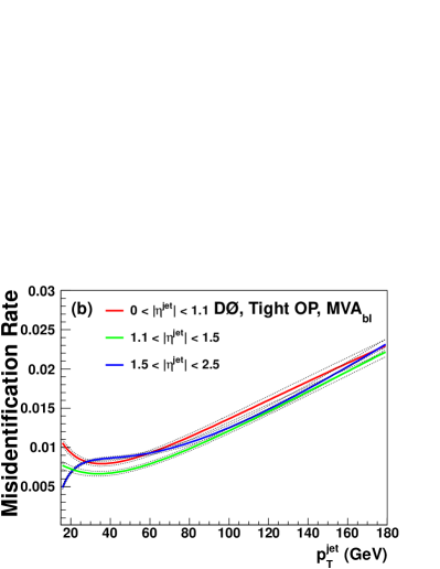
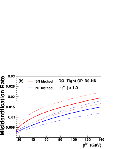
and in OP bins. These misidentification rates are shown in Fig. 12.
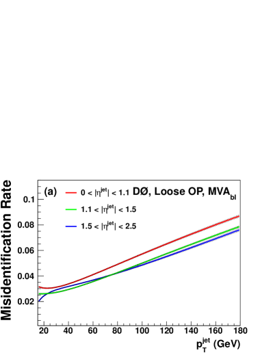
Figure 12: (color online) The SN data driven misidentification rates for the algorithm.
Two OPs are shown (a) Loose and (b) Tight.
These are further parameterized over jet and for three different jet intervals:
, , and .
The black dotted lines represent the uncertainty on the fit.
IX.4 SystemN systematic uncertainties
The three dominant systematic uncertainties on the misidentification rates are:
•
The shape of the and jet M templates
•
The shape of the light jet M template
•
The uncertainty on the and jet efficiencies from the S8 method
Heavy flavor template shape.
The effect of imperfections in the modeling of the and jet M templates is
estimated by carrying out the sample composition measurement using a set of
heavy flavor M templates which are not corrected to data in each of the and
intervals. The full difference between the MC and data corrected sample composition
predictions is used as an uncertainty. As described in Sec. IX.2.1, the heavy flavor templates
are derived using MC inputs. These inputs are then varied and the largest deviation from the nominal shape
is used to provide an additional uncertainty.
Light flavor template shape.
The uncertainty due to the shape of the light jet M templates is estimated by
performing the sample composition fit using both the NT and MC light jet
template shapes, taking the difference in the sample composition to assign
an uncertainty.
and jet efficiency uncertainty.
When extrapolating the flavor fractions, measured in the heavy flavor enriched sample,
to the inclusive jet sample the efficiencies from the S8 method are used. To account for the
uncertainties inherited in this procedure it is repeated after the efficiencies are varied by
. This variation will only affect the extrapolation procedure.
The parameterization of the systematic uncertainties is evaluated by carrying out closure tests, where
the percentage difference between the number of actually
selected jets and the predicted number of jets in various
bins in and regions are compared. The uncertainty
is determined from the RMS of the resulting distributions.
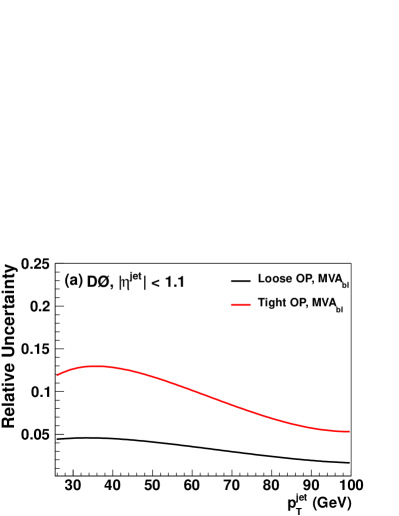
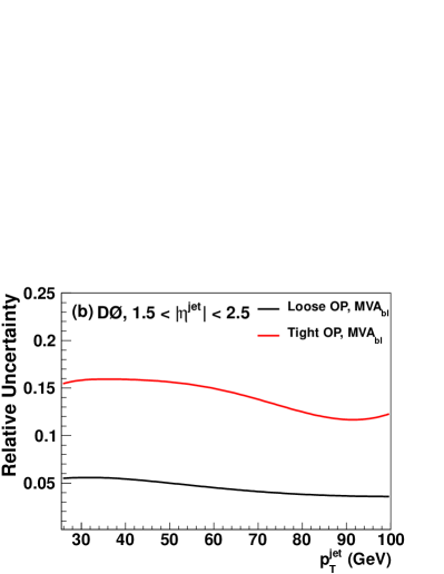
The total uncertainty on the data-driven misidentification rate attained
using the SN method, given by the statistical and systematic uncertainties
combined in quadrature, is shown in Fig. 13 for the Loose and Tight
OPs of the algorithm.
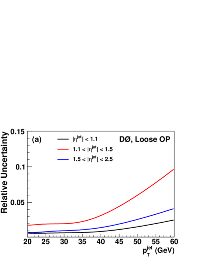
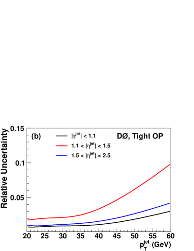
Figure 13: (color online) The total relative uncertainty on the misidentification rate from the SN method
parameterized in terms of jet and for two different regions:
(a) and (b) .
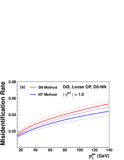
IX.5 Comparison with previous method
A comparison between the misidentification rates of the D0-NN algorithm measured using the SN
method and those estimated by the NT method of Ref. bid_nim is shown in
Fig. 14. Both provide comparable uncertainties.
For the looser OPs the central value of the new method gives
a misidentification rate roughly higher than the central values for the previous method,
and for the tighter OPs the difference is closer to .
The two methods do agree with each other within uncertainties across the full range
of jet , but the misidentification rate for the NT method is systematically lower.
Figure 14: (color online) Comparison between the misidentification rates of the
D0-NN derived for two OPs, (a) Loose and (b) Tight, using the new SN method
and the old method described in Ref. bid_nim .
The dashed bands which surround the values correspond to the total uncertainties.
The source of this difference comes from the use of simulation in the NT method.
With the removal of the s the main source of misidentified light jets comes from
detector resolution and track mis-reconstruction effects.
The simulation does not accurately reproduce these effects by modeling ideal detector responses
and the resulting misidentification rate as determined by the NT method is systematically underestimated.
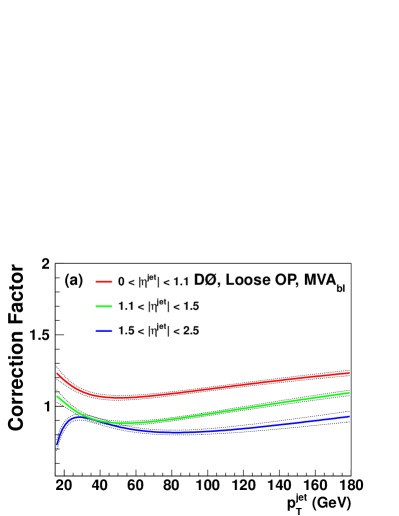
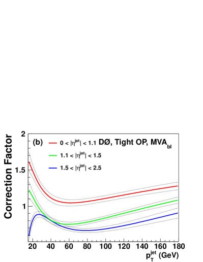
IX.6 misidentification rates
Figure 15: (color online) The misidentification rate correction factors for the light jet MC which are derived by taking the ratio
of the data and MC misidentification rates. Two OPs are shown, (a) Loose and (b) Tight.
These are further parameterized over jet and for three different jet intervals:
, , and .
The black dotted lines represent the uncertainty on the fit.
The final results are the misidentification rate for light jets extracted from our data, as shown in Fig. 12.
These are parameterized in terms of for three different regions.
This data-driven measurement of the misidentification rate can be combined with that
modeled in simulation and we can derive a MC correction factor, as shown in Fig. 15.
These correction factors are applied in the light jet simulations (for jets passing the requirements).
Table 2 shows the responses, efficiencies, and misidentification rates, of the algorithm as measured in data.
Table 2: The efficiency of selecting a , , or light jet using the as determined
by using the S8 and SN method directly from data for 12 OPs.
The total uncertainties are included along with the OP definitions.
OP Name
Min.
L6
0.02
L5
0.025
L4
0.035
L3
0.042
L2
0.05
Loose
0.075
oldLoose
0.1
Medium
0.15
Tight
0.225
VeryTight
0.3
UltraTight
0.4
MegaTight
0.5
X Summary and Conclusions
The identification of heavy flavor jets is a crucial component of particle physics analyses.
Utilizing the unique characteristics of the fragmenting quark we created algorithms
which allow for the identification of jets with high efficiency and purity.
The algorithm shows improvements over previous algorithms utilized at D0.
For a light jet misidentification rate of 1% we observe an
improvement in the efficiency over the D0-NN algorithm for selecting a jet of 15% per jet.
A new method for extracting the misidentification rate directly from data has also been presented.
The data-derived misidentification rates of the SystemN method are compatible within uncertainties
with previous simulation-based methods, however a systematic difference is observed. This difference is due
to the limited ability of the simulation to accurately model resolution and track mis-reconstruction effects.
By removing this dependence on simulation the SystemN method provides a
more accurate and reliable measurement of the light jet misidentification rates in data.
Acknowledgement
We thank the staffs at Fermilab and collaborating institutions,
and acknowledge support from the
DOE and NSF (USA);
CEA and CNRS/IN2P3 (France);
MON, NRC KI and RFBR (Russia);
CNPq, FAPERJ, FAPESP and FUNDUNESP (Brazil);
DAE and DST (India);
Colciencias (Colombia);
CONACyT (Mexico);
NRF (Korea);
FOM (The Netherlands);
STFC and the Royal Society (United Kingdom);
MSMT and GACR (Czech Republic);
BMBF and DFG (Germany);
SFI (Ireland);
The Swedish Research Council (Sweden);
and
CAS and CNSF (China).
References
(1)
V. Abazov et al., [D0 Collaboration],
Nucl. Instrum. Methods Phys. Res. A 620, 490 (2010).
(2)
J. Freeman et al.,
Nucl. Instrum. Methods Phys. Res. A 697, 64 (2013).
(3)
S. Chatrchyan et al., [CMS Collaboration],
JINST 8, P04013 (2013).
(4)
V. Abazov et al., [D0 Collaboration],
Nucl. Instrum. Methods Phys. Res. A 565, 463 (2006).
(5)
S. Ahmed et al., [D0 Collaboration],
Nucl. Instrum. Methods Phys. Res. A 634, 8 (2011).
(6)
S. Abachi et al., [D0 Collaboration],
Nucl. Instrum. Methods Phys. Res. A 324, 53 (1993).
(7)
B. Casey et al.,
Nucl. Instrum. Methods A698, 208 (2013).
(8)
T. Sjostrand et al.,
Comput. Phys. Commun. 135, 238 (2001).
(9)
D. Lange,
Nucl. Instrum. Methods Phys. Res. A 462, 152 (2001).
(10)
R. E. Kalman,
Transactions of the ASME–Journal of Basic Engineering 82, 35
(1960).
(11)
G. C. Blazey et al.,
arXiv:hep-ex/0005012, (2000).
(12)
V. M. Abazov et al., [D0 Collaboration],
arXiv:hep-ex/13126873, (2013).
(13)
A. Hocker et al.,
PoS ACAT, 040 (2007).
(14)
R. Brun and F. Rademakers,
Nucl. Instrum. Methods Phys. Res. A 389, 81 (1997).
(15)
D. Hedin, T. Kramer, and K. Roberts,
C87-11-11 (1987).