Probabilistic Archetypal Analysis

Abstract

Archetypal analysis represents a set of observations as convex combinations of pure patterns, or archetypes. The original geometric formulation of finding archetypes by approximating the convex hull of the observations assumes them to be real valued. This, unfortunately, is not compatible with many practical situations. In this paper we revisit archetypal analysis from the basic principles, and propose a probabilistic framework that accommodates other observation types such as integers, binary, and probability vectors. We corroborate the proposed methodology with convincing real-world applications on finding archetypal winter tourists based on binary survey data, archetypal disaster-affected countries based on disaster count data, and document archetypes based on term-frequency data. We also present an appropriate visualization tool to summarize archetypal analysis solution better.

1 Introduction

Archetypal analysis (AA) represents observations as composition of pure patterns, i.e., archetypes, or equivalently convex combinations of extreme values (Cutler and Breiman, 1994). Although AA bears resemblance with many well established prototypical analysis tools, such as principal component analysis (PCA, Mohamed et al, 2009), non-negative matrix factorization (NMF, Févotte and Idier, 2011), probabilistic latent semantic analysis (Hofmann, 2013), and $k$-means (Steinley, 2006); AA is arguably unique, both conceptually and computationally. Conceptually, AA imitates the human tendency of representing a group of objects by its extreme elements (Davis and Love, 2010): this makes AA an interesting exploratory tool for applied scientists (e.g., Eugster, 2012; Seiler and Wohlrabe, 2013). Computationally, AA is data-driven, and requires the factors to be probability vectors: these make AA a computationally demanding tool, yet brings better interpretability.

The concept of AA was originally formulated by Cutler and Breiman (1994). The authors posed AA as the problem of learning the convex hull of a point-cloud, and solved it using alternating non-negative least squares method. In recent years, different variations and algorithms based on the original geometrical formulation have been presented (Bauckhage and Thurau, 2009; Eugster and Leisch, 2011; Mørup and Hansen, 2012). However, unfortunately, this framework does not tackle many interesting situations. For example, consider the problem of finding archetypal response to a binary questionnaire. This is a potentially useful problem in areas of psychology and marketing research that cannot be addressed in the standard AA formulation, which relies on the observations to exist in a vector space for forming a convex hull. Even when the observations exist in a vector space, standard AA might not be an appropriate tool for analyzing it. For example, in the context of learning archetypal text documents with tf-idf as features, standard AA will be inclined to finding archetypes based on the volume rather than the content of the document.

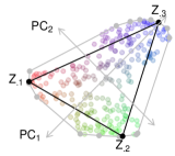
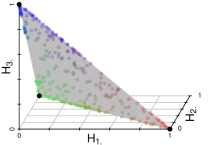
Figure 1: (a) Illustration of archetypal analysis with three archetypes Z, and (b) the corresponding factors H, projections of the original observations on the convex hull of the archetypes; (a) also explicates the difference between PCA and AA.

In this paper we revisit archetypal analysis from the basic principles, and reformulate it to extend its applicability. We admit that the approximation of the convex hull, as in the standard AA, is indeed an elegant solution for capturing the essence of ‘archetypes’, (see Figure 1a and 1b for a basic illustration). Therefore, our objective is to extend the current framework, not to discard it. We propose a probabilistic foundation of AA, where the underlying idea is to form the convex hull in the parameter space. The parameter space is often vectorial even if the sample space is not (see Figure 2 for the plate diagram). We solve the resulting optimization problem using majorization-minimization, and also suggest a visualization tool to help understand the solution of AA better.

The paper is organized as follows. In Section 2, we start with an in-depth discussion on what archetypes mean, and how this concept has evolved over the last decade, and has been utilized in different contexts. In Section 3, we provide a probabilistic perspective of this concept, and suggest probabilistic archetypal analysis. Here we explicitly tackle the cases of Bernoulli, Poisson and multinomial probability distributions, and derive the necessary update rules (derivations available as appendix). In Section 4, we discuss the connection between AA and other prototypical analysis tools—a connection that has also been partly noted by other researchers (Mørup and Hansen, 2012). In Section 5 we provide simulations to show the difference betweeen probabilistic and standard archetypal analysis solutions. In Section 6, we discuss a visualization method for archetypal analysis, and present several improvements. In Section 7, we present an application for each of the above observation models: finding archetypal winter tourists based on binary survey data; finding archetypal disaster-affected countries based on disaster count data; and finding document archetypes based on term-frequency data. In Section 8 we summarize our contribution, and suggest future directions.

Distribution	Notation	Parameters	pdf/pmf
Normal	$\mathcal{N}(\boldsymbol{\mu},\boldsymbol{\Sigma})$	$\boldsymbol{\mu}\in\mathbb{R}^{K}$, $\boldsymbol{\Sigma}\in\mathbb{R}^{K\times K}$	$(2\pi)^{-\frac{K}{2}}|\boldsymbol{\Sigma}|^{-\frac{1}{2}}\exp\{-\frac{1}{2}(\boldsymbol{x}-\boldsymbol{\mu})^{\prime}\boldsymbol{\Sigma}^{-1}(\boldsymbol{x}-\boldsymbol{\mu})\}$
Dirichlet	$\mathrm{Dir}(\boldsymbol{\alpha})$	$\boldsymbol{\alpha}=(\alpha_{1},\ldots,\alpha_{K})$, $K>1$, $\alpha_{i}>0$	$\frac{1}{\mathrm{B}(\alpha)}\prod^{K}_{i=1}x^{\alpha_{i}-1}_{i}$ where $\mathrm{B}(\alpha)=\frac{\prod^{K}_{i=1}\Gamma(\alpha_{i})}{\Gamma(\sum^{K}_{i=1}\alpha_{i})}$
Poisson	$\mathrm{Pois}(\lambda)$	$\lambda>0$	$\frac{\lambda^{x}}{x!}\exp\{-x\}$
Bernoulli	$\mathrm{Ber}(p)$	$0<p<1$	$p^{x}(1-p)^{1-x}$
Multinomial	$\mathrm{Mult}(n,\bf{p})$	$n>0$, $\boldsymbol{p}=(p_{1},\ldots,p_{K})$, $\sum^{K}_{i=1}p_{i}=1$	$\frac{n!}{x_{1}!\cdots x_{K}!}p_{1}^{x_{1}}\cdots p_{K}^{x_{K}}$

Table 1: Distributions used in the paper.

Throughout the paper, we represent matrices by boldface uppercase letters, vectors by boldface lowercase letter, and variables by normal lowercase letter. 1 denotes the row vector of ones, and I denotes the identity matrix. Table 1 provides the definitions of the distributions used throughout the paper. Implementations of the presented methods are available at http://aalab.github.io/.

2 Review

The goal of archetypal analysis is to find archetypes, ‘pure’ patterns. In Section 2.1 we provide some intuition on what these pure patterns imply. In Section 2.2, we discuss the mathematical formulation of this archetypal analysis as suggested by Cutler and Breiman (1994). In Section 2.3 we discuss how this concept has been utilized since its inception: here, we point out key references, important developments, and convincing applications.

2.1 Intuition

Archetypes are ‘ideal example of a type’. The word ‘ideal’ does not necessarily have a qualitative meaning of being ‘good’, but this concept is mostly subjective. For example, one can consider ideal example to be a prototype, and other objects to be variations of such prototype. This view is close to the concept of clustering, where the centers of the clusters are the prototypes. For archetypal analysis, however, ideal example has a different meaning. Intuitively it implies that the prototype can not be surpassed, its the purest or the most extreme that can be witnessed. A simple example of archetypes are the colors red, blue and green (cf. Figure 1a) in the RGB color space: any other color can be expressed as combinations of these ideal colors. Another example can be comic book superheros who excel in some unique characteristics, say speed or stamina or intelligence, more than anybody with these abilities: they are the archetypal superheros with that particular ability. The non-archetypal superheroes, on the other hand, possess “many” abilities that are not extreme. It is to be noted that a person with all the abilities to their full realizations, if exists, is an archetype, Similarly, if one considers normal humans alongside super-humans then a person with none of these abilities is also an archetype.

In both these examples, the archetypes are rather trivial. If one represents each color in the RGB space then it is obvious that the unit vectors R, G and B are pure colors or archetypes. Similarly, if one represents every (super-)human in a two dimensional normalized scale of strength and intelligence, then there are four extreme instances, and hence archetypes are: first and second, person with highest score in either of these attributes and none in the other; third and fourth, person with highest/lowest score in both these attributes. However, in reality one may not observe these attributes directly, but some other features. For example, one can describe a person with many personality traits, such as humor, discipline, optimism, etc., but these characteristics cannot be measured directly. However, one can prepare a questionnaire (or observed variables) that explores these (latent) personality traits. From this questionnaire, curious users can attempt to identify archetypal humans, say an archetypal leader or an archetypal jester.

Finding archetypal patterns in the observed space is a non-trivial problem. It is difficult, in particular, since the archetype itself may not be belong to the set of observed samples but should be inferred; yet, it should also not be a “mythological”, but rather something that might be observed. Cutler and Breiman (1994) suggested a simple yet elegant useful solution that finds the approximate convex hull of the observations, and define the vertices as archetypes. This allows individual observations to be best represented by composition (convex combination) of archetypes, while archetypes can only be expressed by themselves, i.e., they are the ‘purest form’ or ‘most extreme’ forms. Although, it is certainly not the most desired solution, since, the inferred archetypes are restricted to be on the boundary of the convex hull of the observations, whereas true archetype may be outside; inferring such archetypes outside the observation hull will require strong regularity assumptions. The solution suggested by Cutler and Breiman (1994) finds a trade off between computational simplicity, and the intuitive nature of archetype.

2.2 Formulation

Cutler and Breiman posed AA as the problem of learning the convex hull of a point-cloud. They assumed the archetypes to be convex combinations of observations, and the observations to be convex combinations of the archetypes. Let X be a (real-valued) data matrix with each column as an observation. Then, this is equivalent to solving the following optimization problem:

$$\min_{\textbf{W},\textbf{H}}||\textbf{X}-\textbf{X}\textbf{W}\textbf{H}||^{2}_{\mathrm{F}}$$ (1)

with the constraint that both W and H are column stochastic matrices. $\mathrm{F}$ denotes Frobenious norm. Given $N$ observations, and $K$ archetypes, W is $N\times K$ dimensional, and H is $K\times N$ dimensional matrices. Here, $\textbf{Z}=\textbf{X}\textbf{W}$ are the inferred archetypes that exist on the convex hull of the observations due to the stochasticity of W and for each $n$-th sample $\textbf{x}_{n}$, $\textbf{Z}\textbf{h}_{n}$ is its projection on the convex hull of the archetypes.

Cutler and Breiman solved this problem using an alternating non-negative least squares method as follows:

$$\textbf{H}^{t+1}=\mbox{arg\,min}_{\textbf{H}\geq\textbf{0}}||\textbf{X}-\textbf{Z}^{t}\textbf{H}||_{\mathrm{F}}^{2}+\lambda||\textbf{1}\textbf{H}-\textbf{1}||^{2}$$

and

$$\textbf{W}^{t+1}=\mbox{arg\,min}_{\textbf{W}\geq\textbf{0}}||\textbf{Z}^{t}-\textbf{X}\textbf{W}||_{\mathrm{F}}^{2}+\lambda||\textbf{1}\textbf{W}-\textbf{1}||^{2}$$

where after each alternating step, the archetypes (Z) are updated by solving $\textbf{X}=\textbf{Z}^{t+1}\textbf{H}^{t}$, and $\textbf{Z}^{t+1}=\textbf{X}\textbf{W}^{t}$, respectively. The algorithm alternates between finding the best composition of observations given a set of archetypes, and then finding the best set of archetypes given a composition of observations. Notice that the stochasticity constraint was cleverly enforced by a suitably strong regularization parameter $\lambda$. The authors also proved that $k>1$ archetypes are located on the boundary of the convex hull of the point-cloud, and $k=1$ archetype is the mean of the point cloud.

2.3 Development

The first publication, to the best of our knowledge, which deals with the idea of “ideal types” and observations related to them, is Woodbury and Clive (1974). There, the authors discuss how to derive estimates of grades of membership of categorical observations, given an a-priori defined set of ideal (or pure) types, in the context of clinical judgment. Twenty years later—in 1994—Cutler and Breiman (1994) formulated archetypal analysis (AA) as the problem of estimating both the membership and the ideal types given a set of real-valued observations. They motivated this new kind of analysis with, among other examples, the estimation of archtyepal head dimensions of Swiss Army soldiers.

One of the original authors continued her work on AA in the fields of physics and applied it on spatio-temporal data (Stone and Cutler, 1996). In this line of research, Cutler and Stone (1997) developed moving archetypes, by extending the original AA framework with an additional optimization step, which estimates the optimal shift of observations in the spatial domain over time. They applied this method to data gathered from a chemical pulse experiment. Other researches took up the idea of AA and applied it in different fields; the following is a comprehensive list of problems where other researchers have applied AA: analysis of galaxy spectra (Chan et al, 2003), ethical issues and market segmentation (Li et al, 2003), thermogram sequences (Marinetti et al, 2007), gene expression data (Thøgersen et al, 2013); performance analysis in marketing (Porzio et al, 2008), sports (Eugster, 2012), and science (Seiler and Wohlrabe, 2013); face recognition (Xiong et al, 2013); and in game AI development (Sifa and Bauckhage, 2013).

In recent years, animated by the rise of the non-negative matrix factorization research, various authors have proposed extensions and variations to the original algorithm. Following are a few notable publications. Thurau et al (2009) introduce the convex-hull non-negative matrix factorization (NMF). Motivated by the convex NMF, the authors make the same assumption as made in AA that observations are convex combinations of specific observations. However, they derive an algorithm which estimates the archetypes not from the entire set of observations but from potential candidates found from 2-dimensional projections on eigenvectors: this leads to a solution also applicable for large data sets. The authors demonstrate their method on a data set consisting of 150 million votes on World of Warcraft${}^{\text{\textregistered}}$ guilds. In Thurau et al (2010), the authors present an even faster approach by deriving a highly efficient volume maximization algorithm. Eugster and Leisch (2011) tackle the problem of robustness, and that a single outlier can break down the archetype solution. They adapt the original algorithm to be a robust M-estimator and present an iteratively reweighted least squares fitting algorithm. They evaluate there algorithm using the Ozone data from the original AA paper with contaminated observations. Mørup and Hansen (2012) also tackle the problem of deriving an algorithm for large scale AA. They propose a solution based on a simple projected gradient method, in combination with an efficient initialization method for finding candidates of archetypes. The authors demonstrate their method, among other examples, with an analysis of the NIPS bag of words corpus and the Movielens movie rating data set.

3 Probabilistic archetypal analysis

We observe that the original AA formulation implicitly exploits a simplex latent variable model, and normal observation model, i.e.,

$$\textbf{h}_{n}\sim\mathrm{Dir}(\textbf{1}),\,\textbf{x}_{n}\sim\mathcal{N}(\textbf{Z}\textbf{h}_{n},\epsilon_{1}\textbf{I}).$$

But, it goes a step further, and generates the loading matrix Z from a simplex latent model itself with known loadings $\boldsymbol{\Theta}\in\mathbb{R}^{M\times N}$, i.e.,

$$\textbf{w}_{k}\sim\mathrm{Dir}(\textbf{1}),\,\textbf{z}_{k}\sim\mathcal{N}(\boldsymbol{\Theta}\textbf{w}_{k},\epsilon_{2}\textbf{I}).$$

Thus, the log-likelihood can be written as,

$$\mathbb{LL}(\textbf{X}|\textbf{W},\textbf{H},\textbf{Z},\boldsymbol{\Theta})=-\frac{\epsilon_{1}}{2}||\textbf{X}-\textbf{Z}\textbf{H}||_{\mathrm{F}}^{2}-\frac{\epsilon_{2}}{2}||\textbf{Z}-\boldsymbol{\Theta}\textbf{W}||_{\mathrm{F}}^{2}+C(\epsilon_{1},\epsilon_{2}).$$

The archetypes Z, and corresponding factors H can then be found by maximizing this log-likelihood (or minimizing the negative log-likelihood) under the constraint that both W and H are stochastic: this can be achieved by alternating optimization as Cutler and Breiman did (but with different update rules for Z, and $\epsilon_{\cdot}$).

The equivalence of this approach to the standard formulation requires that $\boldsymbol{\Theta}=\textbf{X}$. Although unusual in a probabilistic framework, this contributes to the data-driven nature of AA. In the probabilistic framework, $\boldsymbol{\Theta}$ can be viewed as a set of known bases that is defined by the observations, and the purpose of archetypal analysis is to find a sparse set of bases that can explain the observations. These inferred bases are the archetypes, and the stochasticity constraints on W and H ensure that they are the extreme values as one desires. It should be noted that $\boldsymbol{\Theta}_{n}$ does not need to correspond to $\textbf{X}_{n}$: more generally, $\boldsymbol{\Theta}=\textbf{X}\textbf{P}$ where P is a permutation matrix.

Figure 2: Plate diagram of probabilistic archetypal analysis.

3.1 Exponential family

We describe AA in a probabilistic set-up as follows (see Figure 2),

$$\textbf{w}_{k}\sim\mathrm{Dir}(\textbf{1}),\,\textbf{h}_{n}\sim\mathrm{Dir}(\textbf{1}),\,\textbf{x}_{n}\sim\mathrm{EF}(\textbf{x}_{n};\boldsymbol{\Theta}\textbf{W}\textbf{h}_{n})$$

where

$$\mathrm{EF}(\textbf{z};\boldsymbol{\theta})=h(\textbf{z})g(\boldsymbol{\theta})\exp(\eta(\boldsymbol{\theta})^{\top}s(\textbf{z}))$$

with standard meaning for the functions $g,h,\eta$ and $s$. Notice that, we employ the normal parameter $\boldsymbol{\theta}$ rather than the natural parameter $\boldsymbol{\eta}(\boldsymbol{\theta})$, since the former is more interpretable. In fact, the convex combination of $\boldsymbol{\theta}$ is more interpretable than the convex combination of $\boldsymbol{\eta}(\boldsymbol{\theta})$, as a linear combination on $\boldsymbol{\eta}(\boldsymbol{\theta})$ would lead to nonlinear combination of $\boldsymbol{\theta}$. To adhere to the original formulation, we suggest $\boldsymbol{\Theta}_{\cdot n}$ to be the maximum likelihood point estimate from observation $\textbf{X}_{\cdot n}$. Again, the columns of $\boldsymbol{\Theta}$ and X do not necessarily have to be corresponded. Then, we find archetypes $\textbf{Z}=\boldsymbol{\Theta}\textbf{W}$ by solving

$$\mbox{arg\,min}_{\textbf{W},\textbf{H}\geq 0}-\mathbb{LL}(\textbf{X}|\textbf{W},\textbf{H},\boldsymbol{\Theta})\mbox{ such that }\textbf{1}\textbf{W}=\textbf{1},\textbf{1}\textbf{H}=\textbf{1}.$$ (2)

We call this approach probabilistic archetypal analysis (PAA).

The meaning of archetype in PAA is different than in the standard AA since the former lies in the parameter space, whereas the latter in the observation space. To differentiate these two aspects, we call the archetypes $\textbf{Z}=\boldsymbol{\Theta}\textbf{W}$ found by PAA (solving (2)), archetypal profiles: our motivation is that $\boldsymbol{\Theta}_{\cdot n}$ can be seen as the parametric profile that best describes the single observation $\textbf{x}_{n}$, and thus, Z are the archetypal profiles that are inferred from them. We generally refer to the set of indices that contribute to the $k$-th archetypal profile, i.e., $\{i:\textbf{W}_{ik}>\delta\}$, where $\delta$ is a small value, as generating observations of that archetype. Notice that, when the observation model is multivariate normal with identity covariance, then this formulation is the same as solving (1). We explore some other examples of $\mathrm{EF}$: multinomial, product of univariate Poisson distributions, and product of Bernoulli distributions.

3.2 Poisson observations

If the observations are integer valued then they are usually assumed to originate from a Poisson distribution. Then we need to solve the following problem,

$$\mbox{arg\,min}_{\textbf{W},\textbf{H}\geq\textbf{0}}\sum_{mn}\left[-\textbf{X}_{mn}\log(\boldsymbol{\Lambda}\textbf{W}\textbf{H})_{mn}+(\boldsymbol{\Lambda}\textbf{W}\textbf{H})_{mn}\right]$$

such that $\sum_{j}\textbf{H}_{jn}=1\mbox{ and }\sum_{i}\textbf{W}_{ik}=1$. Here $\Lambda_{mn}$ is the maximum likelihood estimate of the Poisson rate parameter from observation $\textbf{X}_{mn}$.

To solve this problem efficiently, we employ a similar technique used by Cutler and Breiman by relaxing the equality constraint with a suitably strong regularization parameter. However, we employ a multiplicative update rule afterwards instead of an exact method like the nonnegative least squares. The resulting update rules are (see Appendix B for derivation)

$$\textbf{H}^{t+1} =\textbf{H}^{t}\odot\frac{\nabla_{\textbf{H}^{t}}^{-}}{\nabla_{\textbf{H}^{t}}^{+}},\,\nabla_{\textbf{H}_{nj}}^{+}=\sum_{im}\boldsymbol{\Lambda}_{im}\textbf{W}_{mn}+\lambda,\nabla_{\textbf{H}_{nj}}^{-}$$

$$=\sum_{i}\frac{\textbf{X}_{ij}\sum_{m}\boldsymbol{\Lambda}_{im}\textbf{W}_{mn}}{\sum_{mn}\boldsymbol{\Lambda}_{im}\textbf{W}_{mn}\textbf{H}_{nj}}+\frac{\lambda}{\sum_{n}\textbf{H}_{nj}}$$

and

$$\textbf{W}^{t+1} =\textbf{W}^{t}\odot\frac{\nabla_{\textbf{W}^{t}}^{-}}{\nabla_{\textbf{W}^{t}}^{+}},\,\nabla_{\textbf{W}_{mn}}^{+}=\sum_{ij}\boldsymbol{\Lambda}_{im}\textbf{H}_{nj}+\lambda,\nabla_{\textbf{W}_{mn}}^{-}$$

$$=\sum_{ij}\frac{\textbf{X}_{ij}\boldsymbol{\Lambda}_{im}\textbf{H}_{nj}}{\sum_{mn}\boldsymbol{\Lambda}_{im}\textbf{W}_{mn}\textbf{H}_{nj}}+\frac{\lambda}{\sum_{m}\textbf{W}_{mn}}\mbox{.}$$

Here $\odot$ denotes Hadamard product. We choose $\lambda$ to be 20 times the variance of the samples.

3.3 Multinomial observations

In many practical problems such as document analysis, the observations can be thought of as originating from a multinomial model. In such cases, PAA expresses the underlying multinomial probability as PWH where P is the maximum likelihood estimate achieved from word frequency matrix X. This decomposition is very similar to PLSA: PLSA estimates a topic by document matrix H and a word by topic matrix Z, while AA estimates a document by topic matrix (W) and a topic by document matrix (H) from which the topics can be estimated as archetypes $\textbf{Z}=\textbf{P}\textbf{W}$. Therefore, the archetypal profiles are effectively topics, but topics might not always be archetypes. For instance, given three documents {A,B}, {B,C}, {C,A}; the three topics could be {A}, {B}, and {C}, whereas the archetypes can only be the documents themselves. Thus, it can be argued that archetypes are topics with better interpretability.

To find archetypes for this observation model one needs to solve the following problem,

$$\mbox{arg\,min}_{\textbf{W},\textbf{H}\geq\textbf{0}}-\sum_{mn}\textbf{X}_{mn}\log{\sum_{ij}\textbf{P}_{mi}\textbf{W}_{ij}\textbf{H}_{jn}},$$

such that $\sum_{j}\textbf{H}_{jn}=1$ and $\sum_{i}\textbf{W}_{ik}=1$.

This can be efficiently solved using expectation-maximization (or majorization-minimization) framework with the following update rules (see Appendix A for derivation),

$$\textbf{H}_{ij}^{t+1}=\sum_{kl}\frac{\textbf{X}_{il}\textbf{H}_{ij}\textbf{W}_{jk}\textbf{P}_{kl}}{(\textbf{H}\textbf{W}\textbf{P})_{il}},\;\textbf{H}_{ij}^{t+1}=\frac{\textbf{H}_{ij}^{t+1}}{\sum_{j}\textbf{H}_{ij}^{t+1}}$$

and

$$\textbf{W}_{jk}^{t+1}=\sum_{il}\frac{\textbf{X}_{il}\textbf{H}_{ij}\textbf{W}_{jk}\textbf{P}_{kl}}{(\textbf{H}\textbf{W}\textbf{P})_{il}},\;\textbf{W}_{jk}^{t+1}=\frac{\textbf{W}_{jk}^{t+1}}{\sum_{k}\textbf{W}_{jk}^{t+1}}\mbox{.}$$

3.4 Bernoulli observations

There are real world applications that deal with binary observations rather than real valued or integers, e.g., binary questionnaire in marketing research. Such observations can be expressed in terms of the Bernoulli distribution. To find the archetypal representation of binary pattern we need to solve the following problem,

$$\mbox{arg\,min}_{\textbf{W},\textbf{H}\geq\textbf{0}}\sum_{mn}\left[-\textbf{X}_{mn}\log(\textbf{P}\textbf{W}\textbf{H})_{mn}-\textbf{Y}_{mn}\log(\textbf{Q}\textbf{W}\textbf{H})_{mn}\right],$$

such that $\sum_{j}\textbf{H}_{jn}=1\mbox{ and }\sum_{i}\textbf{W}_{ik}=1$, where X is the binary data matrix (with $1$ denoting success/true and $0$ denoting failure/false), $\textbf{P}_{mn}$ is the probability of success estimated from $\textbf{X}_{mn}$ (effectively either $0$ or $1$), $\textbf{Y}_{mn}=1-\textbf{X}_{mn}$, and $\textbf{Q}_{mn}=1-\textbf{P}_{mn}$.

This is a more involved form than the previous ones: one cannot use relaxation technique as in the Poisson case, since relaxation over the stochasticity constraint might render the resulting probabilities PWH greater than $1$, thus making the cost function incomputable. Therefore, we take a different approach toward solving this problem by reparameterizing the stochastic vector (say s) by an unnormalized non-negative vector (say t), such that $\textbf{s}=\textbf{t}/\sum\textbf{t}_{i}$. We show that the structure of the cost allows us to derive efficient update rules over the unnormalized vectors using majorization-minimization. Given $\textbf{g}_{n}$ and $\textbf{v}_{k}$ to be the reparameterization of $\textbf{h}_{n}$ and $\textbf{w}_{k}$ respectively, we get the following update equations, (see Appendix C for derivation),

$$\textbf{G}^{t+1}=\textbf{G}^{t}\odot\frac{\nabla_{\textbf{G}}^{n}}{\nabla_{\textbf{G}}^{d}}\mbox{,}$$

with

$${\nabla_{\textbf{G}_{nj}}^{d}}= \sum_{i}\textbf{X}_{ij}+\sum_{i}\textbf{Y}_{ij}\mbox{,}$$

$${\nabla_{\textbf{G}_{nj}}^{n}}= \sum_{i}\frac{\textbf{X}_{ij}\sum_{m}\textbf{P}_{im}\textbf{W}_{mn}}{\sum_{mn}\textbf{P}_{im}\textbf{W}_{mn}\textbf{H}_{nj}}+\sum_{i}\frac{\textbf{Y}_{ij}\sum_{m}\textbf{Q}_{im}\textbf{W}_{mn}}{\sum_{mn}\textbf{Q}_{im}\textbf{W}_{mn}\textbf{H}_{nj}}$$

and

$$\textbf{V}^{t+1}=\textbf{V}^{t}\odot\frac{\nabla_{\textbf{V}}^{-}}{\nabla_{\textbf{V}}^{+}}\mbox{,}$$

with

$${\nabla_{\textbf{V}_{mn}}^{d}}= \sum_{ij}\frac{\textbf{X}_{ij}\sum_{m}\textbf{P}_{im}\textbf{W}_{mn}\textbf{H}_{nj}}{\sum_{mn}\textbf{P}_{im}\textbf{W}_{mn}\textbf{H}_{nj}}+\sum_{ij}\frac{\textbf{Y}_{ij}\sum_{m}\textbf{Q}_{im}\textbf{W}_{mn}\textbf{H}_{nj}}{\sum_{mn}\textbf{Q}_{im}\textbf{W}_{mn}\textbf{H}_{nj}}\mbox{,}$$

$${\nabla_{\textbf{V}_{mn}}^{n}}= \sum_{ij}\frac{\textbf{X}_{ij}\textbf{P}_{im}\textbf{H}_{nj}}{\sum_{mn}\textbf{P}_{im}\textbf{W}_{mn}\textbf{H}_{nj}}+\sum_{ij}\frac{\textbf{Y}_{ij}\textbf{Q}_{im}\textbf{H}_{nj}}{\sum_{mn}\textbf{Q}_{im}\textbf{W}_{mn}\textbf{H}_{nj}}\mbox{.}$$

Figure 3: Relations among factorization methods. 1. data-driven methods where the loadings depend on input, 2. simplex factor models with probability vector as factors, 3. probabilistic methods, 4. non-negative factors with arbitrary loadings, and 5. non-negative factors with non-negative loadings. The connections are elaborated in section 4.

4 Related work

Archetypal analysis and its probabilistic extension share close connections with other popular matrix factorization methods. We explore some of these connections in this section, and provide a summary in Figure 3. We represent the original data matrix by $\textbf{X}\in\mathcal{X}^{M\times N}$ where each column $\textbf{x}_{n}$ is an observation; the corresponding latent factor matrix by $\textbf{H}\in\mathbb{R}^{K\times N}$, and loading matrix by $\textbf{Z}\in\mathbb{R}^{M\times K}$.

Principal component analysis and extensions:

Principal component analysis (PCA) finds an orthogonal transformation of a point-cloud, which projects the observations in a new coordinate system that preserves the variance of the point-cloud the best. The concept of PCA has been extended to a probabilistic as well as a Bayesian framework (Mohamed et al, 2009). Probabilistic PCA (PPCA) assumes that the data originates from a lower dimensional subspace on which it follows a normal distribution ($\mathcal{N}$), i.e.,

$$\textbf{h}_{n}\sim\mathcal{N}(0,\textbf{I}),\,\textbf{x}_{n}\sim\mathcal{N}(\textbf{Z}\textbf{h}_{n},\epsilon\textbf{I})$$

where $\textbf{h}_{n}\in\mathbb{R}^{K}$, $\textbf{x}_{n}\in\mathbb{R}^{M}$, $K<M$, and $\epsilon>0$.

Probabilistic principal component analysis explicitly assumes that the observations are normally distributed: an assumption that is often violated in practice, and to tackle such situations one extends PPCA to exponential family ($\mathrm{EF}$). The underlying principle here is to change the observation model accordingly:

$$\textbf{h}_{n}\sim\mathcal{N}(0,\textbf{I}),\,\textbf{x}_{n}\sim\mathrm{EF}(\textbf{x}_{n};\textbf{Z}\textbf{h}_{n}),$$

i.e., each element of $\textbf{x}_{n}$ is generated from the corresponding element of $\textbf{Z}\textbf{h}_{n}$ as $\mathrm{EF}(z;\theta)=h(z)g(\theta)\exp(\theta s(z))$ where $s(z)$ is the sufficient statistic, and $\theta$ is the natural parameter: PAA utilizes similar approach but with normal parameters.

Similarly, one can also manipulate the latent distribution. A popular choice is the Dirichlet distribution ($\mathrm{Dir}$), which has been widely explored in the literature, e.g., in probabilistic latent semantic analysis (PLSA (Hofmann, 2013)), $\textbf{h}_{n}\sim\mathrm{Dir}(\textbf{1}),\,\textbf{x}_{n}\sim\mathrm{Mult}(\textbf{Z}\textbf{h}_{n}),\mbox{ where }\textbf{1}\textbf{Z}=\textbf{1}$; vertex component analysis (do Nascimento and Dias, 2005), $\textbf{h}_{n}\sim\mathrm{Dir}(\textbf{1}),\,\textbf{x}_{n}\sim\mathcal{N}(\textbf{Z}\textbf{h}_{n},\epsilon\textbf{I})$; and simplex factor analysis (Bhattacharya and Dunson, 2012), a generalization of PLSA (or more specifically of latent Dirichlet allocation, LDA (Blei et al, 2003)): PAA additionally decompose the loading in simplex factors with known loading.

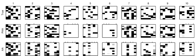
Figure 4: The figure compares the solutions achieved by standard archetypal analysis and the probabilistic formulation on binary observations. Each column is an independent trial, and each algorithm has been run 10 times to find the best archetypal profiles. The archetypal profiles are binarized, and matched with the true archetypes using minimum Jaccard distance. If a unique match is found then the corresponding archetypal profile is displayed. Otherwise they are left blank, and tagged by a circle. We observe that the probabilistic approach has been able to match archetypes better than the standard solution.

Nonnegative matrix factorization and extensions:

Non-negative matrix factorization (NMF) decomposes a non-negative matrix $\textbf{X}\in\mathbb{R}_{+}^{M\times N}$ in two non-negative matrices $\textbf{Z}\in\mathbb{R}_{+}^{M\times K}$ and $\textbf{H}\in\mathbb{R}_{+}^{K\times N}$ such that $\textbf{X}\approx\textbf{Z}\textbf{H}$. (Lee and Seung, 1999) applied the celebrated multiplicative update rule to solve this problem, and proved that such update rules lead to monotonic decrease in the cost function using the concept of majorization-minimization (Lee and Seung, 2000). Non-negative matrix factorization has been extended to convex non-negative matrix factorization (C-NMF (Ding et al, 2010)) where X is not restricted to be non-negative, and Z is expressed in terms of the X itself as $\textbf{Z}=\textbf{X}\textbf{W}$, where W is again a non-negative matrix. The motivation for this modification emerges from its similarity to clustering, and C-NMF has been solved using multiplicative update rule as well.

To simulate the exact clustering scenario, however, H is required to be binary (hard clustering) or at least column stochastic (fuzzy clustering). This leads to a more difficult optimization problem, and is usually solved by proxy constraint $\textbf{H}^{\top}\textbf{H}=\textbf{I}$ (Ding et al, 2006). Several other alternatives have also been proposed for tackling the stochasticity constraints, e.g., by enforcing it after each iteration (Mørup and Hansen, 2012), or by employing a gradient-dependent Lagrangian multiplier (Yang and Oja, 2012). However, both these approaches are prone to finding local minima.

Figure 5: The figure compares the solutions achieved by standard archetypal analysis and the probabilistic formulation on count observations. Each column is an independent trial, and each algorithm has been run 10 times to find the best archetypal profiles. The archetypal profiles are matched with the true archetypes using minimum $l_{1}$ distance. If a unique match is found then the corresponding archetypal profile is displayed. Otherwise they are left blank, and tagged by a circle. We observe that the probabilistic approach has been able to match archetypes better than the standard solution.

5 Simulation

In this section, we provide some simple examples showing the difference between probabilistic and standard archetypal analysis solutions. Since we generate data following the true probabilistic model, it is expected that the solution provided by PAA would be more appropriate compared to the standard AA solution. Therefore, the purpose of this section is to perform sanity check, and provide insight. Notice that generating observations with known archetypes is not straight forward, since $\boldsymbol{\Theta}$ depends on X.

Binary observations:

We generate $K=6$ binary archetypes in $d=10$ dimensions by sampling $\eta_{ik}\sim\mathrm{Bernoulli}(p_{s})$, where $\boldsymbol{\eta}_{k}$ is an archetype, and $p_{s}=0.3$ is the probability of success. Given the archetypes, we generate $n=100$ observations as $\textbf{x}_{i}\sim\mathrm{Bernoulli}(\textbf{E}\textbf{h}_{i})$, where $\textbf{E}=[\boldsymbol{\eta}_{1},\ldots,\boldsymbol{\eta}_{k}]$, and each $\textbf{h}_{i}$ is a stochastic vector sampled from $\mathrm{Dir}(\alpha)$. To ensure that $\boldsymbol{\eta}$’s are archetypes, we maintain more observations around $\boldsymbol{\eta}_{k}$s by choosing $\alpha=0.4$. We find archetypal profiles using both PAA and standard AA, and then binarize them so that they can be matched to the original archetypes using minimum Jaccard distance. We report the results in Fig. 4. We observe that PAA has been more successful in finding the true archetypes.

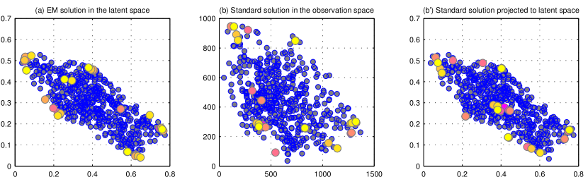
Figure 6: The figure compares the solutions achieved by standard archetypal analysis and probabilistic archetypal analysis on term-frequency observations. Each observation vector of the term-frequency matrix is generated from a probability vector within a clear convex hull (a). The probability vectors are generated such there are 5 archetypes. However, this structure is lost in the term-frequency values due to arbitrary number of occurrences in each term-frequency vector (b). The standard AA applied to term-frequency matrix thus, does not capture the true archetypes (b’).

Poisson observations:

We generate $K=6$ count archetypes in $d=12$ dimensions with one minimal archetype ($\eta_{ik}=0$), one maximal archetype $\eta_{ik}\sim\mathrm{Unif}\{1,\ldots,10\}$, and rest of the archetpyes with two nonzero entries $\eta_{ik}\ \sim\mathrm{Unif}\{1,\ldots,10\}$. Given the archetypes, we generate $n=500$ observations as $\textbf{x}_{i}\sim\mathrm{Poisson}(\textbf{E}\textbf{h}_{i})$, where $\textbf{E}=[\boldsymbol{\eta}_{1},\ldots,\boldsymbol{\eta}_{k}]$, and each $\textbf{h}_{i}$ is a stochastic vector sampled from $\mathrm{Dir}(\alpha)$. To ensure that $\boldsymbol{\eta}$’s are archetypes, we maintain more observations around $\boldsymbol{\eta}_{k}$s by choosing $\alpha=0.4$. We find archetypal profiles using both PAA and standard AA, and match them to the original archetypes using minimum $l_{1}$ distance. We report the results in Fig. 5. We observe that PAA has been more successful in finding the true archetypes.

Term-frequency observations:

We generate $K=5$ archetypes on $d=3$ dimensional probability simplex by choosing $K$ equidistant points $\textbf{p}_{k}$ on a circle in the simplex. Given the archetypes, we generate $n=500$ observations as $\textbf{x}_{i}\sim\mathrm{Mult}(n_{i},\textbf{P}\textbf{h}_{i})$, where $\textbf{P}=[\boldsymbol{p}_{1},\ldots,\boldsymbol{p}_{k}]$, and each $\textbf{h}_{i}$ is a stochastic vector sampled from $\mathrm{Dir}(\alpha)$. To ensure that p’s are archetypes, we maintain more observations around them by choosing $\alpha=0.5$. We deliberately choose an arbitrary number of occurrences $n_{i}\sim\mathrm{Uniform}[1000,2000]$ for each observation: this disrupts the true convex hull structure in the term-frequency observations. We present 10 random runs on these observations for both PAA and standard AA in Fig. 6. We observe that PAA finds the effective archetypes, with occasional local minima. However, standard AA performs poorly since it finds the appropriate archetypes in the term-frequency space, which are different when projected back on the simplex.

6 Simplex visualizations

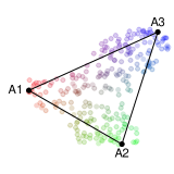
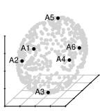
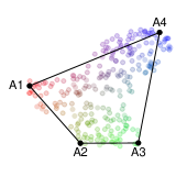
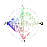
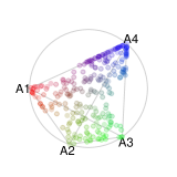
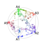
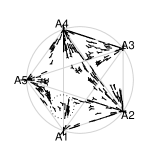
Figure 7: Simplex visualizations with extensions for different illustrative data sets and AA solutions: figures (a-c) and (d-f) illustrate color-coded points based on the deviance; figures (g-i) illustrate the ordering of the vertices according to the distances of the archetypes in the original space; and figures (j-l) illustrate the enhancement of the plot to show the composition of observations.

The column stochasticity of H allows a principled visualization scheme of archetypal analysis solution, referred to as simplex visualization. We discuss certain aspects and enhancements of this approach, and show how it can be utilized to better understand the inferred archetypes.

The stochastic nature of $\textbf{h}_{n}$ implies that $\textbf{Z}\textbf{h}_{n}$ exists on a standard $(K-1)$-simplex with the $K$ archetypes Z as the corners, and $\textbf{h}_{n}$ as the coordinate with respect to these corners (see Figure 1b for an illustration). A standard simplex can be projected to two dimensions via a skew orthogonal projection, where all the vertices of the simplex are shown on a circle connected by edges. The individual factors $\textbf{h}_{n}$ can be then projected into this circle. Figure 7 illustrates this principle with the simple data set already used in Figure 1: (a, b) for the three archetypes solution; (g, h) for the four archetypes solution; (j, k) for the five archetypes solution. Color coding is used in the six figures to show the relation between the original observation $\textbf{x}_{n}$ and its projection $\textbf{h}_{n}$. The visualization with three archetypes is known as ternary plot (see, e.g., Friendly, 2000), and has been used by Cutler and Breiman (1994). The extension to more than three archetypes has also been used (e.g., Bauckhage and Thurau, 2009; Eugster and Leisch, 2013). However, a formal study of this visualization scheme, to the best of our knowledge, remains to be explored. In the following, we present three enhancements of this basic visualization to either highlight certain characteristics of an archetypal analysis solution or to overcome consequences of the one-to-many projection.

In AA, observations which lie outside the approximated convex hull are projected onto its boundary. Figures 7a and b show a simple scenario where these observations are projected onto the corresponding edges. Figures 7d and e show an extreme case of this characteristic: the observations lie on a three-dimensional sphere, and therefore the computed archetypes span a space, which is completely empty. In the corresponding simplex visualization, however, this aspect of the solution is not visible at all. We propose to visualize the ‘deviance’ $D(\textbf{x}_{n})=2(\log{p(\textbf{x}_{n}|\theta_{n})}-\log{p(\textbf{x}_{n}|\textbf{Z}\textbf{h}_{n})})$ where $\theta_{n}$ is the maximum likelihood estimate of $\textbf{x}_{n}$, as colors of the points. In case of normal observation model the deviance reduces to the residual sum of squares. Figure 7c shows the corresponding simplex visualization with deviance for the three archetypes solution. The color scheme is from blue to white, with blue implying zero deviance and the lighter the color, the higher the deviance. We can now identify how well the original observations have been approximated by the archetypes, and if they are inside the convex hull. This extension is even more insightful in case of the sphere example. In the corresponding simplex visualization in Figure 7f, we can now clearly see that almost all observations are outside the approximated convex hull; only around the corners the deviance is near to zero.

The basic simplex visualization arranges the vertices, which represents the archetypes, equidistant on the circle. The archetypes in the original space, however, are usually not equidistant to each other. Figure 7g and h illustrate this discrepancy: archetype A2, for example, is much nearer to A3 than A4; in the simplex visualization, however, both are in the same distance. We propose to order the vertices on the circle according to their distances in the original space. This means, we first have to determine an optimal order of the vertices, and then divide the 360^∘ of the circle in relation to the original pairwise distances of the determined neighbor vertices. Here, we solve a Traveling Salesman Problem to get an optimal cyclic order (solved by using, for example, Hahsler and Hornik, 2007); and then simply divide the circle proportional to the original distances. Figure 7i shows the result: it is now clearly visible that A2 and A3 are much nearer to each other than A3 and A4.

Another problem of the simplex visualization with more than three archetypes is the non-uniqueness. As a result two projections $\textbf{h}_{n1}$ and $\textbf{h}_{n2}$ can be close to each other even though they are composed of different archetypes. This goes against one’s intuition in judging which archetypes the observations belong to. For example, the observations inside the dashed circle in Figure 7k. We get the idea that these observations are basically composed by A1, A2, A5, and/or A4—but we do not get the exact compositions. We therefore propose to show ‘whiskers’, which point in the direction of the composing archetypes, Figure 7l shows the corresponding visualization. We can now easily see the composition of the observations inside the dashed circle: the observations on the right side of the line are composed by A1 and A4; the observations on the left side of the line are composed by A1, A2, A5; and the left-most observation is composed by A1, A5. We vary the length of the ‘whiskers’ according to the coefficients $\textbf{h}_{n}$; the longer the whisker the closer the observation is to the archetype the whisker points toward.

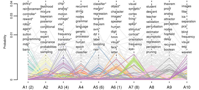
Figure 8: The probability of the words available in the NIPS corpus for each of the ten archetypal profiles. The number in parentheses refers to the corresponding archetype in (Mørup and Hansen, 2012). The colored lines show the ten most prominent words (after removing the “common” words), * indicates which words appear in both solutions. More information in Section 7.1.

7 Applications

In each application below (except the first one), we run PAA with $2\mbox{--}15$ archetypes, $10$ trials with random initializations for each number of archetypes, and choose the solution from the trials with maximum likelihoods according to the “elbow criterion”. The elbow criterion is a simple heuristic. Due to the fact that with each additional archetype $\mathbb{LL}$ increases, one can compute solutions with successively increasing number of archetypes, plot $\mathbb{LL}$ against the number or archetypes, and visually pick the solution after which the jump of $\mathbb{LL}$ “is only marginal” (i.e., the elbow). This solution is ad hoc and subjective—but widely used: “Statistical folklore has it that the location of such an ’elbow’ indicates the appropriate number of clusters” (Tibshirani and Walther, 2005).

7.1 Multinomial observations: NIPS bag-of-words

We use a data set already explored by (Mørup and Hansen, 2012) for archetypal analysis, to qualitatively evaluate the solution provided by PAA with multinomial observation model. We analyze the NIPS bag-of-words corpus consisting of $N=1500$ documents and $M=12419$ words (available from (Bache and Lichman, 2013)) and compute $K=10$ document archetypes, as in (Mørup and Hansen, 2012). We use the term-frequencies as features without normalizing them by the document frequency as in (Mørup and Hansen, 2012) to adhere to the generative nature of the documents. Figure 8 shows the probability for each word available in the corpus to be generated by the corresponding archetype (Z). Following (Mørup and Hansen, 2012), we highlight the ten most prominent terms after ignoring the “common” terms, which are present in each of the archetypes in the first 3000 words (with probability values $>10^{-4}$). We can observe that the prominent terms in a particular archetype have low probability in all the other archetypes: this agrees with our understanding of an archetype. Overall our algorithm finds a similar solution to Mørup and Hansen (2012)—one difference, however, protrudes: we find a “Bayesian Paradigm” archetype (A2), which Mørup and Hansen (2012) finds as a $k$-means prototype. But, to the best of our knowledge a “Bayesian Paradigm” archetypal document can make sense in a NIPS corpus.

7.2 Bernoulli observations: Austrian national guest survey

	A1	A3	A5	A4	A6	A2
Alpine Ski	1.00 (1)	1.00 (1)	1.00 (1)	1.00 (1)	0.00 (0)	0.00 (0)
Tour Ski	0.41 (1)	0.00 (0)	0.00 (0)	0.00 (0)	0.00 (0)	0.00 (0)
Snowboard	0.00 (0)	0.00 (0)	0.00 (0)	0.59 (1)	0.00 (0)	0.00 (0)
Cross Country	0.75 (1)	0.00 (0)	0.00 (0)	0.00 (0)	0.00 (0)	0.00 (0)
Ice Skating	0.60 (1)	0.00 (0)	0.00 (0)	0.00 (0)	0.00 (0)	0.00 (0)
Sledge	1.00 (1)	0.00 (0)	0.00 (0)	0.00 (0)	0.00 (0)	0.00 (0)
Tennis	0.15 (0)	0.00 (0)	0.00 (0)	0.00 (0)	0.00 (0)	0.20 (0)
Riding	0.00 (0)	0.00 (0)	0.00 (0)	0.00 (0)	0.00 (0)	0.08 (0)
Pool Sauna	0.96 (1)	0.00 (0)	0.37 (0)	1.00 (1)	0.82 (1)	0.11 (0)
Spa	0.22 (0)	0.00 (0)	0.00 (0)	0.00 (0)	0.79 (1)	0.00 (0)
Hiking	0.95 (1)	0.00 (0)	0.00 (0)	0.00 (0)	1.00 (1)	0.18 (0)
Walk	1.00 (1)	0.00 (0)	1.00 (1)	0.00 (0)	1.00 (1)	1.00 (1)
Excursion (org)	0.29 (0)	0.00 (0)	0.00 (0)	0.00 (0)	0.00 (0)	0.41 (1)
Excursion (ind)	0.81 (1)	0.00 (0)	0.00 (0)	0.00 (0)	0.94 (1)	1.00 (1)
Relax	0.99 (1)	0.00 (0)	1.00 (1)	1.00 (1)	1.00 (1)	0.81 (0)
Dinner	0.82 (1)	0.53 (0)	0.86 (1)	0.02 (0)	0.00 (0)	1.00 (1)
Shopping	1.00 (1)	0.00 (0)	1.00 (1)	0.01 (0)	0.33 (0)	1.00 (1)
Concert	0.00 (0)	0.00 (0)	0.00 (0)	0.00 (0)	0.00 (0)	0.29 (1)
Sightseeing	0.66 (1)	0.00 (0)	0.00 (0)	0.00 (0)	0.66 (1)	1.00 (1)
Heimat	0.58 (1)	0.00 (0)	0.00 (0)	0.00 (0)	0.00 (0)	0.00 (0)
Museum	0.00 (0)	0.00 (0)	0.00 (0)	0.00 (0)	0.00 (0)	1.00 (1)
Theater	0.00 (0)	0.00 (0)	0.00 (0)	0.00 (0)	0.00 (0)	0.30 (1)
Heurigen	0.00 (0)	0.00 (0)	0.00 (0)	0.00 (0)	0.00 (0)	0.45 (0)
Local Event	0.99 (1)	0.00 (0)	0.00 (0)	0.00 (0)	0.00 (0)	0.10 (0)
Disco	0.68 (1)	0.00 (0)	0.00 (0)	1.00 (1)	0.00 (0)	0.08 (0)
Interpretation	Maximal	Minimal	Basic		Non-Sportive
of the archetypes			Traditional	Modern	Wellness	Cultural

Table 2: The six archetypal profiles for the winter tourists example. The corresponding archetypal observations are shown in parentheses. For more information, see Section 7.2.

Analyzing binary survey data is of utmost importance in social science and marketing research. A binary questionnaire is often preferred over an ordinal multi-category format, since the former is quicker and easier, whereas both are equally reliable, and the managerial implications derived from them do not substantially differ (Dolnicar et al, 2011). In this application, we analyze binary survey data from the Austrian National Guest Survey conducted in the winter season of 1997. The goal is to identify archetypal winter tourists, which may facilitate developing and targeting specific advertising materials. The data consists of $2958$ tourists. Each tourist answers $25$ binary questions on whether he/she is engaged in a certain winter activity (e.g., alpine skiing, relaxing, or shopping; see row description of Table 2 for the complete list). In addition, a number of descriptive variables are available (e.g., the age and gender of the tourist).

Here we present the six archetypes solution. Table 2 lists the archetypal profiles (i.e., the probability of positive response) and, in parentheses, the corresponding archetypal observations (with maximum $w$ value). Archetype A1 is the maximal winter tourist who is engaged in nearly every sportive and wellness activity with high probability. Archetype A3, on the other hand, is the minimal winter tourist who is only engaged in alpine skiing and having dinner. Both archetypes A5 and A4 are engaged in the basic Austrian winter activities (alpine skiing, indoor swimming, and relaxing). In addition, A5 is engaged in traditional activities (dinner and shopping), whereas A4 is engaged in more modern activities (snowboarding and going to a disco). Finally, A6 and A2 are the non-sportive archetypes. A6 is engaged in wellness activities and A2 with cultural activities. Note that important engagements of the archetypes are missed if one only looks at the archetypal observations rather than the archetypal profiles; e.g., the possible engagement of A2 in hiking. We can now utilize the factors H for each of the tourists to learn their relations to the archetypal winter tourist profiles. This allows us, for example, to target very specific advertising material to tourists for the next winter season.

To get further insight into the archetypes we explore the simplex visualization. Figure 9 shows four simplex visualizations with the archetypes arranged according to their distance in the original space and the composition of the winter tourists indicated by corresponding whiskers. Figure 9a shows the model deviance normalized from 0 (blue) to 1 (white). We can observe that the tourists mainly explained by the Minimal (A3), Modern (A4), Traditional (A5), and/or Wellness (A6) archetypes are well represented (darker blue). The Maximal (A1) archetype seems to be an outlier, there are only a few observations near to this archetype, and the deviance is higher for these observations. Figures 9b-d highlight tourists’ answers to certain questions (yes/black and no/gray). Figure 9b shows whether a tourist does snowboarding or not. We can see that most of the tourists who do snowboarding are arranged around and point towards A4, which we interpreted as the Modern archetype. In Figure 9c we highlight whether a tourist visits a museum or not. Here, most of the tourists who go there are arranged around A2, which we interpreted as the Cultural archetype. Figure 9d shows an activity which does not discriminate between archetypes—nearly all tourists do shopping, and no specific pattern is visible in this visualization.

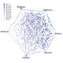
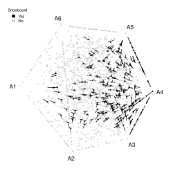
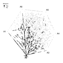
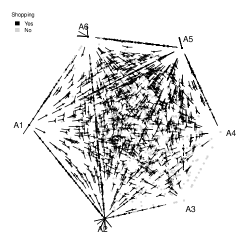
Figure 9: Simplex visualizations for the the Austrian national guest survey example. The archetypes are arranged according to their distance in the original space and the composition of the winter tourists is indicated by corresponding whiskers. Figure (a) shows the model deviance normalized from 0 (blue) to 1 (white); figures (b-d) highlight tourists’ answers to certain questions (yes/black and no/gray). See Section 7.2 for detailed interpretations.

7.3 Poisson observations: Disasters worldwide from 1900–2008

In this application, the goal is to identify archetypal countries that are affected by a particular disaster or a combination of disasters. This may be helpful in emergency management and to facilitate devising disaster prevention plans for countries based on prevention plans designed for the archetypal disaster-affected countries. We compile a dataset with disaster counts for $227$ countries (historical and present countries) in $15$ categories from the EM-DAT database (EM-DAT, 2013). This is a global database on natural and technological disasters between 1900–present. The criteria to be a disaster are: ten or more reported casualty; hundred or more people reported affected; declaration of a state of emergency; or call for international assistance. The list of disaster categories is provided in Figure 10; see the EM-DAT website for specific details.

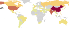
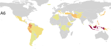
Figure 10: The seven archetypal profiles for the disaster example: (top left) Plot of archetypal profiles ($\%$ of maximum value); (world maps) Factors H for each archetype. Disasters: complex disasters (CD), drought (DR), earthquake (EQ), epidemic (EP), extreme temperature (ET), flood (FL), industrial accident (IA), insect infestation (II), mass movement dry (MD), mass movement wet (MW), miscellaneous accident (MA), storm (ST), transport accident (TA), volcano (VO), and wildfire (WF). See Section 7.3 for details.

We present the seven archetypes solution; Figure 10 shows a summary. There are two minimal profiles A1 and A7 with small differences in the categories extreme temperature/flood and storm. A1 can be considered as the archetypal profile for safe country where the corresponding archetypal observations include Malta and the Cayman Islands (other close observations are the Nordic countries). Archetype A5 is the maximal archetypal profile with counts in every category, and the corresponding archetypal observations include China and United States. This can be expected from the size and population of the countries; China (third and first), USA (fourth and third). Other countries with high factor H for this archetypal profile are India (seventh and second), and Russia (first and ninth). A3 and A4 are the archetypes that are affected by drought and epidemic; where A3 additionally has a high insect infestation count. A2 is the archetype that is susceptible to complex disasters (where neither nature nor human is the definitive cause) only, whereas A6 has high counts in the categories earthquake, flood, mass movement wet, and volcano. Here the archetypal countries include Indonesia and Colombia.

Figure 11 shows two simplex visualizations with the archetypes arranged according to their distance in the original space. This arrangement shows that A1 is very near to A7, which is in line with the archetypal profiles plot shown in Figure 10. Figure 11a shows the model deviance normalized from 0 (blue) to 1 (white). We can see that A2, A3, A4, A5 and A6 are basically outliers with only one or very few observations are around them. Most of the observations with low deviance are near A1 and A7. Figure 11b highlights the countries’ insect infestation (the higher the count the bigger the point). We can see a clear pattern around A3, with Niger (NE), Chad (TD), Mali (ML), Senegal (SN), Sudan (SD), Ethiopia (ET), Gambia (GM), Mauritania (MR), and Morocco (MA) as the top countries affected by insect infestation.

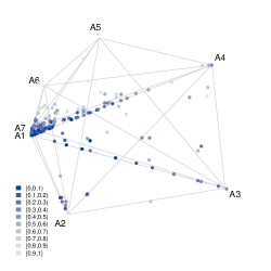
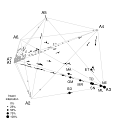
Figure 11: Simplex visualizations for the disasters example: The archetypes are arranged according to their distance in the original space. Figure (a)  shows the model deviance normalized from 0 (blue) to 1 (white); Figure (b) shows the projected countries scaled according to the number of Insect infestations (ISO2 country codes for the top countries). See Section 7.3 for detailed interpretations.

8 Discussion

Archetypal analysis expresses observations as composition of extreme values, or archetypes. Archetypes can be thought of as ideal or pure characteristics, and the goal of archetypal analysis is to find these characteristics, and to explain the available observations as combination of these characteristics. The standard formulation of archetypal analysis was suggested by Cutler and Breiman and is based on finding the approximate convex hull of the observations. Over the last decade this approach has been extensively used by researchers. But, their applications have mostly been limited to real valued observations. In this paper, we have proposed a probabilistic formulation of archetypal analysis, which enjoys several crucial advantages over the geometric approach, including but not limited to the extension to other observation models: Bernoulli, Poisson and multinomial. We have achieved this by approximating the convex hull in the parameter space under a suitable observation model. Our contribution lies in formally extending the standard AA framework, suggesting efficient optimization tools based on majorization-minimization method, and demonstrating the applicability of such approaches in practical applications. We have also suggested improvements of the standard simplex visualization tool to better show the intricacies in the archetypal analysis solution.

The probabilistic framework provides further advantages that remains to be explored in its entirety. For example, it provides a theoretically sound approach for choosing the number of archetypes. This can be done by imposing appropriate prior over W and H matrices, such as a symmetric Dirichlet distribution with coefficient $<1$. The prior can be used to effectively shrink and expand the convex hull to fit the observations. Since the Dirichlet distribution is a natural prior for multinomial distribution, this solution can be approximated relatively easily using variational Bayes’ approach, and initial results show that this is indeed and effective approach for choosing the number of archetypes. However, this becomes a slightly trickier problem when applied to other observation models, such as normal and Poisson. We are currently working on suitable methods to solve the related optimization problems efficiently.

Another potential extension of the probabilistic framework is to tackle ordinal or Likert scale variables. Since ordinal variables lack additivity, they must be addressed through a probabilistic set-up with suitable observation model. Given the fact that survey data is often in Likert scale, archetypal analysis of such observations can have a large impact on social science and marketing: describe, e.g., the personality of consumers in terms of the personality of the most “extreme”, i.e., archetypal, consumers (using, e.g., the Likert scaled items defined by the Big Five Inventory). We believe that these suggested improvements will make archetypal analysis more robust and accessible to non-scientific users.

Acknowledgement:

The calculations presented above were performed using computer resources within the Aalto University School of Science “Science-IT” project.

Appendix A Update rules for multinomial observations

For simplicity, let us consider the following problem of finding, $\textbf{X}=\textbf{H}\textbf{W}\textbf{P}$ where X is now $n\times m$ matrix instead of $m\times n$ matrix in the earlier sections. Then this problem can be viewed as given a document choose a topic following H, then given a topic choose a document (subtopic) following W, and finally given a document (subtopic) choose a word following P. Let $\textbf{R}^{jk}_{il}$ be the indicator variable for selecting topic $j$ and document (subtopic) $k$. Then the log-likelihood of the observations X is given by

$$\mathbb{LL}\left(\textbf{X}|\textbf{H},\textbf{W},\textbf{P},\textbf{R}\right) =\sum_{il}\textbf{X}_{il}\log\left(\prod_{jk}\textbf{H}_{ij}\textbf{W}_{jk}\textbf{P}_{kl}\right)^{z^{jk}_{il}}+C_{0}$$

$$=\sum_{ijkl}\textbf{X}_{il}{z^{jk}_{il}}\log\left(\textbf{H}_{ij}\textbf{W}_{jk}\textbf{P}_{kl}\right)+C_{0}$$

At each expectation step we need to evaluate,

$$\mathbb{E}\left[z^{jk}_{il}|\textbf{X},\textbf{H},\textbf{W},\textbf{P}\right]=\mathrm{P}(z^{jk}_{ik}=1|\textbf{X},\textbf{H},\textbf{W},\textbf{P})=\frac{\textbf{H}_{ij}\textbf{W}_{jk}\textbf{P}_{kl}}{(\textbf{H}\textbf{W}\textbf{P})_{il}}$$

then the maximization step gives us the final update equation.

Appendix B Update rule for Poisson observations

We show that the update rule discussed in the article leads to monotonic decrease in the cost function using majorization-minimization. We reformulate the problem as

$$\min_{\textbf{W},\textbf{H}\geq 0} \sum_{ij}\left[-\textbf{X}_{ij}\log\sum_{mn}\boldsymbol{\Lambda}_{im}\textbf{W}_{mn}\textbf{H}_{nj}+\sum_{mn}\boldsymbol{\Lambda}_{im}\textbf{W}_{mn}\textbf{H}_{nj}\right]$$

$$\qquad\qquad+\lambda\sum_{j}\left(-\log\sum_{n}\textbf{H}_{nj}+\sum_{n}\textbf{H}_{nj}\right)+\lambda\sum_{n}\left(-\log\sum_{m}\textbf{W}_{mn}+\sum_{m}\textbf{W}_{mn}\right)$$

where $\lambda>0$ is a suitably large regularization parameter to enforce the equality constraint in a relaxed fashion.

Given $\phi_{inj}=\frac{\sum_{m}\boldsymbol{\Lambda}_{im}\textbf{W}_{mn}\textbf{H}_{nj}}{\sum_{mn}\boldsymbol{\Lambda}_{im}\textbf{W}_{mn}\textbf{H}_{nj}}$, and $\psi_{nj}=\frac{\textbf{H}_{nj}}{\sum_{n}\textbf{H}_{nj}}$, we can construct the auxiliary function for H as,

$$\sum_{ij}\left[-\textbf{X}_{ij}\log\sum_{mn}\boldsymbol{\Lambda}_{im}\textbf{W}_{mn}\tilde{\textbf{H}}_{nj}+\sum_{mn}\boldsymbol{\Lambda}_{im}\textbf{W}_{mn}\tilde{\textbf{H}}_{nj}\right]$$

$$\qquad+\lambda\sum_{j}\left(-\log\sum_{n}\tilde{\textbf{H}}_{nj}+\sum_{n}\tilde{\textbf{H}}_{nj}\right)$$

$$= \sum_{ij}\left[-\textbf{X}_{ij}\log\sum_{n}\frac{\phi_{inj}}{\phi_{inj}}\sum_{m}\boldsymbol{\Lambda}_{im}\textbf{W}_{mn}\tilde{\textbf{H}}_{nj}+\sum_{mn}\boldsymbol{\Lambda}_{im}\textbf{W}_{mn}\tilde{\textbf{H}}_{nj}\right]$$

$$\qquad+\lambda\sum_{j}\left(-\log\sum_{n}\frac{\psi_{nj}}{\psi_{nj}}\tilde{\textbf{H}}_{nj}+\sum_{n}\tilde{\textbf{H}}_{nj}\right)$$

$$\leq \sum_{ij}\left[-\textbf{X}_{ij}\sum_{n}\phi_{inj}\log\frac{\sum_{m}\boldsymbol{\Lambda}_{im}\textbf{W}_{mn}\tilde{\textbf{H}}_{nj}}{\phi_{inj}}+\sum_{mn}\boldsymbol{\Lambda}_{im}\textbf{W}_{mn}\tilde{\textbf{H}}_{nj}\right]$$

$$\qquad+\lambda\left(\sum_{nj}-\psi_{nj}\log\frac{\tilde{\textbf{H}}_{nj}}{\psi_{nj}}+\sum_{nj}\tilde{\textbf{H}}_{nj}\right)$$

$$= \sum_{ij}\left[-\textbf{X}_{ij}\sum_{n}\phi_{inj}\log\tilde{\textbf{H}}_{nj}+\sum_{mn}\boldsymbol{\Lambda}_{im}\textbf{W}_{mn}\tilde{\textbf{H}}_{nj}\right]$$

$$\qquad+\lambda\left(\sum_{nj}-\psi_{nj}\log\tilde{\textbf{H}}_{nj}+\sum_{nj}\tilde{\textbf{H}}_{nj}\right)+C$$

The derivative is then given by

$$\frac{\partial\cdot}{\partial\tilde{\textbf{H}}_{nj}}= -\frac{\sum_{i}\textbf{X}_{ij}\phi_{inj}}{\tilde{\textbf{H}}_{nj}}+\sum_{im}\boldsymbol{\Lambda}_{im}\textbf{W}_{mn}-\frac{\lambda\psi_{nj}}{\tilde{\textbf{H}}_{nj}}+\lambda$$

$$= -\frac{\textbf{H}_{nj}}{\tilde{\textbf{H}}_{nj}}\left(\sum_{i}\frac{\textbf{X}_{ij}\sum_{m}\boldsymbol{\Lambda}_{im}\textbf{W}_{mn}}{\sum_{mn}\boldsymbol{\Lambda}_{im}\textbf{W}_{mn}\textbf{H}_{nj}}+\frac{\lambda}{\sum_{n}\textbf{H}_{nj}}\right)+\left(\sum_{im}\boldsymbol{\Lambda}_{im}\textbf{W}_{mn}+\lambda\right)$$

Equating the derivative to zero provides the update rule.

Given $\phi_{imnj}=\frac{\boldsymbol{\Lambda}_{im}\textbf{W}_{mn}\textbf{H}_{nj}}{\sum_{mn}\boldsymbol{\Lambda}_{im}\textbf{W}_{mn}\textbf{H}_{nj}}$, and $\psi_{mn}=\frac{\textbf{W}_{mn}}{\sum_{m}\textbf{W}_{mn}}$, we can construct the auxiliary function for W as,

$$\sum_{ij}\left[-\textbf{X}_{ij}\log\sum_{mn}\boldsymbol{\Lambda}_{im}\tilde{\textbf{W}}_{mn}\textbf{H}_{nj}+\sum_{mn}\boldsymbol{\Lambda}_{im}\tilde{\textbf{W}}_{mn}\textbf{H}_{nj}\right]$$

$$\qquad+\lambda\sum_{n}\left(-\log\sum_{m}\tilde{\textbf{W}}_{mn}+\sum_{m}\tilde{\textbf{W}}_{mn}\right)$$

$$= \sum_{ij}\left[-\textbf{X}_{ij}\log\sum_{mn}\frac{\phi_{imnj}}{\phi_{imnj}}\boldsymbol{\Lambda}_{im}\tilde{\textbf{W}}_{mn}\textbf{H}_{nj}+\sum_{mn}\boldsymbol{\Lambda}_{im}\tilde{\textbf{W}}_{mn}\textbf{H}_{nj}\right]$$

$$\qquad+\lambda\sum_{n}\left(-\log\sum_{m}\frac{\psi_{mn}}{\psi_{mn}}\tilde{\textbf{W}}_{mn}+\sum_{m}\tilde{\textbf{W}}_{mn}\right)$$

$$\leq \sum_{ij}\left[-\textbf{X}_{ij}\sum_{mn}\phi_{imnj}\log\frac{\boldsymbol{\Lambda}_{im}\tilde{\textbf{W}}_{mn}\textbf{H}_{nj}}{\phi_{imnj}}+\sum_{mn}\boldsymbol{\Lambda}_{im}\tilde{\textbf{W}}_{mn}\textbf{H}_{nj}\right]$$

$$\qquad+\lambda\left(\sum_{mn}-\psi_{mn}\log\frac{\tilde{\textbf{W}}_{mn}}{\psi_{mn}}+\sum_{mn}\tilde{\textbf{W}}_{mn}\right)$$

$$= \sum_{ij}\left[-\textbf{X}_{ij}\sum_{mn}\phi_{imnj}\log\tilde{\textbf{W}}_{mn}+\sum_{mn}\boldsymbol{\Lambda}_{im}\tilde{\textbf{W}}_{mn}\textbf{H}_{nj}\right]$$

$$\qquad+\lambda\left(\sum_{mn}-\psi_{mn}\log\tilde{\textbf{W}}_{mn}+\sum_{mn}\tilde{\textbf{W}}_{mn}\right)+C$$

The derivative is then given by

$$\frac{\partial\cdot}{\partial\tilde{\textbf{W}}_{mn}}= -\frac{\sum_{ij}\textbf{X}_{ij}\phi_{imnj}}{\tilde{\textbf{W}}_{mn}}+\sum_{ij}\boldsymbol{\Lambda}_{im}\textbf{H}_{nj}-\frac{\lambda\psi_{mn}}{\tilde{\textbf{W}}_{mn}}+\lambda$$

$$= -\frac{\textbf{W}_{mn}}{\tilde{\textbf{W}}_{mn}}\left(\sum_{ij}\frac{\textbf{X}_{ij}\boldsymbol{\Lambda}_{im}\textbf{H}_{nj}}{\sum_{mn}\boldsymbol{\Lambda}_{im}\textbf{W}_{mn}\textbf{H}_{nj}}+\frac{\lambda}{\sum_{m}\textbf{W}_{mn}}\right)+\left(\sum_{ij}\boldsymbol{\Lambda}_{im}\textbf{H}_{nj}+\lambda\right)$$

Equating the derivative to zero provides the update rule.

Appendix C Update rule for Bernoulli observations

Since the cost function consists of two similar terms, we show how to establish the auxiliary function for one of them.

For H we have, $\phi_{inj}=\frac{\sum_{m}\textbf{P}_{im}\textbf{W}_{mn}\textbf{H}_{nj}}{\sum_{mn}\textbf{P}_{im}\textbf{W}_{mn}\textbf{H}_{nj}}$, and $\sum_{n}\phi_{inj}=1$, then

$$\sum_{ij}\left[-\textbf{X}_{ij}\log(\textbf{P}\textbf{W}\tilde{\textbf{H}})_{ij}\right]$$

$$= \sum_{ij}\left[-\textbf{X}_{ij}\log\sum_{mn}\textbf{P}_{im}\textbf{W}_{mn}\tilde{\textbf{H}}_{nj}\right]$$

$$= \sum_{ij}\left[-\textbf{X}_{ij}\log\sum_{n}\frac{\phi_{inj}}{\phi_{inj}}\sum_{m}\textbf{P}_{im}\textbf{W}_{mn}\tilde{\textbf{H}}_{nj}\right]$$

$$\leq \sum_{ij}\left[-\textbf{X}_{ij}\sum_{n}\phi_{inj}\log\frac{\sum_{m}\textbf{P}_{im}\textbf{W}_{mn}\tilde{\textbf{H}}_{nj}}{\phi_{inj}}\right]$$

$$= \sum_{ij}\left[-\textbf{X}_{ij}\sum_{n}\phi_{inj}\log\frac{\tilde{\textbf{H}}_{nj}}{\textbf{H}_{nj}}-\textbf{X}_{ij}\log\sum_{mn}\textbf{P}_{im}\textbf{W}_{mn}\textbf{H}_{nj}\right]$$

$$= \sum_{ij}\left[-\textbf{X}_{ij}\sum_{n}\phi_{inj}\log\left(\frac{\tilde{\textbf{G}}_{nj}}{\sum_{p}\tilde{\textbf{G}}_{pj}}\frac{\sum_{p}\textbf{G}_{pj}}{\textbf{G}_{nj}}\right)-\textbf{X}_{ij}\log\sum_{mn}\textbf{P}_{im}\textbf{W}_{mn}\textbf{H}_{nj}\right]$$

$$= \sum_{ij}\left[-\textbf{X}_{ij}\sum_{n}\phi_{inj}\log\frac{\tilde{\textbf{G}}_{nj}}{\textbf{G}_{nj}}+\textbf{X}_{ij}\sum_{n}\phi_{inj}\log\frac{\sum_{p}\tilde{\textbf{G}}_{pj}}{\sum_{p}\textbf{G}_{pj}}-\textbf{X}_{ij}\log\sum_{mn}\textbf{P}_{im}\textbf{W}_{mn}\textbf{H}_{nj}\right]$$

$$\leq \sum_{ij}\left[-\textbf{X}_{ij}\sum_{n}\phi_{inj}\log\frac{\tilde{\textbf{G}}_{nj}}{\textbf{G}_{nj}}+\textbf{X}_{ij}\left(\frac{\sum_{p}\tilde{\textbf{G}}_{pj}}{\sum_{p}\textbf{G}_{pj}}-1\right)-\textbf{X}_{ij}\log\sum_{mn}\textbf{P}_{im}\textbf{W}_{mn}\textbf{H}_{nj}\right]$$

Taking derivative we get,

$$\sum_{i}\left[-\textbf{X}_{ij}\phi_{inj}\frac{1}{\tilde{\textbf{G}}_{nj}}+\textbf{X}_{ij}\frac{1}{\sum_{p}\textbf{G}_{pj}}\right]$$

$$\Rightarrow \tilde{\textbf{G}}_{nj}=\frac{\sum_{p}\textbf{G}_{pj}}{\sum_{i}\textbf{X}_{ij}}\left(\sum_{i}\frac{\textbf{X}_{ij}\sum_{m}\textbf{P}_{im}\textbf{W}_{mn}\textbf{H}_{nj}}{\sum_{mn}\textbf{P}_{im}\textbf{W}_{mn}\textbf{H}_{nj}}\right)=\frac{\textbf{G}_{nj}}{\sum_{i}\textbf{X}_{ij}}\left(\sum_{i}\frac{\textbf{X}_{ij}\sum_{m}\textbf{P}_{im}\textbf{W}_{mn}}{\sum_{mn}\textbf{P}_{im}\textbf{W}_{mn}\textbf{H}_{nj}}\right)$$

For W we have, $\phi_{imnj}=\frac{\textbf{P}_{im}\textbf{W}_{mn}\textbf{H}_{nj}}{\sum_{mn}\textbf{P}_{im}\textbf{W}_{mn}\textbf{H}_{nj}}$, and $\sum_{mn}\phi_{imnj}=1$, then

$$\sum_{ij}\left[-\textbf{X}_{ij}\log(\textbf{P}\tilde{\textbf{W}}\textbf{H})_{ij}\right]$$

$$= \sum_{ij}\left[-\textbf{X}_{ij}\log\sum_{mn}\textbf{P}_{im}\tilde{\textbf{W}}_{mn}\textbf{H}_{nj}\right]$$

$$= \sum_{ij}\left[-\textbf{X}_{ij}\log\sum_{mn}\frac{\phi_{imnj}}{\phi_{imnj}}\textbf{P}_{im}\tilde{\textbf{W}}_{mn}\textbf{H}_{nj}\right]$$

$$\leq \sum_{ij}\left[-\textbf{X}_{ij}\sum_{mn}\phi_{imnj}\log\frac{\textbf{P}_{im}\tilde{\textbf{W}}_{mn}\textbf{H}_{nj}}{\phi_{imnj}}\right]$$

$$= \sum_{ij}\left[-\textbf{X}_{ij}\sum_{mn}\phi_{imnj}\log\frac{\tilde{\textbf{W}}_{mn}}{\textbf{W}_{mn}}-\textbf{X}_{ij}\log\sum_{mn}\textbf{P}_{im}\textbf{W}_{mn}\textbf{H}_{nj}\right]$$

$$= \sum_{ij}\left[-\textbf{X}_{ij}\sum_{mn}\phi_{imnj}\log\left(\frac{\tilde{\textbf{V}}_{mn}}{\sum_{p}\tilde{\textbf{V}}_{pn}}\frac{\sum_{p}\textbf{V}_{pn}}{\textbf{V}_{mn}}\right)-\textbf{X}_{ij}\log\sum_{mn}\textbf{P}_{im}\textbf{W}_{mn}\textbf{H}_{nj}\right]$$

$$= \sum_{ij}\left[-\textbf{X}_{ij}\sum_{mn}\phi_{imnj}\log\frac{\tilde{\textbf{V}}_{mn}}{\textbf{V}_{mn}}+\textbf{X}_{ij}\sum_{mn}\phi_{imnj}\log\frac{\sum_{p}\tilde{\textbf{V}}_{pn}}{\sum_{p}\textbf{V}_{pn}}-\textbf{X}_{ij}\log\sum_{mn}\textbf{P}_{im}\textbf{W}_{mn}\textbf{H}_{nj}\right]$$

$$\leq \sum_{ij}\left[-\textbf{X}_{ij}\sum_{mn}\phi_{imnj}\log\frac{\tilde{\textbf{V}}_{mn}}{\textbf{V}_{mn}}+\textbf{X}_{ij}\sum_{mn}\phi_{imnj}\left(\frac{\sum_{p}\tilde{\textbf{V}}_{pn}}{\sum_{p}\textbf{V}_{pn}}-1\right)-\textbf{X}_{ij}\log\sum_{mn}\textbf{P}_{im}\textbf{W}_{mn}\textbf{H}_{nj}\right]$$

Taking derivative we get,

$$\sum_{ij}\left[-\textbf{X}_{ij}\phi_{imnj}\frac{1}{\tilde{\textbf{V}}_{mn}}+\textbf{X}_{ij}\sum_{m}\phi_{imnj}\frac{1}{\sum_{p}\textbf{V}_{pn}}\right]$$

$$\Rightarrow \tilde{\textbf{V}}_{mn}=\frac{\sum_{p}\textbf{V}_{pn}}{\sum_{ij}\textbf{X}_{ij}\sum_{m}\phi_{imnj}}\left(\sum_{ij}\frac{\textbf{X}_{ij}\textbf{P}_{im}\textbf{W}_{mn}\textbf{H}_{nj}}{\sum_{mn}\textbf{P}_{im}\textbf{W}_{mn}\textbf{H}_{nj}}\right)$$

$$\qquad=\frac{\textbf{V}_{mn}}{\sum_{ij}\frac{\textbf{X}_{ij}\sum_{m}\textbf{P}_{im}\textbf{W}_{mn}\textbf{H}_{nj}}{\sum_{mn}\textbf{P}_{im}\textbf{W}_{mn}\textbf{H}_{nj}}}\left(\sum_{ij}\frac{\textbf{X}_{ij}\textbf{P}_{im}\textbf{H}_{nj}}{\sum_{mn}\textbf{P}_{im}\textbf{W}_{mn}\textbf{H}_{nj}}\right)$$

The update rule can be derived from these equations after including the other term with Q.

References

- Bache and Lichman (2013) Bache K, Lichman M (2013) UCI machine learning repository. URL http://archive.ics.uci.edu/ml
- Bauckhage and Thurau (2009) Bauckhage C, Thurau C (2009) Making archetypal analysis practical. In: Pattern Recognition, Lecture Notes in Computer Science, vol 5748, Springer Berlin Heidelberg, pp 272–281, DOI 10.1007/978-3-642-03798-6˙28
- Bhattacharya and Dunson (2012) Bhattacharya A, Dunson DB (2012) Simplex factor models for multivariate unordered categorical data. Journal of the American Statistical Association 107(497):362–377, DOI 10.1080/01621459.2011.646934
- Blei et al (2003) Blei DM, Ng AY, Jordan MI (2003) Latent dirichlet allocation. Journal of Machine Learning Research 3:993–1022
- Chan et al (2003) Chan BHP, Mitchell DA, Cram LE (2003) Archetypal analysis of galaxy spectra. Monthly Notices of the Royal Astronomical Society 338(3):790–795, DOI 10.1046/j.1365-8711.2003.06099.x
- Cutler and Breiman (1994) Cutler A, Breiman L (1994) Archetypal analysis. Technometrics 36(4):338–347
- Cutler and Stone (1997) Cutler A, Stone E (1997) Moving archetypes. Physica D: Nonlinear Phenomena 107(1):1–16, DOI 10.1016/S0167-2789(97)84209-1, URL http://www.sciencedirect.com/science/article/pii/S0167278997842091
- Davis and Love (2010) Davis T, Love BC (2010) Memory for category information is idealized through contrast with competing options. Psychological Science 21(2):234–242, DOI 10.1177/0956797609357712
- Ding et al (2006) Ding C, Li T, Peng W, Park H (2006) Orthogonal nonnegative matrix tri-factorizations for clustering. In: Proceedings of the 12th ACM SIGKDD International Conference on Knowledge Discovery and Data Mining, pp 126–135, DOI 10.1145/1150402.1150420
- Ding et al (2010) Ding CHQ, Li T, Jordan MI (2010) Convex and semi-nonnegative matrix factorizations. IEEE Transactions on Pattern Analysis and Machine Intelligence 32(1):45–55
- Dolnicar et al (2011) Dolnicar S, Grün B, Leisch F (2011) Quick, simple and reliable: Forced binary survey questions. International Journal of Market Research 53(2):231–252, DOI 10.2501/IJMR-53-2-231-252
- EM-DAT (2013) EM-DAT (2013) The OFDA/CRED International Disaster Database. Universite catholique de Louvain, Brussels, Belgium; http://www.emdat.net
- Eugster (2012) Eugster MJA (2012) Performance profiles based on archetypal athletes. International Journal of Performance Analysis in Sport 12(1):166–187
- Eugster and Leisch (2011) Eugster MJA, Leisch F (2011) Weighted and robust archetypal analysis. Computational Statistics and Data Analysis 55(3):1215–1225, DOI 10.1016/j.csda.2010.10.017
- Eugster and Leisch (2013) Eugster MJA, Leisch F (2013) archetypes: Archetypal Analysis. URL http://CRAN.R-project.org/package=archetypes, R package version 2.1-2
- Févotte and Idier (2011) Févotte C, Idier J (2011) Algorithms for nonnegative matrix factorization with the beta-divergence. Neural Computation 23(9):2421–2456
- Friendly (2000) Friendly M (2000) Visualizing Categorical Data. SAS Institute
- Hahsler and Hornik (2007) Hahsler M, Hornik K (2007) TSP – Infrastructure for the traveling salesperson problem. Journal of Statistical Software 23(2):1–21, URL http://www.jstatsoft.org/v23/i02/
- Hofmann (2013) Hofmann T (2013) Probabilistic latent semantic analysis. arXiv:13016705 URL http://arxiv.org/abs/1301.6705
- Lee and Seung (1999) Lee DD, Seung HS (1999) Learning the parts of objects by non-negative matrix factorization. Nature 401(6755):788–791, DOI 10.1038/44565
- Lee and Seung (2000) Lee DD, Seung HS (2000) Algorithms for non-negative matrix factorization. In: Advances in Neural Information Processing Systems 13, pp 556–562
- Li et al (2003) Li S, Louviere J, Carson R, Wang P (2003) Archetypal analysis: A new way to segment markets based on extreme individuals. In: A Celebration of Ehrenberg and Bass: Marketing Knowledge, Discoveries and Contribution. Proceedings of the ANZMAC 2003 Conference, URL http://epress.lib.uts.edu.au/research/handle/10453/2183
- Marinetti et al (2007) Marinetti S, Finesso L, Marsilio E (2007) Archetypes and principal components of an IR image sequence. Infrared Physics & Technology 49(3):272–276, DOI 10.1016/j.infrared.2006.06.017, URL http://www.sciencedirect.com/science/article/pii/S1350449506000910
- Mohamed et al (2009) Mohamed S, Heller KA, Ghahramani Z (2009) Bayesian exponential family PCA. In: Advances in Neural Information Processing Systems 21, pp 1089–1096
- Mørup and Hansen (2012) Mørup M, Hansen LK (2012) Archetypal analysis for machine learning and data mining. Neurocomputing 80:54–63, DOI 10.1016/j.neucom.2011.06.033
- do Nascimento and Dias (2005) do Nascimento JMP, Dias JMB (2005) Vertex component analysis: A fast algorithm to unmix hyperspectral data. IEEE Transactions on Geoscience and Remote Sensing 43(4):898–910, DOI 10.1109/TGRS.2005.844293
- Porzio et al (2008) Porzio GC, Ragozini G, Vistocco D (2008) On the use of archetypes as benchmarks. Applied Stochastic Models in Business and Industry 24(5):419–437, DOI 10.1002/asmb.727, URL http://onlinelibrary.wiley.com/doi/10.1002/asmb.727/abstract
- Seiler and Wohlrabe (2013) Seiler C, Wohlrabe K (2013) Archetypal scientists. Journal of Informetrics 7(2):345–356, DOI 10.1016/j.joi.2012.11.013
- Sifa and Bauckhage (2013) Sifa R, Bauckhage C (2013) Archetypical motion: Supervised game behavior learning with archetypal analysis. In: 2013 IEEE Conference on Computational Intelligence in Games (CIG), pp 1–8, DOI 10.1109/CIG.2013.6633609
- Steinley (2006) Steinley D (2006) K-means clustering: A half-century synthesis. British Journal of Mathematical and Statistical Psychology 59(1):1–34, DOI 10.1348/000711005X48266
- Stone and Cutler (1996) Stone E, Cutler A (1996) Archetypal analysis of spatio-temporal dynamics. Physica D: Nonlinear Phenomena 90(3):209–224, DOI 10.1016/0167-2789(95)00244-8
- Thøgersen et al (2013) Thøgersen JC, Mørup M, Damkiær S, Molin S, Jelsbak L (2013) Archetypal analysis of diverse pseudomonas aeruginosa transcriptomes reveals adaptation in cystic fibrosis airways. BMC Bioinformatics 14(1):279, DOI 10.1186/1471-2105-14-279, URL http://www.biomedcentral.com/1471-2105/14/279/abstract
- Thurau et al (2009) Thurau C, Kersting K, Bauckhage C (2009) Convex non-negative matrix factorization in the wild. In: Ninth IEEE International Conference on Data Mining, 2009. ICDM ’09, pp 523–532, DOI 10.1109/ICDM.2009.55
- Thurau et al (2010) Thurau C, Kersting K, Bauckhage C (2010) Yes we can: Simplex volume maximization for descriptive web-scale matrix factorization. In: Proceedings of the 19th ACM International Conference on Information and Knowledge Management, ACM, New York, NY, USA, CIKM ’10, pp 1785–1788, DOI 10.1145/1871437.1871729, URL http://doi.acm.org/10.1145/1871437.1871729
- Tibshirani and Walther (2005) Tibshirani R, Walther G (2005) Cluster validation by prediction strength. Journal of Computational and Graphical Statistics 14:511–528
- Woodbury and Clive (1974) Woodbury MA, Clive J (1974) Clinical pure types as a fuzzy partition. Journal of Cybernetics 4(3):111–121, DOI 10.1080/01969727408621685, URL http://www.tandfonline.com/doi/abs/10.1080/01969727408621685
- Xiong et al (2013) Xiong Y, Liu W, Zhao D, Tang X (2013) Face recognition via archetype hull ranking. In: 2013 IEEE International Conference on Computer Vision (ICCV), pp 585–592, DOI 10.1109/ICCV.2013.78
- Yang and Oja (2012) Yang Z, Oja E (2012) Clustering by low-rank doubly stochastic matrix decomposition. arXiv:12064676 URL http://arxiv.org/abs/1206.4676