Conditions for Conductance Quantization in Mesoscopic
Dirac Systems on the Examples of Graphene
Nanoconstrictions

Abstract

Ballistic transport through an impurity-free section of the Corbino disk in graphene is investigated by means of the Landauer-Büttiker formalism in the mesoscopic limit. In the linear-response regime the conductance is quantized in steps close to integer multiples of $4e^{2}/h$, yet Fabry-Perot oscillations are strongly suppressed. The quantization arises for small opening angles $\theta\lesssim\pi/3$ and large radii ratios $R_{2}/R_{1}\gtrsim{}10$. We find that the condition for emergence of the $n$-th conductance step can be written as $\sqrt{n}\theta/\pi\ll 1$. A brief comparison with the conductance spectra of graphene nanoribbons with parallel edges is also provided.

I Introduction

Conductance quantization was observed a quarter-century ago in heterostructures with two-dimensional electron gas (2DEG) key-1 . The emergence of quantization steps as multiples of $2e^{2}/h$ was swiftly associated to finite number of transmission modes. Further theoretical investigation revealed the generic conditions under which conductance quantization appears in systems with constrictions key-3 ; key-4 . It is predicted that conductance of Corbino disks in 2DEG is also quantized, yet in odd-integer multiples of $2e^{2}/h$ key-5 . Unfortunately, the experimental confirmation of this result is missing so far.

In the case of graphene, theoretical calculations predict the emergence of conductance quantization in multiples of $4e^{2}/h$ for nanoribbons (GNRs) as well as for systems with modulated width key-6 ; Ryc07 ; Wur09 ; key-7 . Experimental demonstration of these phenomena is challenging, mainly due to the role of disorder and boundary effects key-8 . These issues encourage us to study other systems exhibiting conductance quantization which may be more resistant to the above-mentioned factors.

Transport properties of the full Corbino disk in graphene were discussed by numerous authors key-9 ; Ryc10 ; Kha13 . In contrast to a similar disk in 2DEG key-5 , conductance of the graphene-based system is not quantized. In the case of finite disk sections, systems with wide opening angles $\theta$ (see Fig.1) should exhibit a behavior similar to complete disks as currents at the edges play a minor role. On the other hand, narrow section strongly resemble GNR, and thus one could raise a question: At which opening angle the quantization will emerge? In this paper we show that conductance steps may appear for disk sections, provided that the ratio of outer to inner radius $R_{2}/R_{1}$ is large, and the opening angle is narrow.

The paper is organized as follows: In Sec. II we discuss solutions of the Dirac equation for a system with cylindrical symmetry. Following Berry and Mondragon key-10 , we then impose the so-called infinite-mass boundary conditions Akh08 . In Sec. III we discuss the exact results of mode-matching for various radii ratios and opening angles. In Sec. IV, the semiclassical approximation for transmission probability is used to determine the conditions for conductance quantization in mesoscopic Dirac systems. For such systems, the step width is $\propto\sqrt{n}$ (where $n$ is the channel index), thus steps corresponding to large $n$ are smeared out. Also in Sec. IV, the conductance spectra a disk section and GNR are compared.

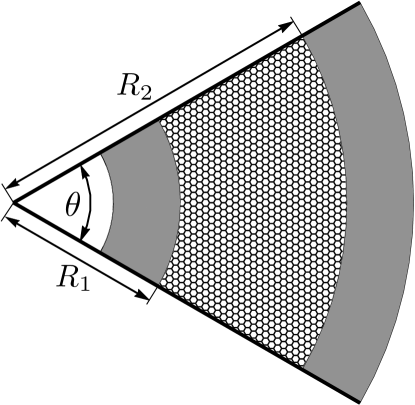
Figure 1: A section of the Corbino disk in graphene attached to two metal contacts (shaded areas). Tick lines at the system edges depict infinite-mass boundary conditions. The opening angle $\theta=\pi/3$ and the radii ratio $R_{2}/R_{1}=2$ are set for an illustration only.

II Model

Our system is a section of the Corbino disk in graphene characterized by the opening angle $\theta$ and the inner (outer) radius $R_{1}$ ($R_{2}$) (see Fig.1). The leads are modelled with heavily-doped graphene areas key-6 . Mode-matching analysis (see Appendices A and B) gives the transmission amplitudes for quasiparticles passing through the sample area. The conductance is obtained by summing the transmission probabilities over the modes in the Landauer-Büttiker formula

$$G=G_{0}\sum_{j}\left|t_{j}\right|^{2},$$ (1)

with $G_{0}=4e^{2}/h$ due to spin and valley degeneracies.

As the wavefunctions should in general posses cylindrical symmetry, we start from the analysis of the full disk. The Dirac equation in polar coordinates $(r,\phi)$ can be written as

$$\left[\begin{array}[]{cc}\epsilon&e^{-i\phi}\left(i\partial_{r}\!+\!\cfrac{\partial_{\phi}}{r}\right)\\ e^{i\phi}\left(i\partial_{r}\!-\!\cfrac{\partial_{\phi}}{r}\right)&\epsilon\end{array}\right]\left(\begin{array}[]{c}\psi_{A}\\ \psi_{B}\end{array}\right)=0,$$ (2)

where $\epsilon=\left(E-V\right)/\hbar v_{F}$, $v_{F}\approx c/300$ is the Fermi velocity, and the electrostatic potential energy is

$$V(r)=\begin{cases}-V_{\infty}&\mbox{if $r<R_{1}\mbox{ or }r>R_{2}$,}\\ 0&\mbox{if $R_{1}<r<R_{2}$}.\end{cases}$$ (3)

Since the Hamiltonian commutes with the total angular momentum operator $J_{z}=-i\hbar\partial_{\phi}+\hbar\sigma_{z}/2$, the wavefunction

$$\psi_{j}\left(r,\phi\right)=\exp\left[i\phi\left(j-1/2\right)\right]\left(\begin{array}[]{c}\varphi_{A}\left(r\right)\\ \exp\left(i\phi\right)\varphi_{B}\left(r\right)\end{array}\right),$$ (4)

where $j=\pm\frac{1}{2},\pm\frac{3}{2},\dots$ is the angular momentum quantum number. Substituting $\psi_{j}$ into Eq. (2) we can derive

$$\varphi_{j}\left(r\right)\equiv\left(\begin{array}[]{c}\varphi_{A}\left(r\right)\\ \varphi_{B}\left(r\right)\end{array}\right)=\left(\begin{array}[]{c}\mbox{H}_{j-1/2}^{\left(\zeta\right)}\left(\epsilon r\right)\\ i\mbox{H}_{j+1/2}^{\left(\zeta\right)}\left(\epsilon r\right)\end{array}\right),$$ (5)

where $H_{\nu}^{(\zeta)}$, with $\zeta=2(1)$ for the incoming (outgoing) waves, is the Hankel function of the second (first) kind key-11 . The momentum-independent radial current density is $\left({\bf j}\right)_{r}=-ev_{F}\,\psi_{j}^{\dagger}\left(\sigma_{x}\cos\phi+\sigma_{y}\sin\phi\right)\psi_{j}=4\lambda_{\zeta}ev_{F}/(\pi\epsilon{}r)$, with $\lambda_{\zeta}=(-1)^{\zeta}$. In the high-doping limit $\varphi_{j}\left(r\right)$ (5) simplifies to

$$\varphi_{j}\left(r\right)\overset{\left|\epsilon\right|\rightarrow\infty}{\simeq}\sqrt{\frac{2}{\pi\epsilon r}}\exp\left[-i\lambda_{\zeta}\left(\epsilon r-\pi{}j/2\right)\right]\left(\begin{array}[]{c}1\\ -\lambda_{\zeta}\end{array}\right).$$ (6)

Now, the sample edges are introduced to our analysis via the infinite-mass boundary conditions. Following Ref. key-10 , we demand that the angular current vanishes at the sample edges; i.e., $\left({\bf j}\right)_{n}=\hat{\bf n}\cdot\left[\psi_{j}^{\dagger}\left(\hat{x}\sigma_{x}+\hat{y}\sigma_{y}\right)\psi_{j}\right]=0$, where $\hat{\bf n}$ denotes the unit vector normal to the boundary. This leads to

$$\psi_{B}/\psi_{A}=i\exp(\gamma),$$ (7)

where $\gamma=0$ for $\phi=\pi/2$ or $\gamma=\theta+\pi$ for $\phi=\theta+\pi/2$ (without loss of generality we set the boarders at $\phi=\pi/2$ and $\phi=\theta+\pi/2$). In particular, for $\theta=\pi/(2k+1)$ with $k=0,1,2,\dots$, the solutions can be found as linear combinations of the form $a_{j}\psi_{j}+b_{j}\psi_{-j}$ and are given explicitly in Appendix A. Due to Eq. (7), the values of $j$ contributing to the sum in Eq. (1) are further restricted to

$$j=-\frac{\pi\left(2n-1\right)}{2\theta},\ \ \ \ n=1,2,3,\dots.$$ (8)

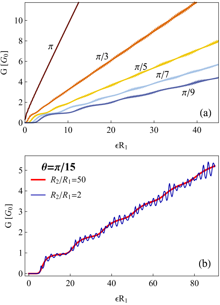
Figure 2: (a) Conductance of the disk section as a function of doping for the opening angle varying from $\theta=\pi$ down to $\pi/9$ (specified for each curve) and the radii ratio fixed at $R_{2}/R_{1}=10$. (b) Same as (a) but for $\theta=\pi/15$ and two values of $R_{2}/R_{1}$. Notice the suppression of the Fabry-Perot oscillations for $R_{2}/R_{1}=50$.

III Conductance quantization

The numerical results for disk sections with different geometric parameters are presented in Fig. 2. For small radii ratios $R_{2}/R_{1}\lesssim{}2$ and large opening angles $\theta\gtrsim\pi/3$, the approximating formula for the pseudodiffusive limit key-9

$$G_{{\rm diff}}\approx\frac{4e^{2}}{\pi h}\,\frac{\theta}{\ln(R_{2}/R_{1})}$$ (9)

reproduces the exact values obtained via Eq. (1) for $\epsilon\rightarrow{}0$. In other cases, the conductance near the Dirac point is highly suppressed due to the limited number of transmission modes. At higher dopings and for $R_{2}/R_{1}\lesssim{}10$, we notice the Fabry-Perot oscillations arising from strong interference between the incoming and outgoing waves in the sample area. The conductance quantization is clearly visible for $\theta\lesssim\pi/3$. Decreasing $\theta$, one can systematically increase the number of sharp conductance steps (see Fig. 2a).

To describe the above-mentioned effect in a quantitative manner, we plotted (in Fig. 3) the squared step width $\Delta\mu^{2}$ of several consecutive conductance steps ($1\leqslant{}n\leqslant{}7$) for $R_{2}/R_{1}=10$ and different angles $\theta$. The $n$-th step width is quantified by the inverse slope of the straight line least-square fitted to the exact conductance-doping dependence; i.e.,

$$G/G_{0}\approx\frac{1}{\sqrt{\Delta\mu^{2}}}\,\epsilon{}R_{1}+{\rm const},$$ (10)

where the fitting is performed near the inflection point corresponding to the $n$-th conductance step. Remarkably, $\Delta\mu^{2}$ increases systematically with $n$. This observation can be rationalized by calculating the transmission probability for electrostatic potential barrier within the semiclassical approximation key-13 . For the classically forbidden regime, $R_{1}<r<j/\epsilon$, one can write

$$T_{j}\approx\exp\left[\,-2\intop_{R_{1}}^{j/\epsilon}\!dr\,\sqrt{\left(\frac{j}{r}\right)^{2}-\epsilon^{2}}\ \right],$$ (11)

where $j/r$ [with $j$ given by Eq. (8)] plays a role of the transverse wavenumber, and we have further supposed that $R_{2}\gg{}R_{1}$. Each individual step, associated with the inflection point on the conductance-doping plot, corresponds to $T_{j}\approx{}1/2$ for a given $j$. A clear step becomes visible when $T_{j}$ rises fast enough with $\epsilon$, such that the step width is significantly smaller than distances to the neighboring steps. These lead to

$$\sqrt{n}\,\theta/\pi\ll{}1.$$ (12)

In turn, for any finite $\theta$ only a limited number of the conductance steps near zero doping ($n\leqslant{}n_{\rm max}$) is visible, whereas the higher steps get smeared out. This effect has no direct analogue in similar Schrödinger systems.

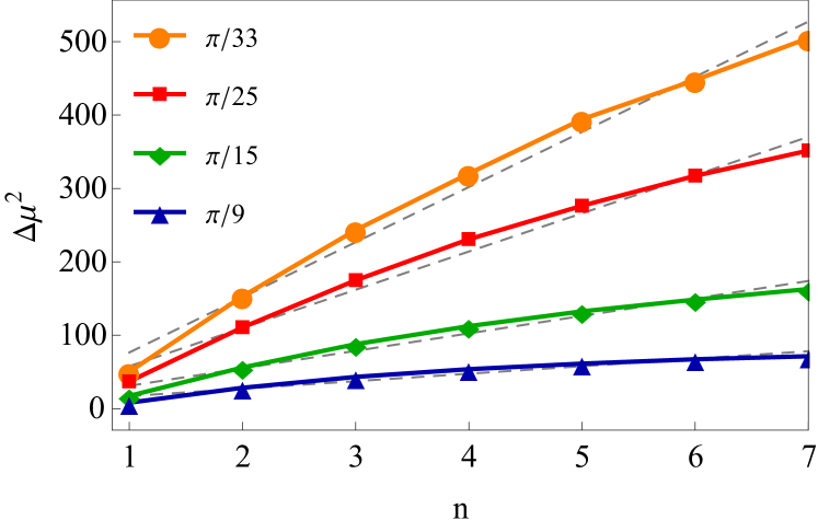
Figure 3: Squared width $\Delta\mu^{2}$ versus the step index $n$ for $R_{2}/R_{1}=10$ and different values of $\theta$. Solid lines are guides for the eye only; dashed lines depict best-fitted linear dependence of $\Delta\mu^{2}$ on $n$.

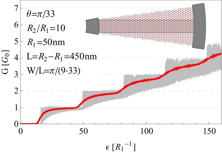
Figure 4: Conductance as a function of doping for graphene nanoribbon (thin gray line) and narrow disk section (thick red line). Inset: Schematics of the two systems considered.

We compare now our results with more familiar conductance quantization appearing for GNRs, using the analytic formula for a strip with infinite-mass boundary conditions derived by Tworzydło et al. key-6 . In fact, a rectangular sample of the width $W=\theta R_{1}$ and the length $L=R_{2}-R_{1}$ essentially reproduces a geometric quantization appearing in a disk section for small opening angles. As shown in Fig. 4, the conductance-doping curves for the two systems closely follow each other, except from the Fabry-Perot oscillations present in GNR and strongly suppressed in the disk section with nonparallel borders.

IV Conclusion

We have investigated ballistic charge transport through a finite section of the Corbino disk in graphene with the infinite-mass boundaries. The system conductance as a function of doping shows sharp quantization steps for opening angles $\theta\lesssim\pi/3$. In comparison to the situation in graphene nanoribbons, Fabry-Perot oscillations are strongly suppressed, particularly for large radii ratios $R_{2}/R_{1}\gtrsim{}10$. For these reasons, our theoretical study suggests that a narrow section of the disk, or a triangle, may be the most suitable sample geometry for experimental demonstration of the conductance quantization in graphene or other Dirac system.

Additionally, a special feature of the conductance-doping dependence for Dirac systems has been identified. Namely, the quantization steps are blurred such that the step width is proportional to $\sqrt{n}$, with $n$ being the step number. This observation helps to understand why only a very limited number of sharp conductance steps were identified so far in both experimental key-8 and numerical studies key-7 .

Appendix A: Wavefunctions

In this Appendix we give explicitly the pairs of linearly-independent solutions $\left[f_{A,j},f_{B,j}\right]^{T}$ and $\left[g_{A,j},g_{B,j}\right]^{T}$ of Eq. (2) with the boundary conditions (7). For the leads ($r<R_{1}$ or $r>R_{2}$) we define the dimensionless variable $\rho=\epsilon_{\infty}{}r$ and get

$$f_{\alpha,j}^{L}(\rho,\phi) = \sqrt{\frac{8}{\pi\rho}}\exp\left[i\left(\rho\mp\phi/2\right)\right]\cos\left[j\left(\phi-\frac{\pi}{2}\right)\right],$$ (13)

$$g_{\alpha,j}^{L}(\rho,\phi) = \pm\sqrt{\frac{8}{\pi\rho}}\exp\left[-i\left(\rho\pm\phi/2\right)\right]\cos\left[j\left(\phi+\frac{\pi}{2}\right)\right],$$ (14)

where the upper (lower) signs correspond to the sublattice index $\alpha=A$ ($\alpha=B$). Similarly, for the sample area ($R_{1}<r<R_{2}$) $\rho=\epsilon{}r$, and the wavefunctions read

$$f_{A,j}^{S}(\rho,\phi) = \exp\left[i(j+1/2)(\pi-\phi)\right]\mbox{H}_{j+1/2}^{(1)}(\rho)+\exp\left[i\left(j-1/2\right)\phi\right]\mbox{H}_{j-1/2}^{(1)}(\rho),$$ (15)

$$f_{B,j}^{S}(\rho,\phi) = i\left\{\exp\left[i\left(j+1/2\right)\phi\right]\mbox{H}_{j+1/2}^{(1)}(\rho)+\exp\left[i(j-1/2)(\pi-\phi)\right]\mbox{H}_{j-1/2}^{(1)}(\rho)\right\},$$ (16)

$$g_{A,j}^{S}(\rho,\phi) = \exp\left[-i(j+1/2)(\phi+\pi)\right]\mbox{H}_{j+1/2}^{(2)}(\rho)+\exp\left[i\left(j-1/2\right)\phi\right]\mbox{H}_{j-1/2}^{(2)}(\rho),$$ (17)

$$g_{B,j}^{S}(\rho,\phi) = i\left\{\exp\left[i\left(j+1/2\right)\phi\right]\mbox{H}_{j+1/2}^{(2)}(\rho)+\exp\left[-i(j-1/2)(\phi+\pi)\right]\mbox{H}_{j-1/2}^{(2)}(\rho)\right\}.$$ (18)

Appendix B: Mode-matching

The current conservation conditions at $r=R_{1}$ and $r=R_{2}$ lead to the system of linear equations

$$\left(\begin{array}[]{cccc}0&-f_{A,j}^{L}(\epsilon_{\infty}R_{1},\phi)&f_{A,j}^{S}(\epsilon R_{1},\phi)&g_{A,j}^{S}(\epsilon R_{1},\phi)\\ 0&-f_{B,j}^{L}(\epsilon_{\infty}R_{1},\phi)&f_{B,j}^{S}(\epsilon R_{1},\phi)&g_{B,j}^{S}(\epsilon R_{1},\phi)\\ -g_{A,j}^{L}(\epsilon_{\infty}R_{2},\phi)&0&f_{A,j}^{S}(\epsilon R_{2},\phi)&g_{A,j}^{S}(\epsilon R_{2},\phi)\\ -g_{B,j}^{L}(\epsilon_{\infty}R_{2},\phi)&0&f_{B,j}^{S}(\epsilon R_{2},\phi)&g_{B,j}^{S}(\epsilon R_{2},\phi)\end{array}\right)\left(\begin{array}[]{c}t_{j}\\ r_{j}\\ a_{j}\\ b_{j}\end{array}\right)=\left(\begin{array}[]{c}g_{A,j}^{L}(\epsilon_{\infty}R_{1},\phi)\\ g_{B,j}^{L}(\epsilon_{\infty}R_{1},\phi)\\ 0\\ 0\end{array}\right),$$ (19)

where we have supposed that the wave is incident from the inner lead. We further notice that the transmission probability $|t_{j}|^{2}$ is insensitive to the specific value of $\epsilon_{\infty}$, as it only affects the phases of wavefunctions $f_{\alpha,j}^{L}$ (13) and $g_{\alpha,j}^{L}$ (14).

References

- (1) B.J. van Wees, H. van Houten, C.W.J. Beenakker, J.G. Williamson, L.P. Kouwenhoven, D. van der Marel, and C.T. Foxon, Phys. Rev. Lett. 60, 848 (1988); D.A. Wharam, T.J. Thornton, R. Newbury, M. Pepper, H. Ahmed, J.E.F. Frost, D.G. Hasko, D.C. Peacock, D.A. Ritchie, and G.A.C. Jones, J. Phys. C: Solid State Phys. 21, L209 (1988).
- (2) L.I. Glazman, G.B. Lesovik, D.E. Khmel’nitskii, and R.I. Shekhter, Pis’ma Zh. Eksp. Teor. Fiz. 48 No. 4, 218 (1988).
- (3) Yu.V. Nazarov and Ya.M. Blanter, Quantum Transport: Introduction to Nanoscience, Cambridge University Press (Cambridge 2009), Chapter 1.
- (4) G. Kirczenow, J. Phys.: Condens. Matter 6, L583 (1994); S. Souma and A. Suzuki, Phys. Rev. B 58, 4649 (1998).
- (5) J. Tworzydło, B. Trauzettel, M. Titov, A. Rycerz, and C.W.J. Beenakker, Phys. Rev. Lett. 96, 246802 (2006).
- (6) A. Rycerz, J. Tworzydło and C.W.J. Beenakker, Nature Phys. 3, 172 (2007); A. Rycerz, phys. stat. sol. (a) 205, 1281 (2008).
- (7) J. Wurm, M. Wimmer, I. Adagideli, K. Richter, and H.U. Baranger, New J. Phys. 11, 095022 (2009); A. Rycerz, Acta Phys. Polon. A 118, 238 (2010).
- (8) S. Ihnatsenka and G. Kirczenow, Phys. Rev. B 85, 121407 (2012).
- (9) N. Tombros, A. Veligura, J. Junesch, M.H.D. Guimaraes, I.J. Vera-Marun, H.T. Jonkman, and B.J. van Wees, Nature Phys. 7, 697 (2011); B. Özyilmaz, P. Jarillo-Herrero, D. Efetov, and P. Kim, Appl. Phys. Lett. 91, 192107 (2007).
- (10) A. Rycerz, P. Recher, and M. Wimmer, Phys. Rev. B 80, 125417 (2009).
- (11) A. Rycerz, Phys. Rev. B 81, 121404(R) (2010); M.I. Katsnelson, Europhys. Lett. 89, 17001 (2010).
- (12) Z. Khatibi, H. Rostami, and R. Asgari, Phys. Rev. B 88, 195426 (2013).
- (13) M.V. Berry and R.I. Mondragon, Proc. R. Soc. A 41, 53 (1987).
- (14) A.R. Akhmerov and C.W.J. Beenakker, Phys. Rev. B 77, 085423 (2008); C.G. Beneventano and E.M. Santangelo, Int. J. Mod. Phys. Conf. Ser. 14, 240 (2012).
- (15) M. Abramowitz and I.A. Stegun, eds., Handbook of Mathematical Functions (Dover Publications, Inc., New York, 1965), Chapter 9.
- (16) V.V. Cheianov and V.I. Fal’ko, Phys. Rev. B 74, 041403(R) (2006); K.J.A. Reijnders, T. Tudorovskiy, and M.I. Katsnelson, Ann. of Phys. 333, 155 (2013).