On the Learning Behavior of Adaptive Networks — Part I: Transient Analysis

Abstract

This work carries out a detailed transient analysis of the learning behavior of multi-agent networks, and reveals interesting results about the learning abilities of distributed strategies. Among other results, the analysis reveals how combination policies influence the learning process of networked agents, and how these policies can steer the convergence point towards any of many possible Pareto optimal solutions. The results also establish that the learning process of an adaptive network undergoes three (rather than two) well-defined stages of evolution with distinctive convergence rates during the first two stages, while attaining a finite mean-square-error (MSE) level in the last stage. The analysis reveals what aspects of the network topology influence performance directly and suggests design procedures that can optimize performance by adjusting the relevant topology parameters. Interestingly, it is further shown that, in the adaptation regime, each agent in a sparsely connected network is able to achieve the same performance level as that of a centralized stochastic-gradient strategy even for left-stochastic combination strategies. These results lead to a deeper understanding and useful insights on the convergence behavior of coupled distributed learners. The results also lead to effective design mechanisms to help diffuse information more thoroughly over networks.

I INTRODUCTION

In multi-agent systems, agents interact with each other to solve a problem of common interest, such as an optimization problem in a distributed manner. Such networks of interacting agents are useful in solving distributed estimation, learning and decision making problems [2, 3, 4, 5, 6, 7, 8, 9, 10, 11, 12, 13, 14, 15, 16, 17, 18, 19, 20, 21, 22, 23, 24, 25, 26, 27, 28, 29, 30, 31, 32, 33, 34, 35, 36, 37, 38, 39]. They are also useful in modeling biological networks[40, 41, 42], collective rational behavior[12, 13], and in developing biologically-inspired designs[2, 43]. Two useful strategies that can be used to guide the interactions of agents over a network are consensus strategies [10, 11, 5, 6, 7, 8, 9] and diffusion strategies[16, 17, 18, 19, 20, 21, 22, 23, 24, 25, 26, 27]. Both classes of algorithms involve self-learning and social-learning steps. During self-learning, each agent updates its state using its local data. During social learning, each agent aggregates information from its neighbors. A useful feature that results from these localized interactions is that the network ends up exhibiting global patterns of behavior. For example, in distributed estimation and learning, each agent is able to attain the performance of centralized solutions by relying solely on local cooperation [6, 19, 22, 23].

In this article, and the accompanying Part II [44], we consider a general class of distributed strategies, which includes diffusion and consensus updates as special cases, and study the resulting global learning behavior by addressing four important questions: (i) where does the distributed algorithm converge to? (ii) when does it converge? (iii) how fast does it converge? and (iv) how close does it converge to the intended point? We answer questions (i)–(iii) in Part I and question (iv) in Part II [44]. We study these four questions by characterizing the learning dynamics of the network in some great detail. An interesting conclusion that follows from our analysis is that the learning curve of a multi-agent system will be shown to exhibit three different phases. In the first phase (Transient Phase I), the convergence rate of the network is determined by the second largest eigenvalue of the combination matrix in magnitude, which is related to the degree of network connectivity. In the second phase (Transient Phase II), the convergence rate is determined by the entries of the right-eigenvector of the combination matrix corresponding to the eigenvalue at one. And, in the third phase (the steady-state phase) the mean-square performance of the algorithm turns out to depend on this same right-eigenvector in a revealing way. Even more surprisingly, we shall discover that the agents have the same learning behavior starting at Transient Phase II, and are able to achieve a performance level that matches that of a fully connected network or a centralized stochastic-gradient strategy. Actually, we shall show that the consensus and diffusion strategies can be represented as perturbed versions of a centralized reference recursion in a certain transform domain. We quantify the effect of the perturbations and establish the aforementioned properties for the various phases of the learning behavior of the networks. The results will reveal the manner by which the network topology influences performance in some unexpected ways.

There have been of course many insightful works in the literature on distributed strategies and their convergence behavior. In Sections II-B and IV-A further ahead, we explain in what ways the current manuscript extends these earlier investigations and what novel contributions this work leads to. In particular, it will be seen that several new insights are discovered that clarify how distributed networks learn. For the time being, in these introductory remarks, we limit ourselves to mentioning one important aspect of our development. Most prior studies on distributed optimization and estimation tend to focus on the performance and convergence of the algorithms under diminishing step-size conditions[5, 6, 7, 8, 9, 28, 29, 10, 30, 45], or on convergence under deterministic conditions on the data[10]. This is perfectly fine for applications involving static optimization problems where the objective is to locate the fixed optimizer of some aggregate cost function of interest. In this paper, however, we examine the learning behavior of distributed strategies under constant step-size conditions. This is because constant step-sizes are necessary to enable continuous adaptation, learning, and tracking in the presence of streaming data and drifting conditions. These features would enable the algorithms to perform well even when the location of the optimizer drifts with time. Nevertheless, the use of constant step-sizes enriches the dynamics of (stochastic-gradient) distributed algorithms in that the gradient update term does not die out with time anymore, in clear contrast to the diminishing step-size case where the influence of the gradient term is annihilated over time due to the decaying value of the step-size parameter. For this reason, more care is needed to examine the learning behavior of distributed strategies in the constant step-size regime since their updates remain continually active and the effect of gradient noise is always present. This work also generalizes and extends in non-trivial ways the studies in [18, 20]. For example, while reference [18] assumed that the individual costs of all agents have the same minimizer, and reference [20] assumed that each of these individual costs is strongly convex, these requirements are not needed in the current study: individual costs can have distinct minimizers and they do not even need to be convex (see the discussion after expression (32)). This fact widens significantly the class of distributed learning problems that are covered by our framework. Moreover, the network behavior is studied under less restrictive assumptions and for broader scenarios, including a close study of the various phases of evolution during the transient phase of the learning process. We also study a larger class of distributed strategies that includes diffusion and consensus strategies as special cases.

To examine the learning behavior of adaptive networks under broader and more relaxed conditions than usual, we pursue a new analysis route by introducing a reference centralized recursion and by studying the perturbation of the diffusion and consensus strategies relative to this centralized solution over time. Insightful new results are obtained through this perturbation analysis. For example, we are now able to examine closely both the transient phase behavior and the steady-state phase behavior of the learning process and to explain how behavior in these two stages relate to the behavior of the centralized solution (see Fig. 2 further ahead). Among several other results, the mean-square-error expression (52) derived later in Part II [44] following some careful analysis, which builds on the results of this Part I, is one of the new (compact and powerful) insights; it reveals how the performance of each agent is closely related to that of the centralized stochastic approximation strategy — see the discussion right after (52). As the reader will ascertain from the derivations in the appendices, arriving at these conclusions for a broad class of distributed strategies and under weaker conditions than usual is demanding and necessitates a careful study of the evolution of the error dynamics over the network and its stability. When all is said and done, Parts I and II [44] lead to several novel insights into the learning behavior of adaptive networks.

Notation. All vectors are column vectors. We use boldface letters to denote random quantities (such as $\bm{u}_{k,i}$) and regular font to denote their realizations or deterministic variables (such as $u_{k,i}$). We use $\mathrm{diag}\{x_{1},\ldots,x_{N}\}$ to denote a (block) diagonal matrix consisting of diagonal entries (blocks) $x_{1},\ldots,x_{N}$, and use $\mathrm{col}\{x_{1},\ldots,x_{N}\}$ to denote a column vector formed by stacking $x_{1},\ldots,x_{N}$ on top of each other. The notation $x\preceq y$ means each entry of the vector $x$ is less than or equal to the corresponding entry of the vector $y$, and the notation $X\preceq Y$ means each entry of the matrix $X$ is less than or equal to the corresponding entry of the matrix $Y$. The notation $x=\mathrm{vec}(X)$ denotes the vectorization operation that stacks the columns of a matrix $X$ on top of each other to form a vector $x$, and $X=\mathrm{vec}^{-1}(x)$ is the inverse operation. The operators $\nabla_{w}$ and $\nabla_{w^{T}}$ denote the column and row gradient vectors with respect to $w$. When $\nabla_{w^{T}}$ is applied to a column vector $s$, it generates a matrix. The notation $a(\mu)=O(b(\mu))$ means that there exists a constant $C>0$ such that for all $\mu$, $a(\mu)\leq C\cdot b(\mu)$.

II PROBLEM FORMULATION

II-A Distributed Strategies: Consensus and Diffusion

We consider a connected network of $N$ agents that are linked together through a topology — see Fig. 1. Each agent $k$ implements a distributed algorithm of the following form to update its state vector from $\bm{w}_{k,i-1}$ to $\bm{w}_{k,i}$:

$$\bm{\phi}_{k,i-1} =\sum_{l=1}^{N}a_{1,lk}\bm{w}_{l,i-1}$$ (1)

$$\bm{\psi}_{k,i} =\sum_{l=1}^{N}a_{0,lk}\bm{\phi}_{l,i-1}-\mu_{k}\hat{\bm{s}}_{k,i}(\bm{\phi}_{k,i-1})$$ (2)

$$\bm{w}_{k,i} =\sum_{l=1}^{N}a_{2,lk}\bm{\psi}_{l,i}$$ (3)

where $\bm{w}_{k,i}\in\mathbb{R}^{M}$ is the state of agent $k$ at time $i$, usually an estimate for the solution of some optimization problem, $\bm{\phi}_{k,i-1}\in\mathbb{R}^{M}$ and $\bm{\psi}_{k,i}\in\mathbb{R}^{M}$ are intermediate variables generated at node $k$ before updating to $\bm{w}_{k,i}$, $\mu_{k}$ is a non-negative constant step-size parameter used by node $k$, and $\hat{\bm{s}}_{k,i}(\cdot)$ is an $M\times 1$ update vector function at node $k$. In deterministic optimization problems, the update vectors $\hat{\bm{s}}_{k,i}(\cdot)$ can be the gradient or Newton steps associated with the cost functions[10]. On the other hand, in stocastic approximation problems, such as adaptation, learning and estimation problems [5, 6, 8, 7, 9, 14, 26, 15, 16, 17, 19, 18, 20, 23, 22, 25, 28, 29, 21, 27], the update vectors are usually computed from realizations of data samples that arrive sequentially at the nodes. In the stochastic setting, the quantities appearing in (1)–(3) become random and we use boldface letters to highlight their stochastic nature. In Example 1 below, we illustrate choices for $\hat{\bm{s}}_{k,i}(w)$ in different contexts.

The combination coefficients $a_{1,lk}$, $a_{0,lk}$ and $a_{2,lk}$ in (1)–(3) are nonnegative weights that each node $k$ assigns to the information arriving from node $l$; these coefficients are required to satisfy:

$$\sum_{l=1}^{N}a_{1,lk}=1,\quad\sum_{l=1}^{N}a_{0,lk}=1,\quad\sum_{l=1}^{N}a_{2,lk}=1$$ (4)

$$a_{1,lk}\geq 0,\qquad a_{0,lk}\geq 0,\qquad a_{2,lk}\geq 0$$ (5)

$$a_{1,lk}=a_{2,lk}=a_{0,lk}=0,\qquad\mathrm{if~{}}l\notin\mathcal{N}_{k}$$ (6)

Observe from (6) that the combination coefficients are zero if $l\notin\mathcal{N}_{k}$, where $\mathcal{N}_{k}$ denotes the set of neighbors of node $k$. Therefore, each summation in (1)–(3) is actually confined to the neighborhood of node $k$. In algorithm (1)–(3), each node $k$ first combines the states $\{\bm{w}_{l,i-1}\}$ from its neighbors and updates $\bm{w}_{k,i-1}$ to the intermediate variable $\bm{\phi}_{k,i-1}$. Then, the $\{\bm{\phi}_{l,i-1}\}$ from the neighbors are aggregated and updated to $\bm{\psi}_{k,i}$ along the opposite direction of $\hat{\bm{s}}_{k,i}(\bm{\phi}_{k,i-1})$. Finally, the intermediate estimators $\{\bm{\psi}_{l,i}\}$ from the neighbors are combined to generate the new state $\bm{w}_{k,i}$ at node $k$.

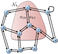
Figure 1: A network representing a multi-agent system. The set of all agents that can communicate with node $k$ is denoted by $\mathcal{N}_{k}$.The edge linking any two agents is represented by two directed arrows to emphasize that information can flow in both directions.

Example 1

The distributed algorithm (1)–(3) can be applied to optimize aggregate costs of the following form:

$$J^{\mathrm{glob}}(w)=\sum_{k=1}^{N}J_{k}(w)$$ (7)

or to find Pareto-optimal solutions to multi-objective optimization problems, such as:

$$\min_{w}\left\{J_{1}(w),\ldots,J_{N}(w)\right\}$$ (8)

where $J_{k}(w)$ is an individual convex cost associated with each agent $k$. Optimization problems of the form (7)–(8) arise in various applications — see [3, 4, 5, 6, 7, 8, 9, 10, 11, 12, 13, 14, 15, 26, 21, 16, 17, 19, 18, 20, 27, 23, 22, 24, 25, 28, 29, 30, 31]. Depending on the context, the update vector $\hat{\bm{s}}_{k,i}(\cdot)$ may be chosen in different ways:

• In deterministic optimization problems, the expressions for $\{J_{k}(w)\}$ are known and the update vector $\hat{\bm{s}}_{k,i}(\cdot)$ at node $k$ is chosen as the deterministic gradient (column) vector $\nabla_{w}J_{k}(\cdot)$.

• In distributed estimation and learning, the individual cost function at each node $k$ is usually selected as the expected value of some loss function $Q_{k}(\cdot,\cdot)$, i.e., $J_{k}(w)=\mathbb{E}\{Q_{k}(w,\bm{x}_{k,i})\}$ [18], where the expectation is with respect to the randomness in the data samples $\{\bm{x}_{k,i}\}$ collected at node $k$ at time $i$. The exact expression for $\nabla_{w}J_{k}(w)$ is usually unknown since the probability distribution of the data is not known beforehand. In these situations, the update vector $\hat{\bm{s}}_{k,i}(\cdot)$ is chosen as an instantaneous approximation for the true gradient vector, such as, $\hat{\bm{s}}_{k,i}(\cdot)=\widehat{\nabla_{w}J_{k}}(\cdot)=\nabla_{w}Q_{k}(\cdot,\bm{x}_{k,i})$, which is known as stochastic gradient. Note that the update vector $\hat{\bm{s}}_{k,i}(w)$ is now evaluated from the random data sample $\bm{x}_{k,i}$. Therefore, it is also random and time dependent.

The update vectors $\{\hat{\bm{s}}_{k,i}(\cdot)\}$ may not necessarily be the gradients of cost functions or their stochastic approximations. They may take other forms for different reasons. For example, in [6], a certain gain matrix $K$ is multiplied to the left of the stochastic gradient vector $\widehat{\nabla_{w}J_{k}}(\cdot)$ to make the estimator asymptotically efficient for a linear observation model. ∎

Returning to the general distributed strategy (1)–(3), we note that it can be specialized into various useful algorithms. We let $A_{1}$, $A_{0}$ and $A_{2}$ denote the $N\times N$ matrices that collect the coefficients $\{a_{1,lk}\}$, $\{a_{0,lk}\}$ and $\{a_{2,lk}\}$. Then, condition (4) is equivalent to

$$A_{1}^{T}\mathds{1}=\mathds{1},\quad A_{0}^{T}\mathds{1}=\mathds{1},\quad A_{2}^{T}\mathds{1}=\mathds{1}$$ (9)

where $\mathds{1}$ is the $N\times 1$ vector with all its entries equal to one. Condition (9) means that the matrices $\{A_{0},A_{1},A_{2}\}$ are left-stochastic (i.e., the entries on each of their columns add up to one). Different choices for $A_{1}$, $A_{0}$ and $A_{2}$ correspond to different distributed strategies, as summarized in Table I. Specifically, the traditional consensus[10, 11, 5, 6, 7, 8, 9] and diffusion (ATC and CTA) [16, 21, 17, 19, 18, 20, 23, 22] algorithms with constant step-sizes are given by the following iterations:

$$\mathrm{Consensus:}\; \begin{cases}\displaystyle\bm{\phi}_{k,i-1}=\sum_{l\in\mathcal{N}_{k}}\!\!a_{0,lk}\bm{w}_{l,i-1}\\ \displaystyle\bm{w}_{k,i}=\bm{\phi}_{k,i-1}-\mu_{k}\hat{\bm{s}}_{k,i}(\bm{w}_{k,i-\!1})\end{cases}$$ (10)

$$\mathrm{CTA~{}diffusion:}\; \begin{cases}\displaystyle\bm{\phi}_{k,i-1}=\sum_{l\in\mathcal{N}_{k}}a_{1,lk}\bm{w}_{l,i-1}\\ \bm{w}_{k,i}=\bm{\phi}_{k,i-1}-\mu_{k}\hat{\bm{s}}_{k,i}(\bm{\phi}_{k,i-1})\end{cases}$$ (11)

$$\mathrm{ATC~{}diffusion:}\; \begin{cases}\displaystyle\bm{\psi}_{k,i}=\bm{w}_{k,i-1}\!-\!\mu_{k}\hat{\bm{s}}_{k,i}(\bm{w}_{k,i-1})\\ \displaystyle\bm{w}_{k,i}=\sum_{l\in\mathcal{N}_{k}}a_{2,lk}\bm{\psi}_{l,i}\end{cases}$$ (12)

Therefore, the convex combination steps appear in different locations in the consensus and diffusion implementations. For instance, observe that the consensus strategy (10) evaluates the update direction $\hat{\bm{s}}_{k,i}(\cdot)$ at $\bm{w}_{k,i-1}$, which is the estimator prior to the aggregation, while the diffusion strategy (11) evaluates the update direction at $\bm{\phi}_{k,i-1}$, which is the estimator after the aggregation. In our analysis, we will proceed with the general form (1)–(3) to study all three schemes, and other possibilities, within a unifying framework.

TABLE I: Different choices for $A_{1}$, $A_{0}$ and $A_{2}$ correspond to different distributed strategies.

Distributed Strategeis	$A_{1}$	$A_{0}$	$A_{2}$	$A_{1}A_{0}A_{2}$
Consensus	$I$	$A$	$I$	$A$
ATC diffusion	$I$	$I$	$A$	$A$
CTA diffusion	$A$	$I$	$I$	$A$

We observe that there are two types of learning processes involved in the dynamics of each agent $k$: (i) self-learning in (2) from locally sensed data and (ii) social learning in (1) and (3) from neighbors. All nodes implement the same self- and social learning structure. As a result, the learning dynamics of all nodes in the network are coupled; knowledge exploited from local data at node $k$ will be propagated to its neighbors and from there to their neighbors in a diffusive learning process. It is expected that some global performance pattern will emerge from these localized interactions in the multi-agent system. In this work and the accompanying Part II [44], we address the following questions:

• Limit point: where does each state $\bm{w}_{k,i}$ converge to?

• Stability: under which condition does convergence occur?

• Learning rate: how fast does convergence occur?

• Performance: how close is $\bm{w}_{k,i}$ to the limit point?

• Generalization: can $\bm{w}_{k,i}$ match the performance of a centralized solution?

We address the first three questions in this part, and examine the last two questions pertaining to performance in Part II [44]. We address the five questions by characterizing analytically the learning dynamics of the network to reveal the global behavior that emerges in the small step-size regime. The answers to these questions will provide useful and novel insights about how to tune the algorithm parameters in order to reach desired performance levels — see Sec. LABEL:P2-Sec:Benefits in Part II [44].

II-B Relation to Prior Work

In comparison with the existing literature[5, 6, 7, 8, 9, 28, 29, 10, 30, 45, 46, 47, 48], it is worth noting that most prior studies on distributed optimization algorithms focus on studying their performance and convergence under diminishing step-size conditions and for doubly-stochastic combination policies (i.e., matrices for which the entries on each of their columns and on each of their rows add up to one). These are of course useful conditions, especially when the emphasis is on solving static optimization problems. We focus instead on the case of constant step-sizes because, as explained earlier, they enable continuous adaptation and learning under drifting conditions; in contrast, diminishing step-sizes turn off learning once they approach zero. By using constant step-sizes, the resulting algorithms are able to track dynamic solutions that may slowly drift as the underlying problem conditions change.

Moreover, constant step-size implementations have merits even for stationary environments where the solutions remain static. This is because, as we are going to show later in this work and its accompanying Part II [44], constant step-size learning converges at a geometric rate, in the order of $O(\gamma^{i})$ for some $0<\gamma<1$, towards a small mean-square error in the order of the step-size parameter. This means that these solutions can attain satisfactory performance even after short intervals of time. In comparison, implementations that rely on a diminishing step-size of the form $\mu(i)=\mu_{o}/i$, for some constant $\mu_{o}$, converge almost surely to the solution albeit at the slower rate of $O(1/i)$. Furthermore, the choice of the parameter $\mu_{o}$ is critical to guarantee the $O(1/i)$ rate [49, p.54]; if $\mu_{o}$ is not large enough, the resulting convergence rate can be considerably slower than $O(1/i)$. To avoid this slowdown in convergence, a large initial value $\mu_{o}$ is usually chosen in practice, which ends up leading to an overshoot in the learning curve; the curve grows up initially before starting its decay at the asymptotic rate, $O(1/i)$.

We remark that we also do not limit the choice of combination policies to being doubly-stochastic; we only require condition (9). It turns out that left-stochastic matrices lead to superior mean-square error performance (see, e.g., expression (LABEL:P2-Equ:Benefits:HastingRule) in Part II [44] and also [17]). The use of both constant step-sizes and left-stochastic combination policies enrich the learning dynamics of the network in interesting ways, as we are going to discover. In particular, under these conditions, we will derive an interesting result that reveals how the topology of the network determines the limit point of the distributed strategies. We will show that the combination weights steer the convergence point away from the expected solution and towards any of many possible Pareto optimal solutions. This is in contrast to commonly-used doubly-stochastic combination policies where the limit point of the network is fixed and cannot be changed regardless of the topology. We will show that the limit point is determined by the right eigenvector that is associated with the eigenvalue at one for the matrix product $A_{1}A_{0}A_{2}$. We will also be able to characterize in Part II [44] how close each agent in the network gets to this limit point and to explain how the limit point plays the role of a Pareto optimal solution for a suitably defined aggregate cost function.

We note that the concept of a limit point in this work is different from earlier studies on the limit point of consensus implementations that deal exclusively with the problem of evaluating the weighted average of initial state values at the agents (e.g., [50]). In these implementations, there are no adaptation steps and no streaming data; the step-size parameters $\{\mu_{k}\}$ are set to zero in (2), (10), (11) and (12). In contrast, the general distributed strategy (1)–(3) is meant to solve continuous adaptation and learning problems from streaming data arriving at the agents. In this case, the adaptation term $\hat{\bm{s}}_{k,i}(\cdot)$ (self-learning) is necessary, in addition to the combination step (social-learning). There is a non-trivial coupling between both steps and across the agents. For this reason, identifying the actual limit point of the distributed strategy is rather challenging and requires a close examination of the evolution of the network dynamics, as demonstrated by the technical tools used in this work. In comparison, while the evolution of traditional average-consensus implementations can be described by linear first-order recursions, the same is not true for adaptive networks where the dynamics evolves according to nonlinear stochastic difference recursions.

III MODELING ASSUMPTIONS

In this section, we collect the assumptions and definitions that are used in the analysis and explain why they are justified and how they relate to similar assumptions used in several prior studies in the literature. As the discussion will reveal, in most cases, the assumptions that we adopt here are relaxed (i.e., weaker) versions than conditions used before in the literature such as in [5, 6, 7, 28, 29, 10, 18, 20, 19, 51, 49, 12, 30]. We do so in order to analyze the learning behavior of networks under conditions that are similar to what is normally assumed in the prior art, albeit ones that are generally less restrictive.

Assumption 1 (Strongly-connected network)

The $N\times N$ matrix product $A\triangleq A_{1}A_{0}A_{2}$ is assumed to be a primitive left-stochastic matrix, i.e., $A^{T}\mathds{1}=\mathds{1}$ and there exists a finite integer $j_{o}$ such that all entries of $A^{j_{o}}$ are strictly positive. ∎

This condition is satisfied for most networks and is not restrictive. Let $A=[a_{lk}]$ denote the entries of $A$. Assumption 1 is automatically satisfied if the product $A$ corresponds to a connected network and there exists at least one $a_{kk}>0$ for some node $k$ (i.e., at least one node with a nontrivial self-loop) [21, 23]. It then follows from the Perron-Frobenius Theorem [52] that the matrix $A_{1}A_{0}A_{2}$ has a single eigenvalue at one of multiplicity one and all other eigenvalues are strictly less than one in magnitude, i.e.,

$$1=\lambda_{1}(A)>|\lambda_{2}(A)|\geq\cdots\geq|\lambda_{N}(A)|$$ (13)

Obviously, $\mathds{1}^{T}$ is a left eigenvector for $A_{1}A_{0}A_{2}$ corresponding to the eigenvalue at one. Let $\theta$ denote the right eigenvector corresponding to the eigenvalue at one (the Perron vector) and whose entries are normalized to add up to one, i.e.,

$$A\theta=\theta,\qquad\mathds{1}^{T}\theta=1$$ (14)

Then, the Perron-Frobenius Theorem further ensures that all entries of $\theta$ satisfy $0<\theta_{k}<1$. Note that, unlike [8, 11, 5, 6, 7, 9, 28, 29, 10], we do not require the matrix $A_{1}A_{0}A_{2}$ to be doubly-stochastic (in which case $\theta$ would be $\mathds{1}/N$ and, therefore, all its entries will be identical to each other). Instead, we will study the performance of the algorithms in the context of general left-stochastic matrices $\{A_{1},A_{0},A_{2}\}$ and we will examine the influence of (the generally non-equal entries of) $\theta$ on both the limit point and performance of the network.

Definition 1 (Step-sizes)

Without loss of generality, we express the step-size at each node $k$ as $\mu_{k}=\mu_{\max}\beta_{k}$, where $\mu_{\max}\triangleq\max\{\mu_{k}\}$ is the largest step-size, and $0\leq\beta_{k}\leq 1$. We assume $\beta_{k}>0$ for at least one $k$. Thus, observe that we are allowing the possibility of zero step-sizes by some of the agents.

∎

Definition 2 (Useful vectors)

Let $\pi$ and $p$ be the following $N\times 1$ vectors:

$$\pi \triangleq A_{2}\theta$$ (15)

$$p \triangleq\mathrm{col}\{\pi_{1}\beta_{1},\ldots,\pi_{N}\beta_{N}\}$$ (16)

where $\pi_{k}$ is the $k$th entry of the vector $\pi$. ∎

The vector $p$ will play a critical role in the performance of the distributed strategy (1)–(3). Furthermore, we introduce the following assumptions on the update vectors $\hat{\bm{s}}_{k,i}(\cdot)$ in (1)–(3).

Assumption 2 (Update vector: Randomness)

There exists an $M\times 1$ deterministic vector function $s_{k}(w)$ such that, for all $M\times 1$ vectors $\bm{w}$ in the filtration $\mathcal{F}_{i-1}$ generated by the past history of iterates $\{\bm{w}_{k,j}\}$ for $j\leq i-1$ and all $k$, it holds that

$$\mathbb{E}\left\{\hat{\bm{s}}_{k,i}(\bm{w})|\mathcal{F}_{i-1}\right\}=s_{k}(\bm{w})$$ (17)

for all $i,k$. Furthermore, there exist $\alpha\geq 0$ and $\sigma_{v}^{2}\geq 0$ such that for all $i,k$ and $\bm{w}\in\mathcal{F}_{i-1}$:

$$\mathbb{E}\left\{\!\left\|\hat{\bm{s}}_{k,i}(\bm{w})\!-\!s_{k}(\bm{w})\right\|^{2}\big{|}\mathcal{F}_{i-1}\right\}\leq\alpha\!\cdot\!\|\bm{w}\|^{2}\!+\!\sigma_{v}^{2}$$ (18)

∎

Condition (18) requires the conditional variance of the random update direction $\hat{\bm{s}}_{k,i}(\bm{w})$ to be bounded by the square-norm of $\bm{w}$. Condition (18) is a generalized version of Assumption 2 from [18, 20]; it is also a generalization of the assumptions from [28, 51, 49], where $\hat{\bm{s}}_{k,i}(\bm{w})$ was instead modeled as the following perturbed version of the true gradient vector:

$$\hat{\bm{s}}_{k,i}(\bm{w})=\widehat{\nabla_{w}J_{k}}(\bm{w})=\nabla_{w}J_{k}(\bm{w})+\bm{v}_{k,i}(\bm{w})$$ (19)

with $s_{k}(\bm{w})=\nabla_{w}J_{k}(\bm{w})$, in which case conditions (17)–(18) translate into the following requirements on the gradient noise $\bm{v}_{k,i}(\bm{w})$:

$$\mathbb{E}\left\{{\bm{v}}_{k,i}(\bm{w})|\mathcal{F}_{i-1}\right\}=0\qquad\mathrm{(zero~{}mean)}$$ (20)

$$\mathbb{E}\left\{\!\left\|{\bm{v}}_{k,i}(\bm{w})\right\|^{2}\big{|}\mathcal{F}_{i-1}\right\}\leq\alpha\!\cdot\!\|\bm{w}\|^{2}\!+\!\sigma_{v}^{2}$$ (21)

In Example 2 of [18], we explained how these conditions are satisfied automatically in the context of mean-square-error adaptation over networks. Assumption 2 given by (17)–(18) is more general than (20)–(21) because we are allowing the update vector $\hat{\bm{s}}_{k,i}(\cdot)$ to be constructed in forms other than (19). Furthermore, Assumption (21) is also more relaxed than the following variant used in [51, 49]:

$$\mathbb{E}\left\{\!\left\|{\bm{v}}_{k,i}(\bm{w})\right\|^{2}\big{|}\mathcal{F}_{i-1}\right\}\leq\alpha\!\cdot\!\|\nabla_{w}J_{k}(\bm{w})\|^{2}\!+\!\sigma_{v}^{2}$$ (22)

This is because (22) implies a condition of the form (21). Indeed, note that

$$\mathbb{E} \left\{\!\left\|{\bm{v}}_{k,i}(\bm{w})\right\|^{2}\big{|}\mathcal{F}_{i-1}\right\}$$

$$=\alpha\!\cdot\!\|\nabla_{w}J_{k}(\bm{w})-\nabla_{w}J_{k}(0)+\nabla_{w}J_{k}(0)\|^{2}\!+\!\sigma_{v}^{2}$$

$$\overset{(a)}{\leq}2\alpha\!\cdot\!\|\nabla_{w}J_{k}(\bm{w})-\nabla_{w}J_{k}(0)\|^{2}+2\alpha\|\nabla_{w}J_{k}(0)\|^{2}\!+\!\sigma_{v}^{2}$$

$$\overset{(b)}{\leq}2\alpha\lambda_{U}^{2}\cdot\|\bm{w}\|^{2}+2\alpha\|\nabla_{w}J_{k}(0)\|^{2}\!+\!\sigma_{v}^{2}$$

$$\triangleq\alpha^{\prime}\cdot\|\bm{w}\|^{2}+\sigma_{v^{\prime}}^{2}$$ (23)

where step (a) uses the relation $\|x+y\|^{2}\leq 2\|x\|^{2}+2\|y\|^{2}$, and step (b) used (24) to be assumed next.

Assumption 3 (Update vector: Lipschitz)

There exists a nonnegative $\lambda_{U}$ such that for all $x,y\in\mathbb{R}^{M}$ and all $k$:

$$\|s_{k}(x)-s_{k}(y)\|\leq\lambda_{U}\cdot\|x-y\|$$ (24)

where the subscript “$U$” in $\lambda_{U}$ means “upper bound”. ∎

A similar assumption to (24) was used before in the literature for the model (19) by requiring the gradient vector of the individual cost functions $J_{k}(w)$ to be Lipschitz [5, 12, 51, 49, 30]. Again, condition (24) is more general because we are not limiting the construction of the update direction to (19).

Assumption 4 (Update vector: Strong monotonicity)

Let $p_{k}$ denote the $k$th entry of the vector $p$ defined in (16). There exists $\lambda_{L}>0$ such that for all $x,y\in\mathbb{R}^{M}$:

$$(x-y)^{T}\cdot\sum_{k=1}^{N}p_{k}\Big{[}s_{k}(x)-s_{k}(y)\Big{]}\geq\lambda_{L}\cdot\|x-y\|^{2}$$ (25)

where the subscript “$L$” in $\lambda_{L}$ means “lower bound”. ∎

Remark 1

Applying the Cauchy-Schwartz inequality [52, p.15] to the left-hand side of (25) and using (24), we deduce the following relation between $\lambda_{L}$ and $\lambda_{U}$:

$$\lambda_{U}\cdot\|p\|_{1}\geq\lambda_{L}$$ (26)

where $\|\cdot\|_{1}$ denotes the $1-$norm of the vector argument. ∎

The following lemma gives the equivalent forms of Assumptions 3–4 when the $\{s_{k}(w)\}$ happen to be differentiable.

Lemma 1 (Equivalent conditions on update vectors)

Suppose $\{s_{k}(w)\}$ are differentiable in an open set $\mathcal{S}\subseteq\mathbb{R}^{M}$. Then, having conditions (24) and (25) hold on $\mathcal{S}$ is equivalent to the following conditions, respectively,

$$\|\nabla_{w^{T}}s_{k}(w)\| \leq\lambda_{U}$$ (27)

$$\frac{1}{2}[H_{c}(w)+H_{c}^{T}(w)] \geq\lambda_{L}\cdot I_{M}$$ (28)

for any $w\in\mathcal{S}$, where $\|\cdot\|$ denotes the $2$-induced norm (largest singular value) of its matrix argument and

$$H_{c}(w)\triangleq\sum_{k=1}^{n}p_{k}\nabla_{w^{T}}s_{k}(w)$$ (29)

Proof:

See Appendix B. ∎

Since in Assumptions 3–4 we require conditions (24) and (25) to hold over the entire $\mathbb{R}^{M}$, then the equivalent conditions (27)–(28) will need to hold over the entire $\mathbb{R}^{M}$ when the $\{s_{k}(w)\}$ are differentiable. In the context of distributed optimization problems of the form (7)–(8) with twice-differentiable $J_{k}(w)$, where the stochastic gradient vectors are constructed as in (19), Lemma 1 implies that the above Assumptions 3–4 are equivalent to the following conditions on the Hessian matrix of each $J_{k}(w)$[49, p.10]:

$$\left\|\nabla_{w}^{2}J_{k}(w)\right\|\leq\lambda_{U}$$ (30)

$$\sum_{k=1}^{N}p_{k}\nabla_{w}^{2}J_{k}(w)\geq\lambda_{L}I_{M}>0$$ (31)

Condition (31) is in turn equivalent to requiring the following weighted sum of the individual cost functions $\{J_{k}(w)\}$ to be strongly convex:

$$J^{\mathrm{glob},\star}(w)\triangleq\sum_{k=1}^{N}p_{k}J_{k}(w)$$ (32)

We note that strong convexity conditions are prevalent in many studies on optimization techniques in the literature. For example, each of the individual costs $J_{k}(w)$ is assumed to be stronlgy convex in [29] in order to derive upper bounds on the limit superior (“$\limsup$”) of the mean-square-error of the estimates $\bm{w}_{k,i}$ or the expected value of the cost function at $\bm{w}_{k,i}$. In comparison, the framework in this work does not require the individual costs to be strongly convex or even convex. Actually, some of the costs $\{J_{k}(w)\}$ can be non-convex as long as the aggregate cost (32) remains strongly convex. Such relaxed assumptions on the individual costs introduce challenges into the analysis, and we need to develop a systematic approach to characterize the limiting behavior of adaptive networks under such less restrictive conditions.

Example 2

The strong-convexity condition (31) on the aggregate cost (32) can be related to a global observability condition similar to [6, 7, 8]. To illustrate this point, we consider an example dealing with quadratic costs. Thus, consider a network of $N$ agents that are connected according to a certain topology. The data samples received at each agent $k$ at time $i$ consist of the observation signal $\bm{d}_{k}(i)\in\mathbb{R}$ and the regressor vector $\bm{u}_{k,i}\in\mathbb{R}^{1\times M}$, which are assumed to be related according to the following linear model:

$$\bm{d}_{k}(i)=\bm{u}_{k,i}w^{o}+\bm{v}_{k}(i)$$ (33)

where $\bm{v}_{k}(i)\in\mathbb{R}$ is a zero-mean additive white noise that is uncorrelated with the regressor vector $\bm{u}_{\ell,j}$ for all $k,\ell,i,j$. Each agent in the network would like to estimate $w^{o}\in\mathbb{R}^{M}$ by learning from the local data stream $\{\bm{d}_{k}(i),\bm{u}_{k,i}\}$ and by collaborating with its intermediate neighbors. The problem can be formulated as minimizing the aggregate cost (7) with $J_{k}(w)$ chosen to be

$$J_{k}(w)=\frac{1}{2}\mathbb{E}|\bm{d}_{k}(i)-\bm{u}_{k,i}w|^{2}$$ (34)

i.e.,

$$J^{\mathrm{glob}}(w)=\sum_{k=1}^{N}\frac{1}{2}\mathbb{E}|\bm{d}_{k}(i)-\bm{u}_{k,i}w|^{2}$$ (35)

This is a distributed least-mean-squares (LMS) estimation problem studied in [17, 16, 19]. We would like to explain that condition (31) amounts to a global observability condition. First, note that the Hessian matrix of $J_{k}(w)$ in this case is the covariance matrix of the regressor $\bm{u}_{k,i}$:

$$R_{u,k}\triangleq\mathbb{E}\{\bm{u}_{k,i}^{T}\bm{u}_{k,i}\}$$ (36)

Therefore, condition (31) becomes that there exists a $\lambda_{L}>0$ such that

$$\sum_{k=1}^{N}p_{k}R_{u,k}\geq\lambda_{L}I_{M}>0$$ (37)

Furthermore, it can be verified that the above inequality holds for any positive $\{p_{k}\}$ as long as the following global observability condition holds:

$$\sum_{k=1}^{N}R_{u,k}>0$$ (38)

To see this, let $p_{\min}=\min_{k}p_{k}$, and write the left-hand side of (37) as

$$\sum_{k=1}^{N}p_{k}R_{u,k} =p_{\min}\sum_{k=1}^{N}R_{u,k}+\sum_{k=1}^{N}(p_{k}-p_{\min})R_{u,k}$$

$$\geq p_{\min}\sum_{k=1}^{N}R_{u,k}>\underbrace{p_{\min}\lambda_{u,\min}}_{\triangleq\lambda_{L}}\cdot I_{M}$$ (39)

where $\lambda_{u,\min}$ denotes the minimum eigenvalue of $\sum_{k=1}^{N}R_{u,k}$. Note that the left-hand side of (38) is the Hessian of $J^{\mathrm{glob}}(w)$ in (35). Therefore, condition (38) means that the aggregate cost function (35) is strongly convex so that the information provided by the linear observation model (33) over the entire network is sufficient to uniquely identify the minimizer of (35). Similar global observability conditions were used in [6, 7, 8] to study the performance of distributed parameter estimation problems. Such conditions are useful because it implies that even if $w^{o}$ is not locally observable to any agent in the network but is globally observable, i.e., $R_{u,k}>0$ does not hold for any $k=1,\ldots,N$ but (38) holds, the distributed strategies (10)–(12) will still enable each agent to estimate the correct $w^{o}$ through local cooperation. In Part II [44], we provide more insights into how cooperation benefits the learning at each agent. ∎

Assumption 5 (Jacobian matrix: Lipschitz)

Let $w^{o}$ denote the limit point of the distributed strategy (1)–(3), which is defined further ahead as the unique solution to (42). Then, in a small neighborhood around $w^{o}$, we assume that $s_{k}(w)$ is differentiable with respect to $w$ and satisfies

$$\|\nabla_{w^{T}}s_{k}(w^{o}+\delta w)-\nabla_{w^{T}}s_{k}(w^{o})\|\leq\;\lambda_{H}\cdot\|\delta w\|$$ (40)

for all $\|\delta w\|\leq r_{H}$ for some small $r_{H}$, and where $\lambda_{H}$ is a nonnegative number independent of $\delta w$.

∎

In the context of distributed optimization problems of the form (7)–(8) with twice-differentiable $J_{k}(w)$, where the stochastic gradient vectors are constructed as in (19), the above Assumption translates into the following Lipschitz Hessian condition:

$$\|\nabla_{w}^{2}J_{k}(w^{o}+\delta w)-\nabla_{w}^{2}J_{k}(w^{o})\|\leq\lambda_{H}\cdot\|\delta w\|$$ (41)

Condition (40) is useful when we examine the convergence rate of the algorithm later in this article. It is also useful in deriving the steady-state mean-square-error expression (52) in Part II [44].

IV Learning Behavior

IV-A Overview of Main Results

Before we proceed to the formal analysis, we first give a brief overview of the main results that we are going to establish in this part on the learning behavior of the distributed strategies (1)–(3) for sufficiently small step-sizes. The first major conclusion is that for general left-stochastic matrices $\{A_{1},A_{0},A_{2}\}$, the agents in the network will have their estimators $\bm{w}_{k,i}$ converge, in the mean-square-error sense, to the same vector $w^{o}$ that corresponds to the unique solution of the following algebraic equation:

$$\sum_{k=1}^{N}p_{k}s_{k}(w)=0$$ (42)

For example, in the context of distributed optimization problems of the form (7), this result implies that for left-stochastic matrices $\{A_{1},A_{0},A_{2}\}$, the distributed strategies represented by (1)–(3) will not converge to the global minimizer of the original aggregate cost (7), which is the unique solution to the alternative algebraic equation

$$\sum_{k=1}^{N}\nabla_{w}J_{k}(w)=0$$ (43)

Instead, these distributed solutions will converge to the global minimizer of the weighted aggregate cost $J^{\mathrm{glob},\star}(w)$ defined by (32) in terms of the entries $p_{k}$, i.e., to the unique solution of

$$\sum_{k=1}^{N}p_{k}\nabla_{w}J_{k}(w)=0$$ (44)

Result (42) also means that the distributed strategies (1)–(3) converge to a Pareto optimal solution of the multi-objective problem (8); one Pareto solution for each selection of the topology parameters $\{p_{k}\}$. The distinction between the aggregate costs $J^{\mathrm{glob}}(w)$ and $J^{\mathrm{glob},\star}(w)$ does not appear in earlier studies on distributed optimization[30, 11, 9, 8, 5, 6, 7, 28, 29, 10] mainly because these studies focus on doubly-stochastic combination matrices, for which the entries $\{p_{k}\}$ will all become equal to each other for uniform step-sizes $\mu_{k}\equiv\mu$ or $\mu_{k}(i)\equiv\mu(i)$. In that case, the minimizations of (7) and (32) become equivalent and the solution of (43) and (44) would then coincide. In other words, regardless of the choice of the doubly stochastic combination weights, when the $\{p_{k}\}$ are identical, the limit point will be unique and correspond to the solution of

$$\sum_{k=1}^{N}s_{k}(w)=0$$ (45)

In contrast, result (42) shows that left-stochastic combination policies add more flexibility into the behavior of the network. By selecting different combination weights, or even different topologies, the entries $\{p_{k}\}$ can be made to change and the limit point can be steered towards other desired Pareto optimal solutions. Even in the traditional case of consensus-type implementations for computing averages, as opposed to learning from streaming data, it also holds that it is beneficial to relax the requirement of a doubly-stochastic combination policy in order to enable broadcast algorithms without feedback [53].

The second major conclusion of the paper is that we will show in (139) further ahead that there always exist sufficiently small step-sizes such that the learning process over the network is mean-square stable. This means that the weight error vectors relative to $w^{o}$ will satisfy

$$\limsup_{i\rightarrow\infty}\mathbb{E}\|\tilde{\bm{w}}_{k,i}\|^{2}\leq O(\mu_{\max})$$ (46)

so that the steady-state mean-square-error at each agent will be of the order of $O(\mu_{\max})$.

The third major conclusion of our analysis is that we will show that, during the convergence process towards the limit point $w^{o}$, the learning curve at each agent exhibits three distinct phases: Transient Phase I, Transient Phase II, and Steady-State Phase. These phases are illustrated in Fig. 2 and they are interpreted as follows. Let us first introduce a reference (centralized) procedure that is described by the following centralized-type recursion:

$$\bar{w}_{c,i}=\bar{w}_{c,i-1}-\mu_{\max}\sum_{k=1}^{N}p_{k}s_{k}(\bar{w}_{c,i-1})$$ (47)

which is initialized at

$$\bar{w}_{c,0}=\sum_{k=1}^{N}\theta_{k}w_{k,0}$$ (48)

where $\theta_{k}$ is the $k$th entry of the eigenvector $\theta$, $\mu_{\max}$, and $\{p_{k}\}$ are defined in Definitions 1–2, $w_{k,0}$ is the initial value of the distributed strategy at agent $k$, and $\bar{w}_{c,i}$ is an $M\times 1$ vector generated by the reference recursion (47). The three phases of the learning curve will be shown to have the following features:

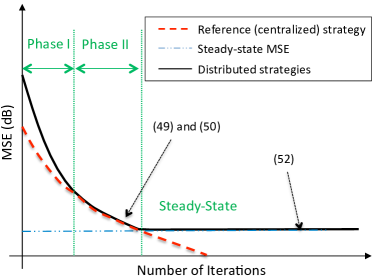
Figure 2: A typical mean-square-error (MSE) learning curve includes a transient stage that consists of two phases and a steady-state phase. The plot shows how the learning curve of a network of agents compares to the learning curve of a centralized reference solution. The analysis in this work, and in the accompanying Part II [44] characterizes in detail the parameters that determine the behavior of the network (rate, stability, and performance) during each phase of the learning process.

• Transient Phase I:
  If agents are initialized at different values, then the estimates of the various agents will initially evolve in such a way to make each $\bm{w}_{k,i}$ get closer to the reference recursion $\bar{w}_{c,i}$. The rate at which the agents approach $\bar{w}_{c,i}$ will be determined by $|\lambda_{2}(A)|$, the second largest eigenvalue of $A$ in magnitude. If the agents are initialized at the same value, say, e.g., $\bm{w}_{k,0}=0$, then the learning curves start at Transient Phase II directly.

• Transient Phase II:
  In this phase, the trajectories of all agents are uniformly close to the trajectory of the reference recursion; they converge in a coordinated manner to steady-state. The learning curves at this phase are well modeled by the same reference recursion (47) since we will show in (155) that:

  $$\mathbb{E}\|\tilde{\bm{w}}_{k,i}\|^{2}=\|\tilde{w}_{c,i}\|^{2}+O(\mu_{\max}^{1/2})\cdot\gamma_{c}^{i}+O(\mu_{\max})$$ (49)

  Furthermore, for small step-sizes and during the later stages of this phase, $\bar{w}_{c,i}$ will be close enough to $w^{o}$ and the convergence rate $r$ will be shown to satisfy:

  $$r =\big{[}\rho(I_{M}-\mu_{\max}H_{c})\big{]}^{2}+O\big{(}(\mu_{\max}\epsilon)^{\frac{1}{2(M-1)}}\big{)}$$ (50)

  where $\rho(\cdot)$ denotes the spectral radius of its matrix argument, $\epsilon$ is an arbitrarily small positive number, and $H_{c}$ is the same matrix that results from evaluating (29) at $w=w^{o}$, i.e.,

  $$H_{c}\triangleq\sum_{k=1}^{N}p_{k}H_{k}=H_{c}(w^{o})$$ (51)

  where $H_{k}\triangleq\nabla_{w^{T}}s_{k}(w^{o})$.

• Steady-State Phase:
  The reference recursion (47) continues converging towards $w^{o}$ so that $\|\tilde{w}_{c,i}\|^{2}=\|w^{o}-\bar{w}_{c,i}\|^{2}$ will converge to zero ($-\infty$ dB in Fig. 2). However, for the distributed strategy (1)–(3), the mean-square-error $\mathbb{E}\|\tilde{\bm{w}}_{k,i}\|^{2}=\mathbb{E}\|w^{o}-\bm{w}_{k,i}\|^{2}$ at each agent $k$ will converge to a finite steady-state value. We will be able to characterize this value in terms of the vector $p$ in Part II [44] as follows:

  $$\lim_{i\rightarrow\infty}\!\mathbb{E}\|\tilde{\bm{w}}_{k,i}\|^{2} =\mu_{\max}\!\cdot\!\mathrm{Tr}\left\{X(p^{T}\!\!\otimes\!I_{M})\mathcal{R}_{v}(p\!\otimes\!I_{M})\right\}$$

  $$\quad+o(\mu_{\max})$$ (52)

  where $X$ is the solution to the Lyapunov equation described later in (LABEL:P2-Equ:SteadyState:ContinuousLyapunovEqu_final) of Part II [44] (when $\Sigma=I$), and $o(\mu_{\max})$ denotes a strictly higher order term of $\mu_{\max}$. Expression (52) is a revealing result. It is a non-trivial extension of a classical result pertaining to the mean-square-error performance of stand-alone adaptive filters [54, 55, 56, 57] to the more demanding context when a multitude of adaptive agents are coupled together in a cooperative manner through a network topology. This result has an important ramification, which we pursue in Part II [44]. We will show there that no matter how the agents are connected to each other, there is always a way to select the combination weights such that the performance of the network is invariant to the topology. This will also imply that, for any connected topology, there is always a way to select the combination weights such that the performance of the network matches that of the centralized solution.

Note that the above results are obtained for the general distributed strategy (1)–(3). Therefore, the results can be specialized to the consensus, CTA diffusion, and ATC diffusion strategies in (10)–(12) by choosing the matrices $A_{1}$, $A_{2}$, and $A_{0}$ according to Tab. I. The results in this paper and its accompanying Part II[44] not only generalize the analysis from earlier works [16, 17, 19, 18, 20] but, more importantly, they also provide deeper insights into the learning behavior of these adaptation and learning strategies.

V Study of Error Dynamics

V-A Error Quantities

We shall examine the learning behavior of the distributed strategy (1)–(3) by examining how the perturbation between the distributed solution (1)–(3) and the reference solution (47) evolves over time — see Fig. 3. Specifically, let $\check{\bm{w}}_{k,i}$ denote the discrepancy between $\bm{w}_{k,i}$ and $\bar{w}_{c,i}$, i.e.,

$$\check{\bm{w}}_{k,i}\triangleq\bm{w}_{k,i}-\bar{w}_{c,i}$$ (53)

and let $\bm{w}_{i}$ and $\check{\bm{w}}_{i}$ denote the global vectors that collect the $\bm{w}_{k,i}$ and $\check{\bm{w}}_{k,i}$ from across the network, respectively:

$$\bm{w}_{i} \triangleq\mathrm{col}\{\bm{w}_{1,i},\ldots,\bm{w}_{N,i}\}$$ (54)

$$\check{\bm{w}}_{i} \triangleq\mathrm{col}\{\check{\bm{w}}_{1,i},\ldots,\check{\bm{w}}_{N,i}\}=\bm{w}_{i}-\mathds{1}\otimes\bar{w}_{c,i}$$ (55)

It turns out that it is insightful to study the evolution of $\check{\bm{w}}_{i}$ in a transformed domain where it is possible to express the distributed recursion (1)–(3) as a perturbed version of the reference recursion (47).

Definition 3 (Network basis transformation)

We define the transformation by introducing the Jordan canonical decomposition of the matrix $A=A_{1}A_{0}A_{2}$. Let

$$A^{T}=UDU^{-1}$$ (56)

where $U$ is an invertible matrix whose columns correspond to the right-eigenvectors of $A^{T}$, and $D$ is a block Jordan matrix with a single eigenvalue at one with multiplicity one while all other eigenvalues are strictly less than one. The Kronecker form of $A$ then admits the decomposition:

$$\mathcal{A}^{T}\triangleq A^{T}\otimes I_{M}=\mathcal{U}\mathcal{D}\mathcal{U}^{-1}$$ (57)

where

$$\mathcal{U} \triangleq U\otimes I_{M},\qquad\mathcal{D}\triangleq D\otimes I_{M}$$ (58)

We use $\mathcal{U}$ to define the following basis transformation:

$$\bm{w}_{i}^{\prime} \triangleq\mathcal{U}^{-1}\bm{w}_{i}=(U^{-1}\otimes I_{M})\bm{w}_{i}$$ (59)

$$\check{\bm{w}}_{i}^{\prime} \triangleq\mathcal{U}^{-1}\check{\bm{w}}_{i}=(U^{-1}\otimes I_{M})\check{\bm{w}}_{i}$$ (60)

The relations between the quantities in transformations (59)–(60) are illustrated in Fig. 3. ∎

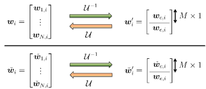
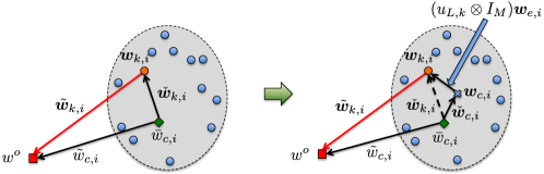
Figure 3: (a) Network basis transformation. (b) The diagrams show how the iterate $\bm{w}_{k,i}$ is decomposed relative to the reference $\bar{w}_{c,i}$ and relative to the centroid, $\bm{w}_{c,i}$, of the $N$ iterates across the network.

We can gain useful insight into the nature of this transformation by exploiting more directly the structure of the matrices $\mathcal{U}$, $\mathcal{D}$, and $\mathcal{U}^{-1}$. By Assumption 1, the matrix $A^{T}$ has an eigenvalue one of multiplicity one, with the corresponding left- and right-eigenvectors being $\theta^{T}$ and $\mathds{1}$, respectively. All other eigenvalues of $D$ are strictly less than one in magnitude. Therefore, the matrices $D$, $U$, and $U^{-1}$ can be partitioned as

$$D =\left[\begin{array}[]{c|c}1&\\ \hline\cr&D_{N-1}\end{array}\right]\quad U=\left[\begin{array}[]{c|c}\mathds{1}&U_{L}\end{array}\right]\quad U^{-1}=\left[\begin{array}[]{c}\theta^{T}\\ \hline\cr U_{R}\end{array}\right]$$ (66)

where $D_{N-1}$ is an $(N-1)\times(N-1)$ Jordan matrix with all diagonal entries strictly less than one in magnitude, $U_{L}$ is an $N\times(N-1)$ matrix, and $U_{R}$ is an $(N-1)\times N$ matrix. Then, the Kronecker forms $\mathcal{D}$, $\mathcal{U}$, and $\mathcal{U}^{-1}$ can be expressed as

$$\mathcal{D} =\left[\begin{array}[]{c|c}\!\!I_{M}\!\!&\\ \hline\cr&\!\!\mathcal{D}_{N\!-\!1}\!\!\end{array}\right],\;\mathcal{U}=\left[\begin{array}[]{c|c}\!\!\mathds{1}\!\otimes\!I_{M}\!\!&\!\!\mathcal{U}_{L}\!\!\end{array}\right],\;\mathcal{U}^{-1}=\left[\begin{array}[]{c}\!\!\theta^{T}\!\otimes\!I_{M}\!\!\\ \hline\cr\!\!\mathcal{U}_{R}\!\!\end{array}\right]$$ (72)

where

$$\mathcal{U}_{L} \triangleq U_{L}\otimes I_{M}$$ (73)

$$\mathcal{U}_{R} \triangleq U_{R}\otimes I_{M}$$ (74)

$$\mathcal{D}_{N-1} \triangleq D_{N-1}\otimes I_{M}$$ (75)

It is important to note that $U^{-1}U=I_{N}$ and that

$$\theta^{T}\mathds{1}=1,\quad\theta^{T}U_{L}=0,\quad U_{R}\mathds{1}=0,\quad U_{R}U_{L}=I_{N-1}$$ (76)

We first study the structure of $\bm{w}_{i}^{\prime}$ defined in (59) using (66):

$$\bm{w}_{i}^{\prime} =\mathrm{col}\{\underbrace{(\theta^{T}\otimes I_{M})\bm{w}_{i}}_{\triangleq\bm{w}_{c,i}},\;\underbrace{(U_{R}\otimes I_{M})\bm{w}_{i}}_{\triangleq\bm{w}_{e,i}}\}$$ (77)

The two components $\bm{w}_{c,i}$ and $\bm{w}_{e,i}$ have useful interpretations. Recalling that $\theta_{k}$ denotes the $k$th entry of the vector $\theta$, then $\bm{w}_{c,i}$ can be expressed as

$$\bm{w}_{c,i}=\sum_{k=1}^{N}\theta_{k}\bm{w}_{k,i}$$ (78)

As we indicated after Assumption 1, the entries $\{\theta_{k}\}$ are positive and add up to one. Therefore, $\bm{w}_{c,i}$ is a weighted average (i.e., the centroid) of the estimates $\{\bm{w}_{k,i}\}$ across all agents. To interpret $\bm{w}_{e,i}$, we examine the inverse mapping of (59) from $\bm{w}_{i}^{\prime}$ to $\bm{w}_{i}$ using the block structure of $\mathcal{U}$ in (66):

$$\bm{w}_{i} =(U\otimes I_{M})\bm{w}_{i}^{\prime}$$

$$=(\mathds{1}\otimes I_{M})\bm{w}_{c,i}+(U_{L}\otimes I_{M})\bm{w}_{e,i}$$

$$=\mathds{1}\otimes\bm{w}_{c,i}+(U_{L}\otimes I_{M})\bm{w}_{e,i}$$ (79)

which implies that the individual estimates at the various agents satisfy:

$$\bm{w}_{k,i}=\bm{w}_{c,i}+(u_{L,k}\otimes I_{M})\bm{w}_{e,i}$$ (80)

where $u_{L,k}$ denotes the $k$th row of the matrix $U_{L}$. The network basis transformation defined by (59) represents the cluster of iterates $\{\bm{w}_{k,i}\}$ by its centroid $\bm{w}_{c,i}$ and their positions $\{u_{L,k}\otimes I_{M})\bm{w}_{e,i}\}$ relative to the centroid as shown in Fig. 3. The two parts, $\bm{w}_{c,i}$ and $\bm{w}_{e,i}$, of $\bm{w}_{i}^{\prime}$ in (77) are the coordinates in this new transformed representation. Then, the actual error quantity $\tilde{\bm{w}}_{k,i}$ relative to $w^{o}$ can be represented as

$$\tilde{\bm{w}}_{k,i} =w^{o}-\bar{w}_{c,i}-(\bm{w}_{k,i}-\bar{w}_{c,i})$$

$$=w^{o}-\bar{w}_{c,i}-(\bm{w}_{c,i}+(u_{L,k}\otimes I_{M})\bm{w}_{e,i}-\bar{w}_{c,i})$$ (81)

Introduce

$$\tilde{w}_{c,i} \triangleq w^{o}-\bar{w}_{c,i}$$ (82)

$$\check{\bm{w}}_{c,i} \triangleq\bm{w}_{c,i}-\bar{w}_{c,i}$$ (83)

Then, from (81) we arrive at the following critical relation for our analysis in the sequel:

$$\tilde{\bm{w}}_{k,i} =\tilde{w}_{c,i}-\check{\bm{w}}_{c,i}-(u_{L,k}\otimes I_{M})\bm{w}_{e,i}$$ (84)

This relation is also illustrated in Fig. 3. Then, the behavior of the error quantities $\{\tilde{\bm{w}}_{k,i}\}$ can be studied by examining $\tilde{w}_{c,i}$, $\check{\bm{w}}_{c,i}$ and $\bm{w}_{e,i}$, respectively, which is pursued in Sec. VI further ahead. The first term is the error between the reference recursion and $w^{o}$, which is studied in Theorems 1–3. The second quantity is the difference between the weighted centroid $\bm{w}_{c,i}$ of the cluster and the reference vector $\bar{w}_{c,i}$, and the third quantity characterizes the positions of the individual iterates $\{\bm{w}_{k,i}\}$ relative to the centroid $\bm{w}_{c,i}$. As long as the second and the third terms in (84), or equivalently, $\check{\bm{w}}_{c,i}$ and $\bm{w}_{e,i}$, are small (which will be shown in Theorem 4), the behavior of each $\bm{w}_{k,i}$ can be well approximated by the behavior of the reference vector $\bar{w}_{c,i}$. Indeed, $\check{\bm{w}}_{c,i}$ and $\bm{w}_{e,i}$ are the coordinates of the transformed vector $\check{\bm{w}}_{i}^{\prime}$ defined by (60). To see this, we substitute (66) and (55) into (60) to get

$$\check{\bm{w}}_{i}^{\prime} =(U^{-1}\otimes I_{M})(\bm{w}_{i}-\mathds{1}\otimes\bar{w}_{c,i})$$

$$=\bm{w}_{i}^{\prime}-(U^{-1}\mathds{1})\otimes\bar{w}_{c,i}$$ (85)

Recalling (76) and the expression for $U^{-1}$ in (66), we obtain

$$U^{-1}\mathds{1} =\mathrm{col}\{\theta^{T}\mathds{1},\;U_{R}\mathds{1}\}$$

$$=\mathrm{col}\{1,\;0_{N-1}\}$$ (86)

where $0_{N-1}$ denotes an $(N-1)\times 1$ vector with all zero entries. Substituting (86) and (77) into (85), we get

$$\check{\bm{w}}_{i}^{\prime}=\mathrm{col}\{\bm{w}_{c,i}-\bar{w}_{c,i},\;\bm{w}_{e,i}\}=\mathrm{col}\{\check{\bm{w}}_{c,i},\;\bm{w}_{e,i}\}$$ (87)

Therefore, it suffices to study the dynamics of $\check{\bm{w}}_{i}^{\prime}$ and its mean-square performance. We will establish joint recursions for $\bm{w}_{c,i}$ and $\bm{w}_{e,i}$ in Sec. V-B, and joint recursions for $\check{\bm{w}}_{c,i}$ and $\bm{w}_{e,i}$ in Sec. V-C. Table II summarizes the definitions of the various quantities, the recursions that they follow, and their relations.

TABLE II: Summary of various iterates, error quantities, and their relations.

	Original system			Transformed systema			Reference system
Quantity	$\bm{w}_{k,i}$	$\tilde{\bm{w}}_{k,i}$	$\check{\bm{w}}_{k,i}$	$\bm{w}_{c,i}$	$\check{\bm{w}}_{c,i}$	$\bm{w}_{e,i}$	$\bar{w}_{c,i}$	$\tilde{w}_{c,i}$
Definition	Iterate at agent $k$	$w^{o}\!-\!\bm{w}_{k,i}$	$\bm{w}_{k,i}\!-\!\bar{w}_{c,i}$	$\displaystyle\sum_{k=1}^{N}\theta_{k}\bm{w}_{k,i}$	$\bm{w}_{c,i}\!-\!\bar{w}_{c,i}$	$\mathcal{U}_{R}\bm{w}_{i}$	Ref. Iterate	$w^{o}\!-\!\bar{w}_{c,i}$
Recursion	Eqs. (1)–(3)	Nothing	Nothing	Eq. (106)	Eq. (113)	Eq. (114)	Eq. (47)	Nothing

• The transformation is defined by (59)–(60).

V-B Signal Recursions

We now derive the joint recursion that describes the evolution of the quantities $\check{\bm{w}}_{c,i}=\bm{w}_{c,i}-\bar{w}_{c,i}$ and $\bm{w}_{e,i}$. Since $\bar{w}_{c,i}$ follows the reference recursion (47), it suffices to derive the joint recursion for $\bm{w}_{c,i}$ and $\bm{w}_{e,i}$. To begin with, we introduce the following global quantities:

$$\mathcal{A} =A\otimes I_{M}$$ (88)

$$\mathcal{A}_{0} =A_{0}\otimes I_{M}$$ (89)

$$\mathcal{A}_{1} =A_{1}\otimes I_{M}$$ (90)

$$\mathcal{A}_{2} =A_{2}\otimes I_{M}$$ (91)

$$\mathcal{M} =\Omega\otimes I_{M}$$ (92)

$$\Omega =\mathrm{diag}\{\mu_{1},\ldots,\mu_{N}\}$$ (93)

We also let the notation $x=\mathrm{col}\{x_{1},\ldots,x_{N}\}$ denote an arbitrary $N\times 1$ block column vector that is formed by stacking $M\times 1$ sub-vectors $x_{1},\ldots,x_{N}$ on top of each other. We further define the following global update vectors:

$$\hat{\bm{s}}_{i}(x) \triangleq\mathrm{col}\{\hat{\bm{s}}_{1,i}(x_{1}),\ldots,\hat{\bm{s}}_{N,i}(x_{N})\}$$ (94)

$$s(x) \triangleq\mathrm{col}\{s_{1}(x_{1}),\ldots,s_{N}(x_{N})\}$$ (95)

Then, the general recursion for the distributed strategy (1)–(3) can be rewritten in terms of these extended quantities as follows:

$$\bm{w}_{i}=\mathcal{A}^{T}\bm{w}_{i-1}-\mathcal{A}_{2}^{T}\mathcal{M}\hat{\bm{s}}_{i}(\bm{\phi}_{i-1})$$ (96)

where

$$\bm{\phi}_{i}\triangleq\mathrm{col}\{\bm{\phi}_{1,i},\ldots,\bm{\phi}_{N,i}\}$$ (97)

and is related to $\bm{w}_{i}$ and $\bm{w}_{i}^{\prime}$ via the following relation

$$\bm{\phi}_{i}=\mathcal{A}_{1}^{T}\bm{w}_{i}=\mathcal{A}_{1}^{T}\mathcal{U}\bm{w}_{i}^{\prime}$$ (98)

Applying the transformation (59) to both sides of (96), we obtain the transformed global recursion:

$$\bm{w}_{i}^{\prime}=\mathcal{D}\bm{w}_{i-1}^{\prime}-\mathcal{U}^{-1}\mathcal{A}_{2}^{T}\mathcal{M}\hat{\bm{s}}_{i}\left(\bm{\phi}_{i-1}\right)$$ (99)

We can now use the block structures in (72) and (77) to derive recursions for $\bm{w}_{c,i}$ and $\bm{w}_{e,i}$ from (99). Substituting (72) and (77) into (99), and using properties of Kronecker products[58, p.147], we obtain

$$\bm{w}_{c,i} =\bm{w}_{c,i-1}-(\theta^{T}\otimes I_{M})\mathcal{A}_{2}^{T}\mathcal{M}\hat{\bm{s}}_{i}\left(\bm{\phi}_{i-1}\right)$$

$$=\bm{w}_{c,i-1}-(\theta^{T}A_{2}^{T}\Omega\otimes I_{M})\hat{\bm{s}}_{i}\left(\bm{\phi}_{i-1}\right)$$

$$=\bm{w}_{c,i-1}-\mu_{\max}\cdot(p^{T}\otimes I_{M})\hat{\bm{s}}_{i}\left(\bm{\phi}_{i-1}\right)$$ (100)

and

$$\bm{w}_{e,i} =\mathcal{D}_{N-1}\bm{w}_{e,i-1}-\mathcal{U}_{R}\mathcal{A}_{2}^{T}\mathcal{M}\hat{\bm{s}}_{i}\left(\bm{\phi}_{i-1}\right)$$ (101)

where in the last step of (100) we used the relation

$$\mu_{\max}\cdot p=\Omega A_{2}\theta$$ (102)

which follows from Definitions 1 and 2. Furthermore, by adding and subtracting identical factors, the term $\hat{\bm{s}}_{i}\left(\bm{\phi}_{i-1}\right)$ that appears in (100) and (101) can be expressed as

$$\hat{\bm{s}}_{i}\left(\bm{\phi}_{i-1}\right) =s(\mathds{1}\otimes\bm{w}_{c,i-1})+\underbrace{\hat{\bm{s}}_{i}\left(\bm{\phi}_{i-1}\right)\!-\!s\left(\bm{\phi}_{i-1}\right)}_{\triangleq\bm{v}_{i}(\bm{\phi}_{i-1})}$$

$$\quad+\underbrace{s\left(\bm{\phi}_{i-1}\right)\!-\!s(\mathds{1}\otimes\bm{w}_{c,i-1})}_{\triangleq\bm{z}_{i-1}}$$ (103)

where the first perturbation term $\bm{v}_{i}(\bm{\phi}_{i-1})$ consists of the difference between the true update vectors $\{s_{k}(\bm{\phi}_{k,i-1})\}$ and their stochastic approximations $\{\hat{\bm{s}}_{k,i}(\bm{\phi}_{k,i-1})\}$, while the second perturbation term $\bm{z}_{i-1}$ represents the difference between the same $\{s_{k}(\bm{\phi}_{k,i-1})\}$ and $\{s_{k}(\bm{w}_{c,i-1})\}$. The subscript $i-1$ in $\bm{z}_{i-1}$ implies that this variable depends on data up to time $i-1$ and the subscript $i$ in $\bm{v}_{i}(\bm{\phi}_{i-1})$ implies that its value depends on data up to time $i$ (since, in general, $\hat{\bm{s}}_{i}(\cdot)$ can depend on data from time $i$ — see Eq. (LABEL:P2-Equ:Example:ski_LMS) in Part II for an example). Then, $\hat{\bm{s}}_{i}\left(\bm{\phi}_{i-1}\right)$ can be expressed as

$$\hat{\bm{s}}_{i}\left(\bm{\phi}_{i-1}\right) =s(\mathds{1}\otimes\bm{w}_{c,i-1})+\bm{v}_{i}+\bm{z}_{i-1}$$ (104)

Lemma 2 (Signal dynamics)

In summary, the previous derivation shows that the weight iterates at each agent evolve according to the following dynamics:

$$\bm{w}_{k,i} =\bm{w}_{c,i}+(u_{L,k}\otimes I_{M})\bm{w}_{e,i}$$ (105)

$$\bm{w}_{c,i} =\bm{w}_{c,i-1}-\mu_{\max}\cdot(p^{T}\otimes I_{M})\hat{\bm{s}}_{i}\left(\bm{\phi}_{i-1}\right)$$ (106)

$$\bm{w}_{e,i} =\mathcal{D}_{N-1}\bm{w}_{e,i-1}-\mathcal{U}_{R}\mathcal{A}_{2}^{T}\mathcal{M}\hat{\bm{s}}_{i}\left(\bm{\phi}_{i-1}\right)$$ (107)

$$\hat{\bm{s}}_{i}\left(\bm{\phi}_{i-1}\right) =s(\mathds{1}\otimes\bm{w}_{c,i-1})+\bm{v}_{i}+\bm{z}_{i-1}$$ (108)

∎

V-C Error Dynamics

To simplify the notation, we introduce the centralized operator $T_{c}:\mathbb{R}^{M}\rightarrow\mathbb{R}^{M}$ as the following mapping for any $x\in\mathbb{R}^{M}$:

$$T_{c}(x) \triangleq x-\mu_{\max}\cdot(p^{T}\otimes I_{M})\;s(\mathds{1}\otimes x)$$

$$=x-\mu_{\max}\sum_{k=1}^{N}p_{k}s_{k}(x)$$ (109)

Substituting (104) into (106)–(107) and using (109), we find that we can rewrite (106) and (107) in the alternative form:

$$\bm{w}_{c,i} =T_{c}(\bm{w}_{c,i-1})-\mu_{\max}\cdot(p^{T}\otimes I_{M})\left[\bm{z}_{i-1}+\bm{v}_{i}\right]$$ (110)

$$\bm{w}_{e,i} =\mathcal{D}_{N-1}\bm{w}_{e,i-1}-\mathcal{U}_{R}\mathcal{A}_{2}^{T}\mathcal{M}\left[s(\mathds{1}\otimes\bm{w}_{c,i-1})+\bm{z}_{i-1}\!+\!\bm{v}_{i}\right]$$ (111)

Likewise, we can write the reference recursion (47) in the following compact form:

$$\bar{w}_{c,i}=T_{c}(\bar{w}_{c,i-1})$$ (112)

Comparing (110) with (112), we notice that the recursion for the centroid vector, $\bm{w}_{c,i}$, follows the same update rule as the reference recursion except for the two driving perturbation terms $\bm{z}_{i-1}$ and $\bm{v}_{i}$. Therefore, we would expect the trajectory of $\bm{w}_{c,i}$ to be a perturbed version of that of $\bar{w}_{c,i}$. Recall from (83) that

$$\check{\bm{w}}_{c,i}\triangleq\bm{w}_{c,i}-\bar{w}_{c,i}$$

To obtain the dynamics of $\check{\bm{w}}_{c,i}$, we subtract (112) from (110).

Lemma 3 (Error dynamics)

The error quantities that appear on the right-hand side of (87) evolve according to the following dynamics:

$$\check{\bm{w}}_{c,i} =T_{c}(\bm{w}_{c,i-1})-T_{c}(\bar{w}_{c,i-1})$$

$$\quad-\mu_{\max}\!\cdot\!(p^{T}\!\otimes\!I_{M})\left[\bm{z}_{i-1}+\bm{v}_{i}\right]$$ (113)

$$\bm{w}_{e,i} =\mathcal{D}_{N-1}\bm{w}_{e,i-1}$$

$$\quad-\mathcal{U}_{R}\mathcal{A}_{2}^{T}\mathcal{M}\left[s(\mathds{1}\otimes\bm{w}_{c,i-1})\!+\!\bm{z}_{i-1}\!+\!\bm{v}_{i}\right]$$ (114)

∎

The analysis in sequel will study the dynamics of the variances of the error quantities $\check{\bm{w}}_{c,i}$ and ${\bm{w}}_{e,i}$ based on (113)–(114). The main challenge is that these two recursions are coupled with each other through $\bm{z}_{i-1}$ and $\bm{v}_{i}$. To address the difficulty, we will extend the energy operator approach developed in [20] to the general scenario under consideration.

V-D Energy Operators

To carry out the analysis, we need to introduce the following operators.

Definition 4 (Energy vector operator)

Suppose $x=\mathrm{col}\{x_{1},\ldots,x_{N}\}$ is an arbitrary $N\times 1$ block column vector that is formed by stacking $M_{0}\times 1$ vectors $x_{1},\ldots,x_{N}$ on top of each other. The energy vector operator $P_{M_{0}}:\mathbb{C}^{M_{0}N}\rightarrow\mathbb{R}^{N}$ is defined as the mapping:

$$P_{M_{0}}[x]\triangleq\mathrm{col}\{\|x_{1}\|^{2},\ldots,\|x_{N}\|^{2}\}$$ (115)

where $\|\cdot\|$ denotes the Euclidean norm of a vector. ∎

Definition 5 (Norm matrix operator)

Suppose $X$ is an arbitrary $K\times N$ block matrix consisting of blocks $\{X_{kn}\}$ of size $M_{0}\times M_{0}$:

$$X =\begin{bmatrix}X_{11}&\cdots&X_{1N}\\ \vdots&&\vdots\\ X_{K1}&\cdots&X_{KN}\end{bmatrix}$$ (116)

The norm matrix operator $\bar{P}_{M_{0}}:\mathbb{C}^{M_{0}K\times M_{0}N}\rightarrow\mathbb{R}^{K\times N}$ is defined as the mapping:

$$\bar{P}_{M_{0}}[x]\triangleq\begin{bmatrix}\|X_{11}\|&\cdots&\|X_{1N}\|\\ \vdots&&\vdots\\ \|X_{K1}\|&\cdots&\|X_{KN}\|\end{bmatrix}$$ (117)

where $\|\cdot\|$ denotes the $2-$induced norm of a matrix. ∎

By default, we choose $M_{0}$ to be $M$, the size of the vector $\bm{w}_{k,i}$. In this case, we will drop the subscript in$P_{M_{0}}[\cdot]$ and use $P[\cdot]$ for convenience. However, in other cases, we will keep the subscript to avoid confusion. Likewise, $\bar{P}_{M_{0}}[\cdot]$ characterizes the norms of different parts of a matrix it operates on. We will also drop the subscript if $M_{0}=M$. In Appendix A, we collect several properties of the above energy operators, and which will be used in the sequel to characterize how the energy of the error quantities propagates through the dynamics (113)–(114).

VI Transient Analysis

Using the energy operators and the various properties, we can now examine the transient behavior of the learning curve more closely. Recall from (84) that $\tilde{\bm{w}}_{k,i}$ consists of three parts: the error of the reference recursion, $\tilde{w}_{c,i}$, the difference between the centroid and the reference, $\check{\bm{w}}_{c,i}$, and the position of individual iterates relative to the centroid, $(u_{L,k}\otimes I_{M})\bm{w}_{e,i}$. The main objective in the sequel is to study the convergence of the reference error, $\tilde{w}_{c,i}$, and establish non-asymptotic bounds for the mean-square values of $\check{\bm{w}}_{c,i}$ and $\bm{w}_{e,i}$, which will allow us to understand how fast and how close the iterates at the individual agents, $\{\bm{w}_{k,i}\}$, get to the reference recursion. Recalling from (87) that $\check{\bm{w}}_{c,i}$ and $\bm{w}_{e,i}$ are the two blocks of the transformed vector $\check{\bm{w}}_{i}^{\prime}$ defined by (60), we can examine instead the evolution of

$$\check{\mathcal{W}}_{i}^{\prime} \triangleq\mathbb{E}P[\check{\bm{w}}_{i}^{\prime}]=\mathrm{col}\left\{\mathbb{E}P[\check{\bm{w}}_{c,i}],\mathbb{E}P[\bm{w}_{e,i}]\right\}$$

$$=\mathrm{col}\left\{\mathbb{E}\|\check{\bm{w}}_{c,i}\|^{2},\mathbb{E}P[\bm{w}_{e,i}]\right\}$$ (118)

Specifically, we will study the convergence of $\tilde{w}_{c,i}$ in Sec. VI-A, the stability of $\check{\mathcal{W}}_{i}^{\prime}$ in Sec. VI-B, and the two transient phases of $\tilde{\bm{w}}_{k,i}$ in Sec. VI-C.

VI-A Limit Point

Before we proceed to study $\check{\mathcal{W}}_{i}^{\prime}$, we state the following theorems on the existence of a limit point and on the convergence of the reference recursion (112).

Theorem 1 (Limit point)

Given Assumptions 3–4, there exists a unique $M\times 1$ vector $w^{o}$ that solves

$$\sum_{k=1}^{N}p_{k}s_{k}(w^{o})=0$$ (119)

where $p_{k}$ is the $k$th entry of the vector $p$ defined in (16).

Proof:

See Appendix E. ∎

Theorem 2 (Convergence of the reference recursion)

Let $\tilde{w}_{c,i}\triangleq w^{o}-\bar{w}_{c,i}$ denote the error vector of the reference recursion (112). Then, the following non-asymptotic bound on the squared error holds for all $i\geq 0$:

$$(1\!-\!2\mu_{\max}\|p\|_{1}\lambda_{U})^{i}\!\cdot\!\|\tilde{w}_{c,0}\|^{2}\leq\|\tilde{w}_{c,i}\|^{2}\leq\gamma_{c}^{2i}\!\cdot\!\|\tilde{w}_{c,0}\|^{2}$$ (120)

where

$$\gamma_{c}\triangleq 1-\mu_{\max}\lambda_{L}+\frac{1}{2}\mu_{\max}^{2}\|p\|_{1}^{2}\lambda_{U}^{2}$$ (121)

Furthermore, if the following condition on the step-size holds

$$0<\mu_{\max}<\frac{2\lambda_{L}}{\|p\|_{1}^{2}\lambda_{U}^{2}}$$ (122)

then, the iterate $\tilde{w}_{c,i}$ converges to zero.

Proof:

See Appendix F. ∎

Note from (120) that, when the step-size is sufficiently small, the reference recursion (47) converges at a geometric rate between $1-2\mu_{\max}\|p\|_{1}\lambda_{U}$ and $\gamma_{c}^{2}=1-2\mu_{\max}\lambda_{L}+o(\mu_{\max})$. Note that this is a non-asymptotic result. That is, the convergence rate $r_{\mathrm{Ref}}$ of the reference recursion (112) is always lower and upper bounded by these two rates:

$$1-2\mu_{\max}\|p\|_{1}\lambda_{U}\leq r_{\mathrm{Ref}}\leq\gamma_{c}^{2},\quad\forall i\geq 0$$ (123)

We can obtain a more precise characterization of the convergence rate of the reference recursion in the asymptotic regime (for large enough $i$), as follows.

Theorem 3 (Convergence rate of the reference recursion)

Specifically, for any small $\epsilon>0$, there exists a time instant $i_{0}$ such that, for $i\geq i_{0}$, the error vector $\tilde{w}_{c,i}$ converges to zero at the following rate:

$$r_{\mathrm{Ref}} =\big{[}\rho(I_{M}-\mu_{\max}H_{c})\big{]}^{2}+O\big{(}(\mu_{\max}\epsilon)^{\frac{1}{2(M-1)}}\big{)}$$ (124)

Proof:

See Appendix G. ∎

Note that since (124) holds for arbitrary $\epsilon>0$, we can choose $\epsilon$ to be an arbitrarily small positive number. Therefore, the convergence rate of the reference recursion is arbitrarily close to $[\rho(I_{M}-\mu_{\max}H_{c})]^{2}$.

VI-B Mean-Square Stability

Now we apply the properties from Lemmas 5–6 to derive an inequality recursion for the transformed energy vector $\check{\mathcal{W}}_{i}^{\prime}=\mathbb{E}P[\check{\bm{w}}_{i}^{\prime}]$. The results are summarized in the following lemma.

Lemma 4 (Inequality recursion for $\check{\mathcal{W}}_{i}^{\prime}$)

The $N\times 1$ vector $\check{\mathcal{W}}_{i}^{\prime}$ defined by (118) satisfies the following relation for all time instants:

$$\check{\mathcal{W}}_{i}^{\prime}\preceq\Gamma\check{\mathcal{W}}_{i-1}^{\prime}+\mu_{\max}^{2}b_{v}$$ (125)

where

$$\Gamma \triangleq\Gamma_{0}+\mu_{\max}^{2}\psi_{0}\cdot\mathds{1}\mathds{1}^{T}\in\mathbb{R}^{N\times N}$$ (126)

$$\Gamma_{0} \triangleq\begin{bmatrix}\gamma_{c}&\mu_{\max}h_{c}(\mu_{\max})\cdot\mathds{1}^{T}\\ 0&\Gamma_{e}\end{bmatrix}\in\mathbb{R}^{N\times N}$$ (127)

$$b_{v} \triangleq\mathrm{col}\{b_{v,c},\;b_{v,e}\cdot\mathds{1}\}\in\mathbb{R}^{N}$$ (128)

$$\Gamma_{e} \triangleq\begin{bmatrix}|\lambda_{2}(A)|&\frac{2}{1-|\lambda_{2}(A)|}&&\\ &\ddots&\ddots&\\ &\!\!&\ddots&\frac{2}{1-|\lambda_{2}(A)|}\\ &&&|\lambda_{2}(A)|\end{bmatrix}\!\in\mathbb{R}^{(N\!-\!1)\times(N\!-\!1)}$$ (129)

The scalars $\psi_{0}$, $h_{c}(\mu)$, $b_{v,c}$ and $b_{v,e}$ are defined as

$$\psi_{0} \triangleq\max\bigg{\{}4\alpha\|p\|_{1}^{2},\;\;4\alpha\|p\|_{1}^{2}\cdot\left\|\bar{P}[\mathcal{A}_{1}^{T}\mathcal{U}_{L}]\right\|_{\infty}^{2},\;\;$$

$$\qquad 4N\cdot\left\|\bar{P}[\mathcal{U}_{R}\mathcal{A}_{2}^{T}]\right\|_{\infty}^{2}\lambda_{U}^{2}\left(\frac{3}{1-|\lambda_{2}(A)|}+\frac{\alpha}{\lambda_{U}^{2}}\right),$$

$$\qquad 4N\cdot\left\|\bar{P}[\mathcal{U}_{R}\mathcal{A}_{2}^{T}]\right\|_{\infty}^{2}\cdot\left\|\bar{P}[\mathcal{A}_{1}^{T}\mathcal{U}_{L}]\right\|_{\infty}^{2}\lambda_{U}^{2}$$

$$\qquad\cdot\left(\frac{1}{1-|\lambda_{2}(A)|}+\frac{\alpha}{\lambda_{U}^{2}}\right)\bigg{\}}$$ (130)

$$h_{c}(\mu_{\max}) \triangleq\|p\|_{1}^{2}\!\cdot\!\left\|\bar{P}[\mathcal{A}_{1}^{T}\mathcal{U}_{L}]\right\|_{\infty}^{2}\lambda_{U}^{2}\!\cdot\!\Big{[}\frac{1}{\lambda_{L}\!-\!\frac{1}{2}\mu_{\max}\|p\|_{1}^{2}\lambda_{U}^{2}}\Big{]}$$ (131)

$$b_{v,c} \triangleq\|p\|_{1}^{2}\cdot\left[4\alpha(\|\tilde{w}_{c,0}\|^{2}+\|w^{o}\|^{2})+\sigma_{v}^{2}\right]$$ (132)

$$b_{v,e} \triangleq N\left\|\bar{P}[\mathcal{U}_{R}\mathcal{A}_{2}^{T}]\right\|_{\infty}^{2}\bigg{(}12\frac{\lambda_{U}^{2}\|\tilde{w}_{c,0}\|^{2}+\|g^{o}\|_{\infty}}{1-|\lambda_{2}(A)|}$$

$$\qquad+4\alpha(\|\tilde{w}_{c,0}\|^{2}+\|w^{o}\|^{2})+\sigma_{v}^{2}\bigg{)}$$ (133)

where $g^{o}\triangleq P[s(\mathds{1}\otimes w^{o})]$.

Proof:

See Appendix H. ∎

From (126)–(127), we see that as the step-size $\mu_{\max}$ becomes small, we have $\Gamma\approx\Gamma_{0}$, since the second term in the expression for $\Gamma$ depends on the square of the step-size. Moreover, note that $\Gamma_{0}$ is an upper triangular matrix. Therefore, $\check{\bm{w}}_{c,i}$ and $\bm{w}_{e,i}$ are weakly coupled for small step-sizes; $\mathbb{E}P[\bm{w}_{e,i}]$ evolves on its own, but it will seep into the evolution of $\mathbb{E}P[\check{\bm{w}}_{c,i}]$ via the off-diagonal term in $\Gamma_{0}$, which is $O(\mu_{\max})$. This insight is exploited to establish a non-asymptotic bound on $\check{\mathcal{W}}_{i}^{\prime}=\mathrm{col}\{\mathbb{E}\|\check{\bm{w}}_{c,i}\|^{2},\mathbb{E}P[\bm{w}_{e,i}]\}$ in the following theorem.

Theorem 4 (Non-asymptotic bound for $\check{\mathcal{W}}_{i}^{\prime}$)

Suppose the matrix $\Gamma$ defined in (126) is stable, i.e., $\rho(\Gamma)<1$. Then, the following non-asymptotic bound holds for all $i\geq 0$:

$$\mathbb{E}P[\check{\bm{w}}_{c,i}] \preceq\mu_{\max}h_{c}(\mu_{\max})\!\cdot\!\mathds{1}^{T}(\gamma_{c}I\!-\!\Gamma_{e})^{-1}\left(\gamma_{c}^{i}I\!-\!\Gamma_{e}^{i}\right)\mathcal{W}_{e,0}$$

$$\quad+\check{\mathcal{W}}_{c,\infty}^{\mathrm{ub}^{\prime}}$$ (134)

$$\mathbb{E}P[\bm{w}_{e,i}] \preceq\Gamma_{e}^{i}\mathcal{W}_{e,0}+\check{\mathcal{W}}_{e,\infty}^{\mathrm{ub}^{\prime}}$$ (135)

where $\mathcal{W}_{e,0}\triangleq\mathbb{E}P[\bm{w}_{e,0}]$, $\check{\mathcal{W}}_{c,\infty}^{\mathrm{ub}^{\prime}}$ and $\check{\mathcal{W}}_{e,\infty}^{\mathrm{ub}^{\prime}}$ are the $\limsup$ bounds of $\mathbb{E}P[\check{\bm{w}}_{c,i}]$ and $\mathbb{E}P[\bm{w}_{e,i}]$, respectively:

$$\check{\mathcal{W}}_{c,\infty}^{\mathrm{ub}^{\prime}} =\mu_{\max}\cdot\frac{\psi_{0}\big{(}\lambda_{L}+h_{c}(0)\big{)}\mathds{1}^{T}(I-\Gamma_{e})^{-1}\mathcal{W}_{e,0}+b_{v,c}\lambda_{L}}{\lambda_{L}^{2}}$$

$$\quad+o(\mu_{\max})$$ (136)

$$\check{\mathcal{W}}_{e,\infty}^{\mathrm{ub}^{\prime}} =\mu_{\max}^{2}\!\cdot\!\frac{\psi_{0}\big{(}\lambda_{L}+h_{c}(0)\big{)}\mathds{1}^{T}(I-\Gamma_{e})^{-1}\mathcal{W}_{e,0}+b_{v,e}\lambda_{L}}{\lambda_{L}}$$

$$\quad\times(I\!-\!\Gamma_{e})^{-\!1}\mathds{1}+o(\mu_{\max}^{2})$$ (137)

where $o(\cdot)$ denotes strictly higher order terms, and $h_{c}(0)$ is the value of $h_{c}(\mu_{\max})$ (see (131)) evaluated at $\mu_{\max}=0$. An important implication of (134) and (136) is that

$$\mathbb{E}P[\check{\bm{w}}_{c,i}]\leq O(\mu_{\max}),\qquad\quad\forall i\geq 0$$ (138)

Furthermore, a sufficient condition that guarantees the stability of the matrix $\Gamma$ is that

$$0<\mu_{\max}<\min\bigg{\{}\!\! \frac{\lambda_{L}}{\frac{1}{2}\|p\|_{1}^{2}\lambda_{U}^{2}\!+\!\frac{1}{3}\psi_{0}\left(\!\frac{1-|\lambda_{2}(A)|}{2}\!\right)^{\!-2N}},\;$$

$$\sqrt{\frac{3(1\!-\!|\lambda_{2}(A)|)^{2N\!+\!1}}{2^{2N+2}\psi_{0}}},\;$$

$$\frac{\lambda_{L}}{\|p\|_{1}^{2}\lambda_{U}^{2}\!\left(\|\bar{P}_{1}[A^{T}U_{L}]\|_{\infty}^{2}\!+\!\frac{1}{2}\right)}\!\!\bigg{\}}$$ (139)

Proof:

See Appendix J. ∎

Corollary 1 (Asymptotic bounds)

It holds that

$$\limsup_{i\rightarrow\infty}\mathbb{E}\|\check{\bm{w}}_{c,i}\|^{2} \leq O(\mu_{\max})$$ (140)

$$\limsup_{i\rightarrow\infty}\mathbb{E}\|\bm{w}_{e,i}\|^{2} \leq O(\mu_{\max}^{2})$$ (141)

Proof:

The bound (140) holds since $\mathbb{E}\|\check{\bm{w}}_{c,i}\|^{2}=\mathbb{E}P[\check{\bm{w}}_{c,i}]\leq O(\mu_{\max})$ for all $i\geq 0$ according to (138). Furthermore, inequality (141) holds because

$$\limsup_{i\rightarrow\infty}\mathbb{E}\|\bm{w}_{e,i}\|^{2} \overset{(a)}{=}\limsup_{i\rightarrow\infty}\mathds{1}^{T}\mathbb{E}P[\bm{w}_{e,i}]$$

$$\overset{(b)}{\preceq}\mathds{1}^{T}\check{\mathcal{W}}_{e,\infty}^{\mathrm{ub}^{\prime}}$$

$$\overset{(c)}{=}O(\mu_{\max}^{2})$$ (142)

where step (a) uses property (167) of the energy operator $P[\cdot]$, step (b) uses (135), and step (c) uses (137). ∎

Finally, we present following main theorem that characterizes the difference between the learning curve of $\tilde{\bm{w}}_{k,i}$ at each agent $k$ and that of $\tilde{w}_{c,i}$ generated by the reference recursion (112).

Theorem 5 (Learning behavior of $\mathbb{E}\|\tilde{\bm{w}}_{k,i}\|^{2}$)

Suppose the stability condition (139) holds. Then, the difference between the learning curve of the mean-square-error $\mathbb{E}\|\tilde{\bm{w}}_{k,i}\|^{2}$ at each agent $k$ and the learning curve of $\|\tilde{w}_{c,i}\|^{2}$ is bounded non-asymptotically as

$$\big{|}\mathbb{E} \|\tilde{\bm{w}}_{k,i}\|^{2}-\|\tilde{w}_{c,i}\|^{2}\big{|}$$

$$\leq 2\|u_{L,k}\otimes I_{M}\|^{2}\cdot\mathds{1}^{T}\Gamma_{e}^{i}\mathcal{W}_{e,0}$$

$$\quad+2\|\tilde{w}_{c,0}\|\cdot\|u_{L,k}\otimes I_{M}\|\cdot\sqrt{\mathds{1}^{T}\Gamma_{e}^{i}\mathcal{W}_{e,0}}$$

$$\quad+\gamma_{c}^{i}\cdot O(\mu_{\max}^{\frac{1}{2}})+O(\mu_{\max})\qquad\quad\mathrm{for~{}all~{}}i\geq 0$$ (143)

where $\gamma_{c}$ was defined earlier in (121).

Proof:

See Appendix L. ∎

VI-C Interpretation of Results

TABLE III: Behavior of error quantities in different phases.

Error quantity	Transient Phase I		Transient Phase II		Steady-State c
	Convergence rate $r$   a	Value	Convergence rate $r$    b	Value	Value
$\|\tilde{w}_{c,i}\|^{2}$	$1-2\mu_{\max}\|p\|_{1}\lambda_{U}\leq r\leq\gamma_{c}^{2}$	$\gg O(\mu_{\max})$	$r=[\rho(I_{M}-\mu_{\max}H_{c})]^{2}$	$\gg O(\mu_{\max})$	0
$\mathbb{E}\|\check{\bm{w}}_{c,i}\|^{2}$	converged	$O(\mu_{\max})$	converged	$O(\mu_{\max})$	$O(\mu_{\max})$
$\mathbb{E}P[\check{\bm{w}}_{e,i}]$	$r\leq|\lambda_{2}(A)|$	$\gg O(\mu_{\max})$	converged	$O(\mu_{\max}^{2})$	$O(\mu_{\max}^{2})$
$\mathbb{E}\|\tilde{\bm{w}}_{k,i}\|^{2}$	Multiple modes	$\gg O(\mu_{\max})$	$r=[\rho(I_{M}-\mu_{\max}H_{c})]^{2}$	$\gg O(\mu_{\max})$	$O(\mu_{\max})$

• $\gamma_{c}$ is defined in (121), and $\gamma_{c}^{2}=1-2\mu_{\max}\lambda_{L}+o(\mu_{\max})$.

• We only show the leading term of the convergence rate for $r$. More precise expression can be found in (124).

• Closer studies of the steady-state performance can be found in Part II [44].

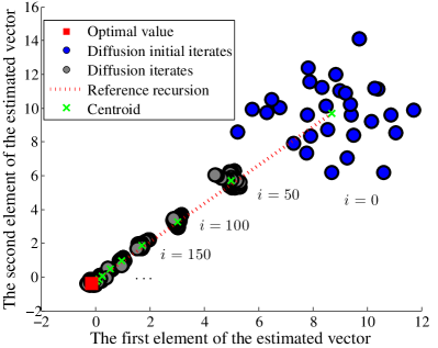
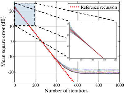
Figure 4: The evolution and learning curves of various quantities in a diffusion LMS adaptive network (best viewed in color), where $M=2$, and the regressors are spatially and temporally white, and isotropic across agents. (a) The evolution of the iterates $\{\bm{w}_{k,i}\}$ at all agents, the centroid $\bm{w}_{c,i}$, and the reference recursion $\bar{w}_{c,i}$ on the two-dimensional solution space; the horizontal axis and vertical axis are the first and second elements of $\bm{w}_{k,i}$, respectively. The clusters of $\{\bm{w}_{k,i}\}$ are plotted every $50$ iterations. (b) The MSE learning curves, averaged over $1000$ trials, for the iterates $\{\bm{w}_{k,i}\}$ at all agents, and the reference recursion $\bar{w}_{c,i}$. The zoom-in region shows the learning curves for different agents, which quick shrink together in Phase I.

The result established in Theorem 5 is significant because it allows us to examine the learning behavior of $\mathbb{E}\|\tilde{\bm{w}}_{k,i}\|^{2}$. First, note that the bound (143) established in Theorem 5 is non-asymptotic; that is, it holds for any $i\geq 0$. Let $e_{1}(i)$, $e_{2}(i)$, $e_{3}(i)$ and $e_{4}$ denote the four terms in (143):

$$e_{1}(i) \triangleq 2\|u_{L,k}\otimes I_{M}\|^{2}\cdot\mathds{1}^{T}\Gamma_{e}^{i}\mathcal{W}_{e,0}$$ (144)

$$e_{2}(i) \triangleq 2\|\tilde{w}_{c,0}\|\cdot\|u_{L,k}\otimes I_{M}\|\cdot\sqrt{\mathds{1}^{T}\Gamma_{e}^{i}\mathcal{W}_{e,0}}$$ (145)

$$e_{3}(i) \triangleq\gamma_{c}^{i}\cdot O(\mu_{\max}^{\frac{1}{2}})$$ (146)

$$e_{4} \triangleq O(\mu_{\max})$$ (147)

Then, inequality (143) can be rewritten as

$$\| \tilde{w}_{c,i}\|^{2}\!-\![e_{1}(i)+e_{2}(i)+e_{3}(i)+e_{4}]$$

$$\leq\mathbb{E}\|\tilde{\bm{w}}_{k,i}\|^{2}\leq\|\tilde{w}_{c,i}\|^{2}\!+\![e_{1}(i)\!+\!e_{2}(i)\!+\!e_{3}(i)\!+\!e_{4}]$$ (148)

for all $i\geq 0$. That is, the learning curve of $\mathbb{E}\|\tilde{\bm{w}}_{k,i}\|^{2}$ is a perturbed version of the learning curve of reference recursion $\|\tilde{w}_{c,i}\|^{2}$, where the perturbation consists of four parts: $e_{1}(i)$, $e_{2}(i)$, $e_{3}(i)$ and $e_{4}$. We now examine the non-asymptotic convergence rates of these four perturbation terms relative to that of the reference term $\|\tilde{w}_{c,i}\|^{2}$ to show how the learning behavior of $\mathbb{E}\|\tilde{\bm{w}}_{k,i}\|^{2}$ can be approximated by $\|\tilde{w}_{c,i}\|^{2}$. From their definitions in (144)–(145), we note that $e_{1}(i)$ and $e_{2}(i)$ converge to zero at the non-asymptotic rates of $\rho(\Gamma_{e})$ and $[\rho(\Gamma_{e})]^{\frac{1}{2}}$ over $i\geq 0$. According to (129), we have $\rho(\Gamma_{e})=|\lambda_{2}(A)|$, the magnitude of the second largest eigenvalue of $A$. Let $r_{e_{1}}$ and $r_{e_{2}}$ denote the convergence rates of $e_{1}(i)$ and $e_{2}(i)$. We have

$$r_{e_{1}}=|\lambda_{2}(A)|,\quad r_{e_{2}}=|\lambda_{2}(A)|^{\frac{1}{2}}$$ (149)

By Assumption 1 and (13), the value of $|\lambda_{2}(A)|$ is strictly less than one, and is determined by the network connectivity and the design of the combination matrix; it is also independent of the step-size parameter $\mu_{\max}$. For this reason, the terms $e_{1}(i)$ and $e_{2}(i)$ converge to zero at rates that are determined by the network and are independent of $\mu_{\max}$. Furthermore, the term $e_{3}(i)$ is always small, i.e., $O(\mu_{\max}^{\frac{1}{2}})$, for all $i\geq 0$, and converges to zero as $i\rightarrow\infty$. The last term $e_{4}$ is also small, namely, $O(\mu_{\max})$. On the other hand, as revealed by Theorem 2 and (123), the non-asymptotic convergence rate of the term $\|\tilde{w}_{c,i}\|^{2}$ in (148) is bounded by

$$1-2\mu_{\max}\|p\|_{1}\lambda_{U}\leq r_{\mathrm{Ref}}\leq\gamma_{c}^{2}=1-2\mu_{\max}\lambda_{L}+o(\mu_{\max})$$ (150)

Therefore, as long as $\mu_{\max}$ is small enough so that

$$|\lambda_{2}(A)|<|\lambda_{2}(A)|^{\frac{1}{2}}<1-2\mu_{\max}\|p\|_{1}\lambda_{U}$$ (151)

which is equivalent to requiring

$$\mu_{\max}<\frac{1-|\lambda_{2}(A)|^{\frac{1}{2}}}{2\|p\|_{1}\lambda_{U}}$$ (152)

we have the following relation regarding the non-asymptotic rates of $e_{1}(i)$, $e_{2}(i)$ and $\|\tilde{w}_{c,i}\|^{2}$:

$$r_{e_{1}}<r_{e_{2}}<r_{\mathrm{Ref}}$$ (153)

This means that, for sufficiently small $\mu_{\max}$ satisfying (152), $e_{1}(i)$ and $e_{2}(i)$ converge faster than $\|\tilde{w}_{c,i}\|^{2}$. For this reason, the perturbation terms $e_{1}(i)$ and $e_{2}(i)$ in (148) die out earlier than $\|\tilde{w}_{c,i}\|^{2}$. When they are negligible compared to $\|\tilde{w}_{c,i}\|^{2}$, we reach the end of Transient Phase I. Then, in Transient Phase II, we have

$$\|\tilde{w}_{c,i}\|^{2}\!-\![e_{3}(i)+e_{4}]\leq\mathbb{E}\|\tilde{\bm{w}}_{k,i}\|^{2}\leq\|\tilde{w}_{c,i}\|^{2}+[e_{3}(i)+e_{4}]$$ (154)

By (146) and (147), the above inequality (154) is equivalent to the following relation:

$$\mathbb{E}\|\tilde{\bm{w}}_{k,i}\|^{2}=\|\tilde{w}_{c,i}\|^{2}+O(\mu_{\max}^{\frac{1}{2}})\cdot\gamma_{c}^{i}+O(\mu_{\max})$$ (155)

This means that $\mathbb{E}\|\tilde{\bm{w}}_{k,i}\|^{2}$ is close to $\|\tilde{w}_{c,i}\|^{2}$ in Transient Phase II, and the convergence rate of $\mathbb{E}\|\tilde{\bm{w}}_{k,i}\|^{2}$ is the same as that of $\|\tilde{w}_{c,i}\|^{2}$. Furthermore, in the later stage of Transient Phase II, the convergence rate of $\mathbb{E}\|\tilde{\bm{w}}_{k,i}\|^{2}$ would be close to the asymptotic rate of $\|\tilde{w}_{c,i}\|^{2}$ given by (124). Afterwards, as $i\rightarrow\infty$, both $\|\tilde{w}_{c,i}\|^{2}$ and $O(\mu_{\max}^{\frac{1}{2}})\cdot\gamma_{c}^{i}$ converge to zero and the only term remaining will be $e_{4}=O(\mu_{\max})$, which contributes to the steady-state MSE. More specifically, taking the $\limsup$ of both sides of (143) leads to

$$\limsup_{i\rightarrow\infty}\mathbb{E}\|\tilde{\bm{w}}_{k,i}\|^{2} =\limsup_{i\rightarrow\infty}\big{|}\mathbb{E}\|\tilde{\bm{w}}_{k,i}\|^{2}-\|\tilde{w}_{c,i}\|^{2}\big{|}$$

$$\leq O(\mu_{\max})$$ (156)

We will go a step further and evaluate this steady-state MSE in closed-form for small step-sizes in Part II [44]. Therefore, $\bm{w}_{k,i}$ converges to $w^{o}$ with a small steady-state MSE that is on the order of $O(\mu_{\max})$. And the steady-state MSE can be made arbitrarily small for small step-sizes.

In view of this discussion, we now recognize that the results established in Theorems 1–4 reveal the evolution of the three components, $\tilde{w}_{c,i}$, $\check{\bm{w}}_{c,i}$ and $\bm{w}_{e,i}$ in (84) during three distinct phases of the learning process. From (134), the centroid $\bm{w}_{c,i}$ of the distributed algorithm (1)–(3) stays close to $\bar{w}_{c,i}$ over the entire time for sufficiently small step-sizes since the mean-square error $\mathbb{E}\|\bm{w}_{c,i}-\bar{w}_{c,i}\|^{2}=\mathbb{E}P[\check{\bm{w}}_{c,i}]$ is always of the order of $O(\mu_{\max})$. However, $\mathcal{W}_{e,0}=\mathbb{E}P[\bm{w}_{e,i}]$ in (135) is not necessarily small at the beginning. This is because, as we pointed out in (80) and Fig. 3, $\bm{w}_{e,i}$ characterizes the deviation of the agents from their centroid. If the agents are initialized at different values, then $\mathbb{E}P[\bm{w}_{e,0}]\neq 0$, and it takes some time for $\mathbb{E}P[\bm{w}_{e,i}]$ to decay to a small value of $O(\mu_{\max}^{2})$. By (135), the rate at which $\mathbb{E}P[\bm{w}_{e,i}]$ decays is $\rho(\Gamma_{e})=|\lambda_{2}(A)|$. On the other hand, recall from Theorems 2–3 that the error of the reference recursion, $\tilde{w}_{c,i}$ converges at a rate between $1-2\mu_{\max}\|p\|_{1}\lambda_{U}$ and $r_{c}^{2}=1-2\mu_{\max}\lambda_{L}+o(\lambda_{\max})$ at beginning and then $[\rho(I_{M}-\mu_{\max}H_{c})]^{2}$ later on, which is slower than the convergence rate of $\mathbb{E}P[\bm{w}_{e,i}]$ for small step-size $\mu_{\max}$. Now, returning to relation (84):

$$\tilde{\bm{w}}_{k,i} =\tilde{w}_{c,i}-\check{\bm{w}}_{c,i}-(u_{L,k}\otimes I_{M})\bm{w}_{e,i}$$ (157)

this means that during the initial stage of adaptation, the third term in (157) decays to $O(\mu_{\max}^{2})$ at a faster rate than the first term, although $\tilde{w}_{c,i}$ will eventually converge to zero. Recalling from (80) and Fig. 3 that $\bm{w}_{e,i}$ characterizes the deviation of the agents from their centroid, the decay of $\bm{w}_{e,i}$ implies that the agents are coordinating with each other so that their estimates $\bm{w}_{k,i}$ are close to the same $\bm{w}_{c,i}$ — we call this stage Transient Phase I. Moreover, as we just pointed out, the term $\mathbb{E}P[\check{\bm{w}}_{c,i}]$ is $O(\mu_{\max})$ over the entire time domain so that the second term in (157) is always small. This also means that the centroid of the cluster in Fig. 3, i.e., $\bm{w}_{c,i}$, is always close to the reference recursion $\bar{w}_{c,i}$ since $\check{\bm{w}}_{c,i}=\bm{w}_{c,i}-\bar{w}_{c,i}$ is always small. Now that $\mathbb{E}\|\check{\bm{w}}_{c,i}\|^{2}$ is $O(\mu_{\max})$ and $\mathbb{E}P[\bm{w}_{e,i}]$ is $O(\mu_{\max}^{2})$, the error $\tilde{\bm{w}}_{k,i}$ at each agent $k$ is mainly dominated by the first term, $\tilde{w}_{c,i}$, in (157), and the estimates $\{\bm{w}_{k,i}\}$ at different agents converge together at the same rate as the reference recursion, given by (124), to steady-state — we call this stage Transient Phase II. Furthermore, if $\mathcal{W}_{e,0}=0$, i.e., the iterates $\bm{w}_{k,i}$ are initialized at the same value (e.g., zero vector), then (135) shows that $\mathbb{E}P[\bm{w}_{e,i}]$ is $O(\mu_{\max}^{2})$ over the entire time domain so that the learning dynamics start at Transient Phase II directly. Finally, all agents reach the third phase, steady-state, where $\tilde{w}_{c,i}\rightarrow 0$ and $\tilde{\bm{w}}_{k,i}$ is dominated by the second and third terms in (157) so that $\mathbb{E}\|\tilde{\bm{w}}_{k,i}\|^{2}$ becomes $O(\mu_{\max})$. We summarize the above results in Table III and illustrate the evolution of the quantities in the simulated example in Fig. 4. We observe from Fig. 4 that the radius of the cluster shrinks quickly at the early stage of the transient phase, and then converges towards the optimal solution.

VII Conclusion

In this work, we studied the learning behavior of adaptive networks under fairly general conditions. We showed that, in the constant and small step-size regime, a typical learning curve of each agent exhibits three phases: Transient Phase I, Transient Phase II, and Steady-state Phase. A key observation is that, the second and third phases approach the performance of a centralized strategy. Furthermore, we showed that the right eigenvector of the combination matrix corresponding to the eigenvalue at one influences the limit point, the convergence rate, and the steady-state mean-square-error (MSE) performance of the distributed optimization and learning strategies in a critical way. Analytical expressions that illustrate these effects were derived. Various implications were discussed and illustrative examples were also considered.

Appendix A Properties of the Energy Operators

In this appendix, we state lemmas on properties of the operators $P_{M_{0}}[\cdot]$ and $\bar{P}_{M_{0}}[\cdot]$. We begin with some basic properties.

Lemma 5 (Basic properties)

Consider $N\times 1$ block vectors $x=\mathrm{col}\{x_{1},\ldots,x_{N}\}$ and $y=\mathrm{col}\{y_{1},\ldots,y_{N}\}$ with $M\times 1$ entries $\{x_{k},y_{k}\}$. Consider also the $K\times N$ block matrix $X$ with blocks of size $M\times M$. Then, the operators $P[\cdot]$ and $\bar{P}[\cdot]$ satisfy the following properties:

1. (Nonnegativity): $P[x]\succeq 0$, $\bar{P}[X]\succeq 0$.

2. (Scaling): For any scalar $a\in\mathbb{C}$, we have $P[ax]=|a|^{2}P[x]$ and $\bar{P}[aX]=|a|\cdot\bar{P}[X]$.

3. (Convexity): suppose $x^{(1)},\ldots,x^{(K)}$ are $N\times 1$ block vectors formed in the same manner as $x$, $X^{(1)},\ldots,X^{(K)}$ are $K\times N$ block matrices formed in the same manner as $X$, and let $a_{1},\ldots,a_{K}$ be non-negative real scalars that add up to one. Then,

   $$P[a_{1}x^{(1)} +\cdots+a_{K}x^{(K)}]$$

   $$\preceq a_{1}P[x^{(1)}]+\cdots+a_{K}P[x^{(K)}]$$ (158)

   $$\bar{P}[a_{1}X^{(1)} +\cdots+a_{K}X^{(K)}]$$

   $$\preceq a_{1}\bar{P}[X^{(1)}]+\cdots+a_{K}\bar{P}[X^{(K)}]$$ (159)

4. (Additivity): Suppose $\bm{x}=\mathrm{col}\{\bm{x}_{1},\ldots,\bm{x}_{N}\}$ and $\bm{y}=\mathrm{col}\{\bm{y}_{1},\ldots,\bm{y}_{N}\}$ are $N\times 1$ block random vectors that satisfy $\mathbb{E}\bm{x}_{k}^{*}\bm{y}_{k}=0$ for $k=1,\ldots,N$, where $*$ denotes complex conjugate transposition. Then,

   $$\mathbb{E}P[\bm{x}+\bm{y}]=\mathbb{E}P[\bm{x}]+\mathbb{E}P[\bm{y}]$$ (160)

5. (Triangular inequality): Suppose $X$ and $Y$ are two $K\times N$ block matrices of same block size $M$. Then,

   $$\bar{P}[X+Y]\preceq\bar{P}[X]+\bar{P}[Y]$$ (161)

6. (Submultiplicity): Suppose $X$ and $Z$ are $K\times N$ and $N\times L$ block matrices of the same block size $M$, respectively. Then,

   $$\bar{P}[XZ]\preceq\bar{P}[X]\bar{P}[Z]$$ (162)

7. (Kronecker structure): Suppose $X\in\mathbb{C}^{K\times N}$, $a\in\mathbb{C}^{N}$ and $b\in\mathbb{C}^{M}$. Then,

   $$\bar{P}[X\otimes I_{M}] =\bar{P}_{1}[X]$$ (163)

   $$P[a\otimes b] =\|b\|^{2}\cdot P_{1}[a]$$ (164)

   where by definition, $\bar{P}_{1}[\cdot]$ and $P_{1}[\cdot]$ denote the operators that work on the scalar entries of their arguments. When $X$ consists of nonnegative entries, relation (163) becomes

   $$\bar{P}[X\otimes I_{M}] =X$$ (165)

8. (Relation to norms): The $\infty-$norm of $P[x]$ is the squared block maximum norm of $x$:

   $$\|P[x]\|_{\infty}=\|x\|_{b,\infty}^{2}\triangleq\big{(}\max_{1\leq k\leq N}\|x_{k}\|\big{)}^{2}$$ (166)

   Moreover, the sum of the entries in $P[x]$ is the squared Euclidean norm of $x$:

   $$\mathds{1}^{T}P[x]=\|x\|^{2}=\sum_{k=1}^{N}\|x_{k}\|^{2}$$ (167)

9. (Inequality preservation): Suppose vectors $x$, $y$ and matrices $F$, $G$ have nonnegative entries, then $x\preceq y$ implies $Fx\preceq Fy$, and $F\preceq G$ implies $Fx\preceq Gx$.

10. (Upper bounds): It holds that

    $$\bar{P}[X] \preceq\|\bar{P}[X]\|_{1}\cdot\mathds{1}\mathds{1}^{T}$$ (168)

    $$\bar{P}[X] \preceq\|\bar{P}[X]\|_{\infty}\cdot\mathds{1}\mathds{1}^{T}$$ (169)

    where $\|\cdot\|_{\infty}$ denotes the $\infty-$induced norm of a matrix (maximum absolute row sum).

Proof:

See Appendix C. ∎

More importantly, the following variance relations hold for the energy and norm operators. These relations show how error variances propagate after a certain operator is applied to a random vector.

Lemma 6 (Variance relations)

Consider $N\times 1$ block vectors $x=\mathrm{col}\{x_{1},\ldots,x_{N}\}$ and $y=\mathrm{col}\{y_{1},\ldots,y_{N}\}$ with $M\times 1$ entries $\{x_{k},y_{k}\}$. The following variance relations are satisfied by the energy vector operator $P[\cdot]$:

1. (Linear transformation): Given a $K\times N$ block matrix $Q$ with the size of each block being $M\times M$, $Qx$ defines a linear operator on $x$ and its energy satisfies

   $$P[Qx] \preceq\|\bar{P}[Q]\|_{\infty}\cdot\bar{P}[Q]\;P[x]$$ (170)

   $$\preceq\|\bar{P}[Q]\|_{\infty}^{2}\cdot\mathds{1}\mathds{1}^{T}\cdot P[x]$$ (171)

   As a special case, for a left-stochastic $N\times N$ matrix $A$, we have

   $$P[(A^{T}\otimes I_{M})x]\preceq A^{T}P[x]$$ (172)

2. (Update operation): The global update vector defined by (95) satisfies the following variance relation:

   $$P[s(x)-s(y)]\preceq\lambda_{U}^{2}P[x-y]$$ (173)

3. (Centralized operation): The centralized operator $T_{c}(x)$ defined by (109) satisfies the following variance relations:

   $$P[T_{c}(x)-T_{c}(y)] \preceq\gamma_{c}^{2}\cdot P[x-y]$$ (174)

   $$P[T_{c}(x)-T_{c}(y)] \succeq(1-2\mu_{\max}\|p\|_{1}\lambda_{U})\cdot P[x-y]$$ (175)

   where

   $$\gamma_{c}\triangleq 1-\mu_{\max}\lambda_{L}+\frac{1}{2}\mu_{\max}^{2}\|p\|_{1}^{2}\lambda_{U}^{2}$$ (176)

   Moreover, it follows from (26) that

   $$\gamma_{c} \geq 1-\mu_{\max}\lambda_{L}+\frac{1}{2}\mu_{\max}^{2}\lambda_{L}^{2}$$

   $$=(1-\frac{1}{2}\mu_{\max}\lambda_{L})^{2}+\frac{1}{4}\mu_{\max}^{2}\lambda_{L}^{2}>0$$ (177)

4. (Stable Jordan operation): Suppose $D_{L}$ is an $L\times L$ Jordan matrix of the following block form:

   $$D_{L} \triangleq\mathrm{diag}\{D_{L,2},\ldots,D_{L,n_{0}}\}$$ (178)

   where the $n$th $L_{n}\times L_{n}$ Jordan block is defined as (note that $L=L_{2}+\cdots+L_{n_{0}}$)

   $$D_{L,n} \triangleq\begin{bmatrix}d_{n}&1&&\\ &\ddots&\ddots&\\ &&\ddots&1\\ &&&d_{n}\end{bmatrix}$$ (179)

   We further assume $D_{L}$ to be stable with $0\leq|d_{n_{0}}|\leq\cdots\leq|d_{2}|<1$. Then, for any $L\times 1$ vectors $x^{\prime}$ and $y^{\prime}$, we have

   $$P_{1}[D_{L}x^{\prime}+y^{\prime}]\preceq\Gamma_{e}\cdot P_{1}[x^{\prime}]+\frac{2}{1-|d_{2}|}\cdot P_{1}[y^{\prime}]$$ (180)

   where $\Gamma_{e}$ is the $L\times L$ matrix defined as

   $$\Gamma_{e} \triangleq\begin{bmatrix}|d_{2}|&\frac{2}{1-|d_{2}|}&&\\ &\ddots&\ddots&\\ &&\ddots&\frac{2}{1-|d_{2}|}\\ &&&|d_{2}|\end{bmatrix}$$ (181)

5. (Stable Kronecker Jordan operator): Suppose $\mathcal{D}_{L}=D_{L}\otimes I_{M}$, where $D_{L}$ is the $L\times L$ Jordan matrix defined in (178)–(179). Then, for any $LM\times 1$ vectors $x_{e}$ and $y_{e}$, we have

   $$P[\mathcal{D}_{L}x_{e}+y_{e}]\preceq\Gamma_{e}\cdot P[x_{e}]+\frac{2}{1-|d_{2}|}\cdot P[y_{e}]$$ (182)

Proof:

See Appendix D. ∎

Appendix B Proof of Lemma 1

First, we establish that conditions (27) and (28) imply (24) and (25), respectively. Using the mean-value theorem[49, p.6], we have for any $x,y\in\mathcal{S}$:

$$\left\|s_{k}(x)-s_{k}(y)\right\| =\left\|\int_{0}^{1}\nabla_{w^{T}}s_{k}(y+t(x-y))dt\cdot(x-y)\right\|$$

$$\leq\int_{0}^{1}\left\|\nabla_{w^{T}}s_{k}(y+t(x-y))\right\|dt\cdot\|x-y\|$$

$$\leq\lambda_{U}\cdot\|x-y\|$$ (183)

where we used the fact that $y+t(x-y)=tx+(1-t)y\in\mathcal{S}$ given $x,y\in\mathcal{S}$ and $0\leq t\leq 1$. Likewise, we have

$$(x-y)^{T}\cdot\sum_{k=1}^{N}p_{k}[s_{k}(x)-s_{k}(y)]$$

$$=(x-y)^{T}\cdot\sum_{k=1}^{N}p_{k}\int_{0}^{1}\nabla_{w^{T}}s_{k}(y+t(x-y))dt\cdot(x-y)$$

$$=(x-y)^{T}\cdot\int_{0}^{1}\sum_{k=1}^{N}p_{k}\nabla_{w^{T}}s_{k}(y+t(x-y))dt\cdot(x-y)$$

$$\overset{\eqref{Equ:Lemma:EquivCondUpdateVec:Hc_def}}{=}(x-y)^{T}\cdot H_{c}(y+t(x-y))\cdot(x-y)$$

$$=(x\!-\!y)^{T}\!\cdot\!\frac{H_{c}(y+t(x-y))+H_{c}^{T}(y+t(x-y))}{2}\!\cdot\!(x\!-\!y)$$

$$\geq\lambda_{L}\cdot\|x-y\|^{2}$$ (184)

Next, we establish the reverse direction that conditions (24) and (25) imply (27) and (28). Choosing $x=w+t\cdot\delta w$ and $y=w$ in (24) for any $\delta w\neq 0$ and any small positive $t$, we get

$$\| s_{k}(w+t\cdot\delta w)-s_{k}(w)\|\leq t\cdot\lambda_{U}\cdot\|\delta w\|$$

$$\Rightarrow\quad\lim_{t\rightarrow 0^{+}}\left\|\frac{s_{k}(w+t\cdot\delta w)-s_{k}(w)}{t}\right\|\leq\lambda_{U}\cdot\|\delta w\|$$

$$\Rightarrow\quad\left\|\lim_{t\rightarrow 0^{+}}\frac{s_{k}(w+t\cdot\delta w)-s_{k}(w)}{t}\right\|\leq\lambda_{U}\cdot\|\delta w\|$$

$$\Rightarrow\quad\left\|\nabla_{w^{T}}s_{k}(w)\delta w\right\|\leq\lambda_{U}\cdot\|\delta w\|$$

$$\Rightarrow\quad\|\nabla_{w^{T}}s_{k}(w)\|\triangleq\sup_{\delta w\neq 0}\frac{\left\|\nabla_{w^{T}}s_{k}(w)\delta w\right\|}{\|\delta w\|}\leq\lambda_{U}$$ (185)

Likewise, choosing $x=w+t\cdot\delta w$ and $y=w$ in (25) for any $\delta w\neq 0$ and any small positive $t$, we obtain

$$t\cdot\delta w^{T} \cdot\sum_{k=1}^{N}p_{k}[s_{k}(w+t\cdot\delta w)-s_{k}(w)]\geq t^{2}\cdot\lambda_{L}\cdot\|\delta w\|^{2}$$

$$\Rightarrow\quad\delta w^{T}\cdot\sum_{k=1}^{N}p_{k}\left(\lim_{t\rightarrow 0^{+}}\frac{s_{k}(w+t\cdot\delta w)-s_{k}(w)}{t}\right)$$

$$\qquad\qquad\geq\lambda_{L}\cdot\|\delta w\|^{2}$$

$$\Rightarrow\quad\delta w^{T}\cdot\sum_{k=1}^{N}p_{k}\nabla_{w^{T}}s_{k}(w)\cdot\delta w\geq\lambda_{L}\cdot\|\delta w\|^{2}$$

$$\Rightarrow\quad\delta w^{T}H_{c}(w)\delta w\geq\lambda_{L}\cdot\|\delta w\|^{2}$$

$$\Rightarrow\quad\delta w^{T}\frac{H_{c}(w)+H_{c}^{T}(w)}{2}\delta w\geq\lambda_{L}\cdot\|\delta w\|^{2}$$

$$\Rightarrow\quad\frac{H_{c}(w)+H_{c}^{T}(w)}{2}\geq\lambda_{L}\cdot I_{M}$$ (186)

Appendix C Proof of Lemma 5

Properties 1-2 are straightforward from the definitions of $P[\cdot]$ and $\bar{P}[\cdot]$. Property 4 was proved in [20]. We establish the remaining properties.

(Property 3: Convexity) The convexity of $P[\cdot]$ has already been proven in [20]. We now establish the convexity of the operator $\bar{P}[\cdot]$. Let $X_{qn}^{(k)}$ denote the $(q,n)-$th $M\times M$ block of the matrix $X^{(k)}$, where $q=1,\ldots,K$ and $n=1,\ldots,N$. Then,

$$\bar{P} \left[\sum_{k=1}^{K}a_{k}X^{(k)}\right]$$

$$\preceq\begin{bmatrix}\sum_{k=1}^{K}a_{k}\left\|X_{11}^{(k)}\right\|&\cdots&\sum_{k=1}^{K}a_{k}\left\|X_{1N}^{(k)}\right\|\\ \vdots&&\vdots\\ \sum_{k=1}^{K}a_{k}\left\|X_{K1}^{(k)}\right\|&\cdots&\sum_{k=1}^{K}a_{k}\left\|X_{KN}^{(k)}\right\|\end{bmatrix}$$

$$=\sum_{k=1}^{K}a_{k}\bar{P}[X^{(k)}]$$ (187)

(Property 5: Triangular inequality) Let $X_{qn}$ and $Y_{qn}$ denote the $(q,n)-$th $M\times M$ blocks of the matrices $X$ and $Y$, respectively, where $q=1,\ldots,K$ and $n=1,\ldots,N$. Then, by the triangular inequality of the matrix norm $\|\cdot\|$, we have

$$\bar{P}\left[X+Y\right] \preceq\begin{bmatrix}\left\|X_{11}\right\|+\left\|Y_{11}\right\|&\cdots&\left\|X_{1N}\right\|+\left\|Y_{1N}\right\|\\ \vdots&&\vdots\\ \left\|X_{K1}\right\|+\left\|Y_{K1}\right\|&\cdots&\left\|X_{KN}\right\|+\left\|Y_{KN}\right\|\end{bmatrix}$$

$$=\bar{P}[X]+\bar{P}[Y]$$ (188)

(Property 6: Submultiplicity) Let $X_{kn}$ and $Z_{nl}$ be the $(k,n)-$th and $(n,l)-$th $M\times M$ blocks of $X$ and $Z$, respectively. Then, the $(k,l)-$th $M\times M$ block of the matrix product $XZ$, denoted by $[XZ]_{k,l}$, is

$$[XZ]_{k,l}=\sum_{n=1}^{N}X_{kn}Z_{nl}$$ (189)

Therefore, the $(k,l)-$th entry of the matrix $\bar{P}[XZ]$ can be bounded as

$$\big{[}\bar{P}[XZ]\big{]}_{k,l} =\left\|\sum_{n=1}^{N}X_{kn}Z_{nl}\right\|\leq\sum_{n=1}^{N}\left\|X_{kn}\right\|\cdot\left\|Z_{nl}\right\|$$ (190)

Note that $\|X_{kn}\|$ and $\|Z_{nl}\|$ are the $(k,n)-$th and $(n,l)-$th entries of the matrices $\bar{P}[X]$ and $\bar{P}[Z]$, respectively. The right-hand side of the above inequality is therefore the $(k,l)-$th entry of the matrix product $\bar{P}[X]\bar{P}[Z]$. Therefore, we obtain

$$\bar{P}[XZ]\preceq\bar{P}[X]\bar{P}[Z]$$ (191)

(Property 7: Kronecker structure) For (163), we note that the $(k,n)-$th $M\times M$ block of $X\otimes I_{M}$ is $x_{kn}I_{M}$. Therefore, by the definition of $\bar{P}[\cdot]$, we have

$$\bar{P}[X\otimes I_{M}] =\begin{bmatrix}|x_{11}|&\cdots&|x_{1N}|\\ \vdots&&\\ |x_{K1}|&\cdots&|x_{KN}|\end{bmatrix}=\bar{P}_{1}[X]$$ (192)

In the special case when $X$ consists of nonnegative entries, $\bar{P}_{1}[X]=X$, and we recover (165). To prove (164), we let $a=\mathrm{col}\{a_{1},\ldots,a_{N}\}$ and $b=\mathrm{col}\{b_{1},\ldots,b_{M}\}$. Then, by the definitin of $P[\cdot]$, we have

$$P[a\otimes b]=\mathrm{col}\{|a_{1}|^{2}\cdot\|b\|^{2},\ldots,|a_{N}|^{2}\cdot\|b\|^{2}\}=\|b\|^{2}\cdot P_{1}[a]$$ (193)

(Property 8: Relation to norms) Relations (166) and (167) are straightforward and follow from the definition.

(Property 9: Inequality preservation) The proof that $x\preceq y$ implies $Fx\preceq Fy$ can be found in [20]. We now prove that $F\preceq G$ implies $Fx\preceq Gx$. This can be proved by showig that $(G-F)x\succeq 0$, which is true because all entries of $G-F$ and $x$ are nonnegative due to $F\preceq G$ and $x\succeq 0$.

(Property 10: Upper bounds) By the definition of $\bar{P}[X]$ in (117), we get

$$\bar{P}[X] \preceq\left(\max_{l,k}\|X_{lk}\|\right)\cdot\mathds{1}\mathds{1}^{T}$$

$$\preceq\max_{l}\left(\sum_{k=1}^{N}\|X_{lk}\|\right)\cdot\mathds{1}\mathds{1}^{T}$$

$$=\|\bar{P}[X]\|_{\infty}\cdot\mathds{1}\mathds{1}^{T}$$ (194)

Likewise, we can establish that $\bar{P}[X]\preceq\|\bar{P}[X]\|_{1}\cdot\mathds{1}\mathds{1}^{T}$.

Appendix D Proof of Lemma 6

(Property 1: Linear transformation) Let $Q_{kn}$ be the $(k,n)$-th $M\times M$ block of $Q$. Then

$$P[Qx]=\mathrm{col}\left\{\left\|\sum_{n=1}^{N}Q_{1n}x_{n}\right\|^{2},\ldots,\left\|\sum_{n=1}^{N}Q_{Kn}x_{n}\right\|^{2}\right\}$$ (195)

Using the convexity of $\|\cdot\|^{2}$, we have the following bound on each $n$-th entry:

$$\bigg{\|} \sum_{n=1}^{N}Q_{kn}x_{n}\bigg{\|}^{2}$$

$$\overset{(a)}{=}\left[\sum_{n=1}^{N}\|Q_{kn}\|\right]^{2}\cdot\left\|\sum_{n=1}^{N}\frac{\|Q_{kn}\|}{\sum_{l=1}^{N}\|Q_{kl}\|}\cdot\frac{Q_{kn}}{\|Q_{kn}\|}x_{n}\right\|^{2}$$

$$\overset{(b)}{\leq}\left[\sum_{n=1}^{N}\|Q_{kn}\|\right]^{2}\cdot\sum_{n=1}^{N}\frac{\|Q_{kn}\|}{\sum_{l=1}^{N}\|Q_{kl}\|}\cdot\frac{\|Q_{kn}\|^{2}}{\|Q_{kn}\|^{2}}\|x_{n}\|^{2}$$

$$=\left[\sum_{n=1}^{N}\|Q_{kn}\|\right]\cdot\sum_{n=1}^{N}\|Q_{kn}\|\cdot\|x_{n}\|^{2}$$

$$\leq\max_{k}\left[\sum_{n=1}^{N}\|Q_{kn}\|\right]\cdot\sum_{n=1}^{N}\|Q_{kn}\|\cdot\|x_{n}\|^{2}$$

$$=\|\bar{P}[Q]\|_{\infty}\cdot\sum_{n=1}^{N}\|Q_{kn}\|\cdot\|x_{n}\|^{2}$$ (196)

where in step (b) we applied Jensen’s inequlity to $\|\cdot\|^{2}$. Note that if some $\|Q_{kn}\|$ in step (a) is zero, we eliminate the corresponding term from the sum and it can be verified that the final result still holds. Substituting into (195), we establish (170). The special case (172) can be obtained by using $\bar{P}[A^{T}\otimes I_{M}]=A^{T}$ and that $\|A^{T}\|_{\infty}=1$ (left-stochastic) in (170). Finally, the upper bound (171) can be proved by applying (169) to $\bar{P}[Q]$.

(Property 2: Update operation) By the definition of $P[\cdot]$ and the Lipschitz Assumption 3, we have

$$P [s(x)-s(y)]$$

$$=\mathrm{col}\{\|s_{1}(x_{1})-s_{1}(y_{1})\|^{2},\ldots\|s_{N}(x_{N})-s_{N}(y_{N})\|^{2}\}$$

$$\preceq\mathrm{col}\{\lambda_{U}^{2}\cdot\|x_{1}-y_{1}\|^{2},\ldots\lambda_{U}^{2}\cdot\|x_{N}-y_{N}\|^{2}\}$$

$$=\lambda_{U}^{2}\cdot P[x-y]$$ (197)

(Property 3: Centralized opertion) Since $T_{c}:\mathbb{R}^{M}\rightarrow\mathbb{R}^{M}$, the output of $P[T_{c}(x)-T_{c}(y)]$ becomes a scalar. From the definition, we get

$$P \left[T_{c}(x)-T_{c}(y)\right]$$

$$=\left\|x-y-\mu_{\max}\cdot(p^{T}\otimes I_{M})\left[s(\mathds{1}\otimes x)-s(\mathds{1}\otimes y)\right]\right\|^{2}$$

$$=\big{\|}x-y-\mu_{\max}\cdot\sum_{k=1}^{N}p_{k}\left[s_{k}(x)-s_{k}(y)\right]\big{\|}^{2}$$

$$=\left\|x-y\right\|^{2}-2\mu_{\max}\cdot(x-y)^{T}\sum_{k=1}^{N}p_{k}\left[s_{k}(x)-s_{k}(y)\right]$$

$$\quad+\mu_{\max}^{2}\left\|(p^{T}\otimes I_{M})\left[s(\mathds{1}\otimes x)-s(\mathds{1}\otimes y)\right]\right\|^{2}$$

$$=\left\|x-y\right\|^{2}-2\mu_{\max}\cdot(x-y)^{T}\sum_{k=1}^{N}p_{k}\left[s_{k}(x)-s_{k}(y)\right]$$

$$\quad+\mu_{\max}^{2}P\left[(p^{T}\otimes I_{M})\left[s(\mathds{1}\otimes x)-s(\mathds{1}\otimes y)\right]\right]$$ (198)

We first prove the upper bound (174) as follows:

$$P \left[T_{c}(x)-T_{c}(y)\right]$$

$$=\big{\|}x-y-\mu_{\max}\cdot\sum_{k=1}^{N}p_{k}[s_{k}(x)-s_{k}(y)]\big{\|}^{2}$$

$$=\|x-y\|^{2}-2\mu_{\max}\cdot(x-y)^{T}\sum_{k=1}^{N}p_{k}[s_{k}(x)-s_{k}(y)]$$

$$\quad+\mu_{\max}^{2}\cdot\big{\|}\sum_{k=1}^{N}p_{k}[s_{k}(x)-s_{k}(y)]\big{\|}^{2}$$

$$\overset{\eqref{Equ:Assumption:StrongMonotone}}{\leq}\|x-y\|^{2}-2\mu_{\max}\cdot\lambda_{L}\cdot\|x-y\|^{2}$$

$$\quad+\mu_{\max}^{2}\cdot\big{\|}\sum_{k=1}^{N}p_{k}[s_{k}(x)-s_{k}(y)]\big{\|}^{2}$$

$$\leq\|x-y\|^{2}-2\mu_{\max}\cdot\lambda_{L}\cdot\|x-y\|^{2}$$

$$\quad+\mu_{\max}^{2}\cdot\big{[}\sum_{k=1}^{N}p_{k}\|s_{k}(x)-s_{k}(y)\|\big{]}^{2}$$

$$\overset{\eqref{Equ:Assumption:Lipschitz}}{\leq}\|x-y\|^{2}-2\mu_{\max}\cdot\lambda_{L}\cdot\|x-y\|^{2}$$

$$\quad+\mu_{\max}^{2}\cdot\left[\sum_{k=1}^{N}p_{k}\cdot\lambda_{U}\cdot\|x-y\|\right]^{2}$$

$$=\|x-y\|^{2}-2\mu_{\max}\cdot\lambda_{L}\cdot\|x-y\|^{2}$$

$$\quad+\mu_{\max}^{2}\cdot\|p\|_{1}^{2}\lambda_{U}^{2}\cdot\|x-y\|^{2}$$

$$=(1-2\mu_{\max}\lambda_{L}+\mu_{\max}^{2}\lambda_{U}^{2}\|p\|_{1}^{2})\cdot\|x-y\|^{2}$$

$$\leq\left(1-\mu_{\max}\lambda_{L}+\frac{1}{2}\mu_{\max}^{2}\lambda_{U}^{2}\|p\|_{1}^{2}\right)^{2}\cdot\|x-y\|^{2}$$ (199)

where in the last step we used the relation $(1-x)\leq(1-\frac{1}{2}x)^{2}$.

Next, we prove the lower bound (175). From (198), we notice that the last term in (198) is always nonnegative so that

$$P \left[T_{c}(x)-T_{c}(y)\right]$$

$$\succeq\left\|x-y\right\|^{2}-2\mu_{\max}\cdot(x-y)^{T}\sum_{k=1}^{N}p_{k}\left[s_{k}(x)-s_{k}(y)\right]$$

$$\overset{(a)}{\succeq}\left\|x-y\right\|^{2}-2\mu_{\max}\cdot\|x-y\|\cdot\big{\|}\sum_{k=1}^{N}p_{k}\left[s_{k}(x)-s_{k}(y)\right]\big{\|}$$

$$\succeq\left\|x-y\right\|^{2}-2\mu_{\max}\cdot\|x-y\|\cdot\sum_{k=1}^{N}p_{k}\left\|s_{k}(x)-s_{k}(y)\right\|$$

$$\overset{(b)}{\succeq}\left\|x-y\right\|^{2}-2\mu_{\max}\cdot\|x-y\|\cdot\sum_{k=1}^{N}p_{k}\lambda_{U}\|x-y\|$$

$$=(1-2\mu_{\max}\lambda_{U}\|p\|_{1})\cdot\|x-y\|^{2}$$ (200)

where in step (a), we used the Cauchy-Schwartz inequality $x^{T}y\leq|x^{T}y|\leq\|x\|\cdot\|y\|$, and in step (b) we used (24).

(Property 4: Stable Jordan operator) First, we notice that matrix $D_{L,n}$ can be written as

$$D_{L,n}=d_{n}\cdot I_{L_{n}}+\Theta_{L_{n}}$$ (201)

where $\Theta_{L_{n}}$ is an $L_{n}\times L_{n}$ strictly upper triangular matrix of the following form:

$$\Theta_{L_{n}}\triangleq\begin{bmatrix}0&1&&\\ &\ddots&\ddots&\\ &&\ddots&1\\ &&&0\end{bmatrix}$$ (202)

Define the following matrices:

$$\Lambda_{L} \triangleq\mathrm{diag}\{d_{2}I_{L_{2}},\ldots,d_{n_{0}}I_{L_{n_{0}}}\}$$ (203)

$$\Theta_{L}^{\prime} \triangleq\mathrm{diag}\{\Theta_{L_{2}},\ldots,\Theta_{L_{n_{0}}}\}$$ (204)

Then, the original Jordan matrix $D_{L}$ can be expressed as

$$D_{L}=\Lambda_{L}+\Theta_{L}^{\prime}$$ (205)

so that

$$P_{1} [D_{L}x^{\prime}+y^{\prime}]$$

$$=P_{1}\left[\Lambda_{L}x^{\prime}+\Theta_{L}^{\prime}x^{\prime}+y^{\prime}\right]$$

$$=P_{1}\bigg{[}|d_{2}|\cdot\frac{1}{|d_{2}|}\Lambda_{L}x^{\prime}+\frac{1-|d_{2}|}{2}\cdot\frac{2}{1-|d_{2}|}\Theta_{L}^{\prime}x^{\prime}$$

$$\qquad+\frac{1-|d_{2}|}{2}\cdot\frac{2}{1-|d_{2}|}y^{\prime}\bigg{]}$$

$$\overset{(a)}{\preceq}|d_{2}|\cdot P_{1}\left[\frac{1}{|d_{2}|}\Lambda_{L}x^{\prime}\right]+\frac{1-|d_{2}|}{2}\cdot P_{1}\left[\frac{2}{1-|d_{2}|}\Theta_{L}^{\prime}x^{\prime}\right]$$

$$\quad+\frac{1-|d_{2}|}{2}\cdot P_{1}\left[\frac{2}{1-|d_{2}|}y^{\prime}\right]$$

$$\overset{(b)}{=}\frac{1}{|d_{2}|}\!\cdot\!P_{1}\left[\Lambda_{L}x^{\prime}\right]\!+\!\frac{2}{1-|d_{2}|}\!\cdot\!P_{1}\left[\Theta_{L}^{\prime}x^{\prime}\right]\!+\!\frac{2}{1-|d_{2}|}\!\cdot\!P_{1}\left[y^{\prime}\right]$$

$$\overset{(c)}{\preceq}\frac{\|\bar{P}_{1}[\Lambda_{L}]\|_{\infty}}{|d_{2}|}\cdot\bar{P}_{1}[\Lambda_{L}]\cdot P_{1}\left[x^{\prime}\right]$$

$$\quad+\frac{2\|\bar{P}_{1}[\Theta_{L}^{\prime}]\|_{\infty}}{1-|d_{2}|}\cdot\bar{P}_{1}[\Theta_{L}^{\prime}]\cdot P_{1}\left[x^{\prime}\right]+\frac{2}{1-|d_{2}|}\cdot P_{1}\left[y^{\prime}\right]$$

$$\overset{(d)}{\preceq}\bar{P}_{1}[\Lambda_{L}]\!\cdot\!P_{1}\left[x^{\prime}\right]\!+\!\frac{2}{1\!-\!|d_{2}|}\!\cdot\!\Theta_{L}^{\prime}\cdot P_{1}\left[x^{\prime}\right]\!+\!\frac{2}{1\!-\!|d_{2}|}\!\cdot\!P_{1}\left[y^{\prime}\right]$$

$$\overset{(e)}{\preceq}|d_{2}|\!\cdot\!I_{L}\!\cdot\!P_{1}\left[x^{\prime}\right]\!+\!\frac{2}{1\!-\!|d_{2}|}\!\cdot\!\Theta_{L}\cdot P_{1}\left[x^{\prime}\right]\!+\!\frac{2}{1\!-\!|d_{2}|}\!\cdot\!P_{1}\left[y^{\prime}\right]$$

$$\overset{(f)}{=}\Gamma_{e}\cdot P_{1}\left[x^{\prime}\right]+\frac{2}{1-|d_{2}|}\cdot P_{1}\left[y^{\prime}\right]$$ (206)

where step (a) uses the convexity property (158), step (b) uses the scaling property, step (c) uses variance relation (170), step (d) uses $\|\bar{P}_{1}[\Lambda_{L}]\|_{\infty}=|d_{2}|$, $\bar{P}_{1}[\Theta_{L}^{\prime}]=\Theta_{L}^{\prime}$ and $\|\bar{P}_{1}[\Theta_{L}^{\prime}]\|_{\infty}=\|\Theta_{L}^{\prime}\|_{\infty}=1$, step (e) uses $\bar{P}_{1}[\Lambda_{L}]\preceq|d_{2}|\cdot I_{L}$ and $\Theta_{L}^{\prime}\preceq\Theta_{L}$, where $\Theta_{L}$ denotes a matrix of the same form as (202) but of size $L\times L$, step (f) uses the definition of the matrix $\Gamma_{e}$ in (181). The above derivation assumes $|d_{2}|\neq 0$. When $|d_{2}|=0$, we can verify that the above inequality still holds. To see this, we first notice that when $|d_{2}|=0$, the relation $0\leq|d_{n_{0}}|\leq\cdots\leq|d_{2}|$ implies that $d_{n_{0}}=\cdots=d_{2}=0$ so that $\Lambda_{L}=0$ and $D_{L}=\Theta_{L}^{\prime}$ — see (203) and (205). Therefore, similar to the steps (a)–(f) in (206), we get

$$P_{1}[D_{L}x^{\prime}+y^{\prime}] =P_{1}[\Theta_{L}^{\prime}x^{\prime}+y^{\prime}]$$

$$=P_{1}\big{[}\frac{1}{2}\cdot 2\Theta_{L}^{\prime}x^{\prime}+\frac{1}{2}\cdot 2y^{\prime}\big{]}$$

$$\preceq\frac{1}{2}\cdot P_{1}[2\Theta_{L}^{\prime}x^{\prime}]+\frac{1}{2}\cdot P_{1}[2y^{\prime}]$$

$$=\frac{1}{2}\cdot 2^{2}\cdot P_{1}[\Theta_{L}^{\prime}x^{\prime}]+\frac{1}{2}\cdot 2^{2}\cdot P_{1}[y^{\prime}]$$

$$=2P_{1}[\Theta_{L}^{\prime}x^{\prime}]+2P_{1}[y^{\prime}]$$

$$\preceq 2\|\bar{P}_{1}[\Theta_{L}^{\prime}]\|_{\infty}\cdot\bar{P}_{1}[\Theta_{L}^{\prime}]P_{1}[x^{\prime}]+2P_{1}[y^{\prime}]$$

$$=2\Theta_{L}^{\prime}P_{1}[x^{\prime}]+2P_{1}[y^{\prime}]$$

$$\preceq 2\Theta_{L}P_{1}[x^{\prime}]+2P_{1}[y^{\prime}]$$ (207)

By (181), we have $\Gamma_{e}=2\Theta_{L}$ when $|d_{2}|=0$. Therefore, the above expression is the same as the one on the right-hand side of (206).

(Property 5: Stable Kronecker Jordan operator) Using (205) we have

$$P \left[\mathcal{D}_{L}x_{e}+y_{e}\right]$$

$$=P\left[(\Lambda_{L}\otimes I_{M})x_{e}+(\Theta_{L}^{\prime}\otimes I_{M})x_{e}+y_{e}\right]$$

$$=P\Big{[}|d_{2}|\!\cdot\!\frac{1}{|d_{2}|}\!\cdot\!(\Lambda_{L}\!\otimes\!I_{M})x_{e}\!+\!\frac{1\!-\!|d_{2}|}{2}\!\cdot\!\frac{2}{1\!-\!|d_{2}|}\!\cdot\!(\Theta_{L}^{\prime}\!\otimes\!I_{M})x_{e}$$

$$\qquad+\frac{1-|d_{2}|}{2}\cdot\frac{2}{1-|d_{2}|}\cdot y_{e}\Big{]}$$

$$\overset{(a)}{\preceq}|d_{2}|\!\cdot\!P\Big{[}\frac{1}{|d_{2}|}\!\cdot\!(\Lambda_{L}\!\otimes\!I_{M})x_{e}\Big{]}$$

$$\quad+\frac{1\!-\!|d_{2}|}{2}\!\cdot\!P\Big{[}\frac{2}{1\!-\!|d_{2}|}\!\cdot\!(\Theta_{L}^{\prime}\otimes I_{M})x_{e}\Big{]}$$

$$\quad+\frac{1\!-\!|d_{2}|}{2}\cdot P\Big{[}\frac{2}{1\!-\!|d_{2}|}\!\cdot\!y_{e}\Big{]}$$

$$\overset{(b)}{=}\frac{1}{|d_{2}|}\cdot P[(\Lambda_{L}\otimes I_{M})x_{e}]+\frac{2}{1-|d_{2}|}\cdot P[(\Theta_{L}^{\prime}\otimes I_{M})x_{e}]$$

$$\quad+\frac{2}{1-|d_{2}|}\cdot P[y_{e}]$$

$$\overset{(c)}{\preceq}\frac{\|\bar{P}[(\Lambda_{L}\!\otimes\!I_{M})]\|_{\infty}}{|d_{2}|}\!\cdot\!\bar{P}[(\Lambda_{L}\otimes I_{M})]\!\cdot\!P[x_{e}]$$

$$\quad+\frac{2\|\bar{P}[\Theta_{L}^{\prime}\!\otimes\!I_{M}]\|_{\infty}}{1-|d_{2}|}\!\cdot\!\bar{P}[\Theta_{L}^{\prime}\!\otimes\!I_{M}]\!\cdot\!P[x_{e}]+\frac{2}{1\!-\!|d_{2}|}\!\cdot\!P[y_{e}]$$

$$\overset{(d)}{\preceq}\bar{P}[(\Lambda_{L}\otimes I_{M})]\cdot P[x_{e}]+\frac{2}{1-|d_{2}|}\cdot\Theta_{L}^{\prime}\cdot P[x_{e}]$$

$$\quad+\frac{2}{1-|d_{2}|}\cdot P[y_{e}]$$

$$\overset{(e)}{\preceq}|d_{2}|\!\cdot\!I_{L}\!\cdot\!P[x_{e}]\!+\!\frac{2}{1\!-\!|d_{2}|}\!\cdot\!\Theta_{L}\cdot P[x_{e}]\!+\!\frac{2}{1\!-\!|d_{2}|}\!\cdot\!P[y_{e}]$$

$$\overset{(f)}{=}\Gamma_{e}\cdot P[x_{e}]+\frac{2}{1-|d_{2}|}\cdot P[y_{e}]$$ (208)

where step (a) uses the convexity property (158), step (b) uses the scaling property, step (c) uses variance relation (170), step (d) uses $\|\bar{P}[\Lambda_{L}\otimes I_{M}]\|_{\infty}=|d_{2}|$ and $\bar{P}[\Theta_{L}^{\prime}\otimes I_{M}]=\Theta_{L}^{\prime}$, step (e) uses $\bar{P}[\Lambda_{L}\otimes I_{M}]\preceq|d_{2}|\cdot I_{L}$ and $\Theta_{L}^{\prime}\preceq\Theta_{L}$, and step (f) uses the definition of the matrix $\Gamma_{e}$ in (181). Likewise, we can also verify that the above inequalty holds for the case $|d_{2}|=0$.

Appendix E Proof of Theorem 1

Consider the following operator:

$$T_{0}(w)\triangleq w-\frac{\lambda_{L}}{\|p\|_{1}^{2}\lambda_{U}^{2}}\sum_{k=1}^{N}p_{k}s_{k}(w)$$ (209)

As long as we are able to show that $T_{0}(w)$ is a strict contraction mapping, i.e., $\forall\;x,y$, $\|T_{0}(x)-T_{0}(y)\|\leq\gamma_{0}\|x-y\|$ with $\gamma_{o}<1$, then we can invoke the Banach fixed point theorem [59, pp.299-300] to conclude that there exists a unique $w^{o}$ such that $w^{o}=T_{0}(w^{o})$, i.e.,

$$w^{o}=w^{o}-\frac{\lambda_{L}}{\|p\|_{1}^{2}\lambda_{U}^{2}}\sum_{k=1}^{N}p_{k}s_{k}(w^{o})\;\Leftrightarrow\;\sum_{k=1}^{N}p_{k}s_{k}(w^{o})=0$$ (210)

as desired. Now, to show that $T_{0}(\cdot)$ defined in (209) is indeed a contraction, we compare $T_{0}(\cdot)$ with $T_{c}(\cdot)$ in (109) and observe that $T_{0}(w)$ has the same form as $T_{c}(\cdot)$ if we set $\mu_{\max}=\frac{\lambda_{L}}{\|p\|_{1}^{2}\lambda_{U}^{2}}$ in (109). Therefore, calling upon property (174) and using $\mu_{\max}=\frac{\lambda_{L}}{\|p\|_{1}^{2}\lambda_{U}^{2}}$ in the expression for $\gamma_{c}$ in (176), we obtain

$$P [T_{0}(x)-T_{0}(y)]$$

$$\preceq\left(1\!-\!\frac{\lambda_{L}}{\|p\|_{1}^{2}\lambda_{U}^{2}}\lambda_{L}\!+\!\frac{1}{2}\left(\frac{\lambda_{L}}{\|p\|_{1}^{2}\lambda_{U}^{2}}\right)^{2}\|p\|_{1}^{2}\lambda_{U}^{2}\right)^{2}\!\cdot\!P[x-y]$$

$$=\left(1-\frac{1}{2}\frac{\lambda_{L}^{2}}{\|p\|_{1}^{2}\lambda_{U}^{2}}\right)^{2}\cdot P[x-y]$$ (211)

By the definition of $P[\cdot]$ in (115), the above inequality is equivalent to

$$\|T_{0}(x)-T_{0}(y)\|^{2}\leq\left(1-\frac{1}{2}\frac{\lambda_{L}^{2}}{\|p\|_{1}^{2}\lambda_{U}^{2}}\right)^{2}\cdot\|x-y\|^{2}$$ (212)

It remains to show that $|1-\lambda_{L}^{2}/(2\|p\|_{1}^{2}\lambda_{U}^{2})|<1$. By (26) and the fact that $\lambda_{L}$, $\|p\|_{1}^{2}$ and $\lambda_{U}^{2}$ are positive, we have

$$\frac{1}{2}<1-\frac{1}{2}\frac{\lambda_{L}^{2}}{\|p\|_{1}^{2}\lambda_{U}^{2}}<1$$ (213)

Therefore, $T_{0}(w)$ is a strict contraction mapping.

Appendix F Proof of Theorem 2

By Theorem 1, $w^{o}$ is the unique solution to equation (119). Subtracting both sides of (119) from $w^{o}$, we recognize that $w^{o}$ is also the unique solution to the following equation:

$$w^{o}=w^{o}-\mu_{\max}\sum_{k=1}^{N}p_{k}s_{k}(w^{o})$$ (214)

so that $w^{o}=T_{c}(w^{o})$. Applying property (174), we obtain

$$\|\tilde{w}_{c,i}\|^{2} =P[w^{o}-\bar{w}_{c,i}]$$

$$=P[T_{c}(w^{o})-T_{c}(\bar{w}_{c,i-1})]$$

$$\preceq\gamma_{c}^{2}\cdot P[w^{o}-\bar{w}_{c,i-1}]$$

$$\preceq\gamma_{c}^{2i}\cdot P[w^{o}-\bar{w}_{c,0}]$$

$$=\gamma_{c}^{2i}\cdot\|\tilde{w}_{c,0}\|^{2}$$ (215)

Since $\gamma_{c}>0$, the upper bound on the right-hand side will converge to zero if $\gamma_{c}<1$. From its definition (176), this condition is equivalent to requiring

$$1-\mu_{\max}\lambda_{L}+\frac{1}{2}\mu_{\max}^{2}\|p\|_{1}^{2}\lambda_{U}^{2}<1$$ (216)

Solving the above quadratic inequality in $\mu_{\max}$, we obtain (122). On the other hand, to prove the lower bound in (122), we apply (175) and obtain

$$\|\tilde{w}_{c,i}\|^{2} =P[w^{o}-\bar{w}_{c,i}]$$

$$=P[T_{c}(w^{o})-T_{c}(\bar{w}_{c,i-1})]$$

$$\succeq(1-2\mu_{\max}\|p\|_{1}\lambda_{U})\cdot P[w^{o}-\bar{w}_{c,i-1}]$$

$$\succeq(1-2\mu_{\max}\|p\|_{1}\lambda_{U})^{i}\cdot P[w^{o}-\bar{w}_{c,0}]$$

$$=(1-2\mu_{\max}\|p\|_{1}\lambda_{U})^{i}\cdot\|\tilde{w}_{c,0}\|^{2}$$ (217)

Appendix G Proof of Theorem 3

Since (120) already establishes that $\bar{w}_{c,i}$ approaches $w^{o}$ asymptotically (so that $\tilde{w}_{c,i}\rightarrow 0$), and since from Assumption 5 we know that $s_{k}(w)$ is differentiable when $\|\tilde{w}_{c,i}\|\leq r_{H}$ for large enough $i$, we are justified to use the mean-value theorem [49, p.24] to obtain the following useful relation:

$$s_{k} (\bar{w}_{c,i-1})-s_{k}(w^{o})$$

$$=-\left[\int_{0}^{1}\nabla_{w^{T}}s_{k}(w^{o}-t\tilde{w}_{c,i-1})dt\right]\tilde{w}_{c,i-1}$$

$$=-\nabla_{w^{T}}s_{k}(w^{o})\cdot\tilde{w}_{c,i-1}$$

$$\quad-\int_{0}^{1}\big{[}\nabla_{w^{T}}s_{k}(w^{o}-t\tilde{w}_{c,i-1})-\nabla_{w^{T}}s_{k}(w^{o})\big{]}dt\cdot\tilde{w}_{c,i-1}$$ (218)

Therefore, subtracting $w^{o}$ from both sides of (47) and using (119) we get,

$$\tilde{w}_{c,i} =\tilde{w}_{c,i-1}+\mu_{\max}\sum_{k=1}^{N}p_{k}(s_{k}(\bar{w}_{c,i-1})-s_{k}(w^{o}))$$

$$=[I-\mu_{\max}H_{c}]\tilde{w}_{c,i-1}-\mu_{\max}\cdot e_{i-1}$$ (219)

where

$$H_{c} \triangleq\sum_{k=1}^{N}p_{k}\nabla_{w^{T}}s_{k}(w^{o})$$ (220)

$$e_{i-1} \triangleq\sum_{k=1}^{N}p_{k}\!\!\int_{0}^{1}\!\!\big{[}\nabla_{w^{T}}s_{k}(w^{o}\!-\!t\tilde{w}_{c,i-1})\!-\!\nabla_{w^{T}}s_{k}(w^{o})\big{]}dt\!\cdot\!\tilde{w}_{c,i-1}$$ (221)

Furthermore, the perturbation term $e_{i-1}$ satisfies the following bound:

$$\|e_{i-1}\| \leq\sum_{k=1}^{N}p_{k}\int_{0}^{1}\big{\|}\nabla_{w^{T}}s_{k}(w^{o}\!-\!t\tilde{w}_{c,i-1})\!-\!\nabla_{w^{T}}s_{k}(w^{o})\big{\|}dt$$

$$\quad\cdot\|\tilde{w}_{c,i-1}\|$$

$$\leq\sum_{k=1}^{N}p_{k}\int_{0}^{1}\lambda_{H}\cdot t\cdot\|\tilde{w}_{c,i-1}\|dt\cdot\|\tilde{w}_{c,i-1}\|$$

$$=\frac{1}{2}\|p\|_{1}\lambda_{H}\cdot\|\tilde{w}_{c,i-1}\|^{2}$$ (222)

Evaluating the weighted Euclidean norm of both sides of (219), we get

$$\|\tilde{w}_{c,i}\|_{\Sigma}^{2} =\|\tilde{w}_{c,i-1}\|_{B_{c}^{T}\Sigma B_{c}}^{2}-2\mu_{\max}\cdot\tilde{w}_{c,i-1}^{T}B_{c}^{T}\Sigma e_{i-1}$$

$$\quad+\mu_{\max}^{2}\cdot\|e_{i-1}\|_{\Sigma}^{2}$$ (223)

where

$$B_{c}=I-\mu_{\max}H_{c}$$ (224)

Moreover, $\|x\|_{\Sigma}^{2}=x^{T}\Sigma x$, and $\Sigma$ is an arbitrary positive semi-definite weighting matrix. The second and third terms on the right-hand side of (223) satisfy the following bounds:

$$\big{|} \tilde{w}_{c,i-1}^{T}B_{c}^{T}\Sigma e_{i-1}\big{|}$$

$$\leq\|\tilde{w}_{c,i-1}\|\cdot\|B_{c}^{T}\|\cdot\|\Sigma\|\cdot\|e_{i-1}\|$$

$$\overset{(a)}{\leq}\|\tilde{w}_{c,i-1}\|\cdot\|B_{c}^{T}\|\cdot\mathrm{Tr}(\Sigma)\cdot\|e_{i-1}\|$$

$$\leq\|\tilde{w}_{c,i-1}\|\cdot\|B_{c}^{T}\|\cdot\mathrm{Tr}(\Sigma)\cdot\frac{\lambda_{H}\|p\|_{1}}{2}\cdot\|\tilde{w}_{c,i-1}\|^{2}$$ (225)

and

$$\|e_{i-1}\|_{\Sigma}^{2} \leq\|\Sigma\|\cdot\|e_{i-1}\|^{2}$$

$$\overset{(b)}{\leq}\mathrm{Tr}(\Sigma)\cdot\|e_{i-1}\|^{2}$$

$$\leq\mathrm{Tr}(\Sigma)\cdot\frac{\lambda_{H}^{2}\|p\|_{1}^{2}}{4}\cdot\|\tilde{w}_{c,i-1}\|^{4}$$ (226)

where for steps (a) and (b) of the above inequalities we used the property $\|\Sigma\|\leq\mathrm{Tr}(\Sigma)$. This is because we consider here the spectral norm, $\|\Sigma\|=\sigma_{\max}(\Sigma)$, where $\sigma_{\max}(\cdot)$ denotes the maximum singular value. Since $\Sigma$ is symmetric and positive semidefinite, its singular values are the same as its eigenvalues so that $\|\Sigma\|=\lambda_{\max}(\Sigma)\leq\sum_{m}\lambda_{m}(\Sigma)=\mathrm{Tr}(\Sigma)$. Now, for any given small $\epsilon>0$, there exists $i_{0}$ such that, for $i\geq i_{0}$, we have $\|\tilde{w}_{c,i-1}\|\leq\epsilon$ so that

$$\big{|}\tilde{w}_{c,i-1}^{T}B_{c}^{T}\Sigma e_{i-1}\big{|} \leq\epsilon\cdot\|B_{c}^{T}\|\!\cdot\!\mathrm{Tr}(\Sigma)\!\cdot\!\frac{\lambda_{H}\|p\|_{1}}{2}\!\cdot\!\|\tilde{w}_{c,i-1}\|^{2}$$ (227)

$$\|e_{i-1}\|_{\Sigma}^{2} \leq\epsilon^{2}\cdot\mathrm{Tr}(\Sigma)\cdot\frac{\lambda_{H}^{2}\|p\|_{1}^{2}}{4}\cdot\|\tilde{w}_{c,i-1}\|^{2}$$ (228)

Substituting (227)–(228) into (223), we obtain

$$\|\tilde{w}_{c,i-1}\|_{B_{c}^{T}\Sigma B_{c}-\Delta}^{2} \leq\|\tilde{w}_{c,i}\|_{\Sigma}^{2}\leq\|\tilde{w}_{c,i-1}\|_{B_{c}^{T}\Sigma B_{c}+\Delta}^{2}$$ (229)

where

$$\Delta \triangleq\mu_{\max}\epsilon\cdot\lambda_{H}\|p\|_{1}\cdot\big{[}\|B_{c}^{T}\|+\mu_{\max}\epsilon\frac{\lambda_{H}\|p\|_{1}}{4}\big{]}\cdot\mathrm{Tr}(\Sigma)\cdot I_{M}$$

$$=O(\mu_{\max}\epsilon)\cdot\mathrm{Tr}(\Sigma)\cdot I_{M}$$ (230)

Let $\sigma=\mathrm{vec}(\Sigma)$ denote the vectorization operation that stacks the columns of a matrix $\Sigma$ on top of each other. We shall use the notation $\|x\|_{\sigma}^{2}$ and $\|x\|_{\Sigma}^{2}$ interchangeably to denote the weighted squared Euclidean norm of a vector. Using the Kronecker product property [58, p.147]: $\mathrm{vec}(U\Sigma V)=(V^{T}\otimes U)\mathrm{vec}(\Sigma)$, we can vectorize the matrices $B_{c}^{T}\Sigma B_{c}+\Delta$ and $B_{c}^{T}\Sigma B_{c}-\Delta$ in (229) as $\mathcal{F}_{+}\sigma$ and $\mathcal{F}_{-}\sigma$, respectively, where

$$\mathcal{F}_{+} \triangleq B_{c}^{T}\!\otimes\!B_{c}^{T}\!+\!\mu_{\max}\epsilon\!\cdot\!\lambda_{H}\|p\|_{1}\!\cdot\!\big{[}\|B_{c}^{T}\|\!+\!\mu_{\max}\epsilon\frac{\lambda_{H}\|p\|_{1}}{4}\big{]}qq^{T}$$

$$=B_{c}^{T}\otimes B_{c}^{T}+O(\mu_{\max}\epsilon)$$ (231)

$$\mathcal{F}_{-} \triangleq B_{c}^{T}\!\otimes\!B_{c}^{T}\!-\!\mu_{\max}\epsilon\!\cdot\!\lambda_{H}\|p\|_{1}\!\cdot\!\big{[}\|B_{c}^{T}\|\!+\!\mu_{\max}\epsilon\frac{\lambda_{H}\|p\|_{1}}{4}\big{]}qq^{T}$$

$$=B_{c}^{T}\otimes B_{c}^{T}-O(\mu_{\max}\epsilon)$$ (232)

where $q\triangleq\mathrm{vec}(I_{M})$, and we have used the fact that $\mathrm{Tr}(\Sigma)=\mathrm{Tr}(\Sigma I_{M})=\mathrm{vec}(I_{M})^{T}\mathrm{vec}(\Sigma)=q^{T}\sigma$. In this way, we can write relation (229) as

$$\|\tilde{w}_{c,i-1}\|_{\mathcal{F}_{-}\sigma}^{2} \leq\|\tilde{w}_{c,i}\|_{\sigma}^{2}\leq\|\tilde{w}_{c,i-1}\|_{\mathcal{F}_{+}\sigma}^{2}$$ (233)

Using a state-space technique from [60, pp.344-346], we conclude that $\|\tilde{w}_{c,i}\|_{\Sigma}^{2}$ converges at a rate that is between $\rho(\mathcal{F}_{-})$ and $\rho(\mathcal{F}_{+})$. Recalling from (231)–(232) that $\mathcal{F}_{+}$ and $\mathcal{F}_{-}$ are perturbed matrices of $B_{c}^{T}\otimes B_{c}^{T}$, and since the perturbation term is $O(\epsilon\mu_{\max})$ which is small for small $\epsilon$, we would expect the spectral radii of $\mathcal{F}_{+}$ and $\mathcal{F}_{-}$ to be small perturbations of $\rho(B_{c}^{T}\otimes B_{c}^{T})$. This claim is justified below.

Lemma 7 (Perturbation of spectral radius)

Let $\epsilon\ll 1$ be a sufficiently small positive number. For any $M\times M$ matrix $X$, the spectral radius of the perturbed matrix $X+E$ for $E=O(\epsilon)$ is

$$\rho(X+E)=\rho(X)+O\big{(}\epsilon^{\frac{1}{2(M-1)}}\big{)}$$ (234)

Proof:

Let $X=TJT^{-1}$ be the Jordan canonical form of the matrix $X$. Without loss of generality, we consider the case where there are two Jordan blocks:

$$J=\mathrm{diag}\{J_{1},J_{2}\}$$ (235)

where $J_{1}\in\mathbb{R}^{L\times L}$ and $J_{2}\in\mathbb{R}^{(M-L)\times(M-L)}$ are Jordan blocks of the form

$$J_{k}=\begin{bmatrix}\lambda_{k}&1&&\\ &\ddots&\ddots&\\ &&\ddots&1\\ &&&\lambda_{k}\end{bmatrix}$$ (236)

with $|\lambda_{1}|>|\lambda_{2}|$. Since $X+E$ is similar to $T^{-1}(X+E)T$, the matrix $X+E$ has the same set of eigenvalues as $J+E_{0}$ where

$$E_{0}\triangleq T^{-1}ET=O(\epsilon)$$ (237)

Let

$$\epsilon_{0} \triangleq\epsilon^{\frac{1}{2(M-1)}}$$ (238)

$$D_{\epsilon_{0}} \triangleq\mathrm{diag}\left\{1,\epsilon_{0},\ldots,\epsilon_{0}^{M-1}\right\}$$ (239)

Then, by similarity again, the matrix $J+E_{0}$ has the same set of eigenvalues as

$$D_{\epsilon_{0}}^{-1}(J+E_{0})D_{\epsilon_{0}}=D_{\epsilon_{0}}^{-1}JD_{\epsilon_{0}}+E_{1}$$ (240)

where $E_{1}\triangleq D_{\epsilon_{0}}^{-1}E_{0}D_{\epsilon_{0}}$. Note that the $\infty$-induced norm (the maximum absolute row sum) of $E_{1}$ is bounded by

$$\|E_{1}\|_{\infty} \leq\|D_{\epsilon_{0}}^{-1}\|_{\infty}\cdot\|E_{0}\|_{\infty}\cdot\|D_{\epsilon_{0}}\|_{\infty}$$

$$=\frac{1}{\epsilon_{0}^{M-1}}\cdot O(\epsilon)\cdot 1=\frac{1}{\epsilon^{\frac{1}{2}}}\cdot O(\epsilon)=O(\epsilon^{\frac{1}{2}})$$ (241)

and that

$$D_{\epsilon_{0}}^{-1}JD_{\epsilon_{0}}=\mathrm{diag}\{J_{1}^{\prime},J_{2}^{\prime}\}$$ (242)

where

$$J_{k}^{\prime} =\begin{bmatrix}\lambda_{k}&\epsilon_{0}&&\\ &\ddots&\ddots&\\ &&\ddots&\epsilon_{0}\\ &&&\lambda_{k}\end{bmatrix}$$ (243)

Then, by appealing to Geršgorin Theorem[52, p.344], we conclude that the eigenvalues of the matrix $D_{\epsilon_{0}}^{-1}JD_{\epsilon_{0}}+E_{1}$, which are also the eigenvalues of the matrices $J+E_{0}$ and $X+E$, lie inside the union of the Geršgorin discs, namely,

$$\bigcup_{m=1}^{M}\mathcal{G}_{m}$$ (244)

where $\mathcal{G}_{m}$ is the $m$th Geršgorin disc defined as

$$\mathcal{G}_{m} \triangleq\begin{cases}\displaystyle\left\{\lambda:\;|\lambda-\lambda_{1}|\leq\epsilon_{0}+\sum_{\ell=1}^{M}|E_{1,m\ell}|\right\},&1\leq m\leq L\\ \displaystyle\left\{\lambda:\;|\lambda-\lambda_{2}|\leq\epsilon_{0}+\sum_{\ell=1}^{M}|E_{1,m\ell}|\right\},&L<m\leq M\end{cases}$$

$$=\begin{cases}\displaystyle\left\{\lambda:\;|\lambda\!-\!\lambda_{1}|\leq O\big{(}\epsilon^{\frac{1}{2(M-1)}}\big{)}\right\},&1\!\leq\!m\leq L\\ \displaystyle\left\{\lambda:\;|\lambda\!-\!\lambda_{2}|\leq O\big{(}\epsilon^{\frac{1}{2(M-1)}}\big{)}\right\},&L\!<\!m\!\leq\!M\end{cases}\!\!$$ (245)

and where $E_{1,m\ell}$ denotes the $(m,\ell)$-th entry of the matrix $E_{1}$. In the last step we used (238) and (241). Observe from (245) that there are two clusters of Geršgorin discs that are centered around $\lambda_{1}$ and $\lambda_{2}$, respectively, and have radii on the order of $O(\epsilon^{\frac{1}{2(M-1)}})$. A further statement from Geršgorin theorem shows that if the these two clusters of discs happen to be disjoint, which is true in our case since $|\lambda_{1}|>|\lambda_{2}|$ and we can select $\epsilon$ to be sufficiently small to ensure this property. Then there are exactly $L$ eigenvalues of $X+E$ in $\cup_{m=1}^{L}\mathcal{G}_{m}$ while the remaining $M-L$ eigenvalues are in $\cup_{m=M-L}^{M}\mathcal{G}_{m}$. From $|\lambda_{1}|>|\lambda_{2}|$, we conclude that the largest eigenvalue of $D_{\epsilon_{0}}^{-1}JD_{\epsilon_{0}}+E_{1}$ is $\lambda_{1}+O(\epsilon^{\frac{1}{2(M-1)}})$, which establishes (234).
∎

Using (234) for $\mathcal{F}_{+}$ and $\mathcal{F}_{-}$ in (231)–(232), we conclude that

$$\rho(\mathcal{F}_{+}) =\big{[}\rho(I_{M}-\mu_{\max}H_{c})]^{2}+O\big{(}(\mu_{\max}\epsilon)^{\frac{1}{2(M-1)}}\big{)}$$ (246)

$$\rho(\mathcal{F}_{-}) =\big{[}\rho(I_{M}-\mu_{\max}H_{c})]^{2}+O\big{(}(\mu_{\max}\epsilon)^{\frac{1}{2(M-1)}}\big{)}$$ (247)

which holds for arbitrarily small $\epsilon$. Since the convergence rate of $\|\tilde{w}_{c,i}\|^{2}$ is between $\rho(\mathcal{F}_{+})$ and $\rho(\mathcal{F}_{-})$, we arrive at (124).

Appendix H Proof of Lemma 4

From the definition in (118), it suffices to establish a joint inequality recursion for both $\mathbb{E}P[\check{\bm{w}}_{c,i}]$ and $\mathbb{E}P[\bm{w}_{e,i}]$. To begin with, we state the following bounds on the perturbation terms in (103).

Lemma 8 (Bounds on the perturbation terms)

The following bounds hold for any $i\geq 0$.

$$P[\bm{z}_{i\!-\!1}] \preceq\lambda_{U}^{2}\cdot\left\|\bar{P}_{1}[A_{1}^{T}U_{L}]\right\|_{\infty}^{2}\!\cdot\!\mathds{1}\mathds{1}^{T}\!\cdot\!P[\bm{w}_{e,i\!-\!1}]$$ (248)

$$P[s(\mathds{1}\!\otimes\!\bm{w}_{c,i\!-\!1})] \preceq 3\lambda_{U}^{2}\!\cdot\!P[\check{\bm{w}}_{c,i-1}]\!\cdot\!\mathds{1}\!+\!3\lambda_{U}^{2}\|\tilde{w}_{c,0}\|^{2}\!\cdot\!\mathds{1}\!+\!3g^{o}$$ (249)

$$\mathbb{E}\{P[\bm{v}_{i}]|\mathcal{F}_{i-1}\} \preceq 4\alpha\cdot\mathds{1}\cdot P[\check{\bm{w}}_{c,i-1}]$$

$$\quad+4\alpha\cdot\|\bar{P}[\mathcal{A}_{1}^{T}\mathcal{U}_{L}]\|_{\infty}^{2}\cdot\mathds{1}\mathds{1}^{T}P[\bm{w}_{e,i-1}]$$

$$\quad\!+\!\left[4\alpha\cdot(\|\tilde{w}_{c,0}\|^{2}\!+\!\|w^{o}\|^{2})\!+\!\sigma_{v}^{2}\right]\cdot\mathds{1}$$ (250)

$$\mathbb{E}P[\bm{v}_{i}] \preceq 4\alpha\cdot\mathds{1}\cdot\mathbb{E}P[\check{\bm{w}}_{c,i-1}]$$

$$\quad+4\alpha\cdot\|\bar{P}[\mathcal{A}_{1}^{T}\mathcal{U}_{L}]\|_{\infty}^{2}\cdot\mathds{1}\mathds{1}^{T}\mathbb{E}P[\bm{w}_{e,i-1}]$$

$$\quad+\!\left[4\alpha\cdot(\|\tilde{w}_{c,0}\|^{2}\!+\!\|w^{o}\|^{2})\!+\!\sigma_{v}^{2}\right]\!\cdot\!\mathds{1}$$ (251)

where $P[\check{\bm{w}}_{c,i-1}]=\|\check{\bm{w}}_{c,i-1}\|^{2}$, and $g^{o}\triangleq P[s(\mathds{1}\otimes w^{o})]$.

Proof:

See Appendix I. ∎

Now, we derive an inequality recursion for $\mathbb{E}P[\check{\bm{w}}_{c,i}]$ from (113). Note that

$$\mathbb{E} P[\check{\bm{w}}_{c,i}]=\mathbb{E}\|\check{\bm{w}}_{c,i}\|^{2}$$

$$=\mathbb{E}P\big{[}T_{c}(\bm{w}_{c,i-1})-T_{c}(\bar{w}_{c,i-1})-\mu_{\max}\cdot(p^{T}\otimes I_{M})\bm{z}_{i-1}$$

$$\qquad-\mu_{\max}\cdot(p^{T}\otimes I_{M})\bm{v}_{i})\big{]}$$

$$\overset{(a)}{=}\mathbb{E}P\left[T_{c}(\bm{w}_{c,i-1})-T_{c}(\bar{w}_{c,i-1})-\mu_{\max}\cdot(p^{T}\otimes I_{M})\bm{z}_{i-1}\right]$$

$$\quad+\mu_{\max}^{2}\cdot\mathbb{E}P\left[(p^{T}\otimes I_{M})\bm{v}_{i})\right]$$

$$=\mathbb{E}P\bigg{[}\gamma_{c}\cdot\frac{1}{\gamma_{c}}\left(T_{c}(\bm{w}_{c,i-1})-T_{c}(\bar{w}_{c,i-1})\right)$$

$$\qquad+(1-\gamma_{c})\cdot\frac{-\mu_{\max}}{1-\gamma_{c}}(p^{T}\otimes I_{M})\bm{z}_{i-1}\bigg{]}$$

$$\quad+\mu_{\max}^{2}\cdot\mathbb{E}P\left[(p^{T}\otimes I_{M})\bm{v}_{i})\right]$$

$$\overset{(b)}{\preceq}\gamma_{c}\cdot\frac{1}{\gamma_{c}^{2}}\mathbb{E}P\left[T_{c}(\bm{w}_{c,i-1})-T_{c}(\bar{w}_{c,i-1})\right]$$

$$\quad+(1-\gamma_{c})\cdot\frac{\mu_{\max}^{2}}{(1-\gamma_{c})^{2}}\mathbb{E}P\left[(p^{T}\otimes I_{M})\bm{z}_{i-1}\right]$$

$$\quad+\mu_{\max}^{2}\mathbb{E}P\left[(p^{T}\otimes I_{M})\bm{v}_{i}\right]$$

$$\overset{(c)}{\preceq}\gamma_{c}\cdot\mathbb{E}P\left[\check{\bm{w}}_{c,i-1}\right]+\frac{\mu_{\max}^{2}}{1-\gamma_{c}}\mathbb{E}P\left[(p^{T}\otimes I_{M})\bm{z}_{i-1}\right]$$

$$\quad+\mu_{\max}^{2}\mathbb{E}P\left[(p^{T}\otimes I_{M})\bm{v}_{i}\right]$$

$$=\gamma_{c}\cdot\mathbb{E}P\left[\check{\bm{w}}_{c,i-1}\right]+\frac{\mu_{\max}^{2}}{1-\gamma_{c}}\mathbb{E}\left\|(p^{T}\otimes I_{M})\bm{z}_{i-1}\right\|^{2}$$

$$\quad+\mu_{\max}^{2}\mathbb{E}\left\|(p^{T}\otimes I_{M})\bm{v}_{i}\right\|^{2}$$

$$\overset{(d)}{=}\gamma_{c}\cdot\mathbb{E}P\left[\check{\bm{w}}_{c,i-1}\right]+\frac{\mu_{\max}^{2}}{1-\gamma_{c}}\mathbb{E}\left\|\sum_{k=1}^{N}p_{k}\bm{z}_{k,i-1}\right\|^{2}$$

$$\quad+\mu_{\max}^{2}\mathbb{E}\left\|\sum_{k=1}^{N}p_{k}\bm{v}_{k,i}\right\|^{2}$$

$$=\gamma_{c}\cdot\mathbb{E}P\left[\check{\bm{w}}_{c,i-1}\right]$$

$$\quad+\frac{\mu_{\max}^{2}}{1-\gamma_{c}}\!\!\cdot\!\!\left(\sum_{l=1}^{N}p_{l}\right)^{2}\!\!\!\cdot\!\mathbb{E}\left\|\sum_{k=1}^{N}\frac{p_{k}}{\sum_{l=1}^{N}p_{l}}\bm{z}_{k,i-1}\right\|^{2}$$

$$\quad+\mu_{\max}^{2}\!\!\cdot\!\!\left(\sum_{l=1}^{N}p_{l}\right)^{2}\!\!\!\cdot\!\mathbb{E}\left\|\sum_{k=1}^{N}\frac{p_{k}}{\sum_{l=1}^{N}p_{l}}\bm{v}_{k,i}\right\|^{2}$$

$$\overset{(e)}{\leq}\gamma_{c}\cdot\mathbb{E}P\left[\check{\bm{w}}_{c,i-1}\right]$$

$$\quad+\frac{\mu_{\max}^{2}}{1-\gamma_{c}}\!\!\cdot\!\!\left(\sum_{l=1}^{N}p_{l}\right)^{2}\!\!\!\cdot\!\sum_{k=1}^{N}\frac{p_{k}}{\sum_{l=1}^{N}p_{l}}\mathbb{E}\left\|\bm{z}_{k,i-1}\right\|^{2}$$

$$\quad+\mu_{\max}^{2}\!\!\cdot\!\!\left(\sum_{l=1}^{N}p_{l}\right)^{2}\!\!\!\cdot\!\sum_{k=1}^{N}\frac{p_{k}}{\sum_{l=1}^{N}p_{l}}\mathbb{E}\left\|\bm{v}_{k,i}\right\|^{2}$$

$$=\gamma_{c}\cdot\mathbb{E}P\left[\check{\bm{w}}_{c,i-1}\right]+\frac{\mu_{\max}^{2}}{1-\gamma_{c}}\cdot\left(\sum_{l=1}^{N}p_{l}\right)\cdot\sum_{k=1}^{N}p_{k}\mathbb{E}\left\|\bm{z}_{k,i-1}\right\|^{2}$$

$$\quad+\mu_{\max}^{2}\cdot\left(\sum_{l=1}^{N}p_{l}\right)\cdot\sum_{k=1}^{N}p_{k}\mathbb{E}\left\|\bm{v}_{k,i}\right\|^{2}$$

$$=\gamma_{c}\cdot\mathbb{E}P\left[\check{\bm{w}}_{c,i-1}\right]+\frac{\mu_{\max}^{2}}{1-\gamma_{c}}\cdot\|p\|_{1}\cdot p^{T}\mathbb{E}P[\bm{z}_{i-1}]$$

$$\quad+\mu_{\max}^{2}\cdot\|p\|_{1}\cdot p^{T}\mathbb{E}P[\bm{v}_{i}]$$

$$\overset{(f)}{=}\gamma_{c}\cdot\mathbb{E}P\left[\check{\bm{w}}_{c,i-1}\right]+\frac{\mu_{\max}\cdot\|p\|_{1}}{\lambda_{L}-\frac{1}{2}\mu_{\max}\|p\|_{1}^{2}\lambda_{U}^{2}}\cdot p^{T}\mathbb{E}P[\bm{z}_{i-1}]$$

$$\quad+\mu_{\max}^{2}\cdot\|p\|_{1}\cdot p^{T}\mathbb{E}P[\bm{v}_{i}]$$

$$\overset{(g)}{\preceq}\gamma_{c}\cdot\mathbb{E}P\left[\check{\bm{w}}_{c,i-1}\right]$$

$$\quad+\frac{\mu_{\max}\|p\|_{1}}{\lambda_{L}-\mu_{\max}\frac{1}{2}\|p\|_{1}^{2}\lambda_{U}^{2}}$$

$$\quad\cdot p^{T}\left\{\lambda_{U}^{2}\cdot\left\|\bar{P}[\mathcal{A}_{1}^{T}\mathcal{U}_{L}]\right\|_{\infty}^{2}\cdot\mathds{1}\mathds{1}^{T}\cdot\mathbb{E}P[\bm{w}_{e,i-1}]\right\}$$

$$\quad+\mu_{\max}^{2}\cdot\|p\|_{1}\cdot p^{T}\Big{\{}4\alpha\cdot\mathds{1}\cdot\mathbb{E}P[\check{\bm{w}}_{c,i-1}]$$

$$\qquad+4\alpha\cdot\|\bar{P}[\mathcal{A}_{1}^{T}\mathcal{U}_{L}]\|_{\infty}^{2}\cdot\mathds{1}\mathds{1}^{T}\mathbb{E}P[\bm{w}_{e,i-1}]$$

$$\qquad+\left[4\alpha\cdot(\|\tilde{w}_{c,0}\|^{2}+\|w^{o}\|^{2})+\sigma_{v}^{2}\right]\cdot\mathds{1}\Big{\}}$$

$$\overset{(h)}{=}\left[\gamma_{c}+\mu_{\max}^{2}\cdot 4\alpha\|p\|_{1}^{2}\right]\cdot\mathbb{E}P[\check{\bm{w}}_{c,i-1}]$$

$$\quad+\|p\|_{1}^{2}\cdot\left\|\bar{P}[\mathcal{A}_{1}^{T}\mathcal{U}_{L}]\right\|_{\infty}^{2}\cdot\lambda_{U}^{2}$$

$$\qquad\cdot\Big{[}\frac{\mu_{\max}}{\lambda_{L}-\frac{1}{2}\mu_{\max}\|p\|_{1}^{2}\lambda_{U}^{2}}+4\mu_{\max}^{2}\frac{\alpha}{\lambda_{U}^{2}}\Big{]}\cdot\mathds{1}^{T}\mathbb{E}P[\bm{w}_{e,i-1}]$$

$$\quad+\mu_{\max}^{2}\cdot\|p\|_{1}^{2}\cdot\left[4\alpha\left(\|\tilde{w}_{c,0}\|^{2}+\|w^{o}\|^{2}\right)+\sigma_{v}^{2}\right]$$ (252)

where step (a) uses the additivity property in Lemma 5 since the definition of $\bm{z}_{i-1}$ and $\bm{v}_{i}$ in (103) and the definition of $\bm{w}_{c,i-1}$ in (77) imply that $\bm{z}_{i-1}$ and $\bm{w}_{c,i-1}$ depend on all $\{\bm{w}_{j}\}$ for $j\leq i-1$, meaning that the cross terms are zero:

$$\mathbb{E}[\bm{v}_{i}\bm{z}_{i-1}^{T}] =\mathbb{E}\left\{\mathbb{E}\left[\bm{v}_{i}|\mathcal{F}_{i-1}\right]\bm{z}_{i-1}^{T}\right\}=0$$

$$\mathbb{E}\big{\{}\bm{v}_{i}[T_{c}( \bm{w}_{c,i-1})-T_{c}(\bar{w}_{c,i-1})]^{T}\big{\}}$$

$$=\mathbb{E}\left\{\mathbb{E}\left[\bm{v}_{i}|\mathcal{F}_{i-1}\right][T_{c}(\bm{w}_{c,i-1})\!-\!T_{c}(\bar{w}_{c,i-1})]^{T}\right\}=0$$

Step (b) uses the convexity property in Lemma 5, step (c) uses the variance property (174), step (d) uses the notation $\bm{z}_{k,i-1}$ and $\bm{v}_{k,i}$ to denote the $k$th $M\times 1$ block of the $NM\times 1$ vector $\bm{z}_{i-1}$ and $\bm{v}_{i}$, respectively, step (e) applies Jensen’s inequality to the convex function $\|\cdot\|^{2}$, step (f) substitutes expression (176) for $\gamma_{c}$, step (g) substitutes the bounds for the perturbation terms from (248), (249), and (251), step (h) uses the fact that $p^{T}\mathds{1}=\|p\|_{1}$.

Next, we derive the bound for $\mathbb{E}P[\bm{w}_{e,i}]$ from the recursion for $\bm{w}_{e,i}$ in (111):

$$\mathbb{E} P[\bm{w}_{e,i}]$$

$$=\mathbb{E}P\big{[}\mathcal{D}_{N-1}\bm{w}_{e,i-1}-\mathcal{U}_{R}\mathcal{A}_{2}^{T}\mathcal{M}\;s(\mathds{1}\otimes\bm{w}_{c,i-1})$$

$$\qquad-\mathcal{U}_{R}\mathcal{A}_{2}^{T}\mathcal{M}\bm{z}_{i-1}-\mathcal{U}_{R}\mathcal{A}_{2}^{T}\mathcal{M}\bm{v}_{i}\big{]}$$

$$\overset{(a)}{=}\mathbb{E}P\left[\mathcal{D}_{N-1}\bm{w}_{e,i-1}-\mathcal{U}_{R}\mathcal{A}_{2}^{T}\mathcal{M}\;\left(s(\mathds{1}\otimes\bm{w}_{c,i-1})+\bm{z}_{i-1}\right)\right]$$

$$\quad+\mathbb{E}P\left[\mathcal{U}_{R}\mathcal{A}_{2}^{T}\mathcal{M}\bm{v}_{i}\right]$$

$$\overset{(b)}{\preceq}\Gamma_{e}\cdot\mathbb{E}P\left[\bm{w}_{e,i-1}\right]$$

$$\quad+\!\frac{2}{1-|\lambda_{2}(A)|}\!\cdot\!\mathbb{E}P\left[\mathcal{U}_{R}\mathcal{A}_{2}^{T}\mathcal{M}\big{(}s(\mathds{1}\otimes\bm{w}_{c,i-1})\!+\!\bm{z}_{i-1}\big{)}\right]$$

$$\quad+\!\mathbb{E}P\left[\mathcal{U}_{R}\mathcal{A}_{2}^{T}\mathcal{M}\bm{v}_{i}\right]$$

$$\overset{(c)}{\preceq}\Gamma_{e}\cdot\mathbb{E}P\left[\bm{w}_{e,i-1}\right]$$

$$\quad+\frac{2}{1-|\lambda_{2}(A)|}\cdot\left\|\bar{P}[\mathcal{U}_{R}\mathcal{A}_{2}^{T}\mathcal{M}]\right\|_{\infty}^{2}$$

$$\qquad\cdot\mathds{1}\mathds{1}^{T}\cdot\mathbb{E}P\left[s(\mathds{1}\otimes\bm{w}_{c,i-1})+\bm{z}_{i-1}\right]$$

$$\quad+\left\|\bar{P}[\mathcal{U}_{R}\mathcal{A}_{2}^{T}\mathcal{M}]\right\|_{\infty}^{2}\cdot\mathds{1}\mathds{1}^{T}\cdot\mathbb{E}P\left[\bm{v}_{i}\right]$$

$$\overset{(d)}{\preceq}\Gamma_{e}\cdot\mathbb{E}P\left[\bm{w}_{e,i-1}\right]$$

$$\quad+\!\mu_{\max}^{2}\cdot\frac{4\left\|\bar{P}[\mathcal{U}_{R}\mathcal{A}_{2}^{T}]\right\|_{\infty}^{2}}{1\!-\!|\lambda_{2}(A)|}\!\cdot\!\mathds{1}\mathds{1}^{T}$$

$$\qquad\!\cdot\!\big{\{}\mathbb{E}P\left[s(\mathds{1}\otimes\bm{w}_{c,i-1})\right]\!+\!\mathbb{E}P\left[\bm{z}_{i-1}\right]\big{\}}$$

$$\quad+\mu_{\max}^{2}\cdot\left\|\bar{P}[\mathcal{U}_{R}\mathcal{A}_{2}^{T}]\right\|_{\infty}^{2}\cdot\mathds{1}\mathds{1}^{T}\cdot\mathbb{E}P\left[\bm{v}_{i}\right]$$

$$\overset{(e)}{\preceq}\bigg{[}\Gamma_{e}\!+\!4\mu_{\max}^{2}\!\cdot\!\left\|\bar{P}[\mathcal{U}_{R}\mathcal{A}_{2}^{T}]\right\|_{\infty}^{2}\!\cdot\!\left\|\bar{P}[\mathcal{A}_{1}^{T}\mathcal{U}_{L}]\right\|_{\infty}^{2}\lambda_{U}^{2}N$$

$$\qquad\times\left(\frac{1}{1\!-\!|\lambda_{2}(A)|}\!+\!\frac{\alpha}{\lambda_{U}^{2}}\right)\mathds{1}\mathds{1}^{T}\bigg{]}\!\cdot\!\mathbb{E}P[\bm{w}_{e,i-1}]$$

$$\quad+4\mu_{\max}^{2}\cdot\left\|\bar{P}[\mathcal{U}_{R}\mathcal{A}_{2}^{T}]\right\|_{\infty}^{2}\lambda_{U}^{2}N\left(\frac{3}{1-|\lambda_{2}(A)|}+\frac{\alpha}{\lambda_{U}^{2}}\right)$$

$$\qquad\cdot\mathds{1}\cdot\mathbb{E}\|\check{\bm{w}}_{c,i-1}\|^{2}$$

$$\quad+\mu_{\max}^{2}\!\cdot\!\left\|\bar{P}[\mathcal{U}_{R}\mathcal{A}_{2}^{T}]\right\|_{\infty}^{2}\!\cdot\!\bigg{[}12\frac{\lambda_{U}^{2}\|\tilde{w}_{c,0}\|^{2}N\!+\!\mathds{1}^{T}g^{o}}{1-|\lambda_{2}(A)|}$$

$$\qquad\qquad+\!N[4\alpha(\|\tilde{w}_{c,0}\|^{2}\!+\!\|w^{o}\|^{2})\!+\!\sigma_{v}^{2}]\bigg{]}\!\cdot\!\mathds{1}$$

$$\overset{(f)}{\preceq}\bigg{[}\Gamma_{e}\!+\!4\mu_{\max}^{2}\!\cdot\!\left\|\bar{P}[\mathcal{U}_{R}\mathcal{A}_{2}^{T}]\right\|_{\infty}^{2}\!\cdot\!\left\|\bar{P}[\mathcal{A}_{1}^{T}\mathcal{U}_{L}]\right\|_{\infty}^{2}\lambda_{U}^{2}N$$

$$\qquad\times\left(\frac{1}{1\!-\!|\lambda_{2}(A)|}\!+\!\frac{\alpha}{\lambda_{U}^{2}}\right)\mathds{1}\mathds{1}^{T}\bigg{]}\!\cdot\!\mathbb{E}P[\bm{w}_{e,i-1}]$$

$$\quad+4\mu_{\max}^{2}\cdot\left\|\bar{P}[\mathcal{U}_{R}\mathcal{A}_{2}^{T}]\right\|_{\infty}^{2}\lambda_{U}^{2}N\left(\frac{3}{1-|\lambda_{2}(A)|}+\frac{\alpha}{\lambda_{U}^{2}}\right)$$

$$\qquad\cdot\mathds{1}\cdot\mathbb{E}\|\check{\bm{w}}_{c,i-1}\|^{2}$$

$$\quad+\mu_{\max}^{2}\!\cdot\!N\left\|\bar{P}[\mathcal{U}_{R}\mathcal{A}_{2}^{T}]\right\|_{\infty}^{2}\!\cdot\!\bigg{[}12\frac{\lambda_{U}^{2}\|\tilde{w}_{c,0}\|^{2}\!+\!\|g^{o}\|_{\infty}}{1-|\lambda_{2}(A)|}$$

$$\qquad+\!4\alpha(\|\tilde{w}_{c,0}\|^{2}\!+\!\|w^{o}\|^{2})\!+\!\sigma_{v}^{2}\bigg{]}\!\cdot\!\mathds{1}$$ (253)

where step (a) uses the additivity property in Lemma 5 since the definition of $\bm{z}_{i-1}$ and $\bm{v}_{i}$ in (103) and the definitions of $\bm{w}_{c,i-1}$ and $\bm{w}_{e,i-1}$ in (77) imply that $\bm{z}_{i-1}$, $\bm{w}_{c,i-1}$ and $\bm{w}_{e,i-1}$ depend on all $\{\bm{w}_{j}\}$ for $j\leq i-1$, meaning that the cross terms between $\bm{v}_{i}$ and all other terms are zero, just as in step (a) of (252), step (b) uses the variance relation of stable Kronecker Jordan operators from (182) with $d_{2}=\lambda_{2}(A)$, step (c) uses the variance relation of linear operator (171), step (d) uses the submultiplictive property (162) and $P[x+y]\preceq 2P[x]+2P[y]$ derived from the convexity property (158) and the scaling property in (248), (249), and (251), step (e) substitutes the bounds on the perturbation terms from (248)–(251), and step (f) uses the inequality $|\mathds{1}^{T}g^{o}|\leq N\|g^{o}\|_{\infty}$.

Finally, using the quantities defined in (130)–(133), we can rewrite recursions (252) and (253) as

$$\mathbb{E}P[\check{\bm{w}}_{c,i}] \preceq(\gamma_{c}\!+\!\mu_{\max}^{2}\psi_{0})\!\cdot\!\mathbb{E}P[\check{\bm{w}}_{c,i-1}]$$

$$\quad+\!(\mu_{\max}h_{c}(\mu_{\max})\!+\!\mu_{\max}^{2}\psi_{0})\cdot\mathds{1}^{T}\mathbb{E}P[\bm{w}_{e,i-1}]$$

$$\quad+\!\mu_{\max}^{2}b_{v,c}$$ (254)

$$\mathbb{E}P[\bm{w}_{e,i}] \preceq\mu_{\max}^{2}\psi_{0}\mathds{1}\cdot\mathbb{E}P[\check{\bm{w}}_{c,i-1}]$$

$$\quad+(\Gamma_{e}+\mu_{\max}^{2}\psi_{0}\mathds{1}\mathds{1}^{T})\cdot\mathbb{E}P[\bm{w}_{e,i-1}]$$

$$\quad+\mu_{\max}^{2}b_{v,e}\cdot\mathds{1}$$ (255)

where $\mathbb{E}P[\check{\bm{w}}_{c,i}]=\mathbb{E}\|\check{\bm{w}}_{c,i}\|^{2}$. Using the matrices and vectors defined in (126)–(128), we can write the above two recursions in a joint form as in (125).

Appendix I Proof of Lemma 8

First, we establish the bound for $P[\bm{z}_{i-1}]$ in (248). Substituting (79) and (98) into the definition of $\bm{z}_{i-1}$ in (103) we get:

$$P [\bm{z}_{i-1}]$$

$$\preceq P\big{[}s\left(\mathds{1}\!\otimes\!\bm{w}_{c,i-1}\!+\!(A_{1}^{T}U_{L}\!\otimes\!I_{M})\bm{w}_{e,i-1}\right)\!-\!s(\mathds{1}\!\otimes\!\bm{w}_{c,i-1})\big{]}$$

$$\overset{(a)}{\preceq}\lambda_{U}^{2}\cdot P\left[(A_{1}^{T}U_{L}\otimes I_{M})\bm{w}_{e,i-1}\right]$$

$$\overset{(b)}{\preceq}\lambda_{U}^{2}\cdot\left\|\bar{P}[\mathcal{A}_{1}^{T}\mathcal{U}_{L}]\right\|_{\infty}^{2}\cdot\mathds{1}\mathds{1}^{T}\cdot P[\bm{w}_{e,i-1}]$$ (256)

where step (a) uses the variance relation (173), and step (b) uses property (171).

Next, we prove the bound on $P[s(\mathds{1}\otimes\bm{w}_{c,i-1})]$. It holds that

$$P [s(\mathds{1}\otimes\bm{w}_{c,i-1})]$$

$$=P\Big{[}\frac{1}{3}\cdot 3\big{(}s(\mathds{1}\otimes\bm{w}_{c,i-1})-s(\mathds{1}\otimes\bar{w}_{c,i-1})\big{)}$$

$$\qquad+\frac{1}{3}\cdot 3\big{(}s(\mathds{1}\otimes\bar{w}_{c,i-1})-s(\mathds{1}\otimes w^{o})\big{)}$$

$$\qquad+\frac{1}{3}\cdot 3\cdot s(\mathds{1}\otimes w^{o})\Big{]}$$

$$\overset{(a)}{\preceq}\frac{1}{3}\cdot P\big{[}3\big{(}s(\mathds{1}\otimes\bm{w}_{c,i-1})-s(\mathds{1}\otimes\bar{w}_{c,i-1})\big{)}\big{]}$$

$$\quad+\frac{1}{3}\cdot P\big{[}3\big{(}s(\mathds{1}\otimes\bar{w}_{c,i-1})-s(\mathds{1}\otimes w^{o})\big{)}\big{]}$$

$$\quad+\frac{1}{3}\cdot P\big{[}3\cdot s(\mathds{1}\otimes w^{o})\big{]}$$

$$\overset{(b)}{=}3P\big{[}s(\mathds{1}\otimes\bm{w}_{c,i-1})\!-\!s(\mathds{1}\otimes\bar{w}_{c,i-1})\big{]}$$

$$\quad+3P\big{[}s(\mathds{1}\otimes\bar{w}_{c,i-1})\!-\!s(\mathds{1}\otimes w^{o})\big{]}+3P\big{[}s(\mathds{1}\otimes w^{o})\big{]}$$

$$\overset{(c)}{\preceq}3\lambda_{U}^{2}\cdot P\big{[}\mathds{1}\otimes(\bm{w}_{c,i-1}-\bar{w}_{c,i-1})\big{]}$$

$$\quad+3\lambda_{U}^{2}\cdot P[\mathds{1}\otimes(\bar{w}_{c,i-1}-w^{o})]+3P[s(\mathds{1}\otimes w^{o})]$$

$$\overset{(d)}{=}3\lambda_{U}^{2}\cdot\|\check{\bm{w}}_{c,i-1}\|^{2}\cdot\mathds{1}+3\lambda_{U}^{2}\cdot\|\bar{w}_{c,i-1}-w^{o}\|^{2}\cdot\mathds{1}$$

$$\quad+3P[s(\mathds{1}\otimes w^{o})]$$

$$\overset{(e)}{\preceq}3\lambda_{U}^{2}\cdot\|\check{\bm{w}}_{c,i-1}\|^{2}\!\cdot\!\mathds{1}\!+\!3\lambda_{U}^{2}\|\tilde{w}_{c,0}\|^{2}\!\cdot\!\mathds{1}\!+\!3P[s(\mathds{1}\otimes w^{o})]$$ (257)

where step (a) uses the convexity property (158), step (b) uses the scaling property in Lemma 5, step (c) uses the variance relation (173), step (d) uses property (164), and step (e) uses the bound (120) and the fact that $\gamma_{c}<1$.

Finally, we establish the bounds on $P[\bm{v}_{i}]$ in (250)–(251). Introduce the $MN\times 1$ vector $\bm{x}$:

$$\bm{x}\triangleq\mathds{1}\otimes\bm{w}_{c,i-1}+\mathcal{A}_{1}^{T}\mathcal{U}_{L}\bm{w}_{e,i-1}\equiv\bm{\phi}_{i-1}$$ (258)

We partition $\bm{x}$ in block form as $\bm{x}=\mathrm{col}\{\bm{x}_{1},\ldots,\bm{x}_{N}\}$, where each $\bm{x}_{k}$ is $M\times 1$. Then, by the definition of $\bm{v}_{i}$ from (103), we have

$$\mathbb{E}\{P[\bm{v}_{i}]|\mathcal{F}_{i-1}\} =\mathbb{E}\{P[\hat{\bm{s}}_{i}(\bm{x})-s(\bm{x})]|\mathcal{F}_{i-1}\}$$

$$=\mathrm{col}\big{\{}\mathbb{E}\left[\|\hat{\bm{s}}_{1,i}(\bm{x}_{1})-s_{1}(\bm{x}_{1})\|^{2}\big{|}\mathcal{F}_{i-1}\right],$$

$$\qquad\ldots,\mathbb{E}\left[\|\hat{\bm{s}}_{N,i}(\bm{x}_{N})-s_{N}(\bm{x}_{N})\|^{2}\big{|}\mathcal{F}_{i-1}\right]\big{\}}$$

$$\overset{(a)}{\preceq}\mathrm{col}\big{\{}\alpha\cdot\|\bm{x}_{1}\|^{2}\!+\!\sigma_{v}^{2},\;\ldots,\;\alpha\cdot\|\bm{x}_{N}\|^{2}\!+\!\sigma_{v}^{2}\big{\}}$$

$$=\alpha\cdot P[\bm{x}]+\sigma_{v}^{2}\mathds{1}$$ (259)

where step (a) uses Assumption (18). Now we bound $P[\bm{x}]$:

$$P[\bm{x}] =P\left[\mathds{1}\otimes\bm{w}_{c,i-1}+\mathcal{A}_{1}^{T}\mathcal{U}_{L}\bm{w}_{e,i-1}\right]$$

$$=P\Big{[}\frac{1}{4}\!\cdot\!4\!\cdot\!\mathds{1}\otimes(\bm{w}_{c,i-1}\!-\!\bar{w}_{c,i-1})\!+\!\frac{1}{4}\!\cdot\!4\!\cdot\!\mathds{1}\otimes(\bar{w}_{c,i-1}\!-\!w^{o})$$

$$\qquad+\!\frac{1}{4}\!\cdot\!4\!\cdot\!\mathcal{A}_{1}^{T}\mathcal{U}_{L}\bm{w}_{e,i-1}\!+\!\frac{1}{4}\!\cdot\!4\!\cdot\!\mathds{1}\otimes w^{o}\Big{]}$$

$$=P\Big{[}\frac{1}{4}\!\cdot\!4\!\cdot\!\mathds{1}\otimes\check{\bm{w}}_{c,i-1}\!+\!\frac{1}{4}\!\cdot\!4\!\cdot\!\mathds{1}\otimes\tilde{w}_{c,i-1}$$

$$\qquad+\!\frac{1}{4}\!\cdot\!4\!\cdot\!\mathcal{A}_{1}^{T}\mathcal{U}_{L}\bm{w}_{e,i-1}\!+\!\frac{1}{4}\!\cdot\!4\!\cdot\!\mathds{1}\otimes w^{o}\Big{]}$$

$$\overset{(a)}{\preceq}\frac{1}{4}\cdot 4^{2}\!\cdot\!P[\mathds{1}\otimes\check{\bm{w}}_{c,i-1}]+\frac{1}{4}\cdot 4^{2}\!\cdot\!P[\mathds{1}\otimes\tilde{w}_{c,i-1}]$$

$$\quad+\frac{1}{4}\cdot 4^{2}\!\cdot\!P[\mathcal{A}_{1}^{T}\mathcal{U}_{L}\bm{w}_{e,i-1}]+\frac{1}{4}\cdot 4^{2}\!\cdot\!P[\mathds{1}\otimes w^{o}]$$

$$\overset{(b)}{=}4\cdot\|\check{\bm{w}}_{c,i-1}\|^{2}\cdot\mathds{1}+4\cdot\|\tilde{w}_{c,i-1}\|^{2}\cdot\mathds{1}$$

$$\quad+4\cdot P[\mathcal{A}_{1}^{T}\mathcal{U}_{L}\bm{w}_{e,i-1}]+4\cdot\|w^{o}\|^{2}\cdot\mathds{1}$$

$$\overset{(c)}{\preceq}4\cdot\|\check{\bm{w}}_{c,i-1}\|^{2}\!\cdot\!\mathds{1}\!+\!4\!\cdot\!\|\bar{P}[\mathcal{A}_{1}^{T}\mathcal{U}_{L}]\|_{\infty}^{2}\!\cdot\!\mathds{1}\mathds{1}^{T}\!\cdot\!P[\bm{w}_{e,i-1}]$$

$$\quad+4\cdot\|\tilde{w}_{c,0}\|^{2}\cdot\mathds{1}+4\cdot\|w^{o}\|^{2}\cdot\mathds{1}$$ (260)

where step (a) uses the convexity property (158) and the scaling property in Lemma 5, step (b) uses the Kronecker property (164), step (c) uses the variance relation (170) and the bound (120). Substituting (260) into (259), we obtain (250), and taking expectation of (250) with respect to $\mathcal{F}_{i-1}$ leads to (251).

Appendix J Proof of Theorem 4

Assume initially that the matrix $\Gamma$ is stable (we show further ahead how the step-size parameter $\mu_{\max}$ can be selected to ensure this property). Then, we can iterate the inequality recursion (125) and obtain

$$\check{\mathcal{W}}_{i}^{\prime} \preceq\Gamma^{i}\check{\mathcal{W}}_{0}^{\prime}+\mu_{\max}^{2}\sum_{j=0}^{i-1}\Gamma^{j}b_{v}$$

$$\preceq\sum_{j=0}^{\infty}\Gamma^{j}\check{\mathcal{W}}_{0}^{\prime}+\mu_{\max}^{2}\sum_{j=0}^{\infty}\Gamma^{j}b_{v}$$

$$\preceq(I-\Gamma)^{-1}(\check{\mathcal{W}}_{0}^{\prime}+\mu_{\max}^{2}b_{v})$$ (261)

where the first two inequalities use the fact that all entries of $\Gamma$ are nonnegative. Moreover, substituting (126) into (125), we get

$$\check{\mathcal{W}}_{i}^{\prime} \preceq\Gamma_{0}\check{\mathcal{W}}_{i-1}^{\prime}+\mu_{\max}^{2}\psi_{0}\mathds{1}\mathds{1}^{T}\check{\mathcal{W}}_{i-1}^{\prime}+\mu_{\max}^{2}b_{v}$$ (262)

Substituting (261) into the second term on the right-hand side of (262) leads to

$$\check{\mathcal{W}}_{i}^{\prime} \preceq\Gamma_{0}\check{\mathcal{W}}_{i-1}^{\prime}+\mu_{\max}^{2}\cdot c_{v}(\mu_{\max})$$ (263)

where

$$c_{v}(\mu_{\max})\triangleq\psi_{0}\cdot\mathds{1}^{T}(I-\Gamma)^{-1}(\check{\mathcal{W}}_{0}^{\prime}+\mu_{\max}^{2}b_{v})\cdot\mathds{1}+b_{v}$$ (264)

Now iterating (263) leads to the following non-asymptotic bound:

$$\check{\mathcal{W}_{i}}^{\prime} \preceq\Gamma_{0}^{i}\check{\mathcal{W}}_{0}^{\prime}+\sum_{j=0}^{i-1}\mu_{\max}^{2}\Gamma_{0}^{j}\cdot c_{v}(\mu_{\max})\preceq\Gamma_{0}^{i}\check{\mathcal{W}}_{0}^{\prime}+\check{\mathcal{W}}_{\infty}^{\mathrm{ub}^{\prime}}$$ (265)

where

$$\check{\mathcal{W}}_{\infty}^{\mathrm{ub}^{\prime}} \triangleq\mu_{\max}^{2}(I-\Gamma_{0})^{-1}\cdot c_{v}(\mu_{\max})$$ (266)

We now derive the non-asymptotic bounds (134)–(135) from (265). To this end, we need to study the structure of the term $\Gamma_{0}^{i}\check{\mathcal{W}}_{0}^{\prime}$. Our approach relies on applying the unilateral $z-$transform to the causal matrix sequence $\{\Gamma_{0}^{i},i\geq 0\}$ to get

$$\Gamma_{0}(z)\triangleq\mathcal{Z}\left\{\Gamma_{0}^{i}\right\}=z(zI-\Gamma_{0})^{-1}$$ (267)

since $\Gamma_{0}$ is a stable matrix. Note from (127) that $\Gamma_{0}$ is a $2\times 2$ block upper triangular matrix. Substituting (127) into the above expression and using the formula for inverting $2\times 2$ block upper triangular matrices (see formula (4) in [58, p.48]), we obtain

$$\Gamma_{0}(z) =\begin{bmatrix}\frac{z}{z-\gamma_{c}}&\mu_{\max}h_{c}(\mu_{\max})\cdot\frac{z}{z-\gamma_{c}}\cdot\mathds{1}^{T}(zI-\Gamma_{e})^{-1}\\ 0&z(zI-\Gamma_{e})^{-1}\end{bmatrix}$$ (268)

Next we compute the inverse $z-$transform to obtain $\Gamma_{0}^{i}$. Thus, observe that the inverse $z-$transform of the $(1,1)$ entry, the $(2,1)$ block, and the $(2,2)$ block are the causal sequences $\gamma_{c}^{i}$, $0$, and $\Gamma_{e}^{i}$, respectively. For the $(1,2)$ block, it can be expressed in partial fractions as

$$\mu_{\max}h_{c}(\mu_{\max})\cdot\frac{z}{z-\gamma_{c}}\cdot\mathds{1}^{T}(zI-\Gamma_{e})^{-1}$$

$$=\mu_{\max}h_{c}(\mu_{\max})\!\cdot\!\mathds{1}^{T}(\gamma_{c}I\!-\!\Gamma_{e})^{-1}\left(\frac{z}{z\!-\!\gamma_{c}}I\!-\!z(zI\!-\!\Gamma_{e})^{-1}\right)$$

from which we conclude that the inverse $z-$transform of the $(1,2)$ block is

$$\mu_{\max}h_{c}(\mu_{\max})\!\cdot\!\mathds{1}^{T}(\gamma_{c}I\!-\!\Gamma_{e})^{-1}\left(\gamma_{c}^{i}I\!-\!\Gamma_{e}^{i}\right),\quad i\geq 0$$ (269)

It follows that

$$\Gamma_{0}^{i} =\begin{bmatrix}\gamma_{c}^{i}&\mu_{\max}h_{c}(\mu_{\max})\cdot\mathds{1}^{T}(\gamma_{c}I-\Gamma_{e})^{-1}\left(\gamma_{c}^{i}I-\Gamma_{e}^{i}\right)\\ 0&\Gamma_{e}^{i}\end{bmatrix}$$ (270)

Furthermore, as indicated by (48) in Sec. IV-A, the reference recursion (47) is initialized at the centroid of the network, i.e., $\bar{w}_{c,0}=\sum_{k=1}^{N}\theta_{k}w_{k,0}$. This fact, together with (78) leads to $\bar{w}_{c,0}=w_{c,0}$, which means that $\check{\bm{w}}_{c,0}=0$. As a result, we get the following form for $\mathcal{W}_{0}^{\prime}$:

$$\check{\mathcal{W}}_{0}^{\prime}=\mathrm{col}\left\{0,\;\mathbb{E}P[\bm{w}_{e,0}]\right\}$$ (271)

Multiplying (270) to the left of (271) gives

$$\Gamma_{0}^{i}\check{\mathcal{W}}_{0}^{\prime}=\begin{bmatrix}\mu_{\max}h_{c}(\mu_{\max})\cdot\mathds{1}^{T}(\gamma_{c}I\!-\!\Gamma_{e})^{-1}\left(\gamma_{c}^{i}I\!-\!\Gamma_{e}^{i}\right)\mathcal{W}_{e,0}\\ \Gamma_{e}^{i}\mathcal{W}_{e,0}\end{bmatrix}$$ (272)

where $\mathcal{W}_{e,0}=\mathbb{E}P[\bm{w}_{e,0}]$. Substituting (272) into (265), we obtain

$$\check{\mathcal{W}}_{i}^{\prime} \preceq\begin{bmatrix}\mu_{\max}h_{c}(\mu_{\max})\!\cdot\!\mathds{1}^{T}(\gamma_{c}I\!-\!\Gamma_{e})^{-1}\left(\gamma_{c}^{i}I\!-\!\Gamma_{e}^{i}\right)\mathbb{E}P[\bm{w}_{e,0}]\\ \Gamma_{e}^{i}\;\mathbb{E}P[\bm{w}_{e,0}]\end{bmatrix}$$

$$\quad+\check{\mathcal{W}}_{\infty}^{\mathrm{ub}^{\prime}}$$ (273)

Finally, we study the behavior of the asymptotic bound $\check{\mathcal{W}}_{\infty}^{\mathrm{ub}^{\prime}}$ by calling upon the following lemma.

Lemma 9 (Useful matrix expressions)

It holds that

$$\mathds{1}^{T}(I-\Gamma)^{-1}$$

$$=\zeta(\mu_{\max})$$

$$\cdot\begin{bmatrix}\frac{\mu_{\max}^{-1}}{\lambda_{L}-\frac{\mu_{\max}}{2}\|p\|_{1}^{2}\lambda_{U}^{2}}&\left(1+\frac{h_{c}(\mu_{\max})}{\lambda_{L}-\frac{\mu_{\max}}{2}\|p\|_{1}^{2}\lambda_{U}^{2}}\right)\mathds{1}^{T}(I-\Gamma_{e})^{-1}\end{bmatrix}$$ (274)

$$(I-\Gamma_{0})^{-1}$$

$$=\begin{bmatrix}\frac{\mu_{\max}^{-1}}{\lambda_{L}-\frac{\mu_{\max}}{2}\|p\|_{1}^{2}\lambda_{U}^{2}}&\frac{h_{c}(\mu_{\max})}{\lambda_{L}\!-\!\frac{\mu_{\max}}{2}\|p\|_{1}^{2}\lambda_{U}^{2}}\mathds{1}^{T}(I\!-\!\Gamma_{e})^{-1}\\ 0&(I-\Gamma_{e})^{-1}\end{bmatrix}\!\!$$ (275)

where

$$\zeta (\mu_{\max})=\bigg{\{}1-\psi_{0}\cdot\Big{[}\frac{\mu_{\max}}{\lambda_{L}\!-\!\frac{\mu_{\max}}{2}\|p\|_{1}^{2}\lambda_{U}^{2}}$$

$$+\!\mu_{\max}^{2}\!\left(\!1\!+\!\frac{h_{c}(\mu_{\max})}{\lambda_{L}\!-\!\frac{\mu_{\max}}{2}\|p\|_{1}^{2}\lambda_{U}^{2}}\right)\!\mathds{1}^{T}(I\!-\!\Gamma_{e})^{-1}\mathds{1}\Big{]}\!\bigg{\}}^{\!-1}\!\!$$ (276)

Proof:

See Appendix K. ∎

Substituting (264), (271), (274) and (275) into (266) and after some algebra, we obtain

$$\check{\mathcal{W}}_{\infty}^{\mathrm{ub}^{\prime}} =\psi_{0}\!\cdot\!\zeta(\mu_{\max})f(\mu_{\max})$$

$$\quad\cdot\begin{bmatrix}\mu_{\max}\frac{1+\mu_{\max}h_{c}(\mu_{\max})\mathds{1}^{T}(I-\Gamma_{e})^{-1}\mathds{1}}{\lambda_{L}-\frac{\mu_{\max}}{2}\|p\|_{1}^{2}\lambda_{U}^{2}}\\ \mu_{\max}^{2}\cdot(I-\Gamma_{e})^{-1}\mathds{1}\end{bmatrix}$$

$$\quad+\!\begin{bmatrix}\mu_{\max}\frac{b_{v,c}+\mu_{\max}h_{c}(\mu_{\max})\mathds{1}^{T}(I-\Gamma_{e})^{-1}\mathds{1}b_{v,e}}{\lambda_{L}-\frac{\mu_{\max}}{2}\|p\|_{1}^{2}\lambda_{U}^{2}}\\ \mu_{\max}^{2}b_{v,e}\cdot(I-\Gamma_{e})^{-1}\mathds{1}\end{bmatrix}$$ (277)

where

$$f(\mu_{\max}) \triangleq\frac{\mu_{\max}b_{v,c}}{\lambda_{L}\!-\!\frac{\mu_{\max}}{2}\|p\|_{1}^{2}\lambda_{U}^{2}}$$

$$\quad+\!\left(\!1\!+\!\frac{h_{c}(\mu_{\max})}{\lambda_{L}\!-\!\frac{\mu_{\max}}{2}\|p\|_{1}^{2}\lambda_{U}^{2}}\!\right)\!\cdot\!\mathds{1}^{T}(I\!-\!\Gamma_{e})^{-1}$$

$$\qquad\times\left(\mathbb{E}P[\bm{w}_{e,0}]\!+\!\mu_{\max}^{2}\mathds{1}b_{v,e}\right)$$ (278)

Introduce

$$\check{\mathcal{W}}_{c,\infty}^{\mathrm{ub}^{\prime}} \triangleq\psi_{0}\!\cdot\!\zeta(\mu_{\max})f(\mu_{\max})$$

$$\qquad\cdot\mu_{\max}\frac{1+\mu_{\max}h_{c}(\mu_{\max})\mathds{1}^{T}(I-\Gamma_{e})^{-1}\mathds{1}}{\lambda_{L}-\frac{\mu_{\max}}{2}\|p\|_{1}^{2}\lambda_{U}^{2}}$$

$$\quad+\mu_{\max}\frac{b_{v,c}+\mu_{\max}h_{c}(\mu_{\max})\mathds{1}^{T}(I-\Gamma_{e})^{-1}\mathds{1}b_{v,e}}{\lambda_{L}-\frac{\mu_{\max}}{2}\|p\|_{1}^{2}\lambda_{U}^{2}}$$ (279)

$$\check{\mathcal{W}}_{e,\infty}^{\mathrm{ub}^{\prime}} \triangleq\psi_{0}\!\cdot\!\zeta(\mu_{\max})f(\mu_{\max})\cdot\mu_{\max}^{2}\cdot(I-\Gamma_{e})^{-1}\mathds{1}$$

$$\quad+\mu_{\max}^{2}b_{v,e}\cdot(I-\Gamma_{e})^{-1}\mathds{1}$$ (280)

Then, we have

$$\check{\mathcal{W}}_{\infty}^{\mathrm{ub}^{\prime}}=\mathrm{col}\{\check{\mathcal{W}}_{c,\infty}^{\mathrm{ub}^{\prime}},\;\check{\mathcal{W}}_{e,\infty}^{\mathrm{ub}^{\prime}}\}$$ (281)

Substituting (281) into (273), we conclude (134)–(135). Now, to prove (136)–(137), it suffices to prove

$$\lim_{\mu_{\max}\rightarrow 0}\frac{\check{\mathcal{W}}_{c,\infty}^{\mathrm{ub}^{\prime}}}{\mu_{\max}} =\frac{\psi_{0}\big{(}\lambda_{L}\!+\!h_{c}(0)\big{)}\mathds{1}^{T}(I\!-\!\Gamma_{e})^{-1}\mathcal{W}_{e,0}\!+\!b_{v,c}\lambda_{L}}{\lambda_{L}^{2}}$$ (282)

$$\lim_{\mu_{\max}\rightarrow 0}\frac{\check{\mathcal{W}}_{e,\infty}^{\mathrm{ub}^{\prime}}}{\mu_{\max}^{2}} =\frac{\psi_{0}\big{(}\lambda_{L}\!+\!h_{c}(0)\big{)}\mathds{1}^{T}(I-\Gamma_{e})^{-1}\mathcal{W}_{e,0}\!+\!b_{v,e}\lambda_{L}}{\lambda_{L}}$$

$$\quad\cdot(I\!-\!\Gamma_{e})^{-\!1}\mathds{1}$$ (283)

Substituting (279) and (280) into the left-hand side of (282) and (283), respectively, we get

$$\lim_{\mu_{\max}\rightarrow 0}\frac{\check{\mathcal{W}}_{c,\infty}^{\mathrm{ub}^{\prime}}}{\mu_{\max}}$$

$$=\lim_{\mu_{\max}\rightarrow 0}\bigg{\{}$$

$$\qquad\quad\psi_{0}\!\cdot\!\zeta(\mu_{\max})f(\mu_{\max})\!\cdot\!\frac{1\!+\!\mu_{\max}h_{c}(\mu_{\max})\mathds{1}^{T}(I\!-\!\Gamma_{e})^{-1}\mathds{1}}{\lambda_{L}-\frac{\mu_{\max}}{2}\|p\|_{1}^{2}\lambda_{U}^{2}}$$

$$\qquad\quad+\frac{b_{v,c}+\mu_{\max}h_{c}(\mu_{\max})\mathds{1}^{T}(I-\Gamma_{e})^{-1}\mathds{1}b_{v,e}}{\lambda_{L}-\frac{\mu_{\max}}{2}\|p\|_{1}^{2}\lambda_{U}^{2}}\bigg{\}}$$

$$=\psi_{0}\!\cdot\!\zeta(0)f(0)\cdot\frac{1}{\lambda_{L}}+\frac{b_{v,c}}{\lambda_{L}}$$

$$\overset{(a)}{=}\psi_{0}\!\cdot\!1\cdot\left[\left(\!1\!+\!\frac{h_{c}(0)}{\lambda_{L}}\!\right)\!\cdot\!\mathds{1}^{T}(I\!-\!\Gamma_{e})^{-1}\mathbb{E}P[\bm{w}_{e,0}]\right]\cdot\frac{1}{\lambda_{L}}+\frac{b_{v,c}}{\lambda_{L}}$$

$$=\frac{\psi_{0}\big{(}\lambda_{L}+h_{c}(0)\big{)}\mathds{1}^{T}(I-\Gamma_{e})^{-1}\mathcal{W}_{e,0}+b_{v,c}\lambda_{L}}{\lambda_{L}^{2}}$$ (284)

$$\lim_{\mu_{\max}\rightarrow 0}\frac{\check{\mathcal{W}}_{e,\infty}^{\mathrm{ub}^{\prime}}}{\mu_{\max}^{2}}$$

$$=\lim_{\mu_{\max}\rightarrow 0}\big{\{}\psi_{0}\!\cdot\!\zeta(\mu_{\max})f(\mu_{\max})\cdot(I-\Gamma_{e})^{-1}\mathds{1}$$

$$\qquad\quad+b_{v,e}\cdot(I-\Gamma_{e})^{-1}\mathds{1}\big{\}}$$

$$=\psi_{0}\!\cdot\!\zeta(0)f(0)\cdot(I-\Gamma_{e})^{-1}\mathds{1}+b_{v,e}\cdot(I-\Gamma_{e})^{-1}\mathds{1}$$

$$\overset{(b)}{=}\psi_{0}\!\cdot\!\left[\left(\!1\!+\!\frac{h_{c}(0)}{\lambda_{L}}\!\right)\!\cdot\!\mathds{1}^{T}(I\!-\!\Gamma_{e})^{-1}\mathbb{E}P[\bm{w}_{e,0}]\right]\cdot(I-\Gamma_{e})^{-1}\mathds{1}$$

$$\quad+b_{v,e}\cdot(I-\Gamma_{e})^{-1}\mathds{1}$$

$$=\frac{\psi_{0}\big{(}\lambda_{L}+h_{c}(0)\big{)}\mathds{1}^{T}(I-\Gamma_{e})^{-1}\mathcal{W}_{e,0}+b_{v,e}\lambda_{L}}{\lambda_{L}}\!\cdot\!(I\!-\!\Gamma_{e})^{-\!1}\mathds{1}$$ (285)

where steps (a) and (b) use the expressions for $\zeta(\mu_{\max})$ and $f(\mu_{\max})$ from (9) and (278).

Now we proceed to prove (138). We already know that the second term on the right-hand side of (134), $\check{\mathcal{W}}_{c,\infty}^{\mathrm{ub}^{\prime}}$, is $O(\mu_{\max})$ because of (136). Therefore, we only need to show that the first term on the right-hand side of (134) is $O(\mu_{\max})$ for all $i\geq 0$. To this end, it suffices to prove that

$$\lim_{\mu_{\max}\rightarrow 0} \frac{\left\|\mu_{\max}h_{c}(\mu_{\max})\!\cdot\!\mathds{1}^{T}(\gamma_{c}I\!-\!\Gamma_{e})^{-1}\left(\gamma_{c}^{i}I\!-\!\Gamma_{e}^{i}\right)\mathcal{W}_{e,0}\right\|}{\mu_{\max}}$$

$$\qquad\qquad\leq\mathrm{constant}$$ (286)

where the constant on the right-hand side should be independent of $i$. This can be proved as below:

$$\lim_{\mu_{\max}\rightarrow 0}\frac{\left\|\mu_{\max}h_{c}(\mu_{\max})\!\cdot\!\mathds{1}^{T}(\gamma_{c}I\!-\!\Gamma_{e})^{-1}\left(\gamma_{c}^{i}I\!-\!\Gamma_{e}^{i}\right)\mathcal{W}_{e,0}\right\|}{\mu_{\max}}$$

$$=\lim_{\mu_{\max}\rightarrow 0}\left\|h_{c}(\mu_{\max})\!\cdot\!\mathds{1}^{T}(\gamma_{c}I\!-\!\Gamma_{e})^{-1}\left(\gamma_{c}^{i}I\!-\!\Gamma_{e}^{i}\right)\mathcal{W}_{e,0}\right\|$$

$$\leq\lim_{\mu_{\max}\rightarrow 0}|h_{c}(\mu_{\max})|\cdot\|\mathds{1}\|\cdot\|(\gamma_{c}I\!-\!\Gamma_{e})^{-1}\|$$

$$\qquad\cdot\left(\left\|\gamma_{c}^{i}I\right\|+\left\|\Gamma_{e}^{i}\right\|\right)\cdot\|\mathcal{W}_{e,0}\|$$

$$\overset{(a)}{\leq}\lim_{\mu_{\max}\rightarrow 0}|h_{c}(\mu_{\max})|\cdot N\cdot\|(\gamma_{c}I\!-\!\Gamma_{e})^{-1}\|$$

$$\qquad\cdot\left(1+C_{e}\cdot\big{(}\rho(\Gamma_{e})+\epsilon\big{)}^{i}\right)\cdot\|\mathcal{W}_{e,0}\|$$

$$\overset{(b)}{\leq}\lim_{\mu_{\max}\rightarrow 0}|h_{c}(\mu_{\max})|\!\cdot\!N\!\cdot\!\|(\gamma_{c}I\!-\!\Gamma_{e})^{-1}\|\!\cdot\!\left(1\!+\!C_{e}\right)\!\cdot\!\|\mathcal{W}_{e,0}\|$$

$$\overset{(c)}{=}|h_{c}(0)|\cdot N\cdot\|(I\!-\!\Gamma_{e})^{-1}\|\cdot\left[1+C_{e}\right]\cdot\|\mathcal{W}_{e,0}\|$$

$$=\mathrm{constant}$$ (287)

where step (a) uses $\gamma_{c}=1-\mu_{\max}\lambda_{L}+\frac{1}{2}\mu_{\max}^{2}\lambda_{L}^{2}<1$ for sufficiently small step-sizes, and uses the property that for any small $\epsilon>0$ there exists a constant $C$ such that $\|X^{i}\|\leq C\cdot[\rho(X)+\epsilon]^{i}$ for all $i\geq 0$ [49, p.38], step (b) uses the fact that $\rho(\Gamma_{e})=|\lambda_{2}(A)|<1$ so that $\rho(\Gamma_{e})+\epsilon<1$ for small $\epsilon$ (e.g., $\epsilon=(1-\rho(\Gamma_{e}))/2$), and step (c) uses $\gamma_{c}=1-\mu_{\max}\lambda_{L}+\frac{1}{2}\mu_{\max}^{2}\lambda_{L}^{2}\rightarrow 1$ when $\mu_{\max}\rightarrow 0$.

It remains to prove that condition (139) guarantees the stability of the matrix $\Gamma$, i.e., $\rho(\Gamma)<1$. First, we introduce the diagonal matrices $D_{\epsilon,0}\triangleq\mathrm{diag}\{\epsilon,\cdots,\epsilon^{N-1}\}$ and $D_{\epsilon}=\mathrm{diag}\{1,D_{\epsilon,0}\}$, where $\epsilon$ is chosen to be

$$\epsilon\triangleq\frac{1}{4}(1-|\lambda_{2}(A)|)^{2}\leq\frac{1}{4}$$ (288)

It holds that $\rho(\Gamma)=\rho(D_{\epsilon}^{-1}\Gamma D_{\epsilon})$ since similarity transformations do not alter eigenvalues. By the definition of $\Gamma$ in (126), we have

$$D_{\epsilon}^{-1}\Gamma D_{\epsilon}=D_{\epsilon}^{-1}\Gamma_{0}D_{\epsilon}+\mu_{\max}^{2}\psi_{0}\cdot D_{\epsilon}^{-1}\mathds{1}\mathds{1}^{T}D_{\epsilon}$$ (289)

We now recall that the spectral radius of a matrix is upper bounded by any of its matrix norms. Thus, taking the $1-$norm (the maximum absolute column sum of the matrix) of both sides of the above expression and using the triangle inequality and the fact that $0<\epsilon\leq 1/4$, we get

$$\rho(\Gamma) =\rho(D_{\epsilon}^{-1}\Gamma D_{\epsilon})$$

$$\leq\|D_{\epsilon}^{-1}\Gamma_{0}D_{\epsilon}\|_{1}+\|\mu_{\max}^{2}\psi_{0}\cdot D_{\epsilon}^{-1}\mathds{1}\mathds{1}^{T}D_{\epsilon}\|_{1}$$

$$\leq\|D_{\epsilon}^{-1}\Gamma_{0}D_{\epsilon}\|_{1}+\mu_{\max}^{2}\psi_{0}\cdot\|D_{\epsilon}^{-1}\mathds{1}\mathds{1}^{T}D_{\epsilon}\|_{1}$$

$$=\|D_{\epsilon}^{-1}\Gamma_{0}D_{\epsilon}\|_{1}+\mu_{\max}^{2}\psi_{0}\cdot\left(1+\epsilon^{-1}+\cdots+\epsilon^{-(N-1)}\right)$$

$$=\|D_{\epsilon}^{-1}\Gamma_{0}D_{\epsilon}\|_{1}+\mu_{\max}^{2}\psi_{0}\cdot\frac{1-\epsilon^{-N}}{1-\epsilon^{-1}}$$

$$=\|D_{\epsilon}^{-1}\Gamma_{0}D_{\epsilon}\|_{1}+\mu_{\max}^{2}\psi_{0}\cdot\frac{\epsilon(\epsilon^{-N}-1)}{1-\epsilon}$$

$$\leq\|D_{\epsilon}^{-1}\Gamma_{0}D_{\epsilon}\|_{1}+\mu_{\max}^{2}\psi_{0}\cdot\frac{\frac{1}{4}(\epsilon^{-N}-1)}{1-\frac{1}{4}}$$

$$\leq\|D_{\epsilon}^{-1}\Gamma_{0}D_{\epsilon}\|_{1}+\frac{1}{3}\mu_{\max}^{2}\psi_{0}\epsilon^{-N}$$ (290)

Moreover, we can use (127) to write:

$$D_{\epsilon}^{-1}\Gamma_{0}D_{\epsilon}=\begin{bmatrix}\gamma_{c}&\mu_{\max}h_{c}(\mu_{\max})\mathds{1}^{T}D_{\epsilon,0}\\ 0&D_{\epsilon,0}^{-1}\Gamma_{e}D_{\epsilon,0}\end{bmatrix}$$ (291)

where (recall the expression for $\Gamma_{e}$ from (181) where we replace $d_{2}$ by $\lambda_{2}(A)$):

$$D_{\epsilon,0}^{-1}\Gamma_{e}D_{\epsilon,0}=\begin{bmatrix}|\lambda_{2}(A)|&\frac{1-|\lambda_{2}(A)|}{2}&&\\ &\ddots&\ddots&\\ &&\ddots&\frac{1-|\lambda_{2}(A)|}{2}\\ &&&|\lambda_{2}(A)|\end{bmatrix}\!\!$$ (292)

$$\mu_{\max}h_{c}(\mu_{\max})\mathds{1}^{T}D_{\epsilon,0}=\mu_{\max}h_{c}(\mu_{\max})\begin{bmatrix}\epsilon&\!\!\!\cdots\!\!\!&\epsilon^{N-1}\end{bmatrix}\!\!$$ (293)

Therefore, the $1$-norm of $D_{\epsilon}^{-1}\Gamma_{0}D_{\epsilon}$ can be evaluated as

$$\|D_{\epsilon,0}^{-1}\Gamma_{0}D_{\epsilon,0}\|_{1} =\max\Big{\{}\gamma_{c},\;|\lambda_{2}(A)|+\mu_{\max}h_{c}(\mu_{\max})\epsilon,$$

$$\quad\quad\frac{1+|\lambda_{2}(A)|}{2}+\mu_{\max}h_{c}(\mu_{\max})\epsilon^{2},\cdots,$$

$$\quad\quad\frac{1+|\lambda_{2}(A)|}{2}+\mu_{\max}h_{c}(\mu_{\max})\epsilon^{N-1}\Big{\}}$$ (294)

Since $0<\epsilon\leq 1/4$, we have $\epsilon>\epsilon^{2}>\cdots>\epsilon^{N-1}>0$. Therefore,

$$\|D_{\epsilon,0}^{-1}\Gamma_{0}D_{\epsilon,0}\|_{1} =\max\Big{\{}\gamma_{c},\;|\lambda_{2}(A)|+\mu_{\max}h_{c}(\mu)\epsilon,$$

$$\qquad\frac{1+|\lambda_{2}(A)|}{2}+\mu_{\max}h_{c}(\mu_{\max})\epsilon^{2}\Big{\}}\!\!$$ (295)

Substituting the above expression for $\|D_{\epsilon,0}^{-1}\Gamma_{0}D_{\epsilon,0}\|_{1}$ into (290) leads to

$$\rho(\Gamma) \leq\max\Big{\{}\gamma_{c},\;|\lambda_{2}(A)|+\mu_{\max}h_{c}(\mu_{\max})\epsilon,$$

$$\quad\frac{1\!+\!|\lambda_{2}(A)|}{2}\!+\!\mu_{\max}h_{c}(\mu_{\max})\epsilon^{2}\Big{\}}\!+\!\frac{1}{3}\mu_{\max}^{2}\psi_{0}\epsilon^{-N}$$ (296)

We recall from (177) that $\gamma_{c}>0$. To ensure $\rho(\Gamma)<1$, it suffices to require that $\mu_{\max}$ is such that the following conditions are satisfied:

$$\gamma_{c}+\frac{1}{3}\mu_{\max}^{2}\psi_{0}\epsilon^{-N}<1$$ (297)

$$|\lambda_{2}(A)|+\mu_{\max}h_{c}(\mu_{\max})\epsilon+\frac{1}{3}\mu_{\max}^{2}\psi_{0}\epsilon^{-N}<1$$ (298)

$$\frac{1+|\lambda_{2}(A)|}{2}+\mu_{\max}h_{c}(\mu_{\max})\epsilon^{2}+\frac{1}{3}\mu_{\max}^{2}\psi_{0}\epsilon^{-N}<1$$ (299)

We now solve these three inequalities to get a condition on $\mu_{\max}$. Substituting the expression for $\gamma_{c}$ from (176) into (297), we get

$$1-\mu_{\max}\lambda_{L}+\mu_{\max}^{2}\Big{(}\frac{1}{3}\psi_{0}\epsilon^{-N}+\frac{1}{2}\|p\|_{1}^{2}\lambda_{U}^{2}\Big{)}<1$$ (300)

the solution of which is given by

$$0<\mu_{\max}<\frac{\lambda_{L}}{\frac{1}{3}\psi_{0}\epsilon^{-N}+\frac{1}{2}\|p\|_{1}^{2}\lambda_{U}^{2}}$$ (301)

For (298)–(299), if we substitute the expression for $h_{c}(\mu_{\max})$ from (131) into (298)–(299), we get a third-order inequality in $\mu_{\max}$, which is difficult to solve in closed-form. However, inequalities (298)–(299) can be guaranteed by the following conditions:

$$\mu_{\max}h_{c}(\mu_{\max})\epsilon <\frac{(1\!-\!|\lambda_{2}(A)|)^{2}}{4},\;\frac{\mu_{\max}^{2}\psi_{0}\epsilon^{-N}}{3}<\frac{1\!-\!|\lambda_{2}(A)|}{4}$$ (302)

This is because we would then have:

$$|\lambda_{2}(A)| +\mu_{\max}h_{c}(\mu_{\max})\epsilon+\frac{1}{3}\mu_{\max}^{2}\psi_{0}\epsilon^{-N}$$

$$<|\lambda_{2}(A)|+\frac{(1\!-\!|\lambda_{2}(A)|)^{2}}{4}+\frac{1\!-\!|\lambda_{2}(A)|}{4}$$

$$\leq|\lambda_{2}(A)|+\frac{1\!-\!|\lambda_{2}(A)|}{4}+\frac{1\!-\!|\lambda_{2}(A)|}{4}$$

$$=\frac{1\!+\!|\lambda_{2}(A)|}{2}<1$$ (303)

Likewise, by the fact that $0<\epsilon\leq 1/4<1$,

$$\frac{1+|\lambda_{2}(A)|}{2}+\mu_{\max}h_{c}(\mu_{\max})\epsilon^{2}+\frac{1}{3}\mu_{\max}^{2}\psi_{0}\epsilon^{-N}$$

$$\quad<\frac{1+|\lambda_{2}(A)|}{2}+\mu_{\max}h_{c}(\mu_{\max})\epsilon+\frac{1}{3}\mu_{\max}^{2}\psi_{0}\epsilon^{-N}$$

$$\quad<\frac{1+|\lambda_{2}(A)|}{2}+\frac{(1\!-\!|\lambda_{2}(A)|)^{2}}{4}+\frac{1\!-\!|\lambda_{2}(A)|}{4}$$

$$\quad\leq\frac{1+|\lambda_{2}(A)|}{2}+\frac{1\!-\!|\lambda_{2}(A)|}{4}+\frac{1\!-\!|\lambda_{2}(A)|}{4}$$

$$\quad=1$$ (304)

Substituting (131) and (288) into (302), we find that the latter conditions are satisfied for

$$\begin{cases}\displaystyle 0<\mu_{\max}<\frac{\lambda_{L}}{\|p\|_{1}^{2}\lambda_{U}^{2}\big{(}\|\bar{P}[\mathcal{A}^{T}\mathcal{U}_{2}]\|_{\infty}^{2}\!+\!\frac{1}{2}\big{)}}\\ \\ \displaystyle 0<\mu_{\max}<\sqrt{\frac{3(1-|\lambda_{2}(A)|)^{2N+1}}{2^{2N+2}\psi_{0}}}\end{cases}$$ (305)

Combining (297), (299) and (305) , we arrive at condition (139).

Appendix K Proof of Lemma 9

Applying the matrix inversion lemma [52] to (126), we get

$$(I-\Gamma)^{-1} =(I-\Gamma_{0}-\mu_{\max}^{2}\psi_{0}\cdot\mathds{1}\mathds{1}^{T})^{-1}$$

$$=(I\!-\!\Gamma_{0})^{-1}\!+\!\frac{\mu_{\max}^{2}\psi_{0}\cdot(I\!-\!\Gamma_{0})^{-1}\mathds{1}\mathds{1}^{T}(I\!-\!\Gamma_{0})^{-1}}{1\!-\!\mu_{\max}^{2}\psi_{0}\cdot\mathds{1}^{T}(I-\Gamma_{0})^{-1}\mathds{1}}$$ (306)

so that

$$\mathds{1}^{T}(I-\Gamma)^{-1} =\frac{1}{1-\mu_{\max}^{2}\psi_{0}\cdot\mathds{1}^{T}(I-\Gamma_{0})^{-1}\mathds{1}}\cdot\mathds{1}^{T}(I-\Gamma_{0})^{-1}$$ (307)

By (127), the matrix $\Gamma_{0}$ is a $2\times 2$ block upper triangular matrix whose inverse is given by

$$(I-\Gamma_{0})^{-1} =\begin{bmatrix}(1-\gamma_{c})^{-1}&\frac{\mu_{\max}h_{c}(\mu_{\max})}{1-\gamma_{c}}\mathds{1}^{T}(I-\Gamma_{e})^{-1})\\ 0&(I-\Gamma_{e})^{-1}\end{bmatrix}$$ (308)

Substituting (176) into the above expression leads to (275). Furthermore, from (275), we have

$$\mathds{1}^{T}(I-\Gamma_{0})^{-1}\mathds{1} =\frac{\mu_{\max}^{-1}}{\lambda_{L}\!-\!\frac{\mu_{\max}}{2}\|p\|_{1}^{2}\lambda_{U}^{2}}$$

$$\quad+\!\left(1\!+\!\frac{h_{c}(\mu_{\max})}{\lambda_{L}\!-\!\frac{\mu}{2}\|p\|_{1}^{2}\lambda_{U}^{2}}\right)\mathds{1}^{T}(I\!-\!\Gamma_{e})^{-1}\mathds{1}$$ (309)

Substituting (309) into (307), we obtain (274).

Appendix L Proof of Theorem 5

Taking the squared Euclidean norm of both sides of (84) and applying the expectation operator, we obtain

$$\mathbb{E}\|\tilde{\bm{w}}_{k,i}\|^{2} =\|\tilde{w}_{c,i}\|^{2}+\mathbb{E}\left\|\check{\bm{w}}_{c,i}+(u_{L,k}\otimes I_{M})\bm{w}_{e,i}\right\|^{2}$$

$$\quad-2\tilde{w}_{c,i}^{T}\left[\mathbb{E}\check{\bm{w}}_{c,i}+(u_{L,k}\otimes I_{M})\bm{w}_{e,i}\right]$$ (310)

which means that, for all $i\geq 0$,

$$\big{|} \mathbb{E}\|\tilde{\bm{w}}_{k,i}\|^{2}-\|\tilde{w}_{c,i}\|^{2}\big{|}$$

$$=\Big{|}\mathbb{E}\left\|\check{\bm{w}}_{c,i}+(u_{L,k}\otimes I_{M})\bm{w}_{e,i}\right\|^{2}$$

$$\quad-2\tilde{w}_{c,i}^{T}\big{[}\mathbb{E}\check{\bm{w}}_{c,i}+(u_{L,k}\otimes I_{M})\mathbb{E}\bm{w}_{e,i}\big{]}\Big{|}$$

$$\overset{(a)}{\leq}\mathbb{E}\left\|\check{\bm{w}}_{c,i}+(u_{L,k}\otimes I_{M})\bm{w}_{e,i}\right\|^{2}$$

$$\quad+2\|\tilde{w}_{c,i}\|\cdot\big{[}\left\|\mathbb{E}\check{\bm{w}}_{c,i}\right\|+\|u_{L,k}\otimes I_{M}\|\cdot\|\mathbb{E}\bm{w}_{e,i}\|\big{]}$$

$$\overset{(b)}{\leq}2\mathbb{E}\|\check{\bm{w}}_{c,i}\|^{2}+2\|u_{L,k}\otimes I_{M}\|^{2}\cdot\mathbb{E}\|\bm{w}_{e,i}\|^{2}$$

$$\quad+2\|\tilde{w}_{c,i}\|\cdot\big{[}\mathbb{E}\|\check{\bm{w}}_{c,i}\|+\|u_{L,k}\otimes I_{M}\|\cdot\mathbb{E}\|\bm{w}_{e,i}\|\big{]}$$

$$\overset{(c)}{\leq}2\mathbb{E}\|\check{\bm{w}}_{c,i}\|^{2}+2\|u_{L,k}\otimes I_{M}\|^{2}\cdot\mathbb{E}\|\bm{w}_{e,i}\|^{2}$$

$$\quad+2\|\tilde{w}_{c,i}\|\cdot\big{[}\sqrt{\mathbb{E}\|\check{\bm{w}}_{c,i}\|^{2}}+\|u_{L,k}\otimes I_{M}\|\cdot\sqrt{\mathbb{E}\|\bm{w}_{e,i}\|^{2}}\big{]}$$

$$\overset{(d)}{=}2\mathbb{E}P[\check{\bm{w}}_{c,i}]+2\|u_{L,k}\otimes I_{M}\|^{2}\cdot\mathds{1}^{T}\mathbb{E}P[\bm{w}_{e,i}]$$

$$\quad+2\|\tilde{w}_{c,i}\|\cdot\Big{[}\sqrt{\mathbb{E}P[\check{\bm{w}}_{c,i}]}+\|u_{L,k}\otimes I_{M}\|\cdot\sqrt{\mathds{1}^{T}\mathbb{E}P[\bm{w}_{e,i}]}\Big{]}$$

$$\overset{(e)}{\leq}O(\mu_{\max})+2\|u_{L,k}\otimes I_{M}\|^{2}\cdot\big{(}\mathds{1}^{T}\Gamma_{e}^{i}\mathcal{W}_{e,0}+\mathds{1}^{T}\check{\mathcal{W}}_{e,\infty}^{\mathrm{ub}^{\prime}}\big{)}$$

$$\quad+2\gamma_{c}^{i}\|\tilde{w}_{c,0}\|\cdot\Big{[}O(\mu_{\max}^{\frac{1}{2}})$$

$$\qquad\qquad+\|u_{L,k}\otimes I_{M}\|\cdot\sqrt{\mathds{1}^{T}\Gamma_{e}^{i}\mathcal{W}_{e,0}+\mathds{1}^{T}\check{\mathcal{W}}_{e,\infty}^{\mathrm{ub}^{\prime}}}\Big{]}$$

$$\overset{(f)}{\leq}O(\mu_{\max})+2\|u_{L,k}\otimes I_{M}\|^{2}\cdot\big{(}\mathds{1}^{T}\Gamma_{e}^{i}\mathcal{W}_{e,0}+O(\mu_{\max}^{2})\big{)}$$

$$\quad+2\gamma_{c}^{i}\|\tilde{w}_{c,0}\|\cdot\bigg{[}O(\mu_{\max}^{\frac{1}{2}})$$

$$\qquad\qquad+\|u_{L,k}\otimes I_{M}\|\cdot\left(\sqrt{\mathds{1}^{T}\Gamma_{e}^{i}\mathcal{W}_{e,0}}+\sqrt{O(\mu_{\max}^{2})}\right)\bigg{]}$$

$$=2\|u_{L,k}\otimes I_{M}\|^{2}\cdot\mathds{1}^{T}\Gamma_{e}^{i}\mathcal{W}_{e,0}$$

$$\qquad\qquad+2\gamma_{c}^{i}\cdot\|\tilde{w}_{c,0}\|\cdot\|u_{L,k}\otimes I_{M}\|\cdot\sqrt{\mathds{1}^{T}\Gamma_{e}^{i}\mathcal{W}_{e,0}}$$

$$\quad+2\gamma_{c}^{i}\|\tilde{w}_{c,0}\|\cdot\left[O(\mu_{\max}^{\frac{1}{2}})+\|u_{L,k}\otimes I_{M}\|\cdot O(\mu_{\max})\right]$$

$$\quad+O(\mu_{\max})+O(\mu_{\max}^{2})$$

$$\overset{(g)}{\leq}2\|u_{L,k}\otimes I_{M}\|^{2}\!\cdot\!\mathds{1}^{T}\Gamma_{e}^{i}\mathcal{W}_{e,0}$$

$$\quad+\!2\|\tilde{w}_{c,0}\|\!\cdot\!\|u_{L,k}\otimes I_{M}\|\!\cdot\!\sqrt{\mathds{1}^{T}\Gamma_{e}^{i}\mathcal{W}_{e,0}}$$

$$\quad+\!\gamma_{c}^{i}\!\cdot\!O(\mu_{\max}^{\frac{1}{2}})\!+\!O(\mu_{\max})$$ (311)

where step (a) used Cauchy-Schwartz inequality, step (b) used $\|x+y\|^{2}\leq 2\|x\|^{2}+2\|y\|^{2}$, step (c) applied Jensen’s inequality to the concave function $\sqrt{\cdot}$, step (d) used property (167), step (e) substituted the non-asymptotic bounds (134) and (135) and the fact that $\mathbb{E}P[\check{\bm{w}}_{c,i}]\leq O(\mu_{\max})$ for all $i\geq 0$ from (138), step (f) used (137) and the fact that $\sqrt{x+y}\leq\sqrt{x}+\sqrt{y}$ for $x,y\geq 0$, and step (g) used $\gamma_{c}<1$ for sufficiently small step-sizes (guaranteed by (122)).

References

- [1] J. Chen and A. H. Sayed, “On the limiting behavior of distributed optimization strategies,” in Proc. Allerton Conf., Monticello, IL, Oct. 2012, pp. 1535–1542.
- [2] S. Barbarossa and G. Scutari, “Bio-inspired sensor network design,” IEEE Signal Process. Mag., vol. 24, no. 3, pp. 26–35, May 2007.
- [3] L. Li and J. A. Chambers, “A new incremental affine projection-based adaptive algorithm for distributed networks,” Signal Processing, vol. 88, no. 10, pp. 2599–2603, Oct. 2008.
- [4] A. Nedic and D. P. Bertsekas, “Incremental subgradient methods for nondifferentiable optimization,” SIAM J. Optim., vol. 12, no. 1, pp. 109–138, 2001.
- [5] J. N. Tsitsiklis, D. P. Bertsekas, and M. Athans, “Distributed asynchronous deterministic and stochastic gradient optimization algorithms,” IEEE Trans. Autom. Control, vol. 31, no. 9, pp. 803–812, 1986.
- [6] S. Kar and J. M. F. Moura, “Convergence rate analysis of distributed gossip (linear parameter) estimation: Fundamental limits and tradeoffs,” IEEE J. Sel. Topics. Signal Process., vol. 5, no. 4, pp. 674–690, Aug. 2011.
- [7] S. Kar, J. M. F. Moura, and K. Ramanan, “Distributed parameter estimation in sensor networks: Nonlinear observation models and imperfect communication,” IEEE Trans. Inf. Theory, vol. 58, no. 6, pp. 3575–3605, Jun. 2012.
- [8] S. Kar, J. M. F. Moura, and H. V. Poor, “Distributed linear parameter estimation: Asymptotically efficient adaptive strategies,” SIAM Journal on Control and Optimization, vol. 51, no. 3, pp. 2200–2229, 2013.
- [9] A. G. Dimakis, S. Kar, J. M. F. Moura, M. G. Rabbat, and A. Scaglione, “Gossip algorithms for distributed signal processing,” Proc. IEEE, vol. 98, no. 11, pp. 1847–1864, Nov. 2010.
- [10] A. Nedic and A. Ozdaglar, “Distributed subgradient methods for multi-agent optimization,” IEEE Trans. Autom. Control, vol. 54, no. 1, pp. 48–61, 2009.
- [11] A. Nedic and A. Ozdaglar, “Cooperative distributed multi-agent optimization,” Convex Optimization in Signal Processing and Communications, Y. Eldar and D. Palomar (Eds.), Cambridge University Press, pp. 340–386, 2010.
- [12] C. Eksin and A. Ribeiro, “Distributed network optimization with heuristic rational agents,” IEEE Trans. Signal Proc., vol. 60, no. 10, pp. 5396–5411, Oct. 2012.
- [13] C. Eksin, P. Molavi, A. Ribeiro, and A. Jadbabaie, “Learning in network games with incomplete information: Asymptotic analysis and tractable implementation of rational behavior,” IEEE Signal Process. Mag., vol. 30, no. 3, pp. 30–42, May 2013.
- [14] S. Theodoridis, K. Slavakis, and I. Yamada, “Adaptive learning in a world of projections,” IEEE Signal Process. Mag., vol. 28, no. 1, pp. 97–123, Jan. 2011.
- [15] D. H. Dini and D. P. Mandic, “Cooperative adaptive estimation of distributed noncircular complex signals,” in Proc. Asilomar Conf. Signals, Syst. and Comput., Pacific Grove, CA, Nov. 2012, pp. 1518–1522.
- [16] C. G. Lopes and A. H. Sayed, “Diffusion least-mean squares over adaptive networks: Formulation and performance analysis,” IEEE Trans. Signal Process., vol. 56, no. 7, pp. 3122–3136, Jul. 2008.
- [17] F. S. Cattivelli and A. H. Sayed, “Diffusion LMS strategies for distributed estimation,” IEEE Trans. Signal Process., vol. 58, no. 3, pp. 1035–1048, Mar. 2010.
- [18] J. Chen and A. H. Sayed, “Diffusion adaptation strategies for distributed optimization and learning over networks,” IEEE Trans. Signal Process., vol. 60, no. 8, pp. 4289–4305, Aug. 2012.
- [19] X. Zhao and A. H. Sayed, “Performance limits for distributed estimation over LMS adaptive networks,” IEEE Trans. Signal Process., vol. 60, no. 10, pp. 5107–5124, Oct. 2012.
- [20] J. Chen and A. H. Sayed, “Distributed Pareto optimization via diffusion adaptation,” IEEE J. Sel. Topics Signal Process., vol. 7, no. 2, pp. 205–220, Apr. 2013.
- [21] A. H. Sayed, “Diffusion adaptation over networks,” in Academic Press Library in Signal Processing, vol. 3, R. Chellapa and S. Theodoridis, editors, pp. 323–454, Elsevier, 2014.
- [22] A. H. Sayed, “Adaptive networks,” Proc. IEEE, vol. 102, no. 4, pp. 460–497, Apr. 2014.
- [23] A. H. Sayed, “Adaptation, learning, and optimization over networks,” Foundations and Trends in Machine Learning, vol. 7, issue 4–5, NOW Publishers, Boston-Delft, Jul. 2014., pp. 311–801.
- [24] J. Chen, Z. J. Towfic, and A. H. Sayed, “Dictionary learning over distributed models,” IEEE Trans. Signal Process., vol. 63, no. 4, pp. 1001–1016, Feb. 2015.
- [25] S. V. Macua, J. Chen, S. Zazo, and A. H. Sayed, “Distributed policy evaluation under multiple behavior strategies,” IEEE Trans. Autom. Control, vol. 60, no. 5, May 2015.
- [26] S. Chouvardas, K. Slavakis, and S. Theodoridis, “Adaptive robust distributed learning in diffusion sensor networks,” IEEE Trans. Signal Process., vol. 59, no. 10, pp. 4692–4707, Oct. 2011.
- [27] O. N. Gharehshiran, V. Krishnamurthy, and G. Yin, “Distributed energy-aware diffusion least mean squares: Game-theoretic learning,” IEEE Journal Sel. Topics Signal Process., vol. 7, no. 5, pp. 821–836, Jun. 2013.
- [28] S. S. Ram, A. Nedic, and V. V. Veeravalli, “Distributed stochastic subgradient projection algorithms for convex optimization,” J. Optim. Theory Appl., vol. 147, no. 3, pp. 516–545, 2010.
- [29] K. Srivastava and A. Nedic, “Distributed asynchronous constrained stochastic optimization,” IEEE J. Sel. Topics Signal Process., vol. 5, no. 4, pp. 772–790, Aug. 2011.
- [30] S. Lee and A. Nedic, “Distributed random projection algorithm for convex optimization,” IEEE Journal Sel. Topics Signal Process., vol. 7, no. 2, pp. 221–229, Apr. 2013.
- [31] K. I. Tsianos, S. Lawlor, and M. G. Rabbat, “Consensus-based distributed optimization: Practical issues and applications in large-scale machine learning,” in Proc. Annual Allerton Conference on Commun. Control and Comput., Monticello, IL, Oct. 2012, pp. 1543–1550.
- [32] D.P. Palomar and M. Chiang, “A tutorial on decomposition methods for network utility maximization,” IEEE J. Sel. Areas Commun., vol. 24, no. 8, pp. 1439–1451, Aug. 2006.
- [33] V. Saligrama, M. Alanyali, and O. Savas, “Distributed detection in sensor networks with packet losses and finite capacity links,” IEEE Trans. Signal Proc., vol. 54, no. 11, pp. 4118–4132, Oct. 2006.
- [34] J. B. Predd, S. R. Kulkarni, and H. V. Poor, “A collaborative training algorithm for distributed learning,” IEEE Trans. Inf. Theory, vol. 55, no. 4, pp. 1856–1871, Apr. 2009.
- [35] S. Boyd, A. Ghosh, B. Prabhakar, and D. Shah, “Randomized gossip algorithms,” IEEE Trans. Inf. Theory, vol. 52, no. 6, pp. 2508–2530, Jun. 2006.
- [36] W. Ren and R. W. Beard, “Consensus seeking in multiagent systems under dynamically changing interaction topologies,” IEEE Trans. Autom. Control, vol. 50, no. 5, pp. 655–661, May 2005.
- [37] S. Sardellitti, M. Giona, and S. Barbarossa, “Fast distributed average consensus algorithms based on advection-diffusion processes,” IEEE Trans. Signal Process., vol. 58, no. 2, pp. 826–842, Feb. 2010.
- [38] A. Jadbabaie, J. Lin, and A. S. Morse, “Coordination of groups of mobile autonomous agents using nearest neighbor rules,” IEEE Trans. Autom. Control, vol. 48, no. 6, pp. 988–1001, 2003.
- [39] R. Olfati-Saber, J.A. Fax, and R.M. Murray, “Consensus and cooperation in networked multi-agent systems,” Proc. IEEE, vol. 95, no. 1, pp. 215–233, Jan. 2007.
- [40] P. Di Lorenzo and S. Barbarossa, “A bio-inspired swarming algorithm for decentralized access in cognitive radio,” IEEE Trans. Signal Process., vol. 59, no. 12, pp. 6160–6174, Dec. 2011.
- [41] F. S. Cattivelli and A. H. Sayed, “Self-organization in bird flight formations using diffusion adaptation,” in Proc. 3rd International Workshop on Computational Advances in Multi-Sensor Adaptive Processing, Aruba, Dutch Antilles, Dec. 2009, pp. 49–52.
- [42] S-Y. Tu and A. H. Sayed, “Mobile adaptive networks with self-organization abilities,” in Proc. 7th International Symposium on Wireless Communication Systems, York, United Kingdom, Sep. 2010, pp. 379–383.
- [43] Y.-W. Hong and A. Scaglione, “A scalable synchronization protocol for large scale sensor networks and its applications,” IEEE J. Sel. Areas Comm., vol. 23, no. 5, pp. 1085–1099, May 2005.
- [44] J. Chen and A. H. Sayed, “On the learning behavior of adaptive networks — Part II: Performance analysis,” to appear in IEEE Trans. Inf. Theory, 2015 [also available as arXiv:1312.7580, Dec. 2013].
- [45] P. Bianchi, G. Fort, and W. Hachem, “Performance of a distributed stochastic approximation algorithm,” IEEE Trans. Inf. Theory, vol. 59, no. 11, pp. 7405–7418, Nov. 2013.
- [46] B. Johansson, T. Keviczky, M. Johansson, and K.H. Johansson, “Subgradient methods and consensus algorithms for solving convex optimization problems,” in Proc. IEEE Conf. Decision and Control (CDC), Cancun, Mexico, Dec. 2008, IEEE, pp. 4185–4190.
- [47] P. Braca, S. Marano, and V. Matta, “Running consensus in wireless sensor networks,” in Proc. 11th IEEE Int. Conf. on Information Fusion, Cologne, Germany, June 2008, pp. 1–6.
- [48] S. S. Stankovic, M. S. Stankovic, and D. M. Stipanovic, “Decentralized parameter estimation by consensus based stochastic approximation,” IEEE Trans. Autom. Control, vol. 56, no. 3, pp. 531–543, Mar. 2011.
- [49] B. Polyak, Introduction to Optimization, Optimization Software, NY, 1987.
- [50] A. Tahbaz-Salehi and A. Jadbabaie, “A necessary and sufficient condition for consensus over random networks,” IEEE Trans. Autom. Control, vol. 53, no. 3, pp. 791–795, Apr. 2008.
- [51] D. P. Bertsekas and J. N. Tsitsiklis, “Gradient convergence in gradient methods with errors,” SIAM J. Optim., vol. 10, no. 3, pp. 627–642, 2000.
- [52] R. A. Horn and C. R. Johnson, Matrix Analysis, Cambridge University Press, 1990.
- [53] F. Iutzeler, C. Philippe, and W. Hachem, “Analysis of sum-weight-like algorithms for analysis of sum-weight-like algorithms for averaging in wireless sensor networks,” IEEE Trans. Signal Process., vol. 61, no. 11, pp. 2802–2814, Jun. 2013.
- [54] B. Widrow, J. M. McCool, M. G. Larimore, and C. R. Johnson Jr, “Stationary and nonstationary learning characterisitcs of the LMS adaptive filter,” Proc. IEEE, vol. 64, no. 8, pp. 1151—1162, Aug. 1976.
- [55] S. Jones, R. Cavin III, and W. Reed, “Analysis of error-gradient adaptive linear estimators for a class of stationary dependent processes,” IEEE Trans. Inf. Theory, vol. 28, no. 2, pp. 318–329, Mar. 1982.
- [56] W. A. Gardner, “Learning characteristics of stochastic-gradient-descent algorithms: A general study, analysis, and critique,” Signal Process., vol. 6, no. 2, pp. 113–133, Apr. 1984.
- [57] A. Feuer and E. Weinstein, “Convergence analysis of LMS filters with uncorrelated gaussian data,” IEEE Trans. Acoust., Speech, Signal Process., vol. 33, no. 1, pp. 222–230, Feb. 1985.
- [58] A. J. Laub, Matrix Analysis for Scientists and Engineers, SIAM, PA, 2005.
- [59] E. Kreyszig, Introductory Functional Analysis with Applications, Wiley, NY, 1989.
- [60] A. H. Sayed, Adaptive Filters, Wiley, NJ, 2008.