Electron capture of iron group nuclei in magnetars

Abstract

Using the theory of relativity in superstrong magnetic fields (SMFs) and nuclear shell model, we carry out estimation for electron capture (EC) rates on iron group nuclei in SMFs. The rates of change of electronic abundance (RCEA) due to EC are also investigated in SMFs. It is concluded that the EC rates of most iron group nuclides are increased greatly by SMFs and even exceeded by nine orders of magnitude. On the other hand, RCEA is influenced greatly by SMFs and even reduced by more than eight orders of magnitude in the EC reaction.We also compare our results with those of Fuller et al.(FFN) and Aufderheide et al.(AUFD) in the case with and without SMFs. The results show that our results are in good agreement with AUFD’s, but the rates of FFN’s are about close to one order of magnitude bigger than ours in the case without SMFs. On the contrary, our calculated rates for most nuclides in SMFs are increased and even exceeded as much as for nine and eight orders of magnitude of compared to FFN’s and AUFD’s results, which is in the case without SMFs, respectively.

1 Introduction

It is well known that electron captures (EC) on nuclei play an important role in the dynamics of the collapsing core of a massive star that leads to a supernova explosion. Near the end of their lives, the core of a massive star ($M\geq 10M_{\odot}$) consists predominantly of iron and its nuclear neighbors, the ”iron group” elements. The poignant supernova explosions will lead up due to the unstable nuclear burning and iron nuclei collapse. During the pre-collapse phase, EC reduces the number of electrons available for pressure support. At the same time, the neutrinos produced by EC freely escape from the star for values of the matter density about $10^{11}\rm{g/cm^{3}}$, removing energy and entropy from the core. Some researches show that the EC, especially for the iron group nucleus play a crucial role in the late evolution stages of massive stars. On the other hand, electron-capture supernovae have been proposed as possible origin of elements beyond iron, in particular of heavy r-process elements. As a result, the treatment of EC significantly influences the initial conditions for the entire post-bounce evolution of the supernova.

Under the supernova like explosion conditions, the problem of EC has been an active area of investigations for many years. Fuller et al. (1980, 1985); Dean et al. (1998) investigated the EC rates of many iron group nucleuses. In the same environment, Aufderheide et al. (1994, 1990); Langanke & Martinez-Pinedo. (1998)also discussed the EC rates of the iron group nucleus, but their discussions are for the case without a strong magnetic fields(hereafter SMFs). Dai et al. (1993); Luo & Peng (1997) discussed the influence of SMFs on EC at zero temperature in neutron stars, which they focused only on the ground state transition of the simple nuclei and paid no attention to the Gamow–Teller (GT) transition and a number of iron group nuclei.Due to the importance of SMFs in astrophysical environments, Liu & Luo. (2007a, b); Liu & Luo. (2008a, b); Liu. (2013a, b, c, d, e, f) did some works on EC and especially discussed the weak interaction reactions and neutrino energy loss on iron group nucleus.

Some studies show that on the surface of neutron stars, the strengths of magnetic fields are in the range of $10^{8}G$ to $10^{13}G$. Especially for some magnetars, the range of SMFs strengths is from $10^{13}G$ to $10^{15}G$ (Liu et al., 2007; Liu., 2013b, e, f; Peng & Tong, 2007; Peng et al., 2012). For such SMFs, the classical description of the trajectories of a free electron is no longer valid and quantum effect must be considered. How would the SMFs effect on the EC in magnetars? How would the SMFs effect on the cooling system in magnetars? How would the EC affect on the evolution in magnetars? How would the SMFs affect on the Fermi energy and the electron chemical potential? How would the SMFs affect on the GT transition in the EC process? These are very interesting and challenging problems in magnetars.

Previous works (Liu & Luo., 2007a, 2008a, 2008b; Liu et al., 2007) show that SMFs effect on electron capture rate and neutrino energy loss rates greatly and decreases with the increasing of the strength of magnetic field. Recent studies(Liu., 2013b, e, f; Peng & Tong, 2007; Peng et al., 2012) have found, strengthened the magnetic field will make the Fermi surface would elongate from a spherical surface to a Landau surface along the magnetic field direction and its level is perpendicular to the magnetic field direction and quantized. Thus, we have to adapt the theory of non-relativistic Landau level.we will discuss the level density in detail in SMFs beause the calculation on EC is strongly depended on the choice of level density.

Basing on the nuclear $pf$–shell model and theory of relativity in SMFs (Peng & Tong, 2007; Peng et al., 2012; Gao et al., 2011) in this paper, we focus on the iron group nuclei and investigate their EC rates. We also discuss the rates of change of electronic abundance (RCEA) due to EC in SMFs.

2 The study of EC in an SMFs

An SMFs is considered along the z-axis according to theory of relativity in superstrong magnetic fields. The Dirac equation can be solved exactly. The positive energy levels of an electron in an SMFs are given by (Peng & Tong, 2007; Peng et al., 2012; Liu., 2013b, e, f)

$$\frac{E_{n}}{m_{e}c^{2}}=[(\frac{p_{z}}{m_{e}c})+1+2(n+\frac{1}{2}+\sigma)b]^{1/2},(n=0,1,2,3....)$$ (1)

where $b=\frac{B}{B_{cr}}=0.02266B_{12}$; $B=10^{12}B_{12}$; $B_{cr}=\frac{m^{2}_{e}c^{3}}{e\hbar}=4.414\times 10^{3}G$ and $p_{z}$is the electron momentum along the field, $\sigma$ is the spin quantum number of an electron, $\sigma=1/2$ when $n=0$; $\sigma=\pm 1/2$ when $n\geq 1$.

In an extremely strong magnetic field $(B\gg B_{cr})$, the Landau column becomes a very long and very narrow cylinder along the magnetic field, the electron chemical potential is found by inverting the expression for the lepton number density(Liu., 2013b, d)

$$n_{e}=\rho Y_{e}=\frac{b}{2\pi^{2}\lambda_{e}^{3}}\sum_{0}^{\infty}q_{n0}\int^{\infty}_{0}(f_{-e}-f_{+e})dp_{z},$$ (2)

where $\rho$ is the mass density in $g/cm^{3}$; $Y_{e}=\frac{Z}{A}$ is the electron fraction; $\lambda_{e}=\frac{h}{m_{e}c}$ is the Compton wavelength, $m_{e}$ is the electron mass and $c$ is the light speed. $q_{n0}=2-\delta_{n0}$is the electron degenerate number, $f_{-e}=[1+exp(\frac{\varepsilon_{n}-U_{F}-1}{kT})]^{-1}$ and $f_{+e}=[1+exp(\frac{\varepsilon_{n}+U_{F}+1}{kT})]^{-1}$are the electron and positron distribution functions respectively, $k$ is the Boltzmann constant, $T$ is the electron temperature and $U_{F}$ is the electron chemical potential.

We naturally draw a conclusion that the stronger the magnetic field, the higher the Fermi energy of electrons. Unfortunately, some works (Peng & Tong, 2007; Peng et al., 2012) show that currently the most popular viewpoint which is the stronger the magnetic field, the lower the electron Fermi energy, is completely contrary to above conclusion. In an extremely strong magnetic field, the electrons are in disparate energy states in order one by one from the lowest energy state up to the Fermi energy with the highest momentum according to the Pauli exclusion principle. The electron energy state in a unit volume should be equal to the electron number density. Thus, the electron Fermi energy is also determined by (Gao et al., 2011)

$$\rho Y_{e} = \frac{3\pi}{bN_{A}}(\frac{m_{e}c}{h})^{3}(\gamma_{e})^{4}\int^{1}_{0}(1-\frac{1}{(\gamma_{e})^{2}}-\chi^{2})^{\frac{3}{2}}d\chi$$ (3)

$$-\frac{2\pi\gamma_{e}}{N_{A}}(\frac{m_{e}c}{h})^{3}\sqrt{2b},$$

where $N_{A}$ is Avogadro constant; $\gamma_{e}$ and $\chi$ are two non-dimensional variables and defined as $\gamma_{e}=\frac{E_{F}(e)}{m_{e}c^{2}}$, $\chi=\frac{P_{Z}c}{E_{F}(e)}$, respectively; $E_{F}(e)$is the electron Fermi energy.

In the case without SMFs, the electron capture rates for the $k$ th nucleus $(Z,A)$ in thermal equilibrium at temperature $T$ is given by a sum over the initial parent states $i$ and the final daughter states $f$ (Fuller et al., 1980, 1985; Liu & Luo., 2008a, b)

$$\lambda_{k}=\lambda_{ec}=\sum_{i}\frac{(2J_{i}+1)e^{\frac{-E_{i}}{kT}}}{G(Z,A,T)}\sum_{f}\lambda_{if},$$ (4)

where $J_{i}$ and $E_{i}$ are the spin and excitation energies of the parent states, $G(Z,A,T)$ is the nuclear partition function and given by

$$G(Z,A,T)=\sum_{i}(2J_{i}+1)exp(-\frac{E_{i}}{kT}).$$ (5)

According to the level density formula, when the contribution from the excite states is discussed, the nuclear partition function approximately becomes(Aufderheide et al., 1994)

$$G(Z,A,T) \approx (2J_{0}+1)+\int_{0}^{\infty}dE\int_{J,\pi}dJd\pi(2J_{i}+1)$$ (6)

$$\times\vartheta(E,J,\pi)exp(-\frac{E_{i}}{kT}),$$

where the level density is given by (Thielemann et al., 1986)

$$\vartheta(E,J,\pi)=\frac{1}{\sqrt{2\pi}\sigma}\frac{\sqrt{\pi}}{12a^{\frac{1}{4}}}\times\frac{exp[2\sqrt{a(E-\delta)}]}{(E-\delta)^{\frac{5}{4}}}f(E,J,\pi),$$ (7)

where

$$f(E,J,\pi)=\frac{1}{2}\frac{(2J+1)}{2\sigma^{2}}exp[-\frac{J(J+1)}{2\sigma^{2}}],$$ (8)

where $a$ is the level density parameter, $\delta$ is the backshift (pairing correction). $\sigma$ is defined as

$$\sigma=(\frac{2m_{u}AR^{2}}{2\hbar^{2}})^{\frac{1}{2}}[\frac{(E-\delta)}{a}]^{\frac{1}{4}},$$ (9)

where $R$ is the radius and $m_{u}=\frac{1}{N_{A}}$ is the atomic mass unit.

The EC rate from one of the initial states to all possible final states is $\lambda_{if}$, $\lambda_{if}=\frac{\ln 2}{(ft)_{if}}f_{if}$ with the relation $\frac{1}{(ft)_{if}}=\frac{1}{(ft)_{if}^{F}}+\frac{1}{(ft)_{if}^{GT}}$ .The $ft$ -values and the corresponding GT or Fermi transition matrix elements are related by the following expression

$$\frac{1}{(ft)_{if}}=\frac{1}{(ft)_{if}^{F}}+\frac{1}{(ft)_{if}^{GT}}=\frac{10^{3.79}}{|M_{F}|^{2}_{if}}+\frac{10^{3.596}}{|M_{GT}|^{2}_{if}},$$ (10)

The Fermi matrix element and the GT matrix element are given as follows respectively (Fuller et al., 1980, 1985)

$$|M_{F}|^{2} = \frac{1}{2J_{i}+1}\sum_{m_{i}}\sum_{m-f}|\langle\psi_{f}m_{f}|\sum_{N}\tau_{N}^{-}|\psi_{i}m_{i}\rangle|^{2}$$ (11)

$$= T^{\prime}(T^{\prime}+1)-T_{Z}^{{}^{\prime}i}(T_{Z}^{{}^{\prime}i}-1),$$

$$|M_{GT}|^{2}=\frac{1}{2J_{i}+1}\sum_{m_{i}}\sum_{m-f}|\langle\psi_{f}m_{f}|\sum_{N}\tau_{N}^{-}\kappa_{N}|\psi_{i}m_{i}\rangle|^{2},$$ (12)

where $T^{\prime}$ is the nuclear isospin and $T^{\prime}_{Z}=T^{{}^{\prime}i}_{Z}=(Z-N)/2$ is its projection for the parent or the daughter nucleus. $|\psi_{i}m_{i}\rangle$ is the initial parent state, $\langle\psi_{f}m_{f}|$ is the finial daughter state, and the Fermi matrix element is averaged over initial and summed over finial nuclear spins. $\sum_{N}\tau_{N}^{-}$ is he minus component of isovector, spatial scalar operator $T^{{}^{\prime}-}$ which commuter with the total isospin $T^{{}^{\prime}2}$ . $\kappa$ is the Pauli spin operator and $\sum_{N}\tau_{N}^{-}\kappa_{N}$ is a spatial vector and an isovector.

The total amount of Gamow-teller(GT) strength available for an initial state is $S_{GT^{+}}$ and given by summing over a complete set o final states in GT transition matrix elements $|M_{GT}|^{2}_{if}$. The Shell Model Monte Carlo(SMMC) method is also used to calculate the response function $R_{A}(\tau)$ of an operator $\hat{A}$ at an imaginary-time $\tau$. By using a spectral distribution of initial and final states $|i\rangle$ and $|f\rangle$ with energies $E_{i}$ and $E_{f}$. $R_{A}(\tau)$ is given by (Langanke & Martinez-Pinedo., 1998)

$$R_{A}(\tau)=\frac{\sum_{if}(2J_{i}+1)e^{-\beta E_{i}}e^{-\tau(E_{f}-E_{i})}|\langle f|\hat{A}|i\rangle|^{2}}{\sum_{i}(2J_{i}+1)e^{-\beta E_{i}}},$$ (13)

Note that the total strength for the operator is given by $R(\tau=0)$. The strength distribution is given by

$$S_{GT^{+}}(E) = \frac{\sum_{if}\delta(E-E_{f}+E_{i})(2J_{i}+1)e^{-\beta E_{i}}|\langle f|\hat{A}|i\rangle|^{2}}{\sum_{i}(2J_{i}+1)e^{-\beta E_{i}}}$$ (14)

$$= S_{A}(E),$$

which is related to $R_{A}(\tau)$ by a Laplace Transform, $R_{A}(\tau)=\int_{-\infty}^{\infty}S_{A}(E)e^{-\tau E}dE$. Note that here $E$ is the energy transfer within the parent nucleus, and that the strength distribution $S_{GT^{+}}(E)$ has units of $\rm{MeV^{-1}}$ and $\beta=\frac{1}{T_{N}}$, $T_{N}$ is the nuclear temperature.

We can find the phase space factor $f_{if}$ in SMF from Refs (Liu & Luo., 2007b, 2008a), and it is defined as

$$f_{if}^{B}=\frac{b}{2}\sum_{0}^{\infty}\theta_{n}=\frac{b}{2}\sum_{0}^{\infty}q_{no}\int_{q_{n}}^{\infty}(Q_{if}+\varepsilon_{n})^{2}F(Z,\varepsilon_{n})f_{-e}dp,$$ (15)

where $Q_{if}=Q_{00}+E_{i}-E_{f}$, is the EC threshold energy; $Q_{00}=M_{p}c^{2}-M_{d}c^{2}$ , with $M_{p}$ and $M_{d}$ being the masses of the parent nucleus and the daughter nucleus respectively; $E_{i}$ and $E_{f}$ are the excitation energies of the $i$ th states and $f$ th state of the nucleus respectively; the $\varepsilon_{n}$ is the total rest mass and kinetic energies; $F(Z,\varepsilon_{n})$ is the Coulomb wave correction which is the ratio of the square of the electron wave function distorted by the coulomb scattering potential to the square of wave function of the free electron. We assume that a SMFs will have no effect on $F(Z,\varepsilon_{n})$, which is valid only under the condition that the electron wave-functions are locally approximated by the plane-wave functions. (Dai et al., 1993) The condition requires that the Fermi wavelength $\lambda_{F}\sim\frac{\hbar}{P_{F}}$ ($P_{F}$ is the Fermi momentum without a magnetic field) be smaller than the radius $\sqrt{2}\zeta$ (where $\zeta=\frac{\lambda_{e}}{b}$ ) of the cylinder which corresponds to the lowest Landau level. (Baym et al., 1998)

The $q_{n}$ is defined as

$$q_{n}=\left\{\begin{array}[]{ll}~{}\sqrt{Q^{2}_{if}-\Theta},~{}~{}~{}~{}~{}~{}(Q_{if}<\Theta^{1/2})\\ ~{}0~{}~{}~{}~{}~{}~{}~{}~{}~{}~{}~{}~{}~{}~{}~{}~{}~{}~{}~{}(otherwise).\end{array}\right.$$ (16)

where $\Theta=1+2(n+\frac{1}{2}+\sigma)b$.

All of these factors are considered, the electron capture rates for the $k$ th nucleus $(Z,A)$ in thermal equilibrium at temperature $T$ in SMFs is given by

$$\lambda_{ec}^{B} = \sum_{i}\frac{(2J_{i}+1)e^{\frac{-E_{i}}{kT}}}{G(Z,A,T)}\sum_{f}\lambda_{if}^{B}$$ (17)

$$= \sum_{i}\frac{(2J_{i}+1)e^{\frac{-E_{i}}{kT}}}{G(Z,A,T)}\sum_{f}\frac{\ln 2}{(ft)_{if}}f_{if}^{B}.$$

The Shell Model Monte Carlo(SMMC) method is used to discuss the total amount of Gamow-teller(GT) strength in the process of our EC calculation. Thus, there are some difference among our rates, FFN’s and AFUD’s. In order to compared our results with those of FFN’s and AUFD’s in the case without SMFs, the scale factor $k_{1}$ and $k_{2}$ are defined as follows

$$k_{1}=\frac{\lambda_{ec}(\rm{FFN})}{\lambda_{ec}^{B_{12}=0}(\rm{LJ})},$$ (18)

$$k_{2}=\frac{\lambda_{ec}(\rm{AUFD})}{\lambda_{ec}^{B_{12}=0}(\rm{LJ})}.$$ (19)

On the other hand, what really matters for stellar evolution is the electronic abundance $Y_{e}$, the rate of change of electronic abundance (RCEA) caused by each nucleus. Therefore, the RCEA due to EC on the $k$ th nucleus is very important in SMFs. It is given by

$$\dot{Y^{ec}_{e}}(k)=\frac{dY_{e}}{dt}=-\frac{X_{k}}{A_{k}}\lambda^{ec}_{k},$$ (20)

where $X_{k}$ is the mass fraction of the $k$ th nucleus and $A_{k}$ is the mass number of the $k$ th nucleus.

3 The EC rates of iron group nucleus in SMFs and disscusion

The electron chemical potential is a very sensitivity parameter in the process of EC. Figures 1–5 show the EC rates of some iron group nuclei as a function of $U_{F}$ under the condition of $\rho Y_{e}=5.86\times 10^{8}g/cm^{3}$; $\rho Y_{e}=3.3\times 10^{10}g/cm^{3}$ and $T_{9}=5$ ( $T_{9}$ is the temperature in units of $10^{9}K$). One sees that at relative lower density the electron chemical potential has a relative minor effect on the EC rates for most nuclides. But the EC rates of most nuclides are influenced greatly at relative higher density. For example, for most iron group nuclei (e.g.^55-60Co and ^56-63Ni), the EC rates increased no more than by four and six orders of magnitude at $T_{9}=5$, $\rho Y_{e}=5.86\times 10^{8}g/cm^{3}$ and $\rho Y_{e}=3.3\times 10^{10}g/cm^{3}$, respectively.

On the other hand, one can see that as increasing of SMFs, the higher the density, the smaller the influence on EC is, because the electron energy and $U_{F}$ are very large at higher density surroundings and the higher Landau levels are occupied by electrons. According to theory of relativity in SMFs, with increasing of the magnetic fields at relative higher density, $U_{F}$ increases greatly, and the lower SMFs effects. It is because that in an extremely strong magnetic field( $(B\gg B_{cr})$ ), the Landau column becomes a very long and very narrow cylinder along the magnetic field, the electron chemical potential and electron energy are so strongly dependent on the density. For example, according our calculations, with increasing of the magnetic fields from $10^{13}G$ to $10^{18}G$, the electron chemical potential increases from $4.5m_{e}c^{2}$ to $13.5m_{e}c^{2}$ at $\rho_{7}=220,Y_{e}=0.44$ and from $110m_{e}c^{2}$ to $390m_{e}c^{2}$ at $\rho_{7}=5.43\times 10^{8},Y_{e}=0.41$ ( $\rho_{7}$ is the density in units of $10^{7}g/cm^{3}$ )

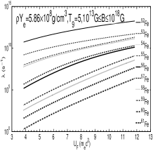
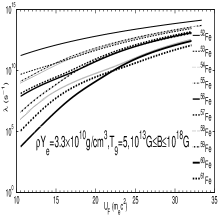
Figure 1: The EC rates for ^52-61 Fe as a function of the electron chemical potential at the density and temperature of $\rho Y_{e}=5.86\times 10^{8}g/cm^{3}$; $\rho Y_{e}=3.3\times 10^{10}g/cm^{3}$ and $T_{9}=5$

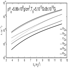
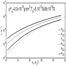
Figure 2: The EC rates for ^55-60 Co as a function of the electron chemical potential at the density and temperature of $\rho Y_{e}=5.86\times 10^{8}g/cm^{3}$; $\rho Y_{e}=3.3\times 10^{10}g/cm^{3}$ and $T_{9}=5$

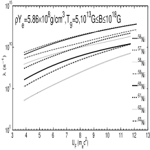
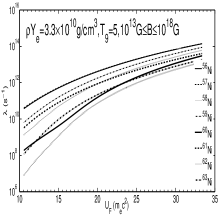
Figure 3: The EC rates for ^56-63 Ni as a function of the electron chemical potential at the density and temperature of $\rho Y_{e}=5.86\times 10^{8}g/cm^{3}$; $\rho Y_{e}=3.3\times 10^{10}g/cm^{3}$ and $T_{9}=5$

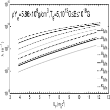
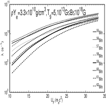
Figure 4: The EC rates for ^55-62 Mn as a function of the electron chemical potential at the density and temperature of $\rho Y_{e}=5.86\times 10^{8}g/cm^{3}$; $\rho Y_{e}=3.3\times 10^{10}g/cm^{3}$ and $T_{9}=5$

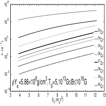
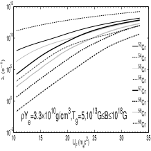
Figure 5: The EC rates for ^53-60 Cr as a function of the electron chemical potential at the density and temperature of $\rho Y_{e}=5.86\times 10^{8}g/cm^{3}$; $\rho Y_{e}=3.3\times 10^{10}g/cm^{3}$ and $T_{9}=5$

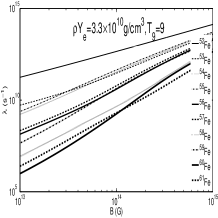
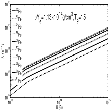
Figure 6: The EC rates for ^52-61 Fe as a function of the magnetic field at the density and temperature of $\rho Y_{e}=3.3\times 10^{10}g/cm^{3}$; $\rho Y_{e}=1.13\times 10^{14}g/cm^{3}$ and $T_{9}=9;15$ respectively

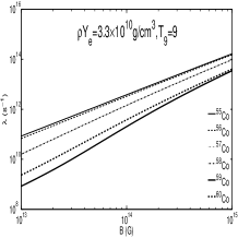
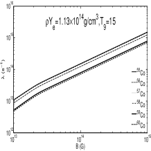
Figure 7: The EC rates for ^55-60 Co as a function of the magnetic field at the density and temperature of $\rho Y_{e}=3.3\times 10^{10}g/cm^{3}$; $\rho Y_{e}=1.13\times 10^{14}g/cm^{3}$ and $T_{9}=9;15$, respectively

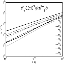
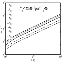
Figure 8: The EC rates for ^56-63 Ni as a function of the magnetic field at the density and temperature of $\rho Y_{e}=3.3\times 10^{10}g/cm^{3}$; $\rho Y_{e}=1.13\times 10^{14}g/cm^{3}$ and $T_{9}=9;15$ respectively

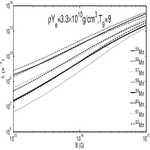
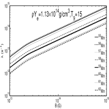
Figure 9: The EC rates for ^55-62 Mn as a function of the magnetic field at the density and temperature of $\rho Y_{e}=3.3\times 10^{10}g/cm^{3}$; $\rho Y_{e}=1.13\times 10^{14}g/cm^{3}$ and $T_{9}=9;15$ respectively

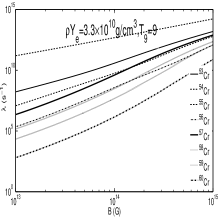
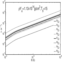
Figure 10: The EC rates for ^53-60 Cr as a function of the magnetic field at the density and temperature of $\rho Y_{e}=3.3\times 10^{10}g/cm^{3}$; $\rho Y_{e}=1.13\times 10^{14}g/cm^{3}$ and $T_{9}=9;15$ respectively

Figures 6–10 show the EC rates of some iron group nuclei as a function of the magnetic fields $B$ under the condition of $\rho Y_{e}=3.30\times 10^{10}g/cm^{3}$; $\rho Y_{e}=1.13\times 10^{14}g/cm^{3}$ and $T_{9}=9,15$ respectively. We find that the EC rates of most nuclides influenced greatly at relative lower temperature and density. For example, for most iron group nuclei (e.g. ^55-60 Co and ^56-63Ni ), the EC rates increase and even exceed by four orders of magnitude at $\rho Y_{e}=3.30\times 10^{10}g/cm^{3}$ and $T_{9}=9$. However, at $\rho Y_{e}=1.13\times 10^{14}g/cm^{3}$ and $T_{9}=15$ the increase is no more than by three orders of magnitude.

Comparing the results in these figures, it can be seen that the GT transition process of the EC process may not be dominant at lower temperature. This process is dominated by the low-energy transition. Therefore, the effect produced by this kind of densities is not very obvious in SMFs. We find that the distribution of the electron gas with high temperature and high density must satisfy the Fermi-Dirac distribution. The GT transition strength of nuclide is distributed in the form of the centrosymmetric Gaussian function about the GT resonance point. So the energies of the electrons taking part in the GT resonance transitions in the high–energy range are not symmetric in SMFs. The distribution of Gaussian function increases and includes more electrons to take part in the electron capture reactions. Therefore, with increasing of the temperature, it obviously accelerates the progress of the electron capture process. It inevitably leads to great increases of the EC rates.

Table 1: Comparisons of our calculations $\lambda^{B}_{ec}(\rm{LJ})$ in and not in SMFs for some typical iron group nuclides with those of FFN’s ($\lambda^{0}_{ec}(\rm{FFN}))$ and AUFD’s ($\lambda^{0}_{ec}(\rm{AUFD}))$, which are for the case without SMFs at $\rho_{7}=5.86,Y_{e}=0.47,T_{9}=3.4$.

$\lambda^{B}_{ec}(\rm{LJ})$
Nuclide	$\lambda^{0}_{ec}$(FFN)	$\lambda^{0}_{ec}$(AUFD)	$B_{12}=0$	$B_{12}=10$	$B_{12}=10^{3}$	$B_{12}=10^{6}$	$k1$	$k2$
56Ni	1.30e-2	1.60e-2	1.250e-2	3.9309e1	3.0078e3	1.2274e7	1.0400	1.2800
57Ni	9.93e-3	1.94e-2	1.573e-2	1.1020e1	4.5929e3	1.2513e7	0.6313	1.2333
58Ni	3.72e-4	6.36e-4	5.878e-4	1.6875e-1	1.9710e1	5.1269e5	0.6329	1.0820
59Ni	4.31e-3	4.37e-3	4.146e-3	2.2885e0	7.3434e3	7.5878e6	1.0396	1.0540
60Ni	9.17e-6	1.49e-6	1.287e-6	7.6940e-3	4.2441e0	2.4165e3	7.1251	1.1577
53Fe	3.91e-2	2.04e-2	1.889e-2	9.9095e1	2.2364e3	3.1121e6	2.0699	1.0799
54Fe	2.95e-4	3.11e-4	2.868e-4	7.4556e0	1.3858e2	3.7685e4	1.0286	1.0844
55Fe	1.57e-3	1.61e-3	1.357e-3	2.1021e0	2.0968e3	4.2672e6	1.1570	1.1864
55Co	1.36e-1	1.41e-1	1.336e-1	1.3468e3	1.2935e4	5.3337e6	1.0180	1.0554
56Co	6.91e-2	7.40e-2	7.026e-2	1.6156e1	9.2840e3	1.3409e7	0.9835	1.0532
57Co	3.50e-3	1.89e-3	7.026e-2	1.6156e1	9.2840e3	1.3409e7	2.1059	1.1372
58Co	9.93e-3	1.94e-2	1.680e-2	4.2633e2	1.1873e4	8.2574e6	0.5911	1.1548

Table 2: Comparisons of our calculations $\lambda^{B}_{ec}(\rm{LJ})$ in and not in SMFs for some typical iron group nuclides with those of FFN’s ($\lambda^{0}_{ec}(\rm{FFN}))$ and AUFD’s ($\lambda^{0}_{ec}(\rm{AUFD}))$, which are for the case without SMFs at $\rho_{7}=14.5,Y_{e}=0.45,T_{9}=3.80$.

$\lambda^{B}_{ec}(\rm{LJ})$
Nuclide	$\lambda^{0}_{ec}$(FFN)	$\lambda^{0}_{ec}$(AUFD)	$B_{12}=0$	$B_{12}=10$	$B_{12}=10^{3}$	$B_{12}=10^{6}$	$k1$	$k2$
57Co	1.04e-2	1.29e-2	1.0123e-2	1.0054e1	1.1138e3	1.5740e6	1.0274	1.2743
58Co	1.55e-2	3.07e-2	2.5604e-2	4.8841e1	1.9623e3	1.5610e6	0.6054	1.1990
59Co	5.44e-4	6.57e-4	4.3564e-4	1.5203e-1	1.1256e1	6.5784e5	1.2487	1.5081
60Co	1.15e-2	1.27e-2	1.0012e-2	3.5286e1	3.8400e3	7.1148e5	1.1486	1.2685
55Mn	2.03e-5	2.25e-5	2.1135e-5	6.4984e-3	2.7884e1	4.8910e4	0.9605	1.0646
56Mn	4.29e-5	2.56e-4	2.0552e-4	1.2549e-1	1.0288e1	6.1896e4	0.2087	1.2456
55Fe	1.21e-2	6.200e-3	5.7883e-3	3.1168e0	3.6345e2	9.2804e5	2.0904	1.0711
56Fe	2.81e-5	1.31e-6	1.2452e-6	2.2436e-3	3.0910e-1	4.1959e4	22.567	1.0520
57Fe	4.83e-5	1.84e-5	1.6534e-5	5.8381e-2	6.4230e0	4.7899e5	2.9213	1.1129
60Ni	1.39e-4	2.74e-5	2.3372e-5	3.4484e-2	2.0088e0	6.2462e5	5.9473	1.1723
61Ni	……	1.20e-3	1.0028e-3	3.0760e0	2.3054e2	6.6119e5	……	1.1966
53Cr	1.63e-5	2.46e-6	2.3225e-6	4.8821e-3	5.6122e-1	3.3553e4	7.0183	1.0592

Table 3: Comparisons of our calculations $\lambda^{B}_{ec}(\rm{LJ})$ in and not in SMFs for some typical iron group nuclides with those of FFN’s ($\lambda^{0}_{ec}(\rm{FFN}))$ and AUFD’s ($\lambda^{0}_{ec}(\rm{AUFD}))$, which are for the case without SMFs at $\rho_{7}=106,Y_{e}=0.43,T_{9}=4.93$.

$\lambda^{B}_{ec}(\rm{LJ})$
Nuclide	$\lambda^{0}_{ec}$(FFN)	$\lambda^{0}_{ec}$(AUFD)	$B_{12}=0$	$B_{12}=10$	$B_{12}=10^{3}$	$B_{12}=10^{6}$	$k1$	$k2$
55Mn	9.10e-3	8.73e-3	7.8895e-3	1.3770e2	3.1515e4	2.7488e6	1.1534	1.1065
56Mn	9.29e-3	2.90e-2	2.6762e-2	1.0681e2	6.4156e5	3.1205e6	0.8632	1.0836
57Mn	2.36e-5	4.03e-4	3.8320e-4	3.7901e1	2.1646e3	1.9839e5	0.1648	1.0517
58Mn	3.16e-4	2.94e-3	2.8113e-4	5.8219e2	1.3999e4	1.3999e6	0.1124	1.0458
59Fe	1.49e-4	1.83e-4	2.4663e-5	8.9315e2	7.7209e3	1.5121e5	0.6041	0.7420
61Ni	……	5.07e-1	3.3748e-1	2.2129e2	5.1440e4	2.2142e6	……	1.5023
63Ni	……	3.87e-3	2.5660e-3	1.2483e2	2.2122e3	1.3956e5	……	1.5082

Table 4: Comparisons of our calculations $\lambda^{B}_{ec}(\rm{LJ})$ in and not in SMFs for some typical iron group nuclides with those of FFN’s ($\lambda^{0}_{ec}(\rm{FFN}))$ and AUFD’s ($\lambda^{0}_{ec}(\rm{AUFD}))$, which are for the case without SMFs at $\rho_{7}=4010,Y_{e}=0.41,T_{9}=7.33$.

$\lambda^{B}_{ec}(\rm{LJ})$
Nuclide	$\lambda^{0}_{ec}$(FFN)	$\lambda^{0}_{ec}$(AUFD)	$B_{12}=0$	$B_{12}=10$	$B_{12}=10^{3}$	$B_{12}=10^{6}$	$k1$	$k2$
57Mn	4.29e2	8.36e2	7.6335e2	6.3917e4	2.9624e8	7.0466e10	0.5620	1.0952
58Mn	7.90e2	1.05e3	1.0326e3	4.6822e5	7.1383e9	4.1146e11	0.7651	1.0169
59Mn	……	1.41e2	1.0132e2	1.6386e3	1.3991e8	3.0604e10	……	1.3916
60Mn	……	2.55e2	1.1876e2	1.8443e4	2.6069e8	2.9223e10	……	2.1472
59Fe	7.43e2	7.20e2	6.1023e2	4.5585e4	5.7106e8	5.7106e10	1.2176	1.1799
60Fe	1.441e1	6.37e1	2.6867e1	1.0880e4	1.0880e8	3.3984e9	0.5363	2.3709
61Fe	……	1.63e2	1.4785e2	2.3397e3	4.5281e9	2.1010e10	……	1.1023
56Cr	……	3.33e1	2.8845e1	1.5366e3	6.4200e9	5.0816e9	……	1.1543
57Cr	……	6.09e1	3.9436e1	1.2695e3	7.5182e9	6.8590e9	……	1.5442

In summary, one can see that the lower the temperature and density, the less the effect on the EC rates from our numerical calculations. This is because the GT transitions processes are mainly aimed at in the high-energy region. Under the condition of lower temperature, the average kinetic energy of electrons is relatively small. The Fermi energy of electrons is also relatively lower at low density. And most electrons will be in the weakly degenerate state. The EC processes in the low–energy region make a comparatively large contribution, while the high–energy GT transition processes may not be dominated. On the contrary, the higher the temperature, the larger the average energy of electrons, the density and the Fermi energy of the electron gas become. The proportion occupied by the GT transition increases and the contribution to the rates may dominate.

According to above discussion, we can draw a conclusion that the SMFs has a significant influence on the EC rates for a given temperature-density point. Generally the higher the SMFs, the larger affect on the EC rates become. The reason is that the Fermi energy of electrons increases with the SMFs increasing and it may lead to more and more electrons whose energy is above the threshold for EC process. The results also show that the influences for different nuclei on EC reaction are different due to the different Q–values and transition orbits in SMFs.

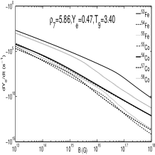
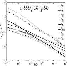
Figure 11: The RCEA as a function of the magnetic field at the density and temperature of $\rho_{7}=5.86,Y_{e}=0.47$; and $T_{9}=3.40$

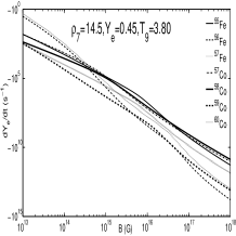
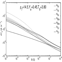
Figure 12: The RCEA as a function of the magnetic field at the density and temperature of $\rho_{7}=14.5,Y_{e}=0.45$; and $T_{9}=3.80$

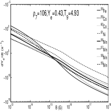
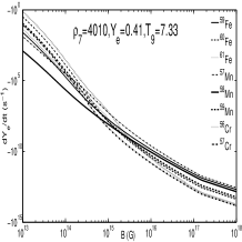
Figure 13: The RCEA as a function of the magnetic field at the density and temperature of $\rho_{7}=106,Y_{e}=0.43$; $T_{9}=7.93$ and $\rho_{7}=4010,Y_{e}=0.41$; $T_{9}=7.33$ respectively

As everyone knows, what really matters for stellar evolution is electronic abundance $Y_{e}$. Electronic abundance variation is one of crucial parameters in supernova. The electronic abundance serious influences the changes of electron degenerate pressure and entropy at late stages of stellar evolution, especially at the supernova explosion process and plays a very important role. Figures 11-13 show the RCEA due to EC of iron group nuclei as a function of magnetic field in SMFs. As seen in the three figures, SMFs have a large impact on the RCEA for most iron group nuclei. The $Y_{e}$ due to SMFs may be almost reduced more than eight orders of magnitude.

From above Figures, we can see the change of the electron fraction is very sensitivity parameter in EC process. The main reason resulted in the EC rates are increased greatly by SMFs. It may be induce the number of the electrons reduce largely. With increasing of the density and the magnetic field, the electron chemical potential becomes so high that rapid and great progress would be made due to large numbers of electrons join in EC reaction.

From the oxygen shell burning phase up to the end of convective core silicon burning phase of massive stars the EC rates on these nuclides play important roles. FFN had done some pioneer works on EC rates. In order to understand how much EC is affected by SMFs, the comparisons of our results $\lambda^{B}_{ec}$(LJ)in SMFs with those of FFN’s (Fuller et al., 1980, 1985)($\lambda^{0}_{ec}$(FFN)) and AUFD’s (Aufderheide et al., 1994)($\lambda^{0}_{ec}$ (AUFD)) for the case without SMFs are presented in tabular forms. Table 1-4 show the comparison of our results in SMFs with those FFN’s and AUFD’s in different astrophysical environments.

The calculated rates for most nuclides due to SMF are increased and even exceeded as much as for nine orders of magnitude of compared to FFN’s result, which for the case without SMFs. The four tables also show the comparisons of our results in SMFs with those and AUFD’s, which are for the case without SMFs. The calculated rates for most nuclides due to SMFs are increased and even exceeded as much as for eight orders of magnitude of compared to AUFD’s result.

For the case without SMFs the four tables show the comparison of calculated EC rates of our results with those FFN’s and AUFD’s. We find that our results are in well agreement with AUFD’s from the scale factor $k_{1}$ and $k_{2}$, but FFN’s are about close to one order magnitude bigger than ours.

The question about the blocking and thermal unblocking of final states in the process of EC, has discussed in detail by Langanke et al. (2001). Fuller et al. (1982) also show that all the corresponding neutron orbits are filled and the valence neutrons are in the $gd$–shell during collapse a point is reached where a average nucleus is so neutron-rich that, while the valence protons are still filling $pf$–shell orbits (Ray et al., 1984). However, we discuss the Gamow -Teller strength in stellar electron capture process on iron group nuclides based on $pf$–shell model in this paper. As an example, for ⁵⁸Co in process of EC, a proton is turned into a neutron by a GT transition and Fermi transition is blocked. All seven $pf$ protons are filled in the $1f_{7/2}$ orbital and thus the only allowed GT transitions are to the $1f_{7/2}$ and $1f_{5/2}$ neutron orbitals. The formal orbital is blocked by neutrons. Thus a $1f_{7/2}$ proton has become a $1f_{5/2}$ neutron.

On the other hand, the charge exchange reactions (p, n) and (n, p) make it possible to observe, in principle, the total GT strength distribution in nuclei. For some iron nuclides the experimental information is particularly rich and the availability of both $\rm{GT}^{+}$ and $\rm{GT}^{-}$. It makes possible to study in detail the problem of renormalization of $\sigma\tau$ operators. The total calculated GT strength in a full $pf$–shell calculation, resulting in $\rm{B}(\rm{GT})=g_{A}^{2}|\langle\vec{\sigma}\tau_{+}\rangle|^{2}$, where $g_{\rm{A}}^{2}$ is axial-vector coupling constant(Langanke & Martinez-Pinedo., 1998).

For example, the electron capture on ⁵⁶Ni is dominated by the wave functions of the parent and daughter states and effected greatly by SMFs. And the total GT strength for ⁵⁶Ni in a full $pf$–shell calculation, resulting in $\rm{B}(\rm{GT})=10.1g_{A}^{2}$. The total GT strength of the other important nuclide ⁵⁶Fe in a full $pf$–shell calculation can be found in the Ref. (Caurier et al., 1995). An average of the GT strength distribution is in fact obtained by SMMC method.

The electron capture of the neutron rich nuclide do not has measured mass, so that the EC Q-value has to be estimated with a mass formal by FFN. FFN used the Seeger & Howard. (1975) Semiempirical atomic mass formula, so that the Q-value used in the effective rates are quite different. On the basis of the independent particle model, FFN parametrized the GT contribution to the EC rates. To complete the FFN rate estimate, the GT contribution has been supplemented by a contribution simulating low-lying transitions. Basing on nuclear shell model, AUFD expanded the FFN’s works and analyzed the nuclear excited level by a Simple calculation on the nuclear excitation level transitions in their works. The capture rates are made up of the lower energy transition rates between the ground states and the higher energy transition rates between GT resonance states. Their work simplifies the nuclear excited energy level transition calculation, Thus the calculation method is a little rough.

It is generally known that the EC rate is easily calculated as long as the distribution of nuclear excited states is clear. But it is very difficult to know the distribution because a lot of nuclear excited states are not stable at the stage of supernova explosive. The experimental data on GT distribution within the nucleus becomes available. These data show that the EC value of the FFN’s works (Fuller et al., 1980, 1985), which using the GT contribution parameters have large errors. These data clearly show that the GT strength disappear in the daughter nucleus and split into several excitation. AUFD analyze the nuclear excited level by a Simple calculation on the nuclear excitation level transitions in their works. The excited state is splinted up into the ground state near the low energy parts and resonant states near the high-energy parts respectively. Therefore, the capture rates are made up of the lower energy transition rates between the ground states and the higher energy transition rates between GT resonance states. Therefore the works of AUFD is an oversimplification and the accuracy is limited.

4 Conclusions

As everyone knows, the problems about the influence of a strong magnetic field on electron capture in non-zero temperature crusts of neutron stars have already been discussed by Dai et al. (1993); Luo & Peng (1997). Their results show that the magnetic fields ($10^{9}-10^{13}G$) on surfaces of neutron stars have almost no effect on the electron capture rate. In this paper, we have carried out estimation for EC rates and RCEA of iron group nuclei in SMFs which is ranging from $10^{13}G$ to $10^{18}G$. It is concluded that an SMFs has a significant effect on them For most iron group nuclides.

We also compare our results with those of FFN’s and AUFD’s for the case with and without SMFs. The results show that our results is in well agreement with AUFD’s, but the FFN’s are about close to one order magnitude bigger than ours for the case without SMFs. On contrary, our calculated rates for most nuclides in SMFs are increased and even exceeded as much as by nine and eight orders of magnitude bigger than FFN’s and AUFD’s, which are in case without SMFs, respectively.

As is known to all, the research on EC reaction at late stages of stellar evolution will still be a long-term and arduous task. It will have a key and profound significance to better understand and study the final evolutionary paths and nuclear interaction model of cosmic objects, as well as the physical structure and state in the interiors of celestial objects in the environment of high temperature, high pressure, high magnetic fields and high density. Our conclusions may be helpful to the investigation of the late evolution of the neutron stars and magnetars, the nucleosyntheses of heavy elements and the numerical calculations of stellar evolution.

References

- Aufderheide et al. (1994) Aufderheide M. B.,Fushikii I., Woosely S. E. and Hartmanm D. H., 1994, ApJ.S, 91, 389
- Aufderheide et al. (1990) Aufderheide M. B. Brown G. E., Kuo T. T. S., Stout D. B., and Vogel P., 1990, ApJ, 362, 241
- Akhiezer & Berestetskii. (1981) Akhiezer A. I., and Berestetskii V. B., 1981, ”Quantum Electrodynamics,” M: Nauka., Appendix A2, 422
- Baym et al. (1998) Baym, G., Pethick, C., and Ann, J., 1975, ARNPS, 25, 27
- Caurier et al. (1995) Caurier E. Martinez-Pinedo G., Poves A., and Zuker A. P., 1995, Phys. Rev. C., 52, 1736
- Dean et al. (1998) Dean D. J., Langanke K., Chatterjee L., Radha P. B. and Strayer M. R., 1998, Phys. Rev, 58, 536
- Dai et al. (1993) Dai Z. G., Lu T., and Peng Q. H., 1993, A&A, 272, 705
- Fuller et al. (1980) Fuller G. M., Fowler W. A. and Newman M. J., 1980, ApJ.S, 42, 447
- Fuller et al. (1985) Fuller G. M., Fowler W. A. and Newman M. J., 1985, ApJ, 293, 1
- Fuller et al. (1982) Fuller G. M., Fowler W. A. and Newman M. J., 1982, ApJ, 252, 715
- Gao et al. (2011) Gao Z. F., Peng Q. H., Wang N., Chou C. K., Huo W. S., 2011, ApS&S., 336, 427
- Langanke et al. (2001) Langanke K., Kolbe E., Dean D. J., 2001, Phys. Lett. C., 63, 032801
- Langanke & Martinez-Pinedo. (1998) Langanke K. and Martinez-Pinedo G., 1998, Phys. Lett. B., 436, 19
- Luo & Peng (1997) Luo Z. Q. and Peng Q. H., 1997, ChA&A, 21, 254
- Liu & Luo. (2007a) Liu J. J. and Luo. Z. Q., 2007a, Chin. Phys., 16, 2671
- Liu & Luo. (2007b) Liu J. J. and Luo. Z. Q., 2007b, Chin. Phys., 16, 3624
- Liu & Luo. (2008a) Liu J. J. and Luo. Z. Q., 2008a, Chin.Phys. C., 32, 108
- Liu & Luo. (2008b) Liu J. J. and Luo. Z. Q., 2008b, Comm.Theo. Phys., 49, 239
- Liu et al. (2007) Liu J. J. Luo. Z. Q., Liu H. L., and Lai X. J., 2007, IJMPA, 22, 3305
- Liu. (2013a) Liu J. J., 2013a, MNRAS., 433, 1108
- Liu. (2013b) Liu J. J., 2013b, ApS&S., 343, 579
- Liu. (2013c) Liu J. J., 2013c, ApS&S., 343, 117
- Liu. (2013d) Liu J. J., 2013d, RAA., 13, 99
- Liu. (2013e) Liu J. J., 2013e, RAA., 13, 945
- Liu. (2013f) Liu J. J., 2013f, Chin.Phys. C., 37, 085101
- Liu. (2012) Liu J. J., 2012, Chin. Phys. Lett., 29, 122301
- Peng & Tong (2007) Peng Q. H. and Tong H., 2007, MNRAS, 378, 159
- Peng et al. (2012) Peng Q. H., Gao Z. F.,and Wang, N., 2012, AIP Conference Proceedings., 1484, 467
- Ray et al. (1984) Ray A., Chitre S. M., Kar K., 1984, ApJ, 285, 766
- Seeger & Howard. (1975) Seeger P. A. and Howard W. M., 1975, Nuclear Phys. A., 238, 491
- Thielemann et al. (1986) Thielemann Friedrich-Karl., Truran James. W. and Arnould Marcel., 1986, Advances in nuclear astrophysics; Proceedings of the Second IAP Workshop., 525, 540