Asymmetric band widening by screened exchange competing with local correlations in SrVO₃: new surprises on an old compound from combined GW and dynamical mean field theory GW+DMFT

Abstract

The very first dynamical implementation of the combined GW and dynamical mean field scheme “GW+DMFT” for a real material was achieved recently [J.M. Tomczak et al., Europhys. Lett. 2012], and applied to the ternary transition metal oxide SrVO₃. Here, we review and extend that work, giving not only a detailed account of full GW+DMFT calculations, but also discussing and testing simplified approximate schemes. We give insights into the nature of exchange and correlation effects: Dynamical renormalizations in the Fermi liquid regime of SrVO₃ are essentially local, and nonlocal correlations mainly act to screen the Fock exchange term. The latter substantially widens the quasi-particle band structure, while the band narrowing induced by the former is accompanied by a spectral weight transfer to higher energies. Most interestingly, the exchange broadening is much more pronounced in the unoccupied part of spectrum. As a result, the GW+DMFT electronic structure of SrVO₃ resembles the conventional density functional based dynamical mean field (DFT+DMFT) description for occupied states, but is profoundly modified in the empty part. Our work leads to a reinterpretation of inverse photoemission spectroscopy (IPES) data. Indeed, we assign a prominent peak at about 2.7 eV dominantly to e_g states, rather than to an upper Hubbard band of t_2g character. Similar surprises can be expected for other transition metal oxides, calling for more detailed investigations of the conduction band states.

I Introduction

Within the last decade, a new research field has developed at the interface of many-body theory and first principles electronic structure calculations. The aim is the construction of materials-specific parameter-free many-body theories that preserve the ab initio nature of density functional based methods, but incorporate at the same time a many-body description of Coulomb interactions beyond the independent-electron picture into computational approaches for spectroscopic or finite-temperature properties.

Historically, the first non-perturbative electronic structure techniques for correlated materials evolved from many-body treatments of the multi-orbital Hubbard Hamiltonian with realistic parameters. The general strategy of these so-called “LDA++” approaches Lichtenstein and Katsnelson (1998); Anisimov et al. (1997) (for reviews see, e.g., Biermann (2006); Held et al. (2006); ani (2000); Kotliar and Vollhardt (2004)) consists in the extraction of the parameters of a many-body Hamiltonian from first principles calculations and then solving the problem by many-body techniques. In practice, this procedure has met tremendous success in the description of the electronic structure of correlated materials, for a wide range of materials, from transition metals Lichtenstein et al. (2001); Biermann et al. (2004a), their oxides Liebsch (2003); Pavarini et al. (2004); Held et al. (2001a); Keller et al. (2004); Poteryaev et al. (2007); Nekrasov et al. (2005); Tomczak and Biermann (2009a); Nekrasov et al. (2006); Saha-Dasgupta et al. (2005); Rodolakis et al. (2010); Hansmann et al. (2012); Wang et al. (2012); Zhang et al. (2012); Flesch et al. (2012); Gorelov et al. (2010); Pavarini and Koch (2010); De Raychaudhury et al. (2007); Kuneš et al. (2009); Augustinský et al. (2013); Biermann et al. (2005); Tomczak and Biermann (2009b, c), sulphides Lechermann et al. (2005, 2007), or silicides Tomczak et al. (2012a, 2013a), to $f$-electron compounds Miyake et al. (2008); Tomczak et al. (2013b); Savrasov et al. (2001); Held et al. (2001b). More recently, iron pnictide compounds (see e.g. Refs. Haule et al., 2008; Skornyakov et al., 2009; Anisimov et al., 2009; Aichhorn et al., 2009, 2010; Hansmann et al., 2010; Lee et al., 2010; Ferber et al., 2012; Werner et al., 2012) or spin-orbit materials Martins et al. (2011) have come into the focus of many-body electronic structure calculations, emphasizing the need for fully ab initio techniques, including a first principles description of the effective Coulomb interactions. The challenge here is an accurate description of screening of low-energy interactions by high-energy degrees of freedom, as well as the screening of local interactions by nonlocal charge fluctuations Ayral et al. (2012, 2013); Hansmann et al. (2013).

Despite the tremendous success of LDA++ schemes, one should be aware of the fact that the ambiguities in the construction of the Hamiltonian are not limited to the many-body part: not even the use of the Kohn-Sham band structure of DFT as a starting Hamiltonian has a direct microscopic justification beyond heuristic arguments. Though renormalization group techniques suggest that in many cases the relevant low-energy effective Hamiltonian can indeed be cast into a generalized (multi-orbital) Hubbard form, in practice neither the precise form nor the parameters can be derived directly from the Coulomb Hamiltonian in the continuum. In this sense, the construction of an “LDA++” Hamiltonian amounts to a rather ad hoc combination of a Kohn-Sham Hamiltonian and multi-orbital Hubbard (and Hund) interaction terms for a subset of “correlated orbitals”. Conceptually, there is moreover a mismatch arising from the fact that the full long-range Coulomb interactions enter the one-particle part of the Hamiltonian (even if only in a mean-field fashion), while in the many-body part they are replaced by effective local interactions acting only in a low-energy subspace. This has two consequences. The first – well-known one – is related to the double counting correction: Correlation effects accounted for in the exchange-correlation potential of DFT have to be subtracted. Yet, a microscopically motivated definition of this term is, even on a conceptual level, impossible. The second one is more subtle, and has only recently started to receive some attention: in fact, the same processes that screen the effective Coulomb interactions are also responsible for renormalizations of the one-body part of the Hamiltonian. This can be understood from an analysis of screening as resulting from coupling of the electrons to bosonic excitations, such as plasmons, particle-hole excitations or more complex many-body processes. The diagonalization of the corresponding electron-boson Hamiltonian results in fermionic quasi-particles (“electronic polarons”) corresponding to electrons dressed by their screening bosons, and thus having heavier masses. This mass enhancement corresponds to an effective renormalization of their kinetic energy, and hence of the one-body part of the Hamiltonian. This kind of effect has recently been demonstrated explicitly Casula et al. (2012a) on the basis of the constrained random phase approximation (cRPA), which allows for an explicit (yet approximate) estimation of dynamical Hubbard interactions in solids Aryasetiawan et al. (2004a). The corresponding one-body renormalizations have been investigated in the framework of dynamical mean field theory (DMFT) for SrVO₃ Casula et al. (2012b) and BaFe₂As₂ Werner et al. (2012), and a low-energy effective Hamiltonian comprising these renormalizations has been derived in Ref. Casula et al., 2012a.

In addition to these effects related to the long-range nature of the Coulomb interactions and the resulting quantum dynamical screening, in practice, yet another difficulty arises when proceeding to (approximate) many-body solutions of the multi-orbital Hubbard Hamiltonian. Indeed, while the construction of the one-body part of the Hamiltonian (within DFT) naturally puts the electronic density at the center of the attention, many-body theory is most readily formulated within a Green’s function language. This mismatch in language is the final capstone that ensures that matching contributions between the effective one-body Hamiltonian and the many-body terms are truly impossible to identify.

Ideally, the desired specifications of new many-body electronic structure techniques beyond “LDA++” approaches can thus be summarized in three main requirements:

• The theory should be entirely formulated in the Green’s function language, even at the one-body level.

• The theory should deal directly with the long-range Coulomb interactions, and any effective local “Hubbard-like” interactions should arise only as intermediate auxiliary quantities.

• At the same time, the theory should retain the non-perturbative character of dynamical mean field theory, thus avoiding limitations due to a truncation of the perturbation series. This latter point is essential to ensure the scheme to be equally appropriate in the weak, strong and intermediate coupling regimes.

The combination of Hedin’s GW approximation – many-body perturbation theory to first order in the screened Coulomb interaction $W$ – and dynamical mean field theory meets these criteria. Such a scheme was proposed a decade ago Biermann et al. (2003), based on the construction of the free energy of a solid as a functional of the Green’s function $G$ and $W$.

Only very recently have practical implementations for real materials been achievedTomczak et al. (2012b); Hansmann et al. (2013) that go beyond simple static approximation schemes Biermann et al. (2003); Karlsson (2005); Taranto et al. (2013). The reason was the necessity of dealing with frequency-dependent interactions at the DMFT level, which has remained a major bottleneck until recently. Recent advances in Monte Carlo techniquesWerner and Millis (2010) and the invention of a reliable cumulant-type scheme, the “Bose factor ansatz” Casula et al. (2012b), have unblocked the situation: two calculations within GW+DMFT taking into account dynamical interactions have been achieved recently, for SrVO₃ Tomczak et al. (2012b) and for systems of adatoms on surfaces Hansmann et al. (2013). In this work, we review and extend the former calculations, giving a detailed account of fully dynamical GW+DMFT calculations for SrVO₃. The paper is organised as follows: In Sect. II, we give an extensive summary of the concepts of the combined GW+DMFT scheme and discuss aspects of its practical implementation, in particular related to the Bose factor ansatz. Furthermore, we devote an extensive discussion to the question of how to treat multi-orbital materials: we propose that for ligand and conduction band shells a perturbative treatment might be sufficient, and show how such a procedure can be combined with the non-perturbative DMFT treatment of the low-energy correlated shells. In Sect. III, we review the electronic structure of our target compound, pointing out problems left open within conventional LDA++ schemes. Section IV presents the results of fully dynamical GW+DMFT calculations, in comparison to GW calculations, LDA+DMFT with static and dynamic interactions, and to simplified combinations of GW and DMFT which allow for a detailed analysis of the importance of the different terms entering the theory. We discuss the implications of our results in Section V, before arriving at our conclusions in Sect. VI.

II The “GW+DMFT” Methodology

II.1 Overview

The starting point of the GW+DMFT scheme is Hedin’s GW approximation (GWA)Hedin (1965), in which the self-energy of a quantum many-body system is obtained from a frequency convolution (or product in time) of the Green’s function G with the screened Coulomb interaction $W=\epsilon^{-1}V$. The dielectric function $\epsilon$, which screens the bare Coulomb potential $V$, is – within a pure GW scheme – obtained from the random phase approximation. The GW+DMFT scheme, as proposed in Biermann et al. (2003), combines the first principles description of screening inherent in GW methods with the non-perturbative nature of DMFT, where local quantities such as the local Green’s function are calculated to all orders in the interaction from an effective reference system (“impurity model”). In DMFT, one imposes a self-consistency condition for the one-particle Green’s function, namely, that its on–site projection equals the impurity Green’s function. In GW+DMFT, the self-consistency requirement is generalized to encompass also two-particle quantities, namely, the local projection of the screened interaction is required to equal the impurity screened interaction. This in principle promotes the Hubbard U from an adjustable parameter in DMFT techniques to a self-consistent auxiliary function that incorporates long-range screening effects in an ab initio fashion. Indeed, as already alluded to above, not only higher energy degrees of freedom can be downfolded into an effective dynamical interaction, but one can also aim at incorporating nonlocal screening effects into an effective dynamical $\mathcal{U}(\omega)$. The theory is then free of any Hubbard parameter, and the interactions are directly determined from the full long-range Coulomb interactions in the continuum.

From a formal point of view, the GW+DMFT method, as introduced in Biermann et al. (2003), corresponds to a specific approximation to the correlation part of the free energy of a solid, expressed as a functional of the Green’s function G and the screened Coulomb interaction W: the nonlocal part is taken to be the first order term in $W$, while the local part is calculated from a local impurity model as in (extended) dynamical mean field theory. This leads to a set of self-consistent equations for the Green’s function $G$, the screened Coulomb interaction $W$, the self-energy $\Sigma$ and the polarization $P$ Biermann et al. (2004b); Aryasetiawan et al. (2004b). Specifically, the self-energy is obtained as $\Sigma=\Sigma^{local}+\Sigma^{nonlocal}_{GW}$, where the local part $\Sigma_{local}$ is derived from the impurity model. In practice, however, the calculation of a self-energy for (rather delocalized) s- or p-orbitals has never been performed within DMFT, and it appears to be more physical to approximate this part also by a GW-like expression. For these reasons Ref. Tomczak et al., 2012b proposed a practical scheme, in which only the local part of the self-energy of the “correlated” orbitals is calculated from the impurity model and all other local and nonlocal components are approximated by their first order expressions in $W$.

In the following subsections, we first briefly summarize the functional formulation of the GW, DMFT and GW+DMFT schemes from a general point of view (section II.2). The corresponding GW+DMFT equations are summarized in appendix A. Sections II.3 and II.4 are devoted to the “orbital-separated scheme” implemented for SrVO₃, defining the equations solved in practice. We then review the dynamic atomic limit approximation for the solution of dynamical impurity models (section II.5), while section II.6 summarizes some technicalities.

II.2 Unified view on GW, DMFT, and GW+DMFT

Within the Born-Oppenheimer approximation, the electronic many-body states in a solid are determined by the eigenstates of the Coulomb Hamiltonian

$$H=H_{kin}+H_{pot}+H_{ee}$$ (1)

where the first two terms denote the kinetic energy part and one-body potential created by the ions respectively. The last term, $H_{ee}=\sum_{nmn^{\prime}m^{\prime}}v_{nmn^{\prime}m^{\prime}}a^{\dagger}_{n}a^{\dagger}_{m}a_{m^{\prime}}a_{n^{\prime}}$, with $v_{nmn^{\prime}m^{\prime}}=\langle nm|\frac{1}{|r-r^{\prime}}|n^{\prime}m^{\prime}\rangle$ the matrix elements of the Coulomb interaction in the continuum, denotes the electron-electron interaction.

Following Almbladh et al.ALMBLADH et al. (1999), the free energy of a solid can be formulated as a functional $\Gamma[G,W]$ of the Green’s function $G$ and the screened Coulomb interaction $W$ of the solid. The latter is defined as the correlation function of bosonic excitations corresponding to density fluctuations, that is, in mathematical terms, as the propagator of the Hubbard-Stratonovich field decoupling the Coulomb interaction term. The GW method, dynamical mean field theory and the combined GW+DMFT scheme can then be viewed as different approximations to this $\Gamma[G,W]$ functional.

The functional $\Gamma$ can trivially be split into a Hartree part $\Gamma_{H}$ and a many body correction $\Psi$, which contains all corrections beyond the Hartree approximation : $\Gamma=\Gamma_{H}+\Psi$. The Hartree part can be given in the form

$$\Gamma_{H}[G,W] = Tr\ln G-Tr[({G_{H}}^{-1}-G^{-1})G]$$ (2)

$$- \frac{1}{2}Tr\ln W+\frac{1}{2}Tr[({V_{q}}^{-1}-W^{-1})W]$$

with $G_{H}$ being the Hartree Green’s function, and $V_{q}$ the Fourier transform of the bare Coulomb interaction. The $\Psi$-functional is the sum of all skeleton diagrams that are irreducible with respect to both one-electron propagator and interaction lines. $\Psi[G,W]$ has the following properties:

$$\frac{\delta\Psi}{\delta G}=\Sigma^{xc}$$

$$\frac{\delta\Psi}{\delta W}=P.$$ (3)

The $\Psi$ functional was first derived in ALMBLADH et al. (1999). A detailed discussion in the context of extended DMFT can be found in Ref. Chitra and Kotliar, 2001, while Refs. Biermann et al., 2003, 2004b; Aryasetiawan et al., 2004b view it from the GW+DMFT point of view.

An elegant derivation (see e.g. Biermann et al., 2004b; Aryasetiawan et al., 2004b; Hansmann et al., 2013) of the Almbladh free energy functional is obtained through a Hubbard Stratonovich decoupling of the interaction term by a bosonic field $\phi$, the introduction of Lagrange multipliers $\Sigma$ and $P$ imposing $\langle cc^{\dagger}\rangle$ and $\langle\phi\phi\rangle$ to equal externally chosen fermionic and bosonic propagators $G$ and $W$, and finally a Legendre transformation to obtain a functional of the latter two quantities.

The GW approximation consists in retaining the first order term in the screened interaction $W$ only, thus approximating the $\Psi$-functional by

$$\Psi[G,W]=-\frac{1}{2}Tr(GWG).$$ (4)

We then trivially find

$$\Sigma^{xc}=\frac{\delta\Psi}{\delta G}=-GW$$ (5)

$$P=\frac{\delta\Psi}{\delta W}=GG.$$ (6)

Extended DMFTHendrik (1996); Si and Smith (1996); Sengupta and Georges (1995), on the other hand, would calculate all local quantities that should be derived from this functional from a local impurity model. One can thus formally write

$$\Psi\,=\,\Psi_{imp}[G^{loc},W^{loc}].$$ (7)

The combined GW+DMFT scheme Biermann et al. (2003) consists in approximating the $\Psi$ functional as a direct combination of local and nonlocal parts from GW and extended DMFT, respectively:

$$\Psi\,=\,\Psi_{GW}^{\rm{non-loc}}[G,W]+\Psi_{imp}[G^{loc},W^{loc}]$$ (8)

More explicitly, the nonlocal part of the GW+DMFT $\Psi$-functional is given by

$$\Psi_{GW}^{\rm{non-loc}}[G,W]=\Psi_{GW}[G,W]-\Psi_{GW}^{\rm{loc}}[G,W]$$ (9)

while the local part is taken to be an impurity model $\Psi$ functional. Following (extended) DMFT, this on-site part of the functional is generated from a local quantum impurity problem. The expression for its free energy functional $\Gamma_{imp}[G_{imp},W_{imp}]$ is analogous to (2) with the Weiss field ${\cal G}$ replacing ${G_{H}}$ and the Hubbard ${\cal U}$ replacing $V$ :

$$\Gamma_{imp}[G_{imp},W_{imp}] = Tr\ln G_{imp}-Tr[({\cal G}^{-1}-G_{imp}^{-1})G_{imp}]$$ (10)

$$- \frac{1}{2}Tr\ln W_{imp}+\frac{1}{2}Tr[({\cal U}^{-1}-W_{imp}^{-1})W_{imp}]$$

$$+ \Psi_{imp}[G_{imp},W_{imp}]$$

The impurity quantities $G_{imp},W_{imp}$ can thus be calculated from the effective action:

$$S =\int d\tau d\tau^{\prime}\left[-\sum c^{\dagger}_{L}(\tau){\cal G}^{-1}_{LL^{\prime}}(\tau-\tau^{\prime})c_{L^{\prime}}(\tau^{\prime})\right.$$

$$+ \frac{1}{2}\left.\sum:c^{\dagger}_{L_{1}}(\tau)c_{L_{2}}(\tau):{\cal U}_{L_{1}L_{2}L_{3}L_{4}}(\tau-\tau^{\prime}):c^{\dagger}_{L_{3}}(\tau^{\prime})c_{L_{4}}(\tau^{\prime}):\right]\hskip-28.45274pt$$

where the sums run over all orbital indices $L$. In this expression, $c_{L}^{\dagger}$ is a creation operator associated with a localized orbital $L$, and the double dots denote normal ordering (taking care of Hartree terms). For simplicity, we restrict the discussion to the paramagnetic case and omit any spin indices.

The construction (8) of the $\Psi$-functional is the only ad hoc assumption in the GW+DMFT approach. The explicit form of the GW+DMFT equations follows then directly from the functional relations between the free energy, the Green’s function, the screened Coulomb interaction etc. Taking derivatives of the functional (8) as in (II.2) yields the complete self-energy and polarization operators:

$$\Sigma^{xc}({\bf k},i\omega_{n})_{LL^{\prime}} = \Sigma_{GW}^{xc}({\bf k},i\omega_{n})_{LL^{\prime}}$$

$$- \sum_{\bf k}\Sigma_{GW}^{xc}({\bf k},i\omega_{n})_{LL^{\prime}}+[\Sigma^{xc}_{imp}(i\omega_{n})]_{LL^{\prime}}$$

$$P({\bf q},i\nu_{n})_{\alpha\beta} = P_{GW}({\bf q},i\nu_{n})_{\alpha\beta}$$

$$- \sum_{\bf q}P_{GW}({\bf q},i\nu_{n})_{\alpha\beta}+P_{imp}(i\nu_{n})_{\alpha\beta}$$

Here, Greek letters indicate a two-particle basis, constructed from the localized (Wannier) basis indexed by $L$. The ad hoc combination of the functional $\Psi$ constructed as a sum of local and nonlocal parts thus leads to a physically attractive result: The off-site part of the self-energy (II.2) is taken from the GW approximation, whereas the on-site part is calculated to all orders from the dynamical impurity model. This treatment thus goes beyond usual extended DMFT, where the lattice self-energy and polarization are just taken to be their impurity counterparts. The second term in (II.2) subtracts the on-site component of the GW self-energy thus avoiding double counting. At self-consistency this term can be rewritten as:

$$\sum_{\bf k}\Sigma_{GW}^{xc}({\bf k},\tau)_{LL^{\prime}}=-\sum_{L_{1}L_{1}^{\prime}}{W_{imp}}(\tau)_{LL_{1}L^{\prime}L^{\prime}_{1}}{G_{imp}}(\tau)_{L^{\prime}_{1}L_{1}}$$ (14)

so that it precisely subtracts the contribution of the GW diagram to the impurity self-energy. Similar considerations apply to the polarization operator.

The general set of GW+DMFT equations to be solved self-consistently is summarized in Appendix A. In the following, we discuss a variant, which allows for a physically motivated cheaper treatment of ligand and itinerant empty states.

II.3 The “orbital-separated” GW+DMFT scheme

In the original GW+DMFT scheme as described in Ref. Biermann et al., 2003, the $\Psi$ functional is decomposed into nonlocal and local parts, which are then approximated by GW and DMFT respectively. This means that the local physics of all valence orbitals, including rather itinerant $s$ or $p$ states, would be generated from a self-consistent impurity model. It stands to reason that the self-consistent dynamical $\mathcal{U}$ for those orbitals would in fact come out to be rather small, so that the local dynamical contribution to the self-energy is also small and well described by its first order term in $W$. In practice, the self-energy for the itinerant states would thus be well described by a perturbative self-energy, that is by the GW self-energy for both, local and nonlocal parts.

In view of these considerations, it seems a waste of computing time to attempt to solve a dynamical impurity models for all valence states, since the same result can be obtained by applying the DMFT construction only to a subset of “correlated” states, and to treat all others entirely by GW. A scheme along these lines was proposed and implemented in Ref. Tomczak et al., 2012b.

The equations for the self-energy and polarization are in this case replaced by

$$\Sigma^{xc}({\bf k},i\omega_{n})_{LL^{\prime}} = \Sigma_{GW}^{xc}({\bf k},i\omega_{n})_{LL^{\prime}}$$

$$- \sum_{\bf k}\Sigma_{GW}^{xc,d}({\bf k},i\omega_{n})_{LL^{\prime}}+[\Sigma^{xc,d}_{imp}(i\omega_{n})]_{LL^{\prime}}$$

$$P({\bf q},i\nu_{n})_{\alpha\beta} = P_{GW}({\bf q},i\nu_{n})_{\alpha\beta}$$

$$- \sum_{\bf q}P_{GW}^{d}({\bf q},i\nu_{n})_{\alpha\beta}+P_{imp}^{d}(i\nu_{n})_{\alpha\beta}$$

where the superscript $d$ denotes the projection onto the low-energy correlated space.

One may be tempted to redefine the $\Psi$ functional as the one of the GW approximation $GWG$, corrected for its local part by DMFT only within the correlated subspace (denoted here as $d$), as follows:

$$\Psi[G,W]=GWG - G^{loc,d}W^{loc,d}G^{loc,d}$$ (17)

$$+ \Psi_{imp}[G^{loc,d},W^{loc,d}]$$

or, alternatively, by keeping the original decomposition into local and nonlocal parts

$$\Psi[G,W]=\Psi^{nonlocal}+\Psi^{local}$$ (18)

but approximating the local one by a combination of GW and DMFT

$$\Psi^{loc}[G,W]=G^{loc}W^{loc}G^{loc} - G^{loc,d}W^{loc,d}G^{loc,d}$$ (19)

$$+ \Psi_{imp}[G^{loc,d},W^{loc,d}].$$

Here, the superscript $loc$ denotes the projection on the local component, and $d$ the projection onto the correlated subspace.

Though appealing at first sight, such combinations cannot be justified without further approximations on a functional basis. This is due to the fact that screening couples the correlated and itinerant subspaces, so that “downfolding” of the interactions to obtain an effective bare interaction within the correlated subspace necessarily involves a decoupling approximation. In the functionals above, this is born out of the difficulty of defining $W^{loc,d}$, as well as of postulating that $\Psi_{imp}$ is a functional of the Green’s function and screened Coulomb interaction of the correlated subspace only.

Fortunately, in practice, these conceptual difficulties do not prevent us from identifying a well-defined scheme, that corresponds to a combination of GW and DMFT, where the impurity model is used for the correlated space only. The application to SrVO₃ presented below confirms the accuracy of such a scheme. In the following subsection we therefore describe the “orbital-separated scheme” used in the present work, where only the local part of the self-energy of the “correlated” orbitals is calculated from the impurity model and all other local and nonlocal components are approximated by their first order expressions in $W$.

II.4 Orbital-separated scheme: the Equations

For the reasons discussed above, in the orbital-separated scheme, one deviates from the general prescription Eqs. (II.2-II.2) for the self-energy and polarization by replacing their local parts by their counterparts generated from an impurity model within the correlated subspace only. We outline in the following the iterative loop obtained at the one-shot GW level but with full self-consistency at the impurity level. We call the correlated subspace $d$-space and its complement the $r$-space. Projections onto these spaces are noted by superscripts. We furthermore assume that we dispose of a Wannier basis which blockdiagonalizes the full LDA Hamiltonian, and that the GW self-energy is block-diagonal in the same basis. The Wannier basis can be thought of as obtained from the construction of maximally localized Wannier functions in the $d$ and in the $r$ space separately. The assumption of a vanishing GW self-energy block $\Sigma^{dr}$ in this basis is an additional approximation, Aryasetiawan et al. (2009) which is however very accurate, as we have explicitly verified for our target compound SrVO₃. We note that the common assumption in GW calculations of a diagonal self-energy in the Kohn-Sham basis is in fact a less justified approximation, and even this is not a severe restriction for SrVO₃ Taranto et al. (2013).

Starting with a guess for the Weiss field and the auxiliary Hubbard $\mathcal{U}$, the impurity model is solved, that is the impurity Green’s function $G_{imp}$ and screened Coulomb interaction $W_{imp}$ are obtained. These are matrices in the orbital space of the correlated states only. In order to obtain the full self-energy and polarization the combined quantities

$$\Sigma=\Sigma_{GW}-\Sigma_{GW}^{loc,d}+\Sigma_{imp}$$ (20)

$$P=GG-G^{loc,d}G^{loc,d}+P_{imp}$$ (21)

involve “upfolding” to the full Hilbert space.

Then, the self-consistency equations for the determination of the Weiss mean-field and the auxiliary dynamical $\mathcal{U}$ of the impurity model require the $d$ projections $G^{loc,d},W^{loc,d}$ of the local Green’s function and screened Coulomb interaction

$$G^{loc}(\omega)=\sum_{k}[\omega+\mu-H_{0}-\Sigma]^{-1}$$ (22)

$$W^{loc}(\omega)=\sum_{q}[V_{q}-P]^{-1}$$ (23)

to equal their impurity model counterparts. In the self-consistency cycle, they are used to update the auxiliary impurity model quantities:

$$\mathcal{G}=[{G^{loc,d}}^{-1}+\Sigma_{imp}]^{-1}$$ (24)

$$\mathcal{U}=[{W^{loc,d}}^{-1}+P_{imp}]^{-1}$$ (25)

The impurity model is solved for these new Weiss field and dynamical $\mathcal{U}$, the resulting impurity Green’s function and screened Coulomb interaction are obtained and the cycle is iterated until self-consistency.

In the present work, we resort to a further simplification allowing us to carry out the full self-consistency cycle only for the one-body quantities (Green’s function, self-energy and Weiss field) in the correlated subspace, but to work with fixed dynamical interaction $\mathcal{U}$. This is achieved by approximating $P_{imp}$ in Eq. (21) non-selfconsistently by its RPA value $G^{loc,d}G^{loc,d}$ leaving us, see Eq. 21, with $P=GG$ where the LDA Green’s function is used for $G$. Furthermore, we replace Eq. (25) by

$$\mathcal{U}=\left[\sum_{q}[W^{-1}+P^{d}]^{-1}\right]_{d}$$ (26)

projected on the $d$ space and its local component. These approximations consist in taking as dynamical impurity $\mathcal{U}$ simply the cRPA estimate for the dynamical Hubbard interaction of the $d$ subspace. This is done by partitioning the RPA polarization into two contributions, $P^{d}$ and $P^{r}$, calculated at the one-shot level from the LDA electronic structure. $P^{d}$ includes only $d-d$ transitions, while $P^{r}$ includes all the rest.

For SrVO₃, we consider the subset of t_2g states as correlated, while oxygen $p$-, vanadium e_g-, and strontium-$d$ states are considered as $r$-space. The scheme implemented in the present work can then be summarized as follows:

• Obtain $\mathcal{U}(\omega)$ from a cRPA calculation for a t_2g low-energy subspace, that is as matrix element

  $$\mathcal{U}(\omega)=\langle{\mathrm{t}}_{2g}|\frac{V}{1-V(P-P^{t_{2g}})}|{\mathrm{t}}_{2g}\rangle$$ (27)

• Obtain $\Sigma=GW$ from a one-shot GW calculation, decompose it into the Fock part $\Sigma^{x}=GV$ and the correlation part $\Sigma^{c}=GW-GV$.

• Construct the one-body Hamiltonian

  $$H_{0}=H_{\hbox{\tiny LDA}}-v_{\hbox{\tiny LDA}}^{xc}+\Sigma^{x}$$ (28)

  where the LDA exchange-correlation potential has been replaced by the Fock exchange $\Sigma^{x}$.

• Construct an impurity model in the t_2g subspace: start from an educated guess for the Weiss field (in practice, at first iteration we use the LDA local Green’s function).

• Solve the impurity for the Green’s function, that is calculate the expectation value

  $$G_{imp}(\tau)=-\langle\mathcal{T}c(\tau)c^{\dagger}(0)\rangle_{S}$$ (29)

  using the impurity action

  $$S = -\int d\tau d\tau^{\prime}c^{\dagger}(\tau)\mathcal{G}(\tau-\tau^{\prime})c(\tau^{\prime})$$ (30)

  $$+ \int d\tau H_{inst}$$

  $$+ \int d\tau d\tau^{\prime}\mathcal{\bar{U}}(\tau-\tau^{\prime})n(\tau)n(\tau^{\prime})$$

  Here, $H_{inst}$ denotes the standard Hubbard-Kanamori Hamiltonian for t_2g states, parametrized by the intra-orbital interaction $U=\mathcal{U}(\omega=0)$, its inter-orbital counterpart $U-2J$, and the inter-orbital interaction for like-spin electrons $U-3J$, which is reduced by the Hund’s exchange coupling $J$. The quantity $\mathcal{\bar{U}}(\tau-\tau^{\prime})=\mathcal{U}(\tau-\tau^{\prime})-U\delta(\tau-\tau^{\prime})$ denotes the dynamical interaction without the instantaneous part $U=\mathcal{U}(\omega=0)$.

• From the impurity Green’s function, obtain the impurity self-energy via the Dyson equation

  $$\Sigma_{imp}=\mathcal{G}^{-1}-G_{imp}^{-1}$$ (31)

• The full self-energy within the t_2g space is obtained by combining the nonlocal GW self-energy, projected onto this subspace, with the impurity self-energy:

  $$\Sigma(k,i\omega)=\Sigma_{GW}-\Sigma_{GW}^{loc,t_{2g}}+\Sigma_{imp}$$ (32)

• Calculate the local Green’s function within the t_2g space using the combined self-energy

  $$G^{loc}=\sum_{k}(i\omega+\mu-H_{0}-\Sigma(k,i\omega))^{-1}$$ (33)

• and use this Green’s function to update the Weiss field:

  $$\mathcal{G}=[{G^{loc,t_{2g}}}^{-1}+\Sigma_{imp}]^{-1}$$ (34)

• Go back to the solver step, that is calculate the impurity Green’s function (29) for the impurity model defined by $\mathcal{U}(\omega)$ and the new Weiss field $\mathcal{G}$.

• Iterate until self-consistency.

II.5 The Bose Factor Ansatz

At the heart of the set of GW+DMFT equations is the solution of an impurity model with dynamical interactions. As will be discussed in the results section, the typical energy scale of variation of the latter is the plasma energy, which for transition metal oxides is an order of magnitude larger than the bandwidth. In this limit, the solution of the dynamical impurity model can be greatly simplified. Indeed, the Bose factor ansatz (BFA) within the “dynamic atomic limit approximation” (DALA) introduced in Ref. Casula et al., 2012b yields an excellent approximation to the full solution. In this scheme, the Green’s function of the dynamical impurity model is obtained from a factorization ansatz

$$G(\tau)=\left(\frac{G(\tau)}{G_{stat}(\tau)}\right)G_{stat}(\tau)\sim\left.\left(\frac{G(\tau)}{G_{stat}(\tau)}\right)\right|_{\Delta=0}G_{stat}(\tau)$$ (35)

where G_stat is the Green’s function for a static impurity model with constant U=$\mathcal{U}(\omega=0)$, and the first factor is approximated by its value for vanishing bath hybridization $\Delta$.Casula et al. (2012b) The BFA yields an extremely efficient, yet accurate, way of solving the impurity model, as was checked by benchmarks against direct Monte Carlo calculations in Ref. Casula et al., 2012b. It moreover allows for a transparent physical interpretation of the arising spectral properties, since the spectral representation (lower panel of figure 3) of the bosonic renormalization factor that enters equation (35),

$$B(\tau)=\left.\left(\frac{G(\tau)}{G_{stat}(\tau)}\right)\right|_{\Delta=0}$$ (36)

can be interpreted as the density of screening modes Casula et al. (2012b). The bosonic factor (36) can be expressed in terms of the frequency-dependent interaction as

$$B(\tau)=\exp\left(-\int_{0}^{\infty}\frac{d\omega}{\pi}\frac{\mathrm{Im}\ \mathcal{U}(\omega)}{\omega^{2}}(K_{\tau}(\omega)-K_{\tau=0}(\omega))\right)$$ (37)

with the bosonic kernel

$$K_{\tau}(\omega)=\frac{\exp(-\omega\tau)+\exp(-\omega(\beta-\tau))}{1-\exp(-\omega\beta)}.$$ (38)

II.6 Technicalities

In the practical calculations for SrVO₃, we use the experimental (perfectly cubic perovskite) structure with lattice constant a=3.844Å. Calculations are performed at inverse temperature $\beta=10$ eV^-1 unless otherwise noted. We perform a maximally localized Wannier function constructionSouza et al. (2001); Marzari et al. (2012) for the t_2g part of the Kohn-Sham spectrum within LDA. A one-shot GW calculation is performed within the full valence orbital space and then projected into the t_2g space. The GW calculations are performed using a k-mesh of 8x8x8 k-points (4x4x4 for the ARPES spectra), which is then Wannier-interpolated Marzari et al. (2012) to a dense grid of 27x27x27 k-points for the GW+DMFT calculation.

The nonlocal self-energy is fixed at the one-shot level from the initial GW calculation, and the frequency-dependent interaction $\mathcal{U}(\omega)$ at its cRPA value as discussed above. At the DMFT level our calculations are fully self-consistent for all one-particle quantities within the t_2g-space, determining the self-consistent Weiss field that – together with $\mathcal{U}({\omega})$ – defines the auxiliary impurity model, self-consistently solved for fixed nonlocal-GW self-energies. This loop is performed in imaginary time/frequency space at an inverse temperature $\beta=10$ eV^-1, allowing at the same time for the chemical potential to adjust self-consistently so as to provide the correct particle number. The resulting Green’s functions are analytically continued by means of a maximum entropy algorithm, using the technology of Ref. Casula et al., 2012b to access the high-energy features.

III Electronic Structure of SrVO₃

Our target material, SrVO₃, has been the subject of intense experimental and theoretical studies (for a review of work until 1998 see Imada et al. (1998)). In this section, we provide a brief summary of our previous knowledge about the electronic properties of this material, in particular concerning photoemission spectroscopy and the corresponding theoretical works.

SrVO₃ crystallizes in the cubic perovskite structure: the $V^{4+}$ ions are surrounded by oxygen octahedra, and these octahedra occupy the sites of a simple cubic lattice. The Sr²⁺ cation sits in the center of the cubes. The electron count leaves a single $d$ electron in the V-d states, which is largely responsible for the electronic properties of the compound. The octahedral crystal field splits the V-d states into a lower-lying threefold degenerate $t_{2g}$ manifold, thus filled with one electron per V, and an empty $e_{g}$ doublet. The compound exhibits a metallic resistivity with a Fermi liquid $T^{2}$ behavior up to room temperature Onoda et al. (1991) and temperature-independent Pauli paramagnetism without any sign of magnetic ordering Inoue et al. (1997). Hall data and NMR measurements confirm the picture of a Fermi liquid with moderate correlations Onoda et al. (1991); Eisaki (1991). These properties make SrVO₃ an ideal model material for studying the effects of electronic Coulomb interactions.

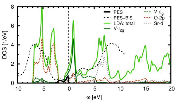
Figure 1: (Color online) Density of states within LDA in comparison with experimental spectra: PESSekiyama et al. (2004) and PES+BISMorikawa et al. (1995).

Figure 1 summarizes the Kohn-Sham electronic structure of density functional theory within the local density approximation (LDA): the O-2p states disperse between -2 and -7 eV, separated from the t_2g states whose bandwidth extends from -1 eV to 1.5 eV. While the t_2g and e_g bands are well separated at every given k-point, the partial density of states (DOS) slightly overlap, and the e_g states display a pronounced peak at 2.3 eV. Finally, peaks stemming from the Sr-d states are located at 6.1 eV and 7.1 eV. We have superimposed to the LDA DOS the experimental PES and Bremsstrahl-Isochromat spectroscopy (BIS) curves taken from Refs. Sekiyama et al., 2004; Morikawa et al., 1995. The comparison reveals the main effects of electronic correlation in this material: as expected on quite general grounds, LDA locates the filled O-2p states at too high and the empty Sr-d manifold at too low energies. The t_2g manifold undergoes a strong quasi-particle renormalization with a concomitant shift of spectral weight, both of which are effects beyond the one-particle picture. Photoemission studies Fujimori et al. (1992) early on provided detailed information on the disagreement between the measured spectra and the LDA DOS: In the experimental spectra the t_2g spectral weight extends down to binding energies of about -2eV, i.e. to 1eV lower than is found in LDA. On the basis of comparison with the Mott insulating compound YTiO₃ the observed additional peak between -1.5 eV and -2 eV was identified as a lower Hubbard band (LHB) – due to the removal process of an electron from an atomic-like localized t_2g state – , whereas the low-energy spectral weight was attributed to renormalized but coherent band states. A BIS study located an electron addition peak at energies around 2.7 eV Morikawa et al. (1995).

With the advent of dynamical mean field theory, explicit calculations for spectra for an infinite-dimensional Hubbard model became available Georges et al. (1996), supporting the idea of Hubbard bands persisting in the metallic state. The qualitative resemblance of the photoemission spectra with the occupied part of the three-peak structure of the infinite-dimensional one-band Hubbard model suggested SrVO₃ to be a prototypical correlated metal, in which the coexistence of quasi-particle states and Hubbard bands as well as their dispersions could be studied. Due to the high symmetry of the crystal structure, and the resulting threefold degeneracy of the t_2g bands, it was moreover argued that a purely local self-energy would lead to “pinning” of the value of the fully interacting spectral function at the Fermi level to the one corresponding to the density of states of the one-particle band structure. Any deviation from such “pinning” behaviorMüller-Hartmann (1989) can thus be taken as a proxy for nonlocal components in the many-body self-energy Morikawa et al. (1995).

A difficulty arose from the extreme surface sensitivity of the photoemission process, as evidenced in Refs. Inoue, 1998; Inoue et al., 1998; Maiti et al., 2001, 2006. These authors performed systematic photoemission studies at different photon energies, and witnessed a pronounced photon energy dependence of the quasi-particle peak, which they rationalized as a varying surface sensitivity. Measurements at high photon energies (900 eV) Sekiyama et al. (2004) indeed found a more developed $t_{2g}$ quasi-particle peak, in agreement with upcoming many-body calculations within dynamical mean field theory using the LDA density of states (DOS) or the LDA Hamiltonian as input Nekrasov et al. (2005); Liebsch (2003); Pavarini et al. (2004, 2005). The increased intensity ratio of the quasi-particle and satellite feature thus suggested nonlocal self-energy effects, neglected in DMFT, to be small. Interestingly, even the surface sensitivity could be modelled within such calculations Ishida et al. (2006). Angle-resolved photoemission spectra Yoshida et al. (2005) measuring the Fermi surface of SrVO₃ found cylindrical Fermi sheets, in agreement with theory, confirming the picture of a normal Fermi liquid.

Subsequent ARPES work adopted different strategies to increase bulk sensitivity: Laser ARPES Eguchi et al. (2006) studied the very low-energy spectral features, finding a “dip” at the Fermi level or a maximum of the quasi-particle peak slightly below (at around -0.2 eV). This work reopened the question about the role of nonlocal self-energy effects in the very low-energy properties of SrVO₃, since it remained unclear whether this feature is a result of the different experimental conditions of the laser ARPES setup (restricted Brillouin zone sampling, matrix elements or other), or whether it reflects the true bulk electronic structure at these very low energies. For a half-filled one-band Hubbard model on a cubic lattice, a similar “dip” effect was indeed found within a cluster dynamical mean field study Zhang and Imada (2007). Very recently, a realistic dynamical cluster approximation study Lee et al. (2012) confirmed the possibility of nonlocal effects inducing such a depletion at the Fermi level.

Takizawa et al. used thin films with atomically flat surfaces prepared in situ Takizawa et al. (2009), and were able to observe the band dispersions not only of the coherent band but also of the Hubbard bands. An interesting effect was observed concerning the lower Hubbard band: its intensity is strongly momentum-dependent, with its maximum in regions where also the band states are occupied (k$<$ k_F), whereas they fade away for k-points corresponding to empty coherent bands Yoshida et al. (2010), in agreement with theoretical modeling within DMFT Takizawa et al. (2009). Recently, also SrVO₃-based hetero-structures have been studied experimentallyYoshimatsu et al. (2010) and suggested for electronic device applicationsZhong et al. (2013).

The overall picture which emerges from all these works is that of a correlated metal with a quasiparticle mass enhancement of about 2 Morikawa et al. (1995); Maiti et al. (2006); Sekiyama et al. (2004); Takizawa et al. (2009); Aizaki et al. (2012) and a photoemission (Hubbard–)satellite at around -1.6 eV binding energy. This physics is reproduced by dynamical mean field calculations using the LDA electronic structure as input. The first works Nekrasov et al. (2005); Liebsch (2003); Pavarini et al. (2004, 2005) used a low-energy model comprising only the t_2g manifold, where the local orbitals are constructed from a downfolding procedure that incorporates also the ligand O-2p tails. Different choices of such orbitals were compared Lechermann et al. (2006), demonstrating that as long as the considered energy window is restricted to the t_2g bands only, results do not depend on the precise choice of the local orbitals (maximally localized Wannier functions, Nth order muffin tin orbitals, or projected atomic orbitals).

SrVO₃ became the drosophila of combined LDA and DMFT calculations, and new implementations were quite systematically tested on this compound (see e.g. Lechermann et al. (2006); Trimarchi et al. (2008); Amadon et al. (2008); Aichhorn et al. (2009); Karolak et al. (2011)). Apart from the effective t_2g model, also Hamiltonians including explicitly V-d and O-2p ligand states in the non-interacting Hamiltonian were used Amadon et al. (2008); Aichhorn et al. (2009); Karolak et al. (2011). It has been argued that the inclusion of ligand states leads to more localized d-orbitals, and an a priori better justification of the local approximation made by DMFT.

Momentum-resolved spectral functions were calculated from dynamical mean field theory in Ref. Nekrasov et al., 2006, in agreement with the experimental dispersion. They evidenced an additional feature, a “kink” structure at around -0.3 eV binding energy, which was later on rationalized as a generally expected phenomenon in correlated electron materials Byczuk et al. (2007): of purely electronic origin, kinks appear at the crossover scale at which the low-energy linear (Fermi liquid) behavior of the real part and the quadratic behavior of the imaginary part of the self-energy cease to be valid. In the meanwhile, kink structures observed in other materials, e.g. LaNiO₃ Eguchi et al. (2009), were also investigated theoretically and have been consistently reproduced by dynamical mean field calculations Deng et al. (2012). For SrVO₃, the theoretical predictions stimulated an intense search in photoemission spectra. While Ref. Takizawa et al., 2009 still had to conclude that “the kink is weak and broad, if it exists, but the curvature does indeed change sign at around -0.2eV, as predicted”, the very recent work by Aizaki et al. indeed identified such a kink structure at around -0.3 eV Aizaki et al. (2012).

Besides dynamical mean field theory and extensions, also other techniques of many-body theory were employed to investigate SrVO₃. A Gutzwiller study Deng et al. (2009) investigated the mass renormalizations, and renormalized densities of states as a function of the Hubbard $U$. Interestingly, to obtain the experimentally observed mass enhancement a $U$ value beyond 5 eV was found to be necessary in this scheme. Cluster model calculations systematically addressed the spectroscopic properties of SrVO₃ and analyzed the necessary ingredients for a minimal model thereof Mossanek et al. (2006, 2009, 2008); Wadati et al. (2009). These studies emphasized the strong pd-hybridization, which is responsible for the large charge transfer energy $\epsilon_{d}-\epsilon_{p}$. Interestingly, an analysis of the orbital character of the different spectral contributions identifies the spectral weight corresponding to the t_2g addition process as lying mainly between the Fermi level and about 1 eV, in contradiction with the dynamical mean field studies which suggest an upper Hubbard band of t_2g character at around 2.7 eV, that is at the precise location of the pronounced peak in BIS spectra. The cluster model calculation attributed this latter peak to the electron addition into e_g states Mossanek et al. (2009). We will come back to this point below.

With the advent of the constrained random phase approximation (cRPA) Aryasetiawan et al. (2004a) it became possible to calculate the values of the local Coulomb interactions (“Hubbard U”) specifically for the model under consideration. Again, SrVO₃ was chosen as a test material to demonstrate the power of the method Aryasetiawan et al. (2006); Miyake and Aryasetiawan (2008a), and it was shown that while U values for a full model comprising ligand states as well as V-d states can be as large as 8 eV for the d-orbitals, for a t_2g-only model the obtained value was quite small: 3.5 eV. The $U$ values used in the above cited LDA+DMFT calculations, on the other hand, varied rather between 4 eV and 5.5 eV. These values were such as to reproduce the observed mass enhancement, even though the position of the lower Hubbard band (LHB) was generally at slightly too high binding energies, suggesting that these values of $U$ were indeed on the large side. LDA+DMFT calculations with a $U$ value of 3.5 eV, however, do not reproduce the observed mass enhancement, nor result in a clear LHB. This puzzle was solved only recently Casula et al. (2012b): it was pointed out that $U$ should be considered as a dynamical quantity rather than a static interaction Aryasetiawan et al. (2004a, 2006). An LDA+$\mathcal{U}(\omega)$+DMFT calculation taking not only the ab initio value of the static component of $U=3.5$ eV but also its full frequency dependence into account indeed reproduced the observed mass enhancement as well as the position of the lower Hubbard band Casula et al. (2012b). This effect has very recently been confirmed within an analogous study, using a different impurity solver scheme Huang and Wang (2012).

In the following, we briefly emphasize a few puzzles, that remain within the dynamical mean field description of SrVO₃, resulting from the above mentioned works.

• Inconsistency between LDA+DMFT and cluster model calculations in the unoccupied part of the spectra
  While the assignment of orbital character to the peaks in the spectral function made by the cluster model calculations Mossanek et al. (2009) coincides in the occupied part of the spectra with the results of dynamical mean field theory (or, to account also for the correct position of the LHB, of LDA+$\mathcal{U}(\omega)$+DMFT), the position of the upper Hubbard band (UHB) at 2.7 eV found within the LDA+DMFT literature is inconsistent with the cluster model findings.

• Interpretation of 2.7 eV BIS feature as an upper Hubbard band inconsistent with ab initio $U$ values
  The interpretation of the BIS peak at 2.7 eV as an UHB of t_2g character, done in the LDA+DMFT literature, is inconsistent with the static value of $U$ from cRPA. Indeed, from the position of the LHB ($\sim$ -1.5 ev) and the static $U$ value (3.5eV) one would expect an UHB at 2 eV (as found in the LDA+$\mathcal{U}(\omega)$+DMFT calculation Casula et al. (2012b)). This leaves the photoemission feature at 2.7 eV unexplained within LDA+DMFT.

• Position of O2p ligand states
  LDA+DMFT calculations that also include oxygen ligand orbitals, do not in principle account for corrections to the LDA for these orbitals. Such corrections have been introduced by hand as an arbitrary shift on the O2p states Amadon et al. (2008); Aichhorn et al. (2009). This means that this position is not known ab initio from LDA+DMFT. On the other hand, it is well-known that in the related compound SrTiO₃, which is isostructural to SrVO₃ but of d⁰ configuration, the pd-gap of Kohn-Sham theory within the LDA is underestimated by 1.3 eV compared to experiment van Benthem et al. (2001).

• Position of Sr-4d states
  An analogous problem arises when comparing the energetic position of the Sr-4d states in BIS and in Kohn-Sham density functional theory, which underestimates their energy by almost 2 eV. By construction, combined LDA+DMFT schemes do not correct for this error.

• Relation between laser ARPES results and nonlocal effects
  To the best of our knowledge, it remains open at this stage how to reconcile the laser ARPES experiments (and in particular the finding of a dip at the Fermi level) with the high-photon energy PES which display a pronounced peak. The study of nonlocal many-body effects on a very low-energy scale remains thus a challenging task for the future.

The present work addresses the first four issues, leaving the last one for future work. In particular, we review and extend the GW+DMFT calculations of Ref. Tomczak et al., 2012b. Since the publication of Ref. Tomczak et al., 2012b electronic structure calculations for SrVO₃ have met renewed interest: besides a study Gatti and Guzzo (2013) within the GW approximation (including a cumulant correction similar to the above discussed Bose factor ansatz), several groups have embarked into attempts of setting up simplified schemes mimicking the results of GW+DMFT. Interestingly, while different elements of the full calculations are indeed captured in the different schemes, no scheme so far could fully reproduce the low-energy behavior, and the question of designing approximate schemes in a specific low-energy range remains a largely open one. We will therefore also devote an extended paragraph to a systematic comparison of different approximate schemes and a discussion of what they can be expected to provide.

IV Results

We now turn to the description of the results of GW+DMFT calculations using the formalism outlined above for our target compound, SrVO₃. The GW+DMFT calculations will be put into perspective by confronting them to pure GW calculations, as well as to LDA+DMFT calculations both, with static and dynamical interactions. As a prelude, we discuss the dynamical Hubbard interactions obtained for SrVO₃ within the cRPA scheme.

IV.1 Dynamical interactions

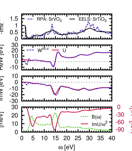
Figure 2: (Color online) Dynamical screening in SrVO₃. From top to bottom: (a) comparison of the inverse dielectric function of SrVO₃ within RPA with the experimental EELS spectrum of SrTiO₃Kohiki et al. (2000). (b)/(c) real/imaginary par of the fully (partially) screened interaction $W^{loc,d}$ ($\mathcal{U}$) in the Wannier basis. (d) Bosonic factor (see text for definition) and density of screening modes $\mathrm{Im}\ \mathcal{U}(\omega)/\omega^{2}$.

In Figure 2, we plot the screened and partially screened Coulomb interactions: $W$ denotes the matrix element of the fully screened interaction in t_2g maximally localized Wannier functions and the Hubbard $\mathcal{U}$ is defined in Eq. (27).

The physical interpretation of the frequency-dependence of the interactions is transparent, if one recalls that the effective bare interaction within a subspace of the original Hilbert space should include screening by the omitted (e.g. higher-energy- Aryasetiawan et al. (2004a) or nonlocal-Nomura et al. (2012)) degrees of freedom. Indeed, the net result of the rearrangement of the high-energy degrees of freedom as response to a perturbation of the system is an effective reduction of the perturbation strength in the low-energy space. The effective Coulomb interaction in a low-energy effective model for a correlated system is therefore in general an order of magnitude smaller than the matrix element of the bare Coulomb interaction. Nevertheless, the latter is recovered in the limit of high-frequencies of the perturbation, when screening becomes inefficient. The crossover – as a function of frequency – from the low-energy screened regime to the high-frequency bare matrix element of $\frac{e^{2}}{|{\bf r}-{\bf r}^{\prime}|}$ takes place at a characteristic screening (plasma) frequency where the dielectric function exhibits a pole structure.

For SrVO₃, the (partially) screened interaction, corresponding to the dynamical Hubbard interaction at vanishing frequency, takes on a value of $U=3.5$ eVMiyake and Aryasetiawan (2008a) for the t_2g orbital-subspace spanned by maximally localized Wannier functions. The corresponding Hund’s rule exchange $J$ is 0.6 eV. The bare interaction, the matrix element of the Coulomb interaction within the t_2g Wannier orbitals, equals $V=15$ eV. As seen in Fig. 2, the crossover from the low-energy screened regime to the high-energy tail takes place at about 15 eV. At this energy, a well-defined plasma excitation is observed. Indeed, the upper panel reproduces experimental electron energy loss (EELS) spectra for the related compound SrTiO₃Kohiki et al. (2000). This material is isostructural to our target compound, and has one electron less (d⁰ configuration). The EELS data display a well-defined plasmon excitation at about 15 eV. The experimental spectrum is well-reproduced by the theoretical imaginary part of the inverse dielectric function calculated within the RPA. The reason that, besides higher energy one-particle derived features, also the collective plasmon satellite of $d^{0}$ SrTiO₃ is well described by our calculation for the non-isoelectronic $d^{1}$ SrVO₃ resides in the fact that it is not dominated by d-electron contributions. This is evident since the fully and partially screened interaction of the $t_{2g}$ orbitals, $W_{t2g}$ and $U_{t2g}$, are very similar at these energies. Overall, this validates using the LDA electronic structure for the purpose of calculating the effective interaction $\mathcal{U}(\omega)$ of SrVO₃.

The fully screened interaction $W$ furthermore exhibits a weaker feature at low energies ($\sim$ 2 eV), a “subplasmon”, corresponding to a collective charge oscillation of the t_2g charge only. This peak is therefore not present when the t_2g screening processes are cut out, as is the case in the construction of the effective interaction $\mathcal{U}(\omega)$. As we will see later, this is the energy regime where the local vertex corrections introduced by DMFT modify the GW description of the spectral properties. Features at these energies produced within GW calculations are thus not present any more in the GW+DMFT results (see below).

In the many-body calculation, the frequency-dependent interaction enters the bosonic factor $B(\tau)$ of Eq. (37) in the form of $\mathrm{Im}\ \mathcal{U}(\omega)/\omega^{2}$. This function can be interpreted as the density of screening modes. It is plotted in the lowest panel of Fig. (2), together with the spectral function of $B(\tau)$ defined in Eq. (36). Interestingly, these functions allow to identify yet another feature, namely a well-defined peak at about 5 eV. We will come back to this point later.

IV.2 GW

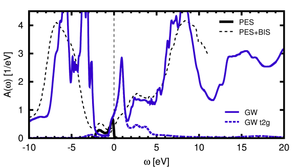
Figure 3: (Color online) The GW spectral function in comparison to the same experiments as in Fig. 1.

Several of the deficiencies of DFT calculations mentioned above can be addressed with Hedin’s GW approximationHedin (1965), that uses the fully screened interaction $W$ discussed in the previous section. We will in particular address the following two issues:

1. higher energy states (O2p, Sr4d, …). Improvement of these is governed by exchange and correlation effects (beyond DFT) that (i) lie outside the realm of purely local interactions, and (ii) are beyond the (low energy / t_2g) orbital subspace. Thus inaccessible to DMFT-based methods, their correction is one pivotal merit that GW contributes to theories beyond DFT and DFT+DMFT.

2. many-body effects at low energies. Here we will discuss the impact of many-body renormalization on the t_2g spectrum, with particular focus on nonlocal self-energy effects (beyond DFT, and absent in DMFT).

Besides a better description of the electronic structure of SrVO₃, our GW calculation also gives useful fundamental insights into the nature of correlation effects in transition metal oxides. We will present evidence that dynamical and nonlocal correlation effects can essentially be separated (this was previously discovered for the iron pnictides and chalcogenides in Ref. Tomczak et al., 2012c). Further we will discuss the spatial extent of correlation effects in real space, putting into perspective corrections to the local picture of DMFT.

IV.2.1 Correction of higher energy features

The GW spectral function is shown in Fig. 3. In the unoccupied part of the spectrum a substantial improvement over the LDA band-structure result, Fig. 1, is seen: states beyond the t_2gs are in excellent agreement with inverse photoemission results. In particular the hump at around 2-5eV is very well captured. In contrast to assignments in the DMFT literature, its spectral weight stems largely from the vanadium $e_{g}$ states within GW, in congruence with cluster based methods.Mossanek et al. (2009) Beyond 5eV appear the Sr4d orbitals, again in remarkable accordance with the experimental intensity.

Also the position of occupied states, the O2p orbitals in the shown energy range, improve to the extent that the experimental satellite at -1.6eV is no longer obscured by oxygen spectral weight. With respect to the photoemission experiment however, the binding energy of the O2p is still too small by at least an electronvolt. A possible remedy to this issue could be to extend the Wannier space to the O2p and vanadium $e_{g}$ states and include a local Hubbard interaction on the latter in the GW+DMFT. This would favour a charge transfer into the O2p orbitals with which the $e_{g}$ states hybridize most, thus pushing the oxygen states further down. In our GW+DMFT calculations here, we only consider the impact of local Hubbard interactions on the $t_{2g}$ subspace.

IV.2.2 Low energy renormalizations

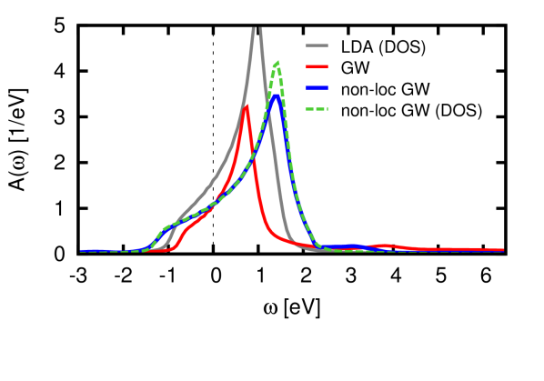
Figure 4: (Color online) Comparison of the local GW spectral function with the LDA density of states. Also shown is the spectral function and density of states of nonlocal-GW. See text for details.

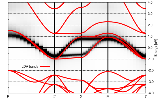
Figure 5: (Color online) Momentum resolved spectral function (a) within the GW approximation and (b) taking into account only the nonlocal part of the GW self-energy. Superimposed is the LDA band structure.

Also shown in Fig. 3 is the $t_{2g}$ contribution to the full spectral function. The t_2g bandwidth is reduced by about 25% with respect to LDA, see also the momentum resolved spectra in Fig. 5 and Fig. 10. This suggests an overall effective mass $m_{\hbox{\tiny{\it GW}}}/m_{\hbox{\tiny LDA}}\sim 1.3$. The corresponding spectral weight is transferred to satellites that correspond to the features seen in the fully screened interaction $W$, see Fig. 2, namely at $\pm(\sim 2)$eV as well as the $t_{2g}$ contributions to the plasmon satellite at 17eV.

To analyze the low-energy renormalizations further, we note that the mass enhancement relative to the LDA band masses is given by the ratio of the magnitudes of the group velocities within LDA, $\frac{d\epsilon_{{\mathbf{k}}i}}{dk_{\alpha}}=\langle\Psi_{{\mathbf{k}}i}|\partial_{k_{\alpha}}{H_{\hbox{\tiny{\hbox{\tiny LDA}}}}}({\mathbf{k}})|\Psi_{{\mathbf{k}}i}\rangle_{k=k_{F}}$, and the GW

$$\frac{dE_{{\mathbf{k}}i}}{dk_{\alpha}}=\left.\frac{\langle\Psi_{{\mathbf{k}}i}|\partial_{k_{\alpha}}\left(H_{\hbox{\tiny{\it LDA}}}({\mathbf{k}})+\mathrm{Re}\Sigma_{\hbox{\tiny{\it GW}}}({\mathbf{k}},\omega)\right)|\Psi_{{\mathbf{k}}i}\rangle}{\left(1-\langle\Psi_{{\mathbf{k}}i}|\partial_{\omega}\mathrm{Re}\Sigma_{\hbox{\tiny{\it GW}}}({\mathbf{k}},\omega)|\Psi_{{\mathbf{k}}i}\rangle\right)}\right|_{k=k_{F},\omega=0},$$ (39)

evaluated on the Fermi surface. Here, the self-energy is defined with respect to the LDA exchange-correlation potential: $\Sigma_{\hbox{\tiny{\it GW}}}=\Sigma^{xc}_{\hbox{\tiny{\it GW}}}-v^{xc}_{\hbox{\tiny LDA}}$. Thus (besides a modified electron density), two ingredients for changes in effective many-body masses can be identified: (a) the dynamical part of the self-energy through the quasi particle weight $Z_{\mathbf{k}}=1/\left(1-\partial_{\omega}\mathrm{Re}\Sigma_{\hbox{\tiny{\it GW}}}({\mathbf{k}},\omega)\right)_{\omega=0}$, and (b) a renormalization via the nonlocality of the self-energy, $\partial_{k_{\alpha}}\mathrm{Re}\Sigma({\mathbf{k}},\omega)$. In DMFT-based approaches, where the self-energy is local by construction, only the first mechanism is present, hence $m_{\hbox{\tiny DMFT}}/m_{\hbox{\tiny LDA}}=1/Z_{\hbox{\tiny DMFT}}$.

The weight of the t_2g quasi-particles in SrVO₃ is $Z_{k_{F}}\sim 0.53$ within the GW approximation. This is virtually the same value that is found for the homogeneous electron gas at the same density, $r_{s}=7.26$, when using the same methodHedin (1965). The low quasi-particle weight in conjunction with the only moderate bandwidth narrowing, $m_{\hbox{\tiny{\it GW}}}/m_{\hbox{\tiny LDA}}=1.3$, thus advocates a notable enhancement of the group velocity, and thus band-width, from nonlocal correlations. We find it instructive to compute the spectral function when only taking into account these nonlocal effects. To this effect, we take out the local part of the GW correlation self-energy and construct $\Sigma_{GW}^{non-loc}(k,\omega)=\Sigma^{xc}_{GW}(k,\omega)-\left(\Sigma^{c\ loc}(\omega)-\Sigma^{c\ loc}(\omega=0)\right)-v^{xc}(k)$, where $\Sigma^{c\ loc}=\sum_{k}\Sigma^{c}_{GW}$. The spectral function of this “nonlocal-GW” is shown in Fig. 5(b) for a selected k-path, while the local projection can be seen in Fig. 4. As anticipated, the t_2g bandwidth is substantially widened. It becomes 44% larger than the dispersion of the LDA. In particular we see that this effect is notably more pronounced in the unoccupied part of the spectrum. DFT being a theory to yield the correct ground state properties (if the exact $v^{xc}$ was known), it seems natural that occupied states are better captured than unoccupied (excited) states (even though of course, the Kohn-Sham spectrum in principle has no physical meaning to begin with). Also shown in Fig. 4 is the nonlocal-GW density of states, in which all (local and nonlocal) imaginary parts of the GW self-energy are omitted. The presence of nonlocal correlation effects in the GW approximation for SrVO₃ can also be evidenced as follows: Indeed, for a purely local self-energy, and in the absence of orbital charge transfers (the t_2g-orbitals are locally degenerate), the value of the spectral function at the Fermi level, $A(\omega=0$), is “pinned” to its non-interacting (LDA) valueMüller-Hartmann (1989). The violation of this pinning condition, see Fig. 4, is thus heralding a nonlocal self-energy. Obviously, the evidenced nonlocal renormalization is also beyond DFT+DMFT approaches, and hence another crucial contribution of the GW to schemes such as GW+DMFT.

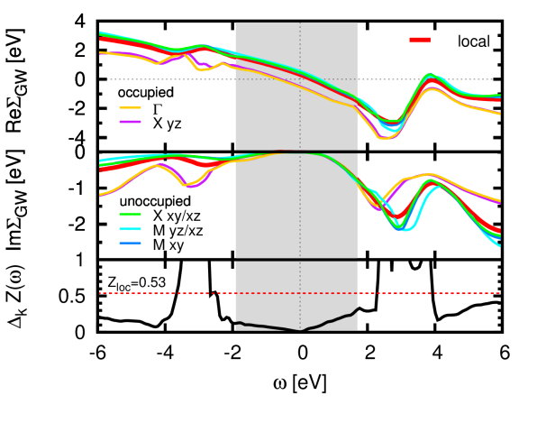
Figure 6: (Color online) The GW self-energy at several high symmetry points resolved into the three t_2g (Wannier) orbitals as a function of frequency. Also shown is the local projection (real parts: top panel, imaginary parts: middle panel). The lower panel displays the momentum variance of the frequency dependent generalization of the quasi-particle weight. The origin of energy corresponds to the Fermi level and the shaded area roughly delimits the Fermi liquid regime within GW.

Thus, the fact that the LDA and full (local + nonlocal self-energy) GW dispersion are somewhat comparable is owing to the competition of a band-width narrowing through the dynamics of the self-energy, and the tendency of nonlocal contributions to delocalize charge carriers. However, the physics underlying these similar dispersions is very different: Indeed within the GW, almost half of the t_2g spectral weight is transferred to collective excitations at higher energies. This phenomenon is absent in effective one-particle theories such as DFT, but a physical reality, see e.g. the EELS data in the preceding section. However, due to the perturbative nature of GW, and its limitations regarding dynamical local correlationsTomczak et al. (2012c), it is not able to reproduce the lower Hubbard satellite seen in photoemission spectroscopy (Fig. 3).

IV.2.3 Separability of dynamical and nonlocal correlations

Having discussed different ingredients to band-width renormalizations, we now examine the nature of correlation effects in more detail.

For the case of the iron pnictides and chalcogenides, Tomczak et al. Tomczak et al. (2012c) found that – within the GW approximation – electronic correlation effects in the Fermi liquid regime are separable into a dynamical self-energy that is local, and nonlocal contributions that are static. This notion of locality holds when the self-energy is expressed in a local basis, in our case the maximally localized Wannier functions for the t_2g subspace. Does this empirical finding extend to the transition metal oxide SrVO₃? In the upper panel of Fig. 6 the real part of the GW self-energy of SrVO₃ is shown for several high symmetry points in the Brillouin zone as well as the local, i.e. momentum summed, element, as a function of frequency. The offset, $\Sigma_{\hbox{\tiny\it GW}}(\omega=0)$, is positive for unoccupied orbital characters (xy/xz at the X point, and all t_2g’s at the M point, cf. Fig. 10), and negative for the occupied orbitals. Thus (un)occupied spectral weight gets pushed (up) down in energy, congruent with the changes in the bandwidth seen in Fig. 4 and Fig. 5(b), as well as the reduction of the effective mass from the value of the inverse quasi-particle weight $1/Z$.

Regarding the frequency dependence, one can see that the self-energy is linear from roughly -2 to +1.8eV, which thus delimits the Fermi liquid regime within the GW approximation. The slope of the self-energy is slightly larger for $\omega>0$, thus compensating, in part, the static shift that is larger for unoccupied states. Correspondingly, the imaginary part of the self-energy also grows faster with frequency in the unoccupied part, signalling stronger correlations for $\omega>0$. The important finding here is that in the Fermi liquid regime, the frequency dependence (the linear slope in the real parts) at different momenta are very similar. That is to say that dynamical renormalizations in different regions of the Brillouin zone are comparable. To investigate this more quantitatively, we define

$$Z_{\mathbf{k}}(\omega)=\left[1-\frac{\partial\mathrm{Re}\Sigma({\mathbf{k}},\omega)}{\partial\omega}\right]^{-1}$$ (40)

as a generalization of the quasi-particle weight $Z_{k_{F}}(\omega=0)$. We further introduce its momentum varianceTomczak et al. (2012c)

$$\Delta_{k}Z=\sqrt{\sum_{\mathbf{k}}Tr|Z_{{\mathbf{k}}}{(\omega)}-Z^{loc}(\omega)|^{2}}$$ (41)

as defined with respect to the local projection $Z^{loc}$ of Eq. 40, where the trace sums over the Wannier orbitals. Then, $\Delta_{k}Z$ is a measure for the importance of dynamical self-energy effects that are nonlocal. As is apparent from Fig. 6, $\Delta_{k}Z$ virtually vanishes at the Fermi level and is small compared to $Z^{loc}(\omega=0)=0.53$ within the linear regime.

This means that – at least at the GW level – the dynamics of the quasi-particle renormalization is local, and, conversely, that nonlocal correlation effects are static.Tomczak et al. (2012c) As a consequence, the self-energy becomes separable: The dynamical part is (almost) purely local, thus justifying the use of local but dynamic theories such as DMFT. The nonlocal part, on the other hand, is static, as in theories employing generalized (orbital and momentum dependent) effective potentials such quasi-particle self-consistent (QS)GWFaleev et al. (2004)^, .

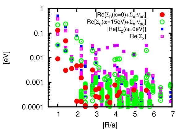
Figure 7: (Color online) The GW self-energy correction to DFT as a function of real space distance at the Fermi level ($\omega=0$) and the energy region of the plasmon satellite ($\omega=15$eV). The occurrence of several values per distance owes to different orbital orientations at growing numbers of neighbours. Also shown are the absolute values of the ($\omega=0$) correlation and exchange self-energies of the GW.

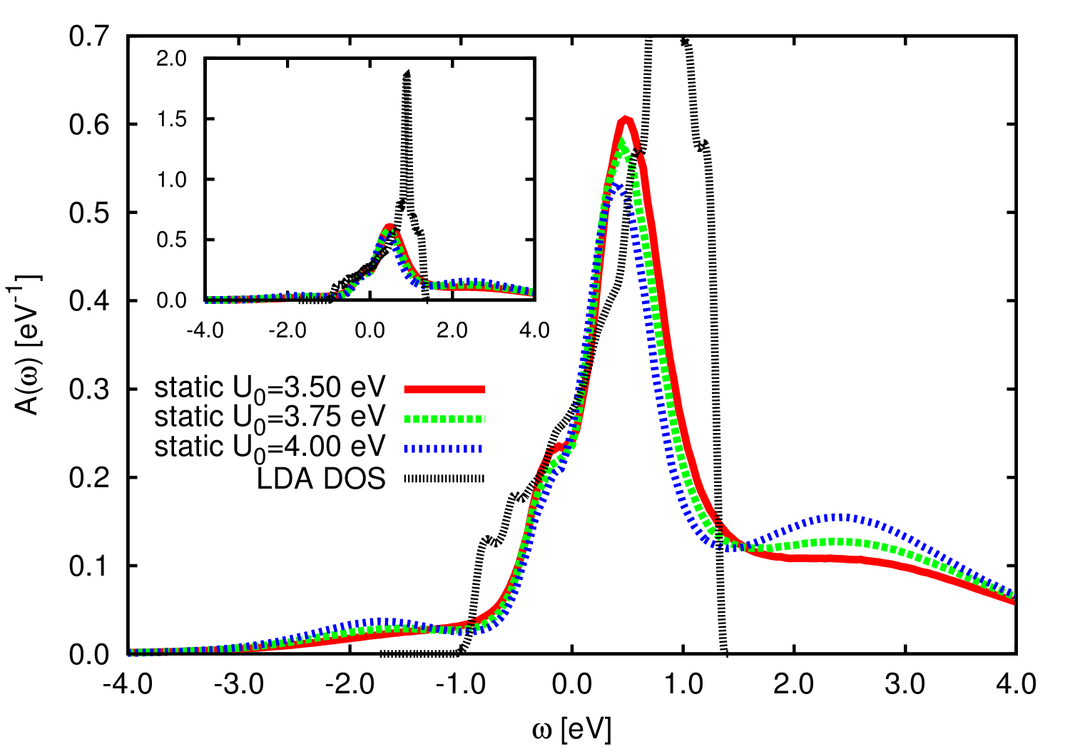
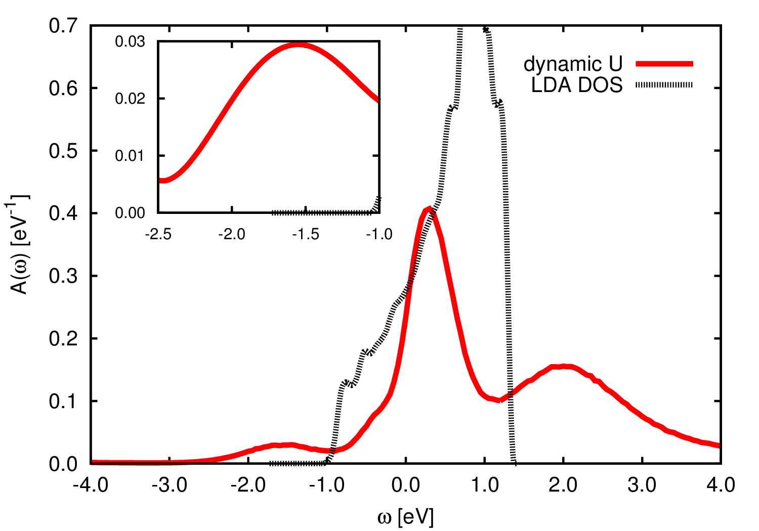
Figure 8: (Color online) Local spectral function from standard LDA+DMFT with static interactions (left). LDA+DMFT with dynamical interactions (right). Here, the spectral functions are normalized to one, such that the filling corresponding to SrVO₃ is 1/6.

This non-trivial finding suggests that for many materials (in and for their Fermi liquid regime) the separation into local and nonlocal self-energies à la GW+DMFT simplifies to the extent that nonlocal correlations can be accounted for by a nonlocal yet static potential. This led the authors of Ref. Tomczak et al., 2012c to propose a QSGW+DMFT scheme, in which the QSGW constructionFaleev et al. (2004) is used to provide that potential.

IV.2.4 Bandwidth widening by nonlocal self-energy contributions

We now discuss more in detail the widening of the band by nonlocal self-energy contributions, as seen in Fig. 5. To this effect, we note that the separation of the self-energy into a local dynamical and a nonlocal static part can be interpreted as a generalization of the familiar Coulomb-hole-screened exchange (COHSEX) approximation to a full GW treatment. Indeed, in the COHSEX approximation Hedin (1965) the GW self-energy is given by a static self-energy of the following form:

$$\Sigma(r,r^{\prime},\omega)=\Sigma_{SEX}(r,r^{\prime})+\Sigma_{COH}(r,r^{\prime})$$ (42)

where the first term is a screened exchange self-energy built from the static screened Coulomb interaction

$$\Sigma_{SEX}(r,r^{\prime})=-\sum_{kn}^{occ}\phi_{kn}(r)\phi^{\ast}_{kn}(r^{\prime})W(r,r^{\prime},\omega=0)$$ (43)

and the second contains the effect of the Coulomb hole

$$\Sigma_{COH}(r,r^{\prime})=\frac{1}{2}\delta(r-r^{\prime})(W(r,r^{\prime},\omega=0)-v(r-r^{\prime}))$$ (44)

Here, the indices $k,n$ denote Kohn-Sham states of wave vector $k$, and the sum runs over occupied states only. Interestingly, when separating the COHSEX self-energy into local and nonlocal parts in the many-body sense (that is, with respect to a localized basis set), the nonlocal contribution stems from the screened exchange self-energy only. For a system such as SrVO₃, the local part of $\Sigma_{SEX}$ is – by symmetry – a scalar in the space of t_2g-orbitals, and can thus be considered an irrelevant constant in that space. The Coulomb hole self-energy, on the other hand, is purely local.

The separation in static nonlocal and dynamical local parts found in the preceding section can therefore be interpreted in the following way:
(1) The nonlocal contribution to the self-energy can be interpreted as a screened exchange self-energy $\Sigma_{SEX}=GW(\omega=0)-[GW(\omega=0)]_{local}$.
(2) The local contribution contains the Coulomb hole effect as well as band renormalizations beyond the COHSEX approximation, stemming from the frequency-dependence of the local dynamical self-energy.

Therefore, when considering the band structure corresponding to the nonlocal self-energy contribution only, the Coulomb hole part as well as the dynamical correlations are taken out since they are purely local, and the remaining correction can thus be interpreted as the screened exchange contribution. The widening of the band as compared to the Kohn-Sham band structure is therefore the familiar broadening by exchange interactions (which, here, are screened, thus leading to substantial but not as large effects as in unscreened Hartree Fock theory).

The screened exchange self-energy correction to the DFT exchange correlation potential can be written as:

$$(\Sigma_{SEX}-v_{xc})(r,r^{\prime}) = -\sum^{occ}_{k^{\prime}n^{\prime}}\psi^{\ast}_{k^{\prime}n^{\prime}}(r)\psi_{k^{\prime}n^{\prime}}(r^{\prime})$$

$$\times \left(W(r,r^{\prime},\omega=0)-\delta(r-r^{\prime})\tilde{v}(r)\right)$$

with a potential $\tilde{v}(r)$ representing the Kohn-Sham exchange-correlation contribution.

Matrix elements of this quantity in the Kohn-Sham basis read

$$\langle k_{0}n_{0}|\Sigma_{SEX}-v_{xc}|k_{0}n_{0}\rangle$$ (46)

$$= -\sum^{occ}_{k^{\prime}n^{\prime}}\int d^{3}r\int d^{3}r^{\prime}\psi^{\ast}_{k^{\prime}n^{\prime}}(r)\psi_{k^{\prime}n^{\prime}}(r^{\prime})W(r,r^{\prime},\omega=0)$$

$$\times\psi^{\ast}_{k_{0}n_{0}}(r)\psi_{k_{0}n_{0}}(r^{\prime})+\int d^{3}r\tilde{v}(r)n(r)|\psi_{k_{0}n_{0}}(r)|^{2}$$

An intuitive inspection of these matrix elements suggests the resulting correction to be small for occupied $|k_{0}n_{0}\rangle$ states, but to result in an upward shift for unoccupied states. Indeed, for unoccupied states, the matrix elements $\langle k_{0}n_{0}k^{\prime}n^{\prime}|W|k_{0}n_{0}k^{\prime}n^{\prime}\rangle$ are necessarily between product states that mix occupied $|k_{0}n_{0}\rangle$ and unoccupied states $|k^{\prime}n^{\prime}\rangle$, and thus small compared to $V_{xc}$. This results in the familiar effect of a GW correction to conduction band states in simple semiconductors, leading to a “scissors” correction to the too small Kohn-Sham band gaps.

In the case of the metallic SrVO₃ with d¹ filling, the band widening by nonlocal contributions is much stronger for the unoccupied part of the spectrum (which is enhanced by more than 1 eV) than for the occupied part. As we will see below, this effect will carry through the GW+DMFT treatment, where the screened exchange band structure becomes renormalized by local dynamical correlations encoded in the DMFT self-energy.

IV.2.5 The spatial range of correlations

Having established the importance of nonlocal correlation effects, as well as their static nature at low energies, we want to characterize their extent in real space. Indeed there are efforts to extend DMFT calculations from the single impurity setup to a cluster of several sites (or several momenta) even for ab initio calculations. For the case of SrVO₃ this was first done in Ref. Lee et al., 2012 using the dynamical cluster approximation (DCA) method, that partitions the Brillouin zone into momentum patches (two patches, in the cited work) and thus gives momentum resolved information on a coarse grid.

Here, we will rather follow the spirit of cellular DMFT, in which real-space clusters are embedded into the solid, thus allowing nonlocal correlations of the range of the cluster size. The important question now is how big that cluster has to be in order to exhaust the extent of pertinent nonlocal correlations. For this we note that self-energy diagrams beyond GW give mainly local contributionsZein et al. (2006), and thus our findings based on the GW approximation are expected to have a wide range of validity.

In Fig. 7 we show the magnitudes of the GW self-energy corrections with respect to LDA at the Fermi level ($\omega=0$) and at energies near the plasmon peak ($\omega=15$eV) as a function of the real space distance to a reference vanadium atom.

At the Fermi level, this correction is indeed rather short-ranged: Already at the next-nearest (vanadium) neighbour it has decreased by one order of magnitude. This advocates that a 2x2x2 unit-cell cluster (beyond current computational capabilities) might already give meaningful results. In the region of the collective (plasmon) excitation, the decrease in magnitude occurs more slowly, suggesting much larger cluster sizes. This does not come as a surprise, since at these energies collective long-ranged excitations are dominant.

IV.3 DMFT

IV.3.1 DMFT with static interaction

SrVO₃ has been used as a benchmark compound for standard LDA+DMFT calculations, both within a low-energy description comprising only the t_2g states and including the oxygen ligands . It was argued that the static Hubbard interactions have to be at least as large as 4 eV to reproduce the experimentally observed mass enhancement. The local spectral function then displays a three-peak structure as in the correlated metal phase of the half-filled single-band Hubbard model, even though the low filling of 1 electron in 3 bands makes the spectra highly asymmetric. The lower Hubbard band, at $U$=4 eV, is located at slightly too low binding energy (nearly -2eV, instead of the experimentally observed -1.5 eV). At about 2.5 to 2.7 eV, an upper Hubbard band is found. Since this feature coincides in energy with an experimentally observed electron addition peak, the LDA+DMFT literature has thus identified the latter as an upper Hubbard band (see however the GW spectrum in Fig. 3 and the discussion below). When using the static component of the Hubbard interaction calculated within cRPA ($\sim$ 3.5 eV), however, a very weakly correlated metal is obtained, where the lower Hubbard band is barely a shoulder structure and the mass enhancement is much smaller than the experimentally observed one. Figure 8(a) reproduces the local spectral function for $U$ values varying between 3.5 eV and 4 eV, as calculated in Ref. Lechermann et al., 2006.

IV.3.2 DMFT with dynamical interaction

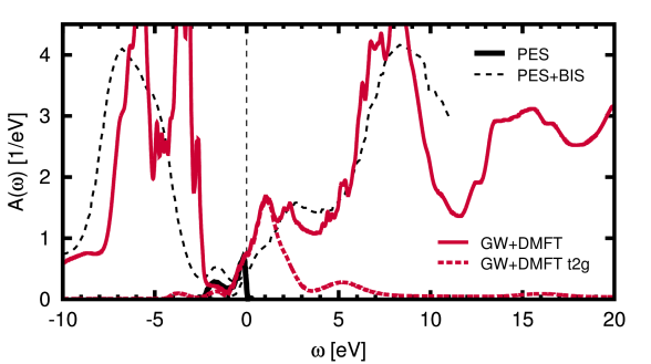
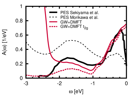
Figure 9: (Color online) GW+DMFT spectral function, in comparison to (inverse) photoemission spectra (same experiments as in Fig. 1).

The puzzle of the too weak mass renormalizations within LDA+DMFT when the static component of the cRPA $U$ is used was solved when it was realized that taking into account the frequency-dependence of the interactions leads to additional mass enhancements Casula et al. (2012b). Indeed, the high-energy tail of the dynamical interaction alone was shown to be at the origin of a mass enhancement of $Z_{B}^{-1}$ with $Z_{B}=0.7$ Casula et al. (2012b). The overall mass enhancement of the calculation with the dynamical cRPA interaction is $m^{*}/m_{\hbox{\tiny LDA}}\sim 2$, in reasonable agreement with ARPES estimates. Since, however, the static component of $U$ is smaller than what was used before in static LDA+DMFT calculations, the position of the lower Hubbard band is shifted towards the Fermi level, correcting the deficiency of LDA+DMFT discussed above. On the unoccupied side of the spectrum, an upper Hubbard band feature appears at about 2 eV, substantially lower than what was discussed within LDA+DMFT. Experimentally, such a feature is not clearly resolved. We can thus summarise the effect of dynamical interactions within LDA+$\mathcal{U}(\omega)$+DMFT calculations by noting that the only notable modification in the electronic structure is the improved description of the lower Hubbard band, compared to experiment, whereas the situation is less clear for the unoccupied part of the spectrum. We will argue below that this scheme is actually as little appropriate for unoccupied states as is the standard static LDA+DMFT.

IV.4 GW+DMFT

IV.4.1 Full calculations

We now discuss the results of our combined GW+DMFT calculations for the spectral properties of SrVO₃. Fig. 9(a,b) displays the local projection of the spectral function, while Fig. 10 shows momentum dependent t_2g spectra in comparison with ARPES measurementsTakizawa et al. (2009); Aizaki et al. (2012). The global view on the spectral function in the full energy range of valence and conduction band states, Fig. 9(a), reveals an overall remarkable agreement with experiments. Indeed, GW+DMFT inherits from the GW calculation the excellent agreement of the Sr-d states, both, in position and shape, with BIS spectra, and the improved agreement of the O-p ligand states with photoemission. The low-energy part of the spectrum is dominated by the t_2g contribution, which, here, is profoundly modified with respect to pure GW results. A renormalized quasi-particle band disperses around the Fermi level : At the $\Gamma$ point (see Fig. 10) the peak is located at about -0.5 eV – this reveals (in agreement with ARPES) a strong renormalization of the corresponding Kohn-Sham state which, at this momentum, has an energy of -1 eV. At the X-point, the t_2g bands are no longer degenerate, and surprisingly weakly renormalized xy/xz states are observed at 0.9 eV, while the yz band is located at nearly the same energy as at the $\Gamma$ point, again in agreement with ARPES. At binding energies of -1.6 eV, ARPES witnesses a weakly dispersive Hubbard band, whose intensity varies significantly as a function of momentum Takizawa et al. (2009). In the GW+DMFT spectral function the Hubbard band – absent in GW – is correctly observed at about -1.6 eV and its k-dependent intensity variation (see Fig. 10) is indeed quite strong. Previous LDA+DMFT calculations placed the lower Hubbard band at larger negative energies (see e.g. Pavarini et al. (2004)). This is owing to the fact discussed above that when using a static Hubbard interaction, a value of 4–6 eVPavarini et al. (2004); Amadon et al. (2008), that is larger than the zero frequency limit of the ab intio $\mathcal{U}(\omega$$=$$0)$$=$$3.5$eVMiyake and Aryasetiawan (2008b), is needed to account for the observed transfers of spectral weight. As in DMFT with dynamic $\mathcal{U}$, GW+DMFT yields a good description of the Hubbard band and the spectral weight reduction at the same time, thanks to the additional transfers of spectral weight due to the dynamical screening Casula et al. (2012b, a); Tomczak et al. (2012b).

At positive energies nonlocal self-energy effects are larger. Interestingly, our k-integrated spectral function, (see the dashed line in Fig.9(a) for the t_2g contribution to the total (solid line) spectrum) does not display a clearly separated Hubbard band. The reason is visible from the k-resolved spectra: the upper Hubbard band is located at around 2 eV, as expected from the location of the lower Hubbard band and the fact that their separation is roughly given by the zero-frequency value of $U$. The peak around 2.7 eV that appears in the inverse photoemission spectrum Morikawa et al. (1995) – commonly interpreted as the upper Hubbard band of t_2g character in the DMFT literature – arises in fact from e_g states located in this energy range. The nonlocal self-energy effects lead, in the unoccupied part of the spectrum, to overlapping features from different k-points and an overall smearing of the total spectral function.

The Bose factor ansatz discussed above does not only provide us with an efficient technique for solving the GW+DMFT equations. It also allows for a transparent physical interpretation of the arising spectral properties. Indeed the spectral representation of the bosonic renormalization factor $B(\tau)$ of Eq. 35 (displayed in the lower panel of Fig. 2) is directly related to the density of screening modes $\mathrm{Im}\ \mathcal{U}(\omega)/\omega^{2}$.Casula et al. (2012b) In this way, we can trace back the GW+DMFT satellite at -4.5 eV to the onset of p-t_2g excitations, discussed above for $W$ and $U$. On the other hand, since the feature below 3 eV in $W$ is absent in $U$ and $B$, the spurious GW peaks are consistently eliminated. The strong peak at 15 eV is the well-known plasma excitation, seen e.g. in electron energy loss spectra of SrTiO₃Kohiki et al. (2000).

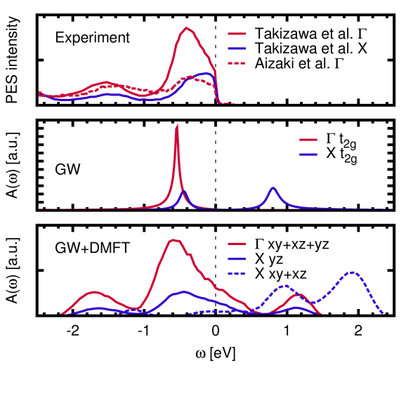
Figure 10: (Color online) Momentum-resolved spectral function from GW and GW+DMFT in comparison to photoemission experiments.

IV.4.2 Test of simplified schemes

We now turn to the question of how to set up simplified schemes that would still reproduce the results of the full GW+DMFT calculations within the low-energy regime. Besides the methodological interest, this study also allows us to analyse more in detail the dominant effects leading to corrections to the Kohn-Sham band structure.

As can be seen from the methodological section, the DMFT self-consistency condition for the one-body quantities requires the local Green’s function to equal

$$G^{loc}(i\omega)=$$

$$\sum_{k}[i\omega+\mu-H_{0}(k)-\Sigma_{GW}^{non-loc}(k,i\omega)-\Sigma_{imp}(i\omega)]^{-1}$$

(47)

with $H_{0}=H_{LDA}-v^{xc}_{LDA}+\Sigma^{x}$ from Eq. 28, and $\Sigma_{GW}^{non-loc}$ is the nonlocal part of the GW t_2g correlation self-energy $\Sigma_{c}=GW-GV$. If the nonlocal correlation self-energy were purely static, that is $\omega$-independent, $\Sigma_{GW}^{non-loc}(k,\omega)=\Sigma_{GW}^{non-loc}(k)$, one could construct an effective quasi-particle Hamiltonian that also comprises these correlation effects:

$$H^{qp}(k)=H_{0}(k)+\mathrm{Re}\Sigma_{GW}^{non-loc}(k).$$ (48)

In Section IV.2 we have empirically shown (as seen before in Ref. Tomczak et al., 2012c for the iron pnictides) that nonlocal correlations are static within the low-energy Fermi liquid regime. This thus provides a justification for using $H^{qp}$ for the construction of the free (of local correlation) propagator of the DMFT impurity. $H^{qp}$ is the simplified one-shot analogue of the QSGW Hamiltonian $H^{\hbox{\tiny QS{\it GW}}}$ that was proposed in the context of the QSGW+DMFT formalismTomczak et al. (2012c). Then the DMFT self-consistency is much simpler since quantities are either frequency or momentum dependent, but not both, which drastically reduces memory requirements. In QSGW+DMFT, an additional self-consistency on the GW-level is performed which circumvents the full GW+DMFT self-consistency that is computationally very demanding and has so far has only been achieved on the model levelAyral et al. (2012, 2013), and the simpler case of a two-dimensional systems of adatoms on surfacesHansmann et al. (2013). Since, here, we only use a one-shot GW self-energy, without a self-consistency for its nonlocal contributions, we will refer to the scheme that uses Eq. 48 as “DMFT@nonlocal-GW”.

Here we will present a proof of principle that the described scheme yields excellent results for the properties that it was designed for. Of course, the simplified DMFT@nonlocal-GW scheme is not expected to give quantitatively accurate results outside the quasi-particle energy range. In particular the dispersion of collective excitations will not be captured. However, their position in the local spectrum which is determined by the structure of the dynamic interaction $\mathcal{U}(\omega)$ is still meaningful as seen below.

For our current material, we can further simplify the approach. Indeed, for the fully degenerate t_2g states, the local self-energy is by symmetry a scalar (that is proportional to the 3x3 unit matrix). Eq. (47) then reads for each of the three orbital components

$$G^{loc}(i\omega)=$$

$$\int d\epsilon D^{\hbox{\tiny eff}}(\epsilon)\frac{1}{i\omega+\mu-\epsilon-\Sigma_{imp}(i\omega)}$$ (49)

where we have defined the density of states of the effective nonlocal-GW Hamiltonian $H^{qp}$ as

$$D^{\hbox{\tiny eff}}(\epsilon)=-\frac{1}{\pi}Im\ Tr\sum_{k}[\epsilon-H^{qp}(k)+i0^{+}]^{-1}$$

(50)

This auxiliary quantity was discussed in the GW section and plotted in Fig. 4. It contains all information on nonlocal correlations, and is double counting free when combined with the DMFT self-energy. Using this DOS with the cRPA $\mathcal{U}(\omega)$ in the DMFT methodology yields the spectral function that is displayed in Fig. 11(a) along the usual k-path. A comparison with Fig. 5 shows a remarkable agreement with the full GW+DMFT dispersion. In panel (b) is further shown the local projection of this spectral function in comparison to the full GW+DMFT and the LDA+$\mathcal{U}(\omega)$+DMFT results. Bearing in mind the different conditions for the analytical continuation necessary to obtain these spectra, the agreement between the DMFT@nonlocal-GW and the full GW+DMFT is more than satisfactory: captured are the t_2g bandwidth, the position of the lower Hubbard band, the satellite at +4eV, and even the plasmon. The DMFT@nonlocal-GW, or the related QSGW+DMFTTomczak et al. (2012c) approach, are thus promising approaches when a full GW+DMFT calculation is too costly.

IV.4.3 Further methodological remarks

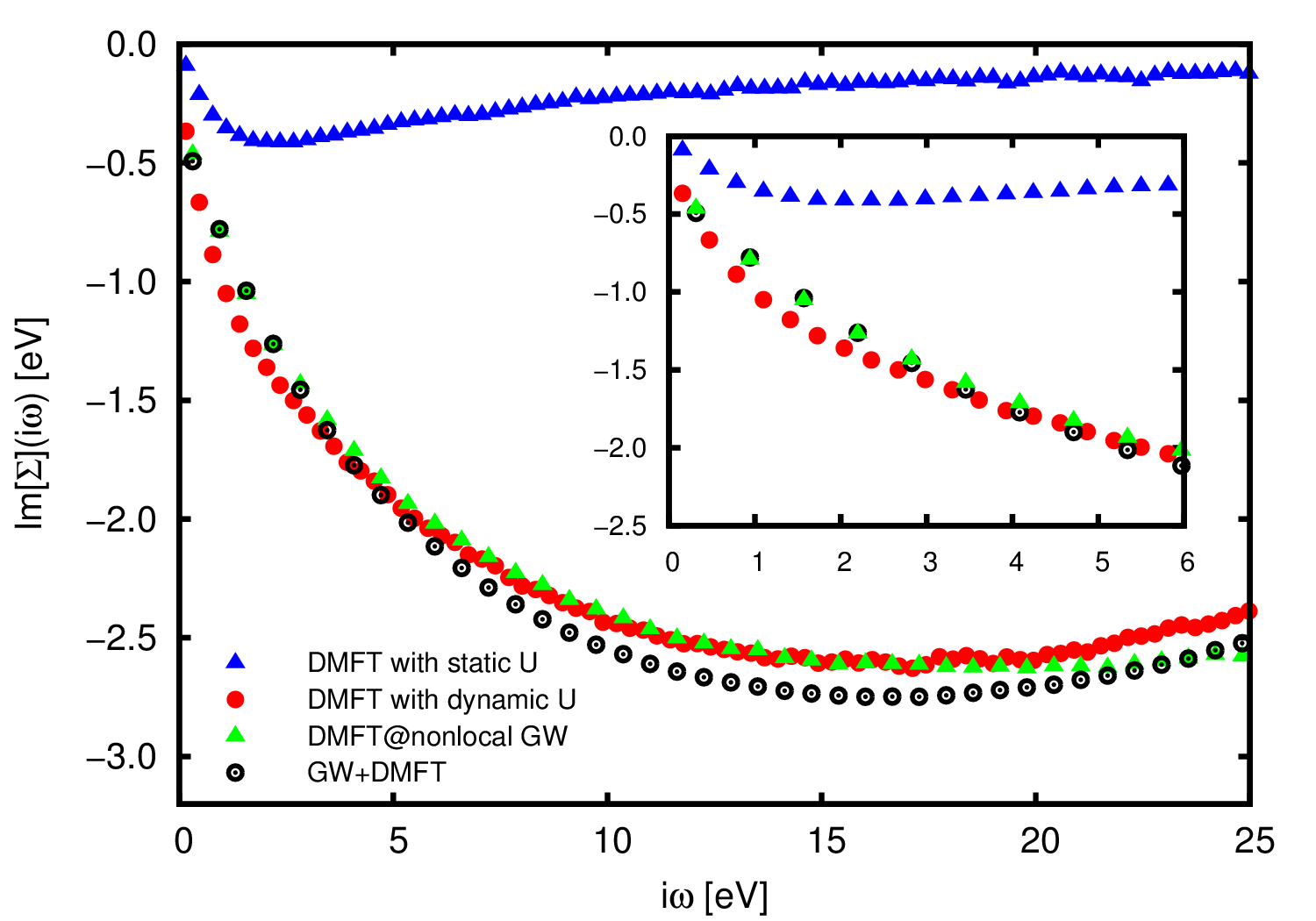
Figure 12: (Color online) Comparison of local t_2g self-energies on the Matsubara axis: usual LDA+DMFT, LDA+DMFT with dynamical interactions, DMFT@nonlocal GW and local part of full GW+DMFT.

Finally, we turn to a comparison of the contributions contained in the different schemes, on the basis of the local part of the Matsubara axis self-energies $\Sigma(i\omega)$, plotted in Fig. (12). The most striking feature in the comparison is the small amplitude of the standard LDA+DMFT self-energy. This can be trivially understood from the fact that only the partially screened value of the interaction, the Hubbard $U$, enters into the description. This scheme does not contain any information about the bare interaction – in contrast to all the other schemes, where it is recovered as the high-frequency limit. This information does lead to much higher characteristic energy scales in the schemes beyond LDA+DMFT, with self-energies living of the scale of the plasma energy of $\sim$ 15 eV.

When comparing the shape of the self-energies at low-energies, one can observe that the one for LDA+$\mathcal{U}(\omega)$+DMFT is slightly steeper, leading to an overestimation of the mass renormalization. The self-consistency loop in the full GW+DMFT scheme leads to a relaxation of the impurity self-energy, and thus less important renormalization effects. The change is in fact quite substantial, leading to different quasi-particle weights corresponding to the different self-energies: while the local $Z$ factor for the fully self-consistent GW+DMFT calculation is nearly 0.7, the LDA+DMFT calculation with dynamical $U$ yields 0.5. A non-selfconsistent calculation combining a local LDA+$\mathcal{U}(\omega)$+DMFT self-energy with a nonlocal-GW self-energy could therefore be expected to underestimate the bandwidth by a factor $0.7/0.5$. This may explain why a recent paper for SrVO₃Sakuma et al. (2013) using such a non-selfconsistent “[LDA+$\mathcal{U}(\omega)$+DMFT]_local+[GW]_nonlocal” approach finds a much narrower empty band than our GW+DMFT calculations. This puts strong constraints on the design of simplified schemes: it highlights the importance of having the nonlocal correlations present in the DMFT self-consistency, as done in the DMFT@nonlocal-GW discussed above, or also in the QSGW+DMFT schemeTomczak et al. (2012c).

Finally, DMFT@nonlocal-GW and full GW+DMFT are very close at low energies, as expected from the analysis above, but start to deviate on a scale of a few eV where the nonlocal self-energy correction on the real axis recovers some frequency-dependence. For obvious reasons, also a conceptually correct treatment of higher energy satellite features will require the use of the full GW+DMFT scheme.

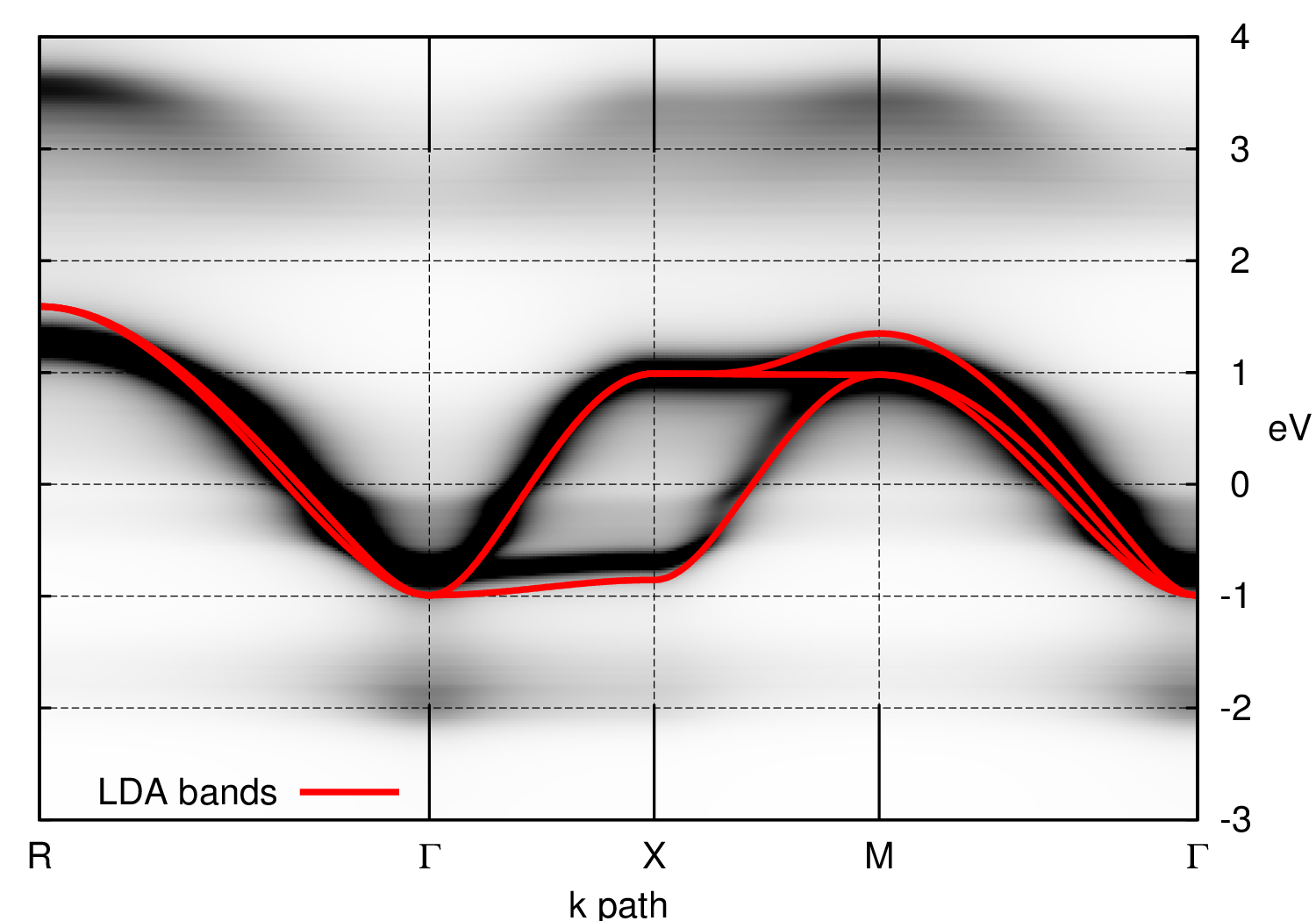
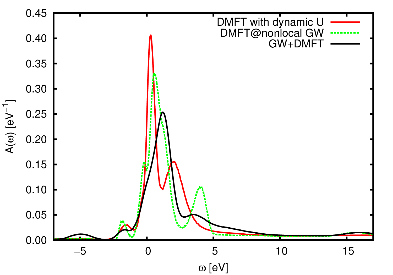
Figure 11: (Color online) Spectra using the DMFT@nonlocal-GW approach: resolved along a momentum path (left) and k-summed in comparison with the full GW+DMFT and LDA+$\mathcal{U}(\omega)$+DMFT.

V Summary

We now come back to the list of physics questions on our target compound, outlined in the introductory section on SrVO₃:

• Reconciliation of results of DMFT and cluster model calculations in the unoccupied part of the spectra, and consistency with ab initio $U$ values
  Our finding of the IPES peak at 2.7 eV being dominantly of e_g character, rather than being an upper Hubbard band of t_2g character, coincides with the interpretation of cluster model calculations Mossanek et al. (2009), thus reconciling DMFT with the cluster model literature. Cluster model calculations place an upper Hubbard band of t_2g character at about 2 eV, which would be consistent with the static value of $\mathcal{U}(\omega=0)=3.5$ eV. The cluster calculations, however, do not have access to the effects of the enhancement of the bare band dispersion by nonlocal exchange. Our GW+DMFT calculations reveal that the latter is in fact the dominant effect, preventing the formation of a clearly separated sharp upper Hubbard band.

• The 2.7eV feature in BIS spectra
   Related to the previous point, the photoemission feature at 2.7 eV is not an upper Hubbard band, but rather dominated by e_g states. It would be most interesting to perform orbital-resolved inverse photoemission studies to confirm this orbital assignment.

• Position of O2p ligand states
  The inclusion of the GW self-energy for the “uncorrelated” states, as explained in the section on the orbital-separated GW+DMFT scheme, introduces corrections on the O2p ligand states, which are pushed down in energy, improving the agreement with experiment. We note, however, that the size of the correction is not quite large enough, compared to experiment. To some extent, this could have been expected: indeed, we believe feedback effects of the Coulomb interactions on the V-d states (and their hybridization) to be important for determining the O2p position. However, such effects would only be included if an update of the GW part of the calculation were also performed. This observation thus opens important perspectives for further work.

• Position of Sr-4d states
  The Sr-d states are pushed up by the GW self-energy. The total O-p to Sr-d energetic distance is enhanced by about 1.25eV. Comparison with the experimental spectra shows that this correction is excellent in the unoccupied part of the spectrum.

Most importantly, however, we identify a substantial broadening of the unoccupied bandwidth with respect to standard LDA+DMFT calculations. Indeed, the nonlocal part of the GW self-energy, when applied as a correction to the LDA band structure, leads to a widening by more than 40 percent. When local correlations (within DMFT with $\mathcal{U}(\omega)$) are added, the corresponding renormalizations re-narrow the unoccupied band roughly such as to recover the original LDA bandwidth. For this reason, while being similar to the LDA+DMFT description for the occupied states, our results suggest an entirely new description for the unoccupied part of the spectrum, calling for a reinvestigation within techniques capturing empty states properties (BIS, IPES, time-resolved ARPES or similar).

VI Conclusions

We have implemented the combined GW+DMFT scheme in a fully dynamical manner, by treating the GW part at the one-shot level, but self-consisting over the DMFT part. Comparisons with pure LDA, pure GW, and LDA+DMFT calculations with static and dynamic interactions allow to assess the importance of the various features of these schemes, such as inclusion of dynamical screening, local and nonlocal self-energy contributions, and self-consistency.

In particular our analysis suggests that at low-energies, the dynamical self-energy contributions of GW or combined GW+DMFT schemes are strongly dominated by the local part, and that the crucial nonlocal corrections are a purely static correction to the LDA exchange correlation potential. This is strongly encouraging in view of the accuracy of DMFT-based schemes for correlated materials, and may allow for shortcuts when going beyond them (see e.g. the QSGW+DMFT schemeTomczak et al. (2012c)).

The calculated GW+DMFT spectral functions for SrVO₃ are in good agreement with available experimental data for the occupied electronic states. In this part of the spectra, the GW+DMFT scheme only leads to a slight improvement over conventional LDA+DMFT results (provided that in the latter the dynamics of the Hubbard $U$ is included).

Very importantly, however, our GW+DMFT results also suggest, that the unoccupied band structure is not well described by many-body calculations based on LDA-derived one-body Hamiltonians. Indeed, broadening by the Fock exchange term is substantial; the appropriate bare band structure for a DMFT-based electronic structure calculation should be wider by about 40 $\%$ than the corresponding LDA bands, so that the final dispersion after the many-body calculation is eventually comparable again to the LDA one.

The mechanism leading to these corrections is quite general: it is based on the simple observation that the exchange-correlation potential of DFT provides a much better approximation to (screened) exchange for occupied electronic states than for empty ones. This – quite generally – suggests that – despite their successes in describing occupied electronic states – many-body techniques based on LDA Hamiltonians are inappropriate for describing unoccupied states of correlated transition metal oxides. This is in particular true for the combined LDA+DMFT scheme.

These findings urgently call for experimental studies of correlated oxides by techniques suitable for measuring empty electronic states. Candidates could be bremsstrahl-isochromatography (BIS)/inverse photoemission, time-resolved ARPES, or more indirect probes such as resonant inelastic x-ray scattering (RIXS), optical spectroscopy, or x-ray absorption (XAS).

VII Acknowledgements

We acknowledge useful discussions with T. Ayral, A. Georges, M. Imada, A.I. Lichtenstein, C. Taranto, K. Held, as well as a collaboration with F. Aryasetiawan at the early stage of Ref. Tomczak et al., 2012b. This work was supported by the French ANR under projects SURMOTT and PNICTIDES and IDRIS/GENCI under projects 139313 and 096493. JMT acknowledges support from the European Research Council under the European Union’s Seventh Framework Programme (FP/2007-2013)/ERC through grant n. 306447.

VII.1 Appendix: The GW+DMFT Equations

As discussed in Sec. II.2, the GW+DMFT scheme as formulated in Refs. Biermann et al., 2003; Aryasetiawan et al., 2004b; Biermann et al., 2004b can be derived as a stationary point $(G,W)$ of the Almbladh free energy functional ALMBLADH et al. (1999) after approximating the correlation part of this functional by a combination of local and nonlocal terms stemming from DMFT and GW, respectively.

For reference, we here review the equations derived from this construction, leading to an iterative loop which determines ${\cal G}$ and ${\cal U}$ self-consistently (and, eventually, the full self-energy and polarization operators):

• The impurity problem (II.2) is solved, for a given choice of ${\cal G}_{LL^{\prime}}$ and ${\cal U}_{\alpha\beta}$: the “impurity” Green’s function

  $$G_{imp}^{LL^{\prime}}\equiv-\langle T_{\tau}c_{L}(\tau)c^{+}_{L^{\prime}}(\tau^{\prime})\rangle_{S}$$ (51)

  is calculated, together with the impurity self-energy

  $$\Sigma^{xc}_{imp}\equiv\delta\Psi_{imp}/\delta G_{imp}={\cal G}^{-1}-G_{imp}^{-1}.$$ (52)

  The two-particle correlation function

  $$\chi_{L_{1}L_{2}L_{3}L_{4}}=\langle:c^{\dagger}_{L_{1}}(\tau)c_{L_{2}}(\tau)::c^{\dagger}_{L_{3}}(\tau^{\prime})c_{L_{4}}(\tau^{\prime}):\rangle_{S}$$ (53)

  must also be evaluated.

• The impurity effective interaction is constructed as follows:

  $$W_{imp}^{\alpha\beta}={\cal U}_{\alpha\beta}-\sum_{L_{1}\cdots L_{4}}\sum_{\gamma\delta}{\cal U}_{\alpha\gamma}O^{\gamma}_{L_{1}L_{2}}\chi_{L_{1}L_{2}L_{3}L_{4}}[O^{\delta}_{L_{3}L_{4}}]^{*}{\cal U}_{\delta\beta}$$ (54)

  where $O_{L_{1}L_{2}}^{\alpha}\equiv\langle\phi_{L_{1}}\phi_{L_{2}}|B^{\alpha}\rangle$ is the overlap matrix between two-particle states and products of one-particle basis functions. The polarization operator of the impurity problem is then obtained as:

  $$P_{imp}\equiv-2\delta\Psi_{imp}/\delta W_{imp}={\cal U}^{-1}-W_{imp}^{-1},$$ (55)

  where all matrix inversions are performed in the two-particle basis $B^{\alpha}$ (see the discussion in Aryasetiawan et al. (2004b); Biermann et al. (2004b)).

• From Eqs. (II.2) and (II.2) the full ${\bf k}$-dependent Green’s function $G({\bf k},i\omega_{n})$ and effective interaction $W({\bf q},i\nu_{n})$ can be constructed. The self-consistency condition is obtained, as in the usual DMFT context, by requiring that the on-site components of these quantities coincide with $G_{imp}$ and $W_{imp}$. In practice, this is done by computing the on-site quantities

  $$G^{loc}(i\omega_{n}) = \sum_{\bf k}[{G_{H}}^{-1}({\bf k},i\omega_{n})-\Sigma^{xc}({\bf k},i\omega_{n})]^{-1}$$ (56)

  $$W^{loc}(i\nu_{n}) = \sum_{\bf q}[V_{{\bf q}}^{-1}-P({\bf q},i\nu_{n})]^{-1}$$ (57)

  and using them to update the Weiss dynamical mean field ${\cal G}$ and the impurity model interaction ${\cal U}$ according to:

  $${\cal G}^{-1}={G^{loc}}^{-1}+\Sigma^{xc}_{imp}$$ (58)

  $${\cal U}^{-1}={W^{loc}}^{-1}+P_{imp}$$ (59)

The set of equations (51) to (59) (including (12) and (13)) is iterated until self-consistency.

This in fact means that, conceptually, there are two levels of self-consistency: the one over local quantities, for a given GW calculation, and, eventually, also the update of non-local quantities by recalculation the GW self-energies and polarisation. In real materials calculations, this full self-consistency has been only performed once so far, namely in the relatively simple case of a single-orbital system Hansmann et al. (2013). Here, we restrict ourselves to self-consistency at the DMFT level for a given GW calculation, as discussed in the methodological sections above.

References

- Lichtenstein and Katsnelson (1998) A. I. Lichtenstein and M. I. Katsnelson, Phys. Rev. B 57, 6884 (1998).
- Anisimov et al. (1997) V. I. Anisimov, A. I. Poteryaev, M. A. Korotin, A. O. Anokhin, and G. Kotliar, J. Phys.: Cond. Matter 9, 7359 (1997).
- Biermann (2006) S. Biermann, in Encyclopedia of Materials: Science and Technology, edited by K. H. J. Buschow, R. W. Cahn, M. C. Flemings, B. I. (print), E. J. Kramer, S. Mahajan, , and P. V. (updates) (Elsevier, Oxford, 2006) pp. 1 – 9.
- Held et al. (2006) K. Held, I. A. Nekrasov, G. Keller, V. Eyert, N. Blümer, A. K. McMahan, R. T. Scalettar, T. Pruschke, V. I. Anisimov, and D. Vollhardt, physica status solidi (b) 243 (2006), psi-k Newsletter, 56 (65) 2003.
- ani (2000) (Editor: V. I. Anisimov. Amsterdam, The Netherlands : Gordon and Breach Science Publishers, 2000).
- Kotliar and Vollhardt (2004) G. Kotliar and D. Vollhardt, Physics Today 57, 53 (2004).
- Lichtenstein et al. (2001) A. I. Lichtenstein, M. I. Katsnelson, and G. Kotliar, Phys. Rev. Lett. 87, 067205 (2001).
- Biermann et al. (2004a) S. Biermann, A. Dallmeyer, C. Carbone, W. Eberhardt, C. Pampuch, O. Rader, M. I. Katsnelson, and A. I. Lichtenstein, JETP Letters 80, 612 (2004a), condmat0112430.
- Liebsch (2003) A. Liebsch, Phys. Rev. Lett. 90, 096401 (2003).
- Pavarini et al. (2004) E. Pavarini, S. Biermann, A. Poteryaev, A. I. Lichtenstein, A. Georges, and O. K. Andersen, Phys. Rev. Lett. 92, 176403 (2004).
- Held et al. (2001a) K. Held, G. Keller, V. Eyert, D. Vollhardt, and V. I. Anisimov, Phys. Rev. Lett. 86, 5345 (2001a).
- Keller et al. (2004) G. Keller, K. Held, V. Eyert, D. Vollhardt, and V. I. Anisimov, Phys. Rev. B 70, 205116 (2004).
- Poteryaev et al. (2007) A. I. Poteryaev, J. M. Tomczak, S. Biermann, A. Georges, A. I. Lichtenstein, A. N. Rubtsov, T. Saha-Dasgupta, and O. K. Andersen, Phys. Rev. B 76, 085127 (2007), preprint arXiv:cond-mat/0701263.
- Nekrasov et al. (2005) I. A. Nekrasov, G. Keller, D. E. Kondakov, A. V. Kozhevnikov, T. Pruschke, K. Held, D. Vollhardt, and V. I. Anisimov, Phys. Rev. B 72, 155106 (2005).
- Tomczak and Biermann (2009a) J. M. Tomczak and S. Biermann, J. Phys.: Cond. Matter 21 (2009a), preprint arXiv:0811.1098.
- Nekrasov et al. (2006) I. A. Nekrasov, K. Held, G. Keller, D. E. Kondakov, T. Pruschke, M. Kollar, O. K. Andersen, V. I. Anisimov, and D. Vollhardt, Phys. Rev. B 73, 155112 (2006).
- Saha-Dasgupta et al. (2005) T. Saha-Dasgupta, A. Lichtenstein, and R. Valentí, Phys. Rev. B 71, 153108 (2005).
- Rodolakis et al. (2010) F. Rodolakis, P. Hansmann, J.-P. Rueff, A. Toschi, M. W. Haverkort, G. Sangiovanni, A. Tanaka, T. Saha-Dasgupta, O. K. Andersen, K. Held, M. Sikora, I. Alliot, J.-P. Itié, F. Baudelet, P. Wzietek, P. Metcalf, and M. Marsi, Phys. Rev. Lett. 104, 047401 (2010).
- Hansmann et al. (2012) P. Hansmann, M. W. Haverkort, A. Toschi, G. Sangiovanni, F. Rodolakis, J. P. Rueff, M. Marsi, and K. Held, Phys. Rev. B 85, 115136 (2012).
- Wang et al. (2012) X. Wang, M. J. Han, L. de’ Medici, H. Park, C. A. Marianetti, and A. J. Millis, Phys. Rev. B 86, 195136 (2012).
- Zhang et al. (2012) G. Zhang, E. Gorelov, E. Koch, and E. Pavarini, Phys. Rev. B 86, 184413 (2012).
- Flesch et al. (2012) A. Flesch, G. Zhang, E. Koch, and E. Pavarini, Phys. Rev. B 85, 035124 (2012).
- Gorelov et al. (2010) E. Gorelov, M. Karolak, T. O. Wehling, F. Lechermann, A. I. Lichtenstein, and E. Pavarini, Phys. Rev. Lett. 104, 226401 (2010).
- Pavarini and Koch (2010) E. Pavarini and E. Koch, Phys. Rev. Lett. 104, 086402 (2010).
- De Raychaudhury et al. (2007) M. De Raychaudhury, E. Pavarini, and O. K. Andersen, Phys. Rev. Lett. 99, 126402 (2007).
- Kuneš et al. (2009) J. Kuneš, D. M. Korotin, M. A. Korotin, V. I. Anisimov, and P. Werner, Phys. Rev. Lett. 102, 146402 (2009).
- Augustinský et al. (2013) P. Augustinský, V. Křápek, and J. Kuneš, Phys. Rev. Lett. 110, 267204 (2013).
- Biermann et al. (2005) S. Biermann, A. Poteryaev, A. I. Lichtenstein, and A. Georges, Phys. Rev. Lett. 94, 026404 (2005).
- Tomczak and Biermann (2009b) J. M. Tomczak and S. Biermann, Phys. Status Solidi B (feature article) 246, 1996 (2009b), scientific Highlight of the Month of the Network, no. 88, August 2008, arXiv:0907.1575.
- Tomczak and Biermann (2009c) J. M. Tomczak and S. Biermann, Europhys. Lett. 86, 37004 (2009c), preprint arXiv:0807.4044.
- Lechermann et al. (2005) F. Lechermann, S. Biermann, and A. Georges, Phys. Rev. Lett. 94, 166402 (2005).
- Lechermann et al. (2007) F. Lechermann, S. Biermann, and A. Georges, Phys. Rev. B 76, 085101 (2007).
- Tomczak et al. (2012a) J. M. Tomczak, K. Haule, and G. Kotliar, Proc. Natl. Acad. Sci. USA 109, 3243 (2012a), preprint arXiv:1109.6561, http://www.pnas.org/content/109/9/3243.full.pdf+html .
- Tomczak et al. (2013a) J. M. Tomczak, K. Haule, and G. Kotliar, in New Materials for Thermoelectric Applications: Theory and Experiment, NATO Science for Peace and Security Series B: Physics and Biophysics, edited by V. Zlatić and A. Hewson (Springer Netherlands, 2013) pp. 45–57, preprint arXiv:1210.3379.
- Miyake et al. (2008) T. Miyake, L. Pourovskii, V. Vildosola, S. Biermann, and A. Georges, J. Phys. Soc. Jpn. 77SC, 99 (2008).
- Tomczak et al. (2013b) J. M. Tomczak, L. V. Pourovskii, L. Vaugier, A. Georges, and S. Biermann, Proc. Natl. Acad. Sci. USA 110, 904 (2013b), preprint arXiv:1301.0630, http://www.pnas.org/content/110/3/904.full.pdf+html .
- Savrasov et al. (2001) S. Y. Savrasov, G. Kotliar, and E. Abrahams, Nature 410, 793 (2001).
- Held et al. (2001b) K. Held, A. K. McMahan, and R. T. Scalettar, Phys. Rev. Lett. 87, 276404 (2001b).
- Haule et al. (2008) K. Haule, J. H. Shim, and G. Kotliar, Phys. Rev. Lett. 100, 226402 (2008).
- Skornyakov et al. (2009) S. L. Skornyakov, A. V. Efremov, N. A. Skorikov, M. A. Korotin, Y. A. Izyumov, V. I. Anisimov, A. V. Kozhevnikov, and D. Vollhardt, Phys. Rev. B 80, 092501 (2009).
- Anisimov et al. (2009) V. I. Anisimov, D. M. Korotin, M. A. Korotin, A. V. Kozhevnikov, J. Kunes, A. O. Shorikov, S. L. Skornyakov, and S. V. Streltsov, Journal of Physics: Condensed Matter 21, 075602 (7pp) (2009).
- Aichhorn et al. (2009) M. Aichhorn, L. Pourovskii, V. Vildosola, M. Ferrero, O. Parcollet, T. Miyake, A. Georges, and S. Biermann, Phys. Rev. B 80, 085101 (2009).
- Aichhorn et al. (2010) M. Aichhorn, S. Biermann, T. Miyake, A. Georges, and M. Imada, Phys. Rev. B 82, 064504 (2010).
- Hansmann et al. (2010) P. Hansmann, R. Arita, A. Toschi, S. Sakai, G. Sangiovanni, and K. Held, Phys. Rev. Lett. 104, 197002 (2010).
- Lee et al. (2010) H. Lee, Y.-Z. Zhang, H. O. Jeschke, and R. Valentí, Phys. Rev. B 81, 220506 (2010).
- Ferber et al. (2012) J. Ferber, K. Foyevtsova, R. Valentí, and H. O. Jeschke, Phys. Rev. B 85, 094505 (2012).
- Werner et al. (2012) P. Werner, M. Casula, T. Miyake, F. Aryasetiawan, A. J. Millis, and S. Biermann, Nat. Phys. 8, 331 (2012).
- Martins et al. (2011) C. Martins, M. Aichhorn, L. Vaugier, and S. Biermann, Phys. Rev. Lett. 107, 266404 (2011).
- Ayral et al. (2012) T. Ayral, P. Werner, and S. Biermann, Phys. Rev. Lett. 109, 226401 (2012).
- Ayral et al. (2013) T. Ayral, S. Biermann, and P. Werner, Phys. Rev. B 87, 125149 (2013).
- Hansmann et al. (2013) P. Hansmann, T. Ayral, L. Vaugier, P. Werner, and S. Biermann, Phys. Rev. Lett. 110, 166401 (2013).
- Casula et al. (2012a) M. Casula, P. Werner, L. Vaugier, F. Aryasetiawan, T. Miyake, A. J. Millis, and S. Biermann, Phys. Rev. Lett. 109, 126408 (2012a).
- Aryasetiawan et al. (2004a) F. Aryasetiawan, M. Imada, A. Georges, G. Kotliar, S. Biermann, and A. I. Lichtenstein, Phys. Rev. B 70, 195104 (2004a).
- Casula et al. (2012b) M. Casula, A. Rubtsov, and S. Biermann, Phys. Rev. B 85, 035115 (2012b).
- Biermann et al. (2003) S. Biermann, F. Aryasetiawan, and A. Georges, Phys. Rev. Lett. 90, 086402 (2003).
- Tomczak et al. (2012b) J. M. Tomczak, M. Casula, T. Miyake, F. Aryasetiawan, and S. Biermann, EPL (Europhysics Letters) 100, 67001 (2012b), “EPL editor’s choice”, preprint arXiv:1210.6580.
- Karlsson (2005) K. Karlsson, Journal of Physics: Condensed Matter 17, 7573 (2005).
- Taranto et al. (2013) C. Taranto, M. Kaltak, N. Parragh, G. Sangiovanni, G. Kresse, A. Toschi, and K. Held, Phys. Rev. B 88, 165119 (2013).
- Werner and Millis (2010) P. Werner and A. J. Millis, Phys. Rev. Lett. 104, 146401 (2010).
- Hedin (1965) L. Hedin, Phys. Rev. 139, A796 (1965).
- Note (1) The notion of locality refers to the use of a specific basis set of atom-centered orbitals, such as muffin-tin orbitals, or atom-centered Wannier functions.
- Note (2) See also the related scheme of Ref. \rev@citealpnumPhysRevB.66.085120 and the comparison to GW+DMFT in Ref. \rev@citealpnumPhysRevB.87.125149.
- Biermann et al. (2004b) S. Biermann, F. Aryasetiawan, and A. Georges, Proceedings of the NATO Advanced Research Workshop on ”Physics of Spin in Solids: Materials, Methods, and Applications” in Baku, Azerbaijan, Oct. 2003. NATO Science Series II, Kluwer Academic Publishers B.V (2004b).
- Aryasetiawan et al. (2004b) F. Aryasetiawan, S. Biermann, and A. Georges, Proceedings of the conference ”Coincidence Studies of Surfaces, Thin Films and Nanostructures”, Ringberg castle, Sept. 2003 (2004b).
- ALMBLADH et al. (1999) C.-O. ALMBLADH, U. V. BARTH, and R. V. LEEUWEN, Int. J. Mod. Phys. B 13, 535 (1999).
- Chitra and Kotliar (2001) R. Chitra and G. Kotliar, Phys. Rev. B 63, 115110 (2001).
- Hendrik (1996) K. Hendrik, (PhD thesis, Rutgers University, 1996).
- Si and Smith (1996) Q. Si and J. L. Smith, Phys. Rev. Lett. 77, 3391 (1996).
- Sengupta and Georges (1995) A. M. Sengupta and A. Georges, Phys. Rev. B 52, 10295 (1995).
- Aryasetiawan et al. (2009) F. Aryasetiawan, J. M. Tomczak, T. Miyake, and R. Sakuma, Phys. Rev. Lett. 102, 176402 (2009), preprint arXiv:0806.3373.
- Souza et al. (2001) I. Souza, N. Marzari, and D. Vanderbilt, Phys. Rev. B 65, 035109 (2001).
- Marzari et al. (2012) N. Marzari, A. A. Mostofi, J. R. Yates, I. Souza, and D. Vanderbilt, Rev. Mod. Phys. 84, 1419 (2012).
- Imada et al. (1998) M. Imada, A. Fujimori, and Y. Tokura, Rev. Mod. Phys. 70, 1039 (1998).
- Onoda et al. (1991) M. Onoda, H. Ohta, and H. Nagasawa, Solid State Communications 79, 281 (1991).
- Inoue et al. (1997) I. Inoue, H. Makino, I. Hase, M. Ishikawa, N. Hussey, and M. Rozenberg, Physica B: Condensed Matter 237–238, 61 (1997), ¡ce:title¿Proceedings of the Yamada Conference XLV, the International Conference on the Physics of Transition Metals¡/ce:title¿.
- Eisaki (1991) H. Eisaki, (PhD thesis, Tokyo University, 1991).
- Sekiyama et al. (2004) A. Sekiyama, H. Fujiwara, S. Imada, S. Suga, H. Eisaki, S. I. Uchida, K. Takegahara, H. Harima, Y. Saitoh, I. A. Nekrasov, G. Keller, D. E. Kondakov, A. V. Kozhevnikov, T. Pruschke, K. Held, D. Vollhardt, and V. I. Anisimov, Phys. Rev. Lett. 93, 156402 (2004).
- Morikawa et al. (1995) K. Morikawa, T. Mizokawa, K. Kobayashi, A. Fujimori, H. Eisaki, S. Uchida, F. Iga, and Y. Nishihara, Phys. Rev. B 52, 13711 (1995).
- Fujimori et al. (1992) A. Fujimori, I. Hase, H. Namatame, Y. Fujishima, Y. Tokura, H. Eisaki, S. Uchida, K. Takegahara, and F. M. F. de Groot, Phys. Rev. Lett. 69, 1796 (1992).
- Georges et al. (1996) A. Georges, G. Kotliar, W. Krauth, and M. J. Rozenberg, Rev. Mod. Phys. 68, 13 (1996).
- Müller-Hartmann (1989) E. Müller-Hartmann, Zeitschrift für Physik B Condensed Matter 76, 211 (1989).
- Inoue (1998) I. Inoue, Electronic States of Correlated Transition Metal Oxides: Ca1-xSrxVO3 and Sr2RuO4 (PhD thesis, Tokyo University, 1998).
- Inoue et al. (1998) I. H. Inoue, O. Goto, H. Makino, N. E. Hussey, and M. Ishikawa, Phys. Rev. B 58, 4372 (1998).
- Maiti et al. (2001) K. Maiti, D. D. Sarma, M. J. Rozenberg, I. H. Inoue, H. Makino, O. Goto, M. Pedio, and R. Cimino, EPL (Europhysics Letters) 55, 246 (2001).
- Maiti et al. (2006) K. Maiti, U. Manju, S. Ray, P. Mahadevan, I. H. Inoue, C. Carbone, and D. D. Sarma, Phys. Rev. B 73, 052508 (2006).
- Pavarini et al. (2005) E. Pavarini, A. Yamasaki, J. Nuss, and O. K. Andersen, New Journal of Physics 7, 188 (2005).
- Ishida et al. (2006) H. Ishida, D. Wortmann, and A. Liebsch, Phys. Rev. B 73, 245421 (2006).
- Yoshida et al. (2005) T. Yoshida, K. Tanaka, H. Yagi, A. Ino, H. Eisaki, A. Fujimori, and Z.-X. Shen, Phys. Rev. Lett. 95, 146404 (2005).
- Eguchi et al. (2006) R. Eguchi, T. Kiss, S. Tsuda, T. Shimojima, T. Mizokami, T. Yokoya, A. Chainani, S. Shin, I. H. Inoue, T. Togashi, S. Watanabe, C. Q. Zhang, C. T. Chen, M. Arita, K. Shimada, H. Namatame, and M. Taniguchi, Phys. Rev. Lett. 96, 076402 (2006).
- Zhang and Imada (2007) Y. Z. Zhang and M. Imada, Phys. Rev. B 76, 045108 (2007).
- Lee et al. (2012) H. Lee, K. Foyevtsova, J. Ferber, M. Aichhorn, H. O. Jeschke, and R. Valentí, Phys. Rev. B 85, 165103 (2012).
- Takizawa et al. (2009) M. Takizawa, M. Minohara, H. Kumigashira, D. Toyota, M. Oshima, H. Wadati, T. Yoshida, A. Fujimori, M. Lippmaa, M. Kawasaki, H. Koinuma, G. Sordi, and M. Rozenberg, Phys. Rev. B 80, 235104 (2009).
- Yoshida et al. (2010) T. Yoshida, M. Hashimoto, T. Takizawa, A. Fujimori, M. Kubota, K. Ono, and H. Eisaki, Phys. Rev. B 82, 085119 (2010).
- Yoshimatsu et al. (2010) K. Yoshimatsu, T. Okabe, H. Kumigashira, S. Okamoto, S. Aizaki, A. Fujimori, and M. Oshima, Phys. Rev. Lett. 104, 147601 (2010).
- Zhong et al. (2013) Z. Zhong, M. Wallerberger, J. M. Tomczak, C. Taranto, N. Parragh, A. Toschi, G. Sangiovanni, and K. Held, ArXiv e-prints (2013), arXiv:1312.5989 [cond-mat.str-el] .
- Aizaki et al. (2012) S. Aizaki, T. Yoshida, K. Yoshimatsu, M. Takizawa, M. Minohara, S. Ideta, A. Fujimori, K. Gupta, P. Mahadevan, K. Horiba, H. Kumigashira, and M. Oshima, Phys. Rev. Lett. 109, 056401 (2012).
- Lechermann et al. (2006) F. Lechermann, A. Georges, A. Poteryaev, S. Biermann, M. Posternak, A. Yamasaki, and O. K. Andersen, Phys. Rev. B 74, 125120 (2006).
- Trimarchi et al. (2008) G. Trimarchi, I. Leonov, N. Binggeli, D. Korotin, and V. I. Anisimov, Journal of Physics: Condensed Matter 20, 135227 (2008).
- Amadon et al. (2008) B. Amadon, F. Lechermann, A. Georges, F. Jollet, T. O. Wehling, and A. I. Lichtenstein, Phys. Rev. B 77, 205112 (2008).
- Karolak et al. (2011) M. Karolak, T. O. Wehling, F. Lechermann, and A. I. Lichtenstein, Journal of Physics: Condensed Matter 23, 085601 (2011).
- Byczuk et al. (2007) K. Byczuk, M. Kollar, K. Held, Y. F. Yang, I. A. Nekrasov, T. Pruschke, and D. Vollhardt, Nat Phys 3, 168 (2007).
- Eguchi et al. (2009) R. Eguchi, A. Chainani, M. Taguchi, M. Matsunami, Y. Ishida, K. Horiba, Y. Senba, H. Ohashi, and S. Shin, Phys. Rev. B 79, 115122 (2009).
- Deng et al. (2012) X. Deng, M. Ferrero, J. Mravlje, M. Aichhorn, and A. Georges, Phys. Rev. B 85, 125137 (2012).
- Deng et al. (2009) X. Deng, L. Wang, X. Dai, and Z. Fang, Phys. Rev. B 79, 075114 (2009).
- Mossanek et al. (2006) R. J. O. Mossanek, M. Abbate, and A. Fujimori, Phys. Rev. B 74, 155127 (2006).
- Mossanek et al. (2009) R. J. O. Mossanek, M. Abbate, T. Yoshida, A. Fujimori, Y. Yoshida, N. Shirakawa, H. Eisaki, S. Kohno, P. T. Fonseca, and F. C. Vicentin, Phys. Rev. B 79, 033104 (2009).
- Mossanek et al. (2008) R. J. O. Mossanek, M. Abbate, T. Yoshida, A. Fujimori, Y. Yoshida, N. Shirakawa, H. Eisaki, S. Kohno, and F. C. Vicentin, Phys. Rev. B 78, 075103 (2008).
- Wadati et al. (2009) H. Wadati, A. Chikamatsu, M. Takizawa, H. Kumigashira, T. Yoshida, T. Mizokawa, A. Fujimori, M. Oshima, and N. Hamada, J. Phys. Soc. Jpn. 78, 094709 (2009).
- Aryasetiawan et al. (2006) F. Aryasetiawan, K. Karlsson, O. Jepsen, and U. Schönberger, Phys. Rev. B 74, 125106 (2006).
- Miyake and Aryasetiawan (2008a) T. Miyake and F. Aryasetiawan, Phys. Rev. B 77, 085122 (2008a).
- Huang and Wang (2012) L. Huang and Y. Wang, EPL (Europhysics Letters) 99, 67003 (2012).
- van Benthem et al. (2001) K. van Benthem, C. Elsässer, and R. H. French, Journal of Applied Physics 90, 6156 (2001).
- Gatti and Guzzo (2013) M. Gatti and M. Guzzo, Phys. Rev. B 87, 155147 (2013).
- Note (3) See e.g. Taranto et al. Taranto et al. (2013) for a study exploring the limits of an implementation with static Hubbard interactions, and – most recently – Sakuma et al. Sakuma et al. (2013) who investigated the ad hoc combination of an LDA++DMFT self-energy with a GW one.
- Kohiki et al. (2000) S. Kohiki, M. Arai, H. Yoshikawa, S. Fukushima, M. Oku, and Y. Waseda, Phys. Rev. B 62, 7964 (2000).
- Nomura et al. (2012) Y. Nomura, M. Kaltak, K. Nakamura, C. Taranto, S. Sakai, A. Toschi, R. Arita, K. Held, G. Kresse, and M. Imada, Phys. Rev. B 86, 085117 (2012).
- Tomczak et al. (2012c) J. M. Tomczak, M. van Schilfgaarde, and G. Kotliar, Phys. Rev. Lett. 109, 237010 (2012c), preprint arXiv:1209.2213.
- Note (4) Of course, the LDA+DMFT self-energy will acquire a trivial momentum dependence when transformed from the local into the Kohn-Sham basis, which is owing to the change in orbital characters for varying momenta.
- Note (5) It can be shown that the linear increase of away from the Fermi level stems from the momentum dependence of -corrections to .
- Note (6) Nonlocal correlation effects beyond the GW picture, stemming e.g. from fluctuations in the spin-channel, are not included in this discussion. Also, the energy range of validity of the Fermi liquid regime is generally overestimated within the GW approximation, confining the argument to lower energies than suggested by the GW picture.
- Faleev et al. (2004) S. V. Faleev, M. van Schilfgaarde, and T. Kotani, Phys. Rev. Lett. 93, 126406 (2004).
- Note (7) Naturally, a nonlocal dynamics is expected in lower dimensional systems, when spin fluctuations (not accounted for in GW) become important, e.g. in the quasi-2d cuprates. In Refs. \rev@citealpnumayral_gwdmft,PhysRevB.87.125149,PhysRevB.87.125149, for example, it was found that nonlocal self-energy effects obtained from fluctuations in the charge channel are small within GW+DMFT calculations of an extended Hubbard model, indicating that the leading nonlocal corrections are in the spin- rather than the charge-channel.
- Zein et al. (2006) N. E. Zein, S. Y. Savrasov, and G. Kotliar, Phys. Rev. Lett. 96, 226403 (2006).
- Note (8) See, however, the preceding footnote.
- Miyake and Aryasetiawan (2008b) T. Miyake and F. Aryasetiawan, Phys. Rev. B 77, 085122 (2008b).
- Sakuma et al. (2013) R. Sakuma, P. Werner, and F. Aryasetiawan, Phys. Rev. B 88, 235110 (2013).
- Sun and Kotliar (2002) P. Sun and G. Kotliar, Phys. Rev. B 66, 085120 (2002).