Sudakov Factor in the Deep Inelastic Scattering
of a Current off a Large Nucleus

Abstract

We consider a gedanken experiment of the scattering of a current $j=-\frac{1}{4}F^{i}_{\mu\nu}F^{i}_{\mu\nu}$ off a large nucleus to study the gluon saturation at the small-$x$ limit and compute the Sudakov factor of this process through a one-loop calculation. The differential cross section is expressed in term of the Sudakov resummation, in which the collinear and the rapidity divergences are subtracted. We also discuss how to probe the Weizsäcker-Williams (WW) gluon distribution in the process of photon pair production in the $pA$ collisions.

I Introduction

Saturation physicsGribov:1984tu ; Mueller:1989st has been one of the most interesting topics in high energy nuclear physics corresponding the small-$x$ physics. It describes the rapid rise of parton distributions at very high energy Balitsky:1978ic ; Kuraev:1977fs . In addition, by including the non-linear evolutionMueller:1985wy ; Balitsky:1995ub ; JalilianMarian:1997jx dynamics when the gluon distribution becomes order $1/\alpha_{s}$, parton distributions start to saturate as the scattering amplitude approaches unitarity. There are many phenomenological models to describe the dynamics inside the nucleuses in small-$x$ physics, the semi-classic model named color glass condensate (CGC) has been widely used to describe the dynamics inside the nucleus in the small-$x$ physicsIancu:2000hn .
The Sudakov resummation has been widely used in various high energy physics processesSudakov:1954sw ; Collins:1984kg ; Davies:1984sp , in the meantime, the small-$x$ logarithms $\alpha_{s}\ln{1/x_{g}}$ are also important, and normally resummed through small-$x$ evolution equations. It has been demonstrated that Sudakov type large logarithms and small-$x$ type logarithms can be resummed independently in various physics processes, for example, the Higgs production and dijet in $pA$ collisionsMueller:2012uf ; Mueller:2013uf .
The so-called Weizäcker-Williams (WW) gluon distributionCollins:1981uw ; McLerran:1993ni ; Ji:2005nu ; Dominguez:2011gc , which is the genuine gluon distribution, only appears in the observables if the initial or the final state interaction is absent in the inelastic scattering of the gluonic current on a nucleus target. For example, in the photon pair production in $pA$ collisions, where the final interaction is absent, the WW gluon distribution appears.
The objective of this calculation is to investigate the DIS of the gluonic current off a large nucleus and the photon pair production in $pA$ collisions. The common feature of these two processes is that they are both involving the so-called WW gluon distribution at small-$x$ limit. This paper can be considered as a supplementary study of the Ref. Mueller:2013uf .
The paper is organized into five sections, we start with introduction, The section II is about the leading order of DIS of gluonic current off a large nucleus. The details of calculation of the Sudakov factor will be presented in section III, we discuss how to probe the WW gluon distribution in the process of photon pair production in $pA$ collisions in section IV, in section V, we conclude with discussions on Sudakov resummmation and WW gluon distribution.

II Leading order in DIS of Current off a large nucleus

First, we consider a gedanken experiment of deep inelastic scattering (DIS) of the gluonic current of $j(x)=-\frac{1}{4}F^{i}_{\mu\nu}(x)F^{i}_{\mu\nu}(x)$ off a large nucleus at the leading orderMueller:1989st ; Kovchegov:1998bi , where $F^{i}_{\mu\nu}(x)$ is the QCD field strength tensor. This current is chosen because it is easy to study the WW gluon distribution in this process. The feynman diagram of DIS of the gluonic current off a large nucleus is in Fig. 1, the momentum of the gluonic current is $q$, we can treat the current as a scalar particle, the momentum square of the current satisfies $q^{2}=-Q^{2}$, and the virtual mass of the current is $M=iQ$, the notation of $q$ in the light cone gauge is

$$q^{\mu}=\left(q^{+},\frac{-Q^{2}}{2q^{+}},0\right).$$ (1)

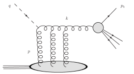
Figure 1: Feynman diagram at leading order of deep inelastic scattering of the current off a large nucleus.

We define $k$ as momentum of the final state produced gluon(the horizontal gluon in Fig. 1), $P$ as momentum of the large nucleus, $p$ as momentum of the outgoing gluons(vertical gluons in Fig. 1) from the target nucleus. In this calculation, we assume that the plus component of $q$ and minus component of $P$ both are large. We define $p_{h}$ as momentum of the final state hadron, $y$ as the rapidity of final state hadron, and $z_{1}=p_{h}^{+}/k^{+}$. We can calculate the differential cross section by transverse momentum dependent(TMD) factorizationJi:2005nu ; Dominguez:2011wm , it reads

$$\frac{\text{d}\sigma^{jA\rightarrow h+X}_{\textrm{LO}}}{\sigma_{0}\text{d}y\text{d}^{2}p_{h\perp}} = \frac{D_{h/g}(z_{1})}{z^{2}_{1}}\int\frac{d^{2}x_{\perp}d^{2}x^{\prime}_{\perp}}{(2\pi)^{2}}\,e^{-ik_{\perp}\cdot(x_{\perp}-x^{\prime}_{\perp})}$$ (2)

$$\times S^{WW}(x_{\perp},x^{\prime}_{\perp}),$$

where $S^{ww}(x_{\perp},x^{\prime}_{\perp})$ is the WW gluon distribution in the coordinate space, it is defined as

$$S {}^{WW}(x_{\perp},x^{\prime}_{\perp})$$ (3)

$$=-\langle\text{Tr}[\partial^{i}U(x_{\perp})]U^{\dagger}(x^{\prime}_{\perp})[\partial^{i}U(x^{\prime}_{\perp})]U^{\dagger}(x_{\perp})\rangle_{x_{g}},$$

the fundamental Wilson line is defined as

$$U(x_{\perp})=\mathcal{P}\exp\left\{ig_{S}\int_{-\infty}^{+\infty}\text{d}x^{+}\,T^{c}A_{c}^{-}(x^{+},x_{\perp})\right\}\ ,$$ (4)

where $A_{c}^{-}(x^{+},x_{\perp})$ is gluon field solution of Yang-Mill equation. There is a $\delta(z_{1}-p_{h}^{+}/k^{+})$, which has been integrated by $z_{1}$. The $\sigma_{0}$ is the leading-order of the gluon production, and it reads $\sigma_{0}\propto 1/4g^{2}\left(1-\epsilon\right)$, where $\epsilon=(4-D)/2$. The kinematics of DIS of the gluonic current off a large nucleus target at leading-order satisfies

$$x_{g}s=Q^{2},$$ (5)

where $s=2P\cdot q$, and $x_{g}$ is longitudinal momentum fraction of the outgoing gluons to the nucleus target, we assume that $Q^{2}\gg k_{\perp}^{2}$, but keep $x_{g}\ll 1$. In addition, throughout this paper, we use leading power approximation, therefore, we neglect higher order power correction of order $k^{2}_{\perp}/Q^{2}$.

III Sudakov factor in DIS of current off a large nucleus

Now, we consider one-loop order of the process of DIS of current off a large nucleus, with the help of formalism of dipole modelMueller:1999wm , it is more convenient to do the calculation in coordinate space. In order to calculate the amplitude in coordinate space, some types of splitting functions are introduced at first, such as $\Psi_{g\to gg}\left(\xi,u_{\perp}\right)$ , $\Psi_{g\to q\bar{q}}\left(\xi,u_{\perp}\right)$ and $\Psi_{j\to gg}\left(\xi,u_{\perp}\right)$Mueller:2013uf ; Dominguez:2011wm .
The $j\rightarrow gg$ splitting function in momentum space and coordinate space are

$$\Psi_{j\rightarrow gg}\left(\xi,k_{\perp}\right) = \sqrt{\frac{1}{2\xi(1-\xi)k^{+}}}\frac{1}{k_{\perp}^{2}+\xi(1-\xi)Q^{2}}$$

$$\times\left(\frac{1}{2}k_{\perp}^{2}\epsilon_{\perp}^{(1)}\cdot\epsilon_{\perp}^{(2)}-k_{\perp}\cdot\epsilon_{\perp}^{(1)}k_{\perp}\cdot\epsilon_{\perp}^{(2)}\right),$$

and

$$\Psi_{j\rightarrow gg}\left(\xi,u_{\perp}\right) = -\sqrt{\frac{1}{2\xi(1-\xi)k^{+}}}\frac{2\pi}{u_{\perp}^{2}}K(\epsilon_{f}u_{\perp})$$

$$\times\left(\frac{1}{2}\epsilon_{\perp}^{(1)}\cdot\epsilon_{\perp}^{(2)}-\frac{1}{u_{\perp}^{2}}u_{\perp}\cdot\epsilon_{\perp}^{(1)}u_{\perp}\cdot\epsilon_{\perp}^{(2)}\right),$$

respectively, here $\xi$ and $1-\xi$ are fractions of the longitudinal momentum of the radiating gluons, $\epsilon_{\perp}^{(1)}$ and $\epsilon_{\perp}^{(2)}$ are polarizations of the radiating gluons, and $K(\epsilon_{f}u_{\perp})$ is defined as

$$K(\epsilon_{f}u_{\perp})=2\epsilon_{f}u_{\perp}\text{K}_{1}(\epsilon_{f}u_{\perp})+\epsilon_{f}^{2}u_{\perp}^{2}\text{K}_{0}(\epsilon_{f}u_{\perp}),$$ (8)

where $\epsilon_{f}^{2}=\xi(1-\xi)Q^{2}$ and $K_{0,1}$ are modified Bessel functions.
Because the scattering energy in the collisions is very high, the interaction time of multiply scattering is so short that the radiating gluon is either before or after the multiply scattering.

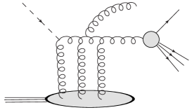
Figure 2: Radiating gluon happens between the multiply scattering, this process is neglected because the time for multiply scattering between the produced gluon and nucleus target is too short in the high energy limit.

The process that radiating gluons happens between the multiply scattering as illustrated in Fig. 2 can be neglected. On the other hand, this diagram will be important when we have very large target, while the scattering energy is not high.
The feynman diagrams of DIS of gluonic current off a large nucleus at one-loop order are described in Fig. 3 and Fig. 4. Fig. 3 depicts the real feynman diagrams, Fig. 4 illstrates the virtual feynman diagrams. We firstly study the real diagrams, we can see that the radiating gluon is after the multiply scattering in graph $(a)$ in Fig. 3, the radiating gluon is before the multiply scattering in graph $(b)$ in Fig. 3. The differences between them result different contributions in leading power approximation. As discussion in Ref. Mueller:2013uf , in the case of $k^{2}_{\perp}\ll Q^{2}$, from Eq. (LABEL:sfm), we can see that the value of splitting function $\Psi_{j\to gg}(\xi,k_{\perp})$ is suppressed when $\xi\neq 1$. We can see that the graph $(b)$ in Fig. 3 which radiating gluon is before the multiply scattering is leading power suppressed, because the splitting function is $\Psi_{j\to gg}(\xi,k_{\perp})$. Thus, the contributions of square of graph $(b)$ and the interference of graph $(a)$ and $(b)$ in Fig. 3 are power suppressed, the contribution of the square of graph $(a)$ in Fig. 3 is the only real leading power contribution.
The differential cross section of square of graph $(a)$ in Fig. 3 can be cast into

$$\frac{\text{d}\sigma_{a}^{jA\to hX}}{\sigma_{0}\text{d}y\text{d}^{2}p_{h\perp}} = k^{+}\alpha_{s}N_{c}\int\text{d}z^{\prime}_{1}\int_{\tau}^{1}\frac{d\xi}{z^{\prime 2}_{1}}D(z^{\prime}_{1})\delta(z^{\prime}_{1}\xi-p^{+}_{h}/k^{+})\int\frac{\text{d}^{2}x_{\perp}}{(2\pi)^{2}}\frac{\text{d}^{2}x_{\perp}^{\prime}}{(2\pi)^{2}}\frac{\text{d}^{2}b_{\perp}}{(2\pi)^{2}}\frac{\text{d}^{2}b^{\prime}_{\perp}}{(2\pi)^{2}}\int\text{d}^{2}l_{2\perp}$$ (9)

$$\times e^{-il_{1\perp}\cdot(x_{\perp}-x^{\prime}_{\perp})}e^{-il_{2\perp}\cdot(b_{\perp}-b^{\prime}_{\perp})}\sum\Psi^{\ast}_{g\to gg}\left(\xi,u^{\prime}_{\perp}\right)\Psi_{g\to gg}\left(\xi,u_{\perp}\right)S^{WW}(v_{\perp},v^{\prime}_{\perp}),$$

where $l_{1}$ and $l_{2}$ are momentum of the outgoing gluons of graph $(a)$ in Fig. 3. The fraction $\xi$ is defined as $\xi=l_{1}^{+}/k^{+}$, and $z^{\prime}_{1}$ is defined as $z^{\prime}_{1}=p_{h}^{+}/l_{1}^{+}$. The range of variable $\tau$ is $z_{1}<\tau<1$, where $z_{1}=p_{h}^{+}/k^{+}$.

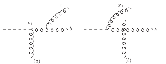
Figure 3: The real diagrams of deep inelastic scattering of the current off a large nucleus at one-loop order.

The coordinate variables are defined as $u_{\perp}=x_{\perp}-b_{\perp}$, $v_{\perp}=\xi x_{\perp}+(1-\xi)b_{\perp}$ and $u^{\prime}_{\perp}=x^{\prime}_{\perp}-b^{\prime}_{\perp}$, $v^{\prime}_{\perp}=\xi x^{\prime}_{\perp}+(1-\xi)b^{\prime}_{\perp}$, using these relationships, we can change the integral variables in the phase space integral, after some algebraic derivations, we get

$$\frac{\text{d}\sigma_{a}^{jA\to hX}}{\sigma_{0}\text{d}y\text{d}^{2}p_{h\perp}} = k^{+}\alpha_{s}N_{c}\int_{\tau}^{1}\frac{d\xi}{z^{2}_{1}}D(z_{1}/\xi)\frac{1}{\xi}\int\frac{\text{d}^{2}u_{\perp}}{(2\pi)^{2}}\frac{\text{d}^{2}v_{\perp}}{(2\pi)^{2}}\frac{\text{d}^{2}v^{\prime}_{\perp}}{(2\pi)^{2}}$$ (10)

$$\times e^{-ik_{\perp}\cdot(v_{\perp}-v^{\prime}_{\perp})}\sum\Psi^{\ast}_{g\to gg}\left(\xi,u^{\prime}_{\perp}\right)\Psi_{g\to gg}\left(\xi,u_{\perp}\right)S^{WW}(v_{\perp},v^{\prime}_{\perp}),$$

where $u_{\perp}^{\prime}=u_{\perp}-\frac{1}{\xi}(v_{\perp}-v^{\prime}_{\perp})=u_{\perp}-(x_{\perp}-x^{\prime}_{\perp})$, and we use $l_{1\perp}/k_{\perp}\approx l_{1}^{+}/k^{+}=\xi$. Substituting the sum of $\Psi_{g\to gg}(\xi,u_{\perp})$Dominguez:2011wm

$$\sum\Psi_{g\to gg}^{*}(\xi,u_{\perp}^{\prime})\Psi_{g\to gg}(\xi,u_{\perp})=(2\pi)^{2}\frac{4}{k^{+}}\left[\frac{\xi}{1-\xi}+\frac{1-\xi}{\xi}+\xi(1-\xi)\right]\frac{u_{\perp}^{\prime}\cdot u_{\perp}}{u_{\perp}^{\prime 2}u_{\perp}^{2}}$$ (11)

into Eq. (10), we get

$$\frac{\text{d}\sigma_{a}^{jA\to hX}}{\sigma_{0}\text{d}y\text{d}^{2}p_{h\perp}} = 4\alpha_{s}N_{c}\int\frac{\text{d}^{2}v_{\perp}\text{d}^{2}v^{\prime}_{\perp}}{(2\pi)^{2}}e^{-ik_{\perp}\cdot(v_{\perp}-v^{\prime}_{\perp})}S^{WW}(v_{\perp},v^{\prime}_{\perp})$$ (12)

$$\times\int_{\tau}^{1}\frac{d\xi}{z^{2}_{1}}D(z_{1}/\xi)\int\frac{\text{d}^{2}l_{2\perp}}{(2\pi)^{2}}e^{-il_{2\perp}\cdot\frac{1}{\xi}(v_{\perp}-v^{\prime}_{\perp})}\frac{1}{l_{2\perp}^{2}}\frac{1}{\xi}\left[\frac{1}{1-\xi}+\frac{1-\xi}{\xi}+\xi(1-\xi)\right].$$

We can see that the first line of Eq. (12) is proportional to the leading power differential cross section, which should be factorized out. The integral of the second line of Eq. (12) contains various types of divergences. In order to obtain the Sudakov logarithms terms, we should subtract these divergences. These divergences include rapidity divergence, collinear divergence, and other divergences. The rapidity divergence associates with the WW gluon distribution of the large nucleus targetDominguez:2011gc , and the collinear divergence associates with the fragmentation function of the final hadronChirilli:2011km , other divergences should be cancelled by virtual loops. It is necessary to subtract these divergences in order to obtain the Sudakov logarithms terms. Firstly, we can subtract the collinear divergence using the plus function. We can rewrite the second line of Eq. (12) as

$$\int_{\tau}^{1}\frac{d\xi}{z^{2}_{1}}D(z_{1}/\xi)\frac{\text{d}^{2}l_{2\perp}}{(2\pi)^{2}}e^{-il_{2\perp}\cdot R_{\perp}/\xi}$$

$$\times\frac{1}{l_{2\perp}^{2}\xi}\left[\frac{1}{(1-\xi)_{+}}+\frac{1-\xi}{\xi}+\xi(1-\xi)\right]$$

$$+\frac{D(z_{1})}{z^{2}_{1}}\int\frac{\text{d}^{2}l_{1\perp}}{(2\pi)^{2}}e^{-il_{2\perp}\cdot R_{\perp}}\frac{1}{l_{2\perp}^{2}}\int^{1}_{0}\text{d}\xi\frac{1}{1-\xi},$$ (13)

where $R_{\perp}=(v_{\perp}-v^{\prime}_{\perp})$, the first term of Eq. (13) can be interpreted as part of renormalization of the fragmentation function of final state hadron. We take $l_{2\perp}^{\prime}=l_{2\perp}/\xi$, and integrate it by $l_{2\perp}^{\prime}$, the integral of the first line is proportional to

$$\frac{1}{4\pi}\frac{1}{\xi}\left[\frac{\xi}{(1-\xi)}_{+}+\frac{1-\xi}{\xi}+\xi(1-\xi)\right]\left(-\frac{1}{\epsilon}+\ln\frac{c_{0}^{2}}{\mu^{2}R^{2}_{\perp}}\right),$$

(14)

where we use $\overline{MS}$ scheme, it is part of the splitting function. Then, we are going to calculate the integral of the second line of Eq. (13). According to momentum energy conversation, we can get the kinematics of graph $(a)$ in Fig. 3 as follows

$$x^{\prime}_{g}s=\frac{l^{2}_{2\perp}}{(1-\xi)}+\frac{l^{2}_{1\perp}}{\xi}.$$ (15)

In $\xi\rightarrow 1$ limit, we get

$$\xi<1-\frac{l^{2}_{2\perp}}{s}.$$ (16)

Now, the last integral of the second line of Eq. (13) can be written as

$$\int^{1-\frac{l^{2}_{2\perp}}{s}}_{0}\frac{1}{1-\xi}=\ln\frac{s}{l_{2\perp}^{2}}=\ln\frac{s}{Q^{2}}+\ln\frac{Q^{2}}{l_{2\perp}^{2}}$$ (17)

$$= \ln\frac{1}{x_{g}}+\ln\frac{Q^{2}}{l^{2}_{2\perp}}.$$

Back to Eq. (5), we get $x_{g}\to 0$, as $s\to\infty$, $\ln 1/x_{g}$ is divergent. In small-$x$ physics, the product of $\alpha_{s}$ and $\ln 1/x_{g}$ is resummed through the small-$x$ evolution equation of the WW gluon distribution. Thus the first logarithm term of Eq. (17) should be separated out from Sudakov resummation, and it should be absorbed into the renormalization of the WW gluon distributionDominguez:2011gc . The evolution equation of the WW gluon distribution is

$$\frac{\partial}{\partial\ln 1/x_{g}}S^{WW}(x_{\perp},x^{\prime}_{\perp})=\int{\bf K}_{\rm DMMX}\otimes S^{WW}(x_{\perp},x^{\prime}_{\perp}),$$

(18)

where ${\bf K}_{\rm DMMX}$ is the kernel of the small-$x$ evolution equation. Besides these two divergences, the integral of the second logarithm term of Eq. (17) contains other divergences, which can be cancelled by contributions of virtual loops, we can write the integral of the second logarithm term of Eq. (17) as

$$\mu^{2\epsilon}\int\frac{\text{d}^{2-2\epsilon}l_{2\perp}}{(2\pi)^{2-2\epsilon}}e^{-il_{2\perp}\cdot R_{\perp}}\frac{1}{l_{2\perp}^{2}}\ln\frac{Q^{2}}{l^{2}_{2\perp}},$$ (19)

where the integral dimension has been changed from $2$ to $2-2\epsilon$. Using the formulas in Appendix of Ref. Mueller:2013uf , we obtain the contribution of square of graph $(a)$ in Fig. 3

$$\frac{\alpha_{s}N_{c}}{\pi}\left(\frac{1}{\epsilon^{2}}-\frac{1}{\epsilon}\ln\frac{Q^{2}}{\mu^{2}}+\frac{1}{2}\ln^{2}\frac{Q^{2}}{\mu^{2}}-\frac{1}{2}\ln^{2}\frac{Q^{2}R_{\perp}^{2}}{c_{0}^{2}}-\frac{\pi^{2}}{12}\right),$$

(20)

where $c_{0}=2e^{-\gamma_{E}}$, $\gamma_{E}\approx 0.5772$ is Euler constant.
There are three kinds of virtual graphs in the DIS of current off a large nucleus as described in Fig. 4, the graph $(c)$ in Fig. 4 is the gluon self-energy diagram, the graph $(e)$ in Fig. 4 is the quark self-energy diagram. We begin with the calculation of the virtual graph $(d)$ in Fig. 4, and find

$$\frac{\text{d}\sigma_{d}^{jA\to hX}}{\sigma_{0}\text{d}y\text{d}^{2}p_{h\perp}} =-ik^{+}\alpha_{s}\frac{D(z_{1})}{z_{1}^{2}}\int_{0}^{1}\text{d}\xi\int\frac{\text{d}^{2}v_{\perp}}{(2\pi)^{2}}\frac{\text{d}^{2}v_{\perp}^{\prime}}{(2\pi)^{2}}\frac{\text{d}^{2}u_{\perp}}{(2\pi)^{2}}e^{-ik_{\perp}\cdot(v_{\perp}-v^{\prime}_{\perp})}\sum\Psi^{\ast}_{j\to gg}(\xi,u_{\perp})\Psi_{g\to gg}(\xi,u_{\perp})\{\text{Tr}U^{\dagger}(v^{\prime}_{\perp})$$

$$\times[\epsilon_{\perp}^{(1)}\cdot\partial U(v^{\prime}_{\perp})]U^{\dagger}(x_{\perp})U(b_{\perp})\text{Tr}U^{\dagger}(b_{\perp})U(x_{\perp})-\text{Tr}U^{\dagger}(v^{\prime}_{\perp})[\epsilon_{\perp}^{(1)}\cdot\partial U(v^{\prime}_{\perp})]U^{\dagger}(b_{\perp})U(x_{\perp})\text{Tr}U^{\dagger}(x_{\perp})U(b_{\perp})\}$$

$$+ik^{+}\alpha_{s}\frac{D(z_{1})}{z_{1}^{2}}\int_{0}^{1}\text{d}\xi\int\frac{\text{d}^{2}v_{\perp}}{(2\pi)^{2}}\frac{\text{d}^{2}v_{\perp}^{\prime}}{(2\pi)^{2}}\frac{\text{d}^{2}u^{\prime}_{\perp}}{(2\pi)^{2}}e^{-ik_{\perp}\cdot(v_{\perp}-v^{\prime}_{\perp})}\sum\Psi^{\ast}_{g\to gg}(\xi,u^{\prime}_{\perp})\Psi_{j\to gg}(\xi,u^{\prime}_{\perp})\{\text{Tr}U^{\dagger}(v_{\perp})$$

$$\times[\epsilon_{\perp}^{(1)\ast}\cdot\partial U(v_{\perp})]U^{\dagger}(x^{\prime}_{\perp})U(b^{\prime}_{\perp})\text{Tr}U^{\dagger}(b^{\prime}_{\perp})U(x^{\prime}_{\perp})-\text{Tr}U^{\dagger}(v_{\perp})[\epsilon_{\perp}^{(1)\ast}\cdot\partial U(v_{\perp})]U^{\dagger}(b^{\prime}_{\perp})U(x^{\prime}_{\perp})\text{Tr}U^{\dagger}(x^{\prime}_{\perp})U(b^{\prime}_{\perp})\}.$$

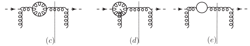
Figure 4: Virtual loop diagrams in the deep inelastic scattering of current off a large nucleus at one-loop order.

After lengthy calculations, where we only keep the leading power contribution, we get the contribution of graph $(d)$ in Fig. 4 after factoring out the leading order contribution,

$$\frac{\alpha_{s}N_{c}}{\pi}\left(-\frac{1}{\epsilon^{2}}+\frac{1}{\epsilon}\ln\frac{Q^{2}}{\mu^{2}}-\frac{1}{2}\ln^{2}\frac{Q^{2}}{\mu^{2}}+\frac{\pi^{2}}{12}\right).$$ (22)

We can see that $\pi^{2}/2$ in brackets is absent in Eq. (22) comparing to Eq. ($49$) of Ref. Mueller:2013uf since this process is space-like. Adding Eq. (20) and Eq. (22) together, we can get the Sudakov double logarithm term

$$-\frac{\alpha_{s}N_{c}}{2\pi}\ln^{2}\frac{Q^{2}R_{\perp}^{2}}{c_{0}^{2}}.$$ (23)

Next, we calculate the contributions of graph $(c)$ and graph $(e)$ in Fig. 4, the differential cross section of graphs $(c)$ in Fig. 4 can be cast into

$$\frac{\text{d}\sigma_{c}^{jA\to hX}}{\sigma_{0}\text{d}y\text{d}^{2}p_{h\perp}} = -\frac{1}{2}k^{+}\alpha_{s}N_{c}\frac{D(z_{1})}{z^{2}_{1}}\int_{0}^{1}\text{d}\xi$$ (24)

$$\times\int\frac{\text{d}^{2}v_{\perp}}{(2\pi)^{2}}\frac{\text{d}^{2}v_{\perp}^{\prime}}{(2\pi)^{2}}\frac{\text{d}^{2}u_{\perp}}{(2\pi)^{2}}e^{-ik_{\perp}\cdot(v_{\perp}-v^{\prime}_{\perp})}$$

$$\times\sum\Psi^{\ast}_{g\to gg}\left(\xi,u_{\perp}\right)\Psi_{g\to gg}\left(\xi,u_{\perp}\right)$$

$$\times S^{WW}(v_{\perp},v^{\prime}_{\perp}),$$

the differential cross section of graph $(e)$ in Fig. 4 can be cast into

$$\frac{\text{d}\sigma_{e}^{jA\to hX}}{\sigma_{0}\text{d}y\text{d}^{2}p_{h\perp}} = -k^{+}\alpha_{s}T_{f}N_{f}\frac{D(z_{1})}{z_{1}^{2}}\int_{0}^{1}\text{d}\xi$$ (25)

$$\times\int\frac{\text{d}^{2}v_{\perp}}{(2\pi)^{2}}\frac{\text{d}^{2}v_{\perp}^{\prime}}{(2\pi)^{2}}\frac{\text{d}^{2}u_{\perp}}{(2\pi)^{2}}e^{-ik_{\perp}\cdot(v_{\perp}-v^{\prime}_{\perp})}$$

$$\times\sum\Psi^{\ast}_{g\to q\bar{q}}\left(\xi,u_{\perp}\right)\Psi_{g\to q\bar{q}}\left(\xi,u_{\perp}\right)$$

$$\times S^{WW}(v_{\perp},v^{\prime}_{\perp}),$$

where $N_{f}$ is the number of quark flavors and $T_{f}=\frac{1}{2}$. The splitting function of $\Psi_{g\to q\bar{q}}\left(\xi,u_{\perp}\right)$ can be found in Ref. Dominguez:2011wm ; Chirilli:2011km and the sum of the splitting function is

$$\sum \Psi^{\ast}_{g\to q\bar{q}}\left(\xi,u_{\perp}\right)\Psi_{g\to q\bar{q}}\left(\xi,u_{\perp}\right)$$ (26)

$$=\frac{2}{k^{+}}(2\pi)^{2}\left[\xi^{2}+(1-\xi)^{2}\right]\frac{1}{u_{\perp}^{2}}.$$

The sum of graph $(c)$ and $(d)$ in Fig. 4 gives

$$-\frac{\alpha_{a}N_{c}}{\pi}\left[\beta_{0}\left(-\frac{1}{\epsilon_{\textrm{IR}}}+\ln\frac{Q^{2}}{\mu^{2}}\right)+\beta_{0}\left(\frac{1}{\epsilon_{\textrm{UV}}}-\ln\frac{Q^{2}}{\mu^{2}}\right)\right],$$

(27)

where $\beta_{0}$ is $(11-2N_{f})/12N_{c}$. We can see that there are two divergences in Eq. (27), infrared divergence and Ultraviolet divergence, they should be subtracted in Sudakov resummation. The term of Ultraviolet divergence

$$-\frac{\alpha_{a}N_{c}}{\pi}\beta_{0}\left(\frac{1}{\epsilon_{\textrm{UV}}}-\ln\frac{Q^{2}}{\mu^{2}}\right)$$ (28)

is absorbed into the renormalization of the coupling constant $\alpha_{s}$. The infrared divergence and the contribution of Eq. (14) are absorbed into the fragmentation function of the final state hadronChirilli:2011km as follows

$$D_{h/g}(z_{1},\mu)=D^{(0)}_{h/g}(z_{1})-\frac{1}{\epsilon}\frac{\alpha_{s}N_{c}}{\pi}\int_{z_{1}}^{1}\frac{d\xi}{\xi}\mathcal{P}(\xi)_{gg}D_{h/g}(\frac{z_{1}}{\xi}),$$

where

$$\mathcal{P}_{gg}(\xi)=\frac{\xi}{(1-\xi)_{+}}+\frac{1-\xi}{\xi}+\xi(1-\xi)+\beta_{0}\delta(1-\xi).$$ (30)

After subtracting these two divergences, we can get the single logarithm term of the Sudakov factor as follows

$$\frac{\alpha_{s}N_{c}}{\pi}\beta_{0}\ln\frac{Q^{2}R_{\perp}^{2}}{c_{0}^{2}},$$ (31)

where we set the factorization scale $\mu^{2}=c_{0}^{2}/R_{\perp}^{2}$. Adding the double and single logarithms terms together, we get the Sudakov factor of DIS of a current off a large nucleus at one-loop order

$${\cal S}_{\textrm{sud}}(Q^{2},R_{\perp}^{2})=\frac{\alpha_{s}N_{c}}{\pi}\left(\beta_{0}\ln\frac{Q^{2}R_{\perp}^{2}}{c_{0}^{2}}-\frac{1}{2}\ln^{2}\frac{Q^{2}R_{\perp}^{2}}{c_{0}^{2}}\right).$$

(32)

At the end of the day, assuming the exponentiation of one-loop result, we can write down the differential cross section of DIS of a gluonic current off a large nucleus at one-loop order including Sudakov factor as

$$\frac{d\sigma^{\rm({\rm resum})}}{\sigma_{0}dyd^{2}p_{h\perp}}|_{k^{2}_{\perp}\ll Q^{2}} = \frac{D_{h/g}(z_{1})}{z^{2}_{1}}\int\frac{d^{2}v_{\perp}d^{2}v_{\perp}^{\prime}}{(2\pi)^{2}}e^{ik_{\perp}\cdot(v_{\perp}-v^{\prime}_{\perp})}$$

$$\times e^{-{\cal S}_{\textrm{sud}}(Q^{2},R_{\perp}^{2})}S^{WW}_{Y=\ln 1/x_{g}}(v_{\perp},v_{\perp}^{\prime}).$$

IV photon pair production in $pA$ collisions

Two kinds of gluon distributions are introduced in Ref. Dominguez:2011wm . The first gluon distribution is WW gluon distribution which we have mentioned, the second one is dipole gluon distribution, which is fourier transform of the dipole cross section. They are different in many ways, the WW gluon distribution only contains initial or final interaction, the dipole gluon distribution contains both initial and final interaction. The WW gluon distribution can be interpreted as the number density of gluons in the light-cone gauge, but the diploe gluon distribution has no such interpretation. They appear in different physics processes.
Let’s consider the process of $pA\rightarrow\gamma\gamma+X$, which is described in Fig. 5, The left graph in Fig. 5 is the feynman diagram at leading-order , the right graph in Fig. 5 is the feynman diagram at one-loop order, there are five other feynman diagrams similar to each diagram, and they are omitted. $k_{1}$ and $k_{2}$ are the momentum of the two observed photons, $q_{p}$ is the momentum of the incoming gluon from proton, $p_{A}$ is the momentum of the outgoing gluons from nucleus target. As we see from the feynman diagram, there is only initial interaction in the process of $pA\rightarrow\gamma\gamma+X$, thus, the involving gluon distribution is WW gluon distribution. In this process, we assume that the observed two photons are radiated back-to-back, and have large transverse momentum.

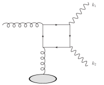
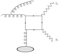
Figure 5: Feynman diagrams of $pA\rightarrow\gamma\gamma+X$, the left one is the leading-order contribution, the right one is the real contribution at one-loop order.

We define $q_{\perp}=|k_{1\perp}+k_{2\perp}|$ and $P_{\perp}=|k_{1\perp}-k_{2\perp}|/2$, and assume that $P_{\perp}\simeq|k_{1\perp}|\simeq|k_{2\perp}|\gg q_{\perp}=|k_{1\perp}+k_{2\perp}|$. Thus, we should only keep the contribution which is not suppressed by term of $q_{\perp}^{2}/P_{\perp}^{2}$ when we are calculating the Sudakov factor for this process.
Following the same strategy as in Ref. Dominguez:2011wm , we can compute the Sudakov contribution at the one-loop order. Eventually, the differential cross section of $pA\to\gamma\gamma+X$ can be cast into

$$\frac{\text{d}\sigma^{pA\rightarrow\gamma\gamma+X}}{\text{d}y_{1}\text{d}y_{2}\text{d}^{2}P_{\perp}\text{d}^{2}q_{\perp}} = x_{p}f(x_{p})\frac{2}{\pi\alpha_{s}}\frac{\text{d}\sigma^{gg\rightarrow\gamma\gamma}}{\text{d}t}\int\frac{d^{2}x_{\perp}}{(2\pi)^{2}}\frac{d^{2}x^{\prime}_{\perp}}{(2\pi)^{2}}$$ (34)

$$\times e^{iq_{\perp}\cdot(x_{\perp}-x^{\prime}_{\perp})}S^{WW}(x_{\perp},x_{\perp}^{\prime})$$

$$\times e^{-{\cal S}_{\textrm{sud}}(P_{\perp}^{2},R_{\perp})}$$

where $y_{1}$ and $y_{2}$ are the rapidities of the two outgoing photons, the $x_{p}f(x_{p})$ is the collinear gluon distribution of the proton. $\text{d}\sigma^{gg\rightarrow\gamma\gamma}/\text{d}t$ is the hard part of $gg\rightarrow\gamma\gamma$Berger:1983yi ; Dicus:1987fk ; Bern:2001df , the explicit expression of the hard part can be found in Table 2 of Ref. Berger:1983yi . The Sudakov double logarithm in this process is the same as the one of Higgs production in $pA$ collisions, which is

$${\cal S}_{\textrm{sud}}(P_{\perp}^{2},R_{\perp})=\frac{\alpha_{s}N_{c}}{2\pi}\ln^{2}\frac{P_{\perp}^{2}R_{\perp}^{2}}{c^{2}_{0}},$$ (35)

when we calculate the Sudakov double logarithms term.
In this process, we only keep $x_{g}$ small. Since $x_{p}x_{g}s\approx P_{\perp}^{2}$, $x_{p}$ is large, thus, $x_{p}f(x_{p})$ can be obtained by database. If the differential cross section of $pA\rightarrow\gamma\gamma+X$ is measured by experiment, we can gain the information of the WW gluon distribution $S^{WW}(x_{\perp},x_{\perp}^{\prime})$. It is an interesting way to study the WW gluon distribution at the LHC and RHIC.
There is another channel of the photon pair production in $pA$ collisions, the incoming particles from the proton and nucleus are not gluons, but quark and antiquark, the hard part of the channel is $\mathcal{H}_{q\bar{q}\rightarrow\gamma\gamma}$. When the scattering energy is high, the quark and antiquark distributions are much smaller than the gluon distributions, thus, the channel of $q\bar{q}\rightarrow\gamma\gamma$ can be neglected in photon pair production in $pA$ collisions.

V conclusion

In summary, we consider two physics processes involving WW gluon distribution. The first process is the DIS of current off a large nucleus, and the second one is the photon pair production in $pA$ collisions. The WW gluon distribution in the DIS of current off a large nucleus only contains final interaction, the WW gluon distribution of the photon pair production in $pA$ collisions only contains initial interaction.
Based on the leading power approximation, we have calculated the Sudakov factor in DIS of gluoic current off a large nucleus at one-loop order. The contributions from many real and virtual graphs are power suppressed under the leading power approximation, and they are neglected in the calculation. In the calculation, we find that there are various types of divergences at one-loop order, the divergences must be separated out from the Sudakov resummation. The collinear divergence is absorbed into renormalization of the fragmentation function of the final state hadron, the rapidity divergence is absorbed into the renormalization of the WW gluon distribution, the UV divergence is absorbed into the renormalization of coupling constant. After subtracting the divergences, we get Sudakov factor which include double and single logarithms terms. Finally, we get differential cross section of DIS of gluonic current off a large nucleus including the Sudakov factor at one-loop order.
We also consider the process of photon pair production in $pA$ collisions, where the final interaction is absent in this process. Thus, the involving gluon distribution is the WW gluon distribution. Based on the TMD-factorization, we get differential cross section expression including the Sudakov factor at one-loop order. It is suggested that if the differential cross section is measured at the LHC and RHIC, the WW gluon distribution $S^{WW}(x_{\perp},x_{\perp}^{\prime})$ may be extracted from the experimental data.

References

• (1) L. V. Gribov, E. M. Levin and M. G. Ryskin, Phys. Rept.  100, 1 (1983).
• (2) A. H. Mueller, Nucl. Phys. B 335, 115 (1990); A. H. Mueller, hep-ph/0111244.
• (3) I. I. Balitsky and L. N. Lipatov, Sov. J. Nucl. Phys.  28, 822 (1978) [Yad. Fiz.  28, 1597 (1978)].
• (4) E. A. Kuraev, L. N. Lipatov and V. S. Fadin, Sov. Phys. JETP 45, 199 (1977) [Zh. Eksp. Teor. Fiz.  72, 377 (1977)]; A. H. Mueller, Nucl. Phys. B 415, 373 (1994).
• (5) A. H. Mueller and J. W. Qiu, Nucl. Phys. B 268, 427 (1986).
• (6) I. Balitsky, Nucl. Phys. B 463, 99 (1996); Y. V. Kovchegov, Phys. Rev. D 60, 034008 (1999).
• (7) J. Jalilian-Marian, A. Kovner, A. Leonidov and H. Weigert, Nucl. Phys. B 504, 415 (1997); Phys. Rev. D 59, 014014 (1998).
• (8) E. Iancu, A. Leonidov and L. D. McLerran, Nucl. Phys. A 692, 583 (2001); Nucl. Phys. A 703, 489 (2002); hep-ph/0202270.
• (9) V. V. Sudakov, Sov. Phys. JETP 3, 65 (1956) [Zh. Eksp. Teor. Fiz.  30, 87 (1956)].
• (10) J. C. Collins, D. E. Soper and G. F. Sterman, Nucl. Phys. B 250, 199 (1985).
• (11) C. T. H. Davies, B. R. Webber and W. J. Stirling, Nucl. Phys. B 256, 413 (1985).
• (12) A. H. Mueller, B. -W. Xiao and F. Yuan, Phys. Rev. Lett.  110, 082301 (2013).
• (13) A. H. Mueller, B. -W. Xiao and F. Yuan, Phys. Rev. D 88, 114010 (2013).
• (14) J. C. Collins and D. E. Soper, Nucl. Phys. B 194, 445 (1982).
• (15) L. D. McLerran and R. Venugopalan, Phys. Rev. D 49, 2233 (1994); Phys. Rev. D 49, 2233 (1994).
• (16) X. -d. Ji, J. -P. Ma and F. Yuan, JHEP 0507, 020 (2005).
• (17) F. Dominguez, A. H. Mueller, S. Munier and B. -W. Xiao, Phys. Lett. B 705, 106 (2011).
• (18) Y. V. Kovchegov and A. H. Mueller, Nucl. Phys. B 529, 451 (1998).
• (19) F. Dominguez, C. Marquet, B. W. Xiao and F. Yuan, Phys. Rev. D 83, 105005 (2011).
• (20) A. H. Mueller, Nucl. Phys. B 558, 285 (1999).
• (21) G. A. Chirilli, B. -W. Xiao and F. Yuan, Phys. Rev. Lett.  108, 122301 (2012); Phys. Rev. D.  86, 054005 (2012).
• (22) E. L. Berger, E. Braaten and R. D. Field, Nucl. Phys. B 239, 52 (1984).
• (23) D. A. Dicus and S. S. D. Willenbrock, Phys. Rev.  D 37, 1801 (1988).
• (24) Z. Bern, A. De Freitas and L. J. Dixon, JHEP 0109, 037 (2001).