Origin of the peculiar eccentricity distribution of the inner cold Kuiper belt

Abstract

Dawson and Murray-Clay (2012) pointed out that the inner part of the cold population in the Kuiper belt (that with semi major axis $a<43.5$ AU) has orbital eccentricities significantly smaller than the limit imposed by stability constraints. Here, we confirm their result by looking at the orbital distribution and stability properties in proper element space. We show that the observed distribution could have been produced by the slow sweeping of the 4/7 mean motion resonance with Neptune that accompanied the end of Neptune’s migration process. The orbital distribution of the hot Kuiper belt is not significantly affected in this process, for the reasons discussed in the main text. Therefore, the peculiar eccentricity distribution of the inner cold population can not be unequivocally interpreted as evidence that the cold population formed in-situ and was only moderately excited in eccentricity; it can simply be the signature of Neptune’s radial motion, starting from a moderately eccentric orbit. We discuss how this agrees with a scenario of giant planet evolution following a dynamical instability and, possibly, with the radial transport of the cold population.

1 Introduction

The Kuiper belt has a complex orbital structure and can be divided in multiple sub-populations (see Gladman et al., 2008 for a review). Among them are the cold and the hot populations, which are defined as the collections of objects inwards of the 1/2 resonance with Neptune ($\sim 48$ AU) with, respectively, inclinations smaller or larger than 4 degrees. The cold and hot populations have also distinct physical properties (see Morbidelli and Brown, 2004 for a review).

There is a quite general consensus that the hot population formed originally closer to the Sun, was dynamically excited by the perturbations from the giant planets and finally was transported into the Kuiper belt (Gomes, 2003; Levison et al., 2008). However, there is no consensus on the origin of the cold population. Some models argue that it also was transported into the Kuiper belt from a region closer to the Sun (Levison and Morbidelli, 2003; Levison et al., 2008), while others argue that the cold population formed locally (e.g. Parker et al., 2011; Batygin et al., 2011).

An important point in this debate was made by Dawson and Murray-Clay (2012). First they observed that the usual partition of the cold and hot populations according to the 4-degree inclination boundary is simplistic; in reality these populations have distinct, but partially overlapping inclination distributions (see Brown, 2001). Thus, to limit the contamination of the cold population by the hot population, they restricted their analysis to objects with inclination $i<2^{\circ}$, where the relative fraction of low-inclination “hot” objects is expected to be negligible. Then they showed that, inside of 43.5 AU, this low-inclination population has also small eccentricities ($e\lesssim 0.05$), even though orbits would be stable up to $e\sim 0.1$ (Lykawka and Mukai, 2005a). The hot population, in fact, has eccentricities up to this limit. The lack of moderate eccentricity orbits in the cold population obviously cannot be explained by observational biases. Dawson and Murray-Clay therefore interpreted this result as evidence that the cold Kuiper belt was only very moderately excited relative to its original quasi-circular and coplanar orbits. This argues against models in which the cold population originates closer to the sun and is implanted into the Kuiper belt, because such models predict a cold population with an eccentricity distributions covering the whole stability range.

Given the importance of this argument, we have decided to revisit the problem of the eccentricity distribution of the cold Kuiper belt. In Section 2 we redo the same analysis as Dawson and Murray-Clay, but using proper elements instead of osculating elements. Our results confirm theirs, but we notice that the transition between the inner part of the cold population, where eccentricities are all small, to the outer part, where the eccentricities cover a wider range, happens exactly at the 4/7 mean motion resonance with Neptune. This suggests that this resonance might have played a role in sculpting the inner cold belt during a phase of outward migration. Then, in Section 3 we conduct migration experiments, testing different migration timescales and eccentricities of Neptune. Section 4 analyzes more in details how moderate-eccentricity cold Kuiper belt objects are removed by resonance sweeping and compares their evolution with that of high inclination bodies. Our conclusions are discussed in Section 5.

2 Distribution of proper elements and stability map for the cold Kuiper belt

We have selected all TNOs from the MPC catalog with semi major axis larger than 25 AU and orbits determined from observations covering at least three oppositions. Such procedure selected a set of 811 TNOs. For each of these objects we computed numerically the orbital proper elements using integrations covering 132 My. The proper semi major axis was computed by numerical average of the values recorded during the simulation, with an output time-step of 1,000y. For the proper eccentricities and inclinations, the computational procedure was more elaborated, although standard (Knezevic and Milani, 2000). We first computed the Fourier series of $(h(t),k(t))$ and $(p(t),q(t))$, where:

$$h(t) = e(t)\cos[\varpi(t)]$$ (1)

$$k(t)) = e(t)\sin[\varpi(t)]$$ (2)

$$p(t) = i(t)\cos[\Omega(t)]$$ (3)

$$q(t)) = i(t)\sin[\Omega(t)]$$ (4)

and $e(t),i(t),\varpi(t)$ and $\Omega(t)$ are the values of eccentricity, inclination, longitude of perihelion and longitude of node recorded over time $t$. We then removed from the series expansions the terms with frequencies close (i.e. within one arcsec/y) to the proper frequencies of the planets. Finally, we selected as proper eccentricity and inclination the coefficients of the largest remaining term in the each of the two Fourier series.

In order to evaluate the accuracy of proper eccentricity and inclination, we performed the procedure described above for the first and the second halves of the whole integration, i.e., 65.536 My. Then, we adopted as an estimate of the error, the largest difference among the proper elements calculated for the whole integration time-span and those computed in each of the two half time-spans. The relative accuracy in proper semi major axis was always better than $3\times 10^{-4}$. The absolute accuracies in proper eccentricity and inclinations were better than 0.01 and 0.1 degrees throughout the region of interest (i.e. inside of 44 AU and not in the 4/7 mean motion resonance with Neptune).

Once in possession of this proper element catalog, following Dawson and Murray-Clay we retained as members of an “uncontaminated cold population” the objects with proper inclination smaller than 2 degrees. Fig. 1 shows the distribution of the selected objects (dots) in proper semi major axis vs. eccentricity plane.

We also computed a new stability map. In fact, the map used by Dawson and Murray-Clay, from Lykawka and Mukai (2005a), was computed for a wide range of inclinations, whereas here we are interested to very low inclinations only. We could have used the stability map in Duncan et al. (1995), which was computed for $i=1^{\circ}$, but the latter was quite sparse, due to the computing limitations of the time. Moreover, both Lykawka and Mukai and Duncan et al. reported their maps relative to the initial osculating elements. Here, for a consistent comparison with the proper elements of the real objects, we needed a map computed in proper elements space.

To compute the stability map, we proceeded as follows. We adopted a grid of particles’ initial conditions, with osculating elements in the following ranges: 42 AU $<a<$ 48 AU, $0<e<0.2$ and $0<i<2$ deg, with resolutions of 0.2 AU in $a$, 0.01 in $e$ and 0.5 degrees in $i$. The secular angles $\Omega$ and $\varpi$ were set equal to 0 degrees. Each particle was integrated for 132 My. We then computed their proper elements following the same procedure described above. Finally, we continued the simulations for 4 Gy in order to asses the long-term survival of the test particles.

To construct Fig. 1, for each given pair of initial $a$ and $e$, we selected the particle with the smallest value of proper inclination. Then, for the particles that survived in the 4 Gy integration (i.e. they did not encounter Neptune within a Hill radius within this time), we plotted on a white background a light-gray square of size 0.2 AU$\times 0.01$ centered on their values of proper semi major axis and eccentricity measured on the first 132 My. Moreover, particles that did not survive were denoted by dark-gray squares centered on the initial pair of osculating semi major axis and eccentricity.

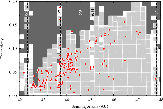
Figure 1: The dots show the distribution of proper semi major axis and proper eccentricities of the Kuiper belt objects with well-defined orbits and proper inclination smaller than 2 degrees. The light-gray squares denote the regions of proper element space that are stable in 4 Gy simulations and the dark-gray squares denote the initial orbital elements of unstable particles. White color is the background. The light-gray squares are not regularly spaced because the application mapping the initial conditions (regularly spaced) to proper elements is not linear. The vertical dashed lines depict the main mean motion resonances as labeled.

The stability map of Fig. 1 shows few surprises. In general, particles are unstable at large eccentricity and stable at low eccentricity, where the perihelion distance is larger than $\sim 38$–40 AU. Mean motion resonances represent the exception to this general rule. The light-gray squares at large eccentricity are all associated to mean motion resonances, as well as the vertical white columns at low or moderate eccentricities. Some mean motion resonances, therefore, clearly stand out from the stability map, and they are labelled on the figure.

In general, as expected, the dots fall on light-gray squares. Those that don’t, are associated to mean motion resonances. In fact, in a mean motion resonance there is a third dimension characterizing the orbit: the resonant amplitude. It is well possible that none of the test particles that we used for the stability map sampled the orbit of a real particle because their libration amplitude is different. In this case, a dot is plotted over the white background.

Overall, Fig. 1 confirms the results of Dawson and Murray-Clay. Inside of 43.5 AU, all real objects have small eccentricities, barely exceeding 0.05. The stability map, however, ranges up to 0.1 in the 42.2-42.6 AU region. Thus, there is clearly a stable region (approximately in the range $0.05<e<0.1$) in the inner belt that is not inhabited by the cold population. At a closer inspection, one sees that the transition in eccentricity distribution of the cold belt is sharply at the location of the 4/7 resonance (see Lykawka and Mukai, 2005b for a description of this resonance).

This result suggests that the 4/7 resonance might have played a role in depleting the moderate-eccentricity cold objects inside of its current location, as it swept through the 42.5–43.5 AU region during the putative radial migration of Neptune. Thus, in the following section, we report on numerical experiments of radial migration that address whether this is indeed possible and at which conditions.

3 Migration numerical experiments: the role of the 4/7 resonance sweeping

We set up simple numerical experiments, where Jupiter, Saturn and Uranus were assumed to be on their current orbits, while Neptune’s mean semi major axis was forced to change from $a_{i}=28.5$ AU to its current average value $a_{c}=30.1$AU as

$$a(t)=a_{c}+(a_{i}-a_{c})\times\exp(-t/\tau)$$

. The eccentricity of Neptune was also damped from an initial value $e_{0}$ as

$$\frac{1}{e}\frac{{\rm d}e}{{\rm d}t}=\alpha\exp(-t/\tau)$$

with an appropriate coefficient $\alpha$ that allowed us to match the current eccentricity of Neptune at the end of the simulation. Each simulation was run for a time-span of $6\times\tau$. The semi major axis drift and the eccentricity damping were implemented by applying synthetic forces to Neptune’s equations of motion. In particular, we employed the forces described in Malhotra (1995) for evolving the semi-major axes and those in Kominami et al. (2005) for controlling the eccentricity.

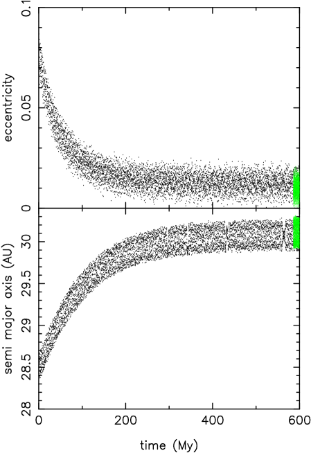
Figure 2: The evolution of Neptune during the migration experiment with $\tau=100$ my and $e_{0}=0.1$. The top panel depicts the time evolution of the eccentricity and the bottom panel that of the semi major axis. The green area close to the $t=600My$ axis is obtained by plotting the evolution of Neptune in the current solar system, and represents the target $a$ and $e$ that a good migration simulation needs to hit.

Fig. 2 shows the evolution of Neptune in a simulation with $\tau=100$ My and $e_{0}=0.1$. Notice that, although the initial eccentricity is 0.1, the mean eccentricity at the beginning of the simulation is only 0.075. The green area at the right-hand-side of each panel shows the current range of oscillations of the semi major axis and eccentricity of Neptune in the real Solar System. This shows that our migration evolution reproduces the actual orbit of Neptune with a good accuracy.

Overall we did 9 simulations, corresponding to the values of $\tau$ and $e_{0}$ reported in Table 1. These values cover a range of proposed migration models, with and without a putative initial eccentricity excitation of Neptune’s orbit. We will discuss in Sect. 5 what the successful parameters imply for the history of the Solar System. In each simulation we considered a population of 1,000 test particles, initially spread in osculating elements between 42.3 and 44.2 AU (in some cases only up to 43.6 AU) in semi major axis, from 0 to 0.15 in eccentricity and up to 2 degrees in inclination (with a uniform distribution in $\sin(i)$). Particles got discarded when they had encounters with Neptune. For the surviving particles we computed the proper elements over the final part of the simulation. Only particles with final proper inclination smaller than 2 degrees were considered.

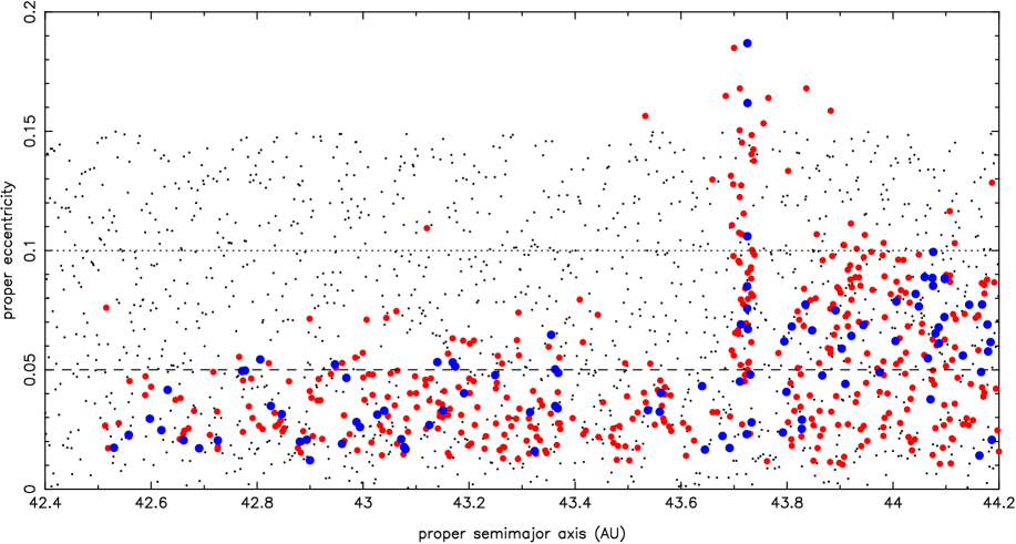
Figure 3: Comparison between the real distribution and the simulated distribution at the end of the simulation with $\tau=100$ My and $e_{0}=0.1$. The red dots depict the simulated particles and the blue dots the real cold belt objects (the same as shown in Fig. 1). The column of objects at $a\sim 43.72$ AU marks the location of the 4/7 resonance with Neptune. The small black dots depict the initial conditions of the simulated particles. Horizontal lines at $e=0.1$ and $e=0.05$ are plotted for reference.

Fig. 3 shows the final particle distribution (red dots) obtained in the simulation with $\tau=100$ My and $e_{0}=0.1$. Their final proper semi major axes have been multiplied by a factor 1.00092, to compensate for the slight offset of the final semi major axis of Neptune relative to the real one, visible in Fig. 2. For comparison, the blue dots represent the real low-inclination cold population (the same as in Fig. 1) and the small black dots show the initial conditions.

First, notice the cluster of simulated particles in the 4/7 resonance at $\sim 43.72AU$. This cluster is visible in the observations as well, in the right proportion. In fact, the ratio between the number of resonant particles and that of particles with $a<43.6$ AU is 26.3% at the end of the simulation; among observed objects, this ratio is 25.6%. Obviously, one has to take into account that observational biases may act differently on resonant and non-resonant objects, so that this agreement may just be accidental. However, we argue that in this case the differential bias effect is probably not a big issue. In fact, both resonant and non-resonant objects considered here have small inclinations and eccentricities; moreover objects in the 4/7 resonance can reach perihelion at 4 different position in the sky relative to Neptune, so that it is unlikely that all these sweet-spots have been missed by the surveys.

Second, notice that inside of the final location of the 4/7 resonance, most of the particles with moderate eccentricities have been removed. Thus, the final distribution is strongly skewed towards small eccentricities, more or less similar to the observed distribution.

Table 1: A summary of the results of the statistical tests for 9 simulations. The first line reports the value of $\tau$ and the first column that of $e_{0}$ (in parenthesis the initial mean value for $e$). Each case of the matrix reports $P_{1}/P_{2}/P_{1+2}$, where $P_{1}$ is the probability that criterion 1 is fulfilled, $P_{2}$ is the probability for criterion 2 and $P_{1+2}$ is the probability that both criteria are fulfilled simultaneously. See text for definition of criteria.

${}_{e_{0}}\setminus{}^{\tau}$	100 My	30 My	10 My
0.05 (0.036)	0.035 / 0.18 / 0.015	0.0004 / 0.0099 / 0.0001	0.0008 / 0.018 / 0.0005
0.1 (0.075)	0.18 / 0.80 / 0.17	0.0019 / 0.0062 / 0.0003	0.0 / 0.0008 / 0.0
0.15 (0.14)	unstable	unstable	unstable

Notice also that, beyond 43.8 AU, a similar truncation in the particle distribution occurs, but at proper $e=0.1$. Remember that Fig. 1 shows that, in the current Solar System, orbits in this region would be stable up to $e\sim 0.14$. The truncation at $e=0.1$ is also visible in the observed distribution and in our simulation is operated by the 5/9 resonance sweeping. Resonant sweeping, however, can not explain the “wedge”, namely the paucity of low eccentricity objects ($e<0.05$) beyond 43.8 AU; therefore, some other explanation is needed (e.g. Batygin et al., 2011) for this structure.

In order to quantify how well the simulated distribution reproduces the observed distribution we proceeded as follows. We considered objects and test particles in the 42.4–43.6 range only. The observed distribution in this range is made of 43 objects. The object with the largest proper eccentricity has $e=0.0653$. In total, there are only 7 objects with proper $e>0.05$. The simulated distribution has 194 test particles. In this count, we discarded the two particles with proper eccentricity larger than 0.1 because, from the stability map in Fig. 1, we know that these particles are unstable on the long term. We then did a Monte Carlo simulation. From the simulated distribution, we generated 10,000 synthetic populations, each of which contained 43 particles (the same number as that of the objects in the observed population). We considered two criteria of “success”. The first was that a synthetic population contained no particles with proper eccentricity larger than 0.0653 (criterion 1); the second was that the population contained no more than 7 particles with proper $e>0.05$ (criterion 2). We found that 18% of the synthetic populations fulfilled criterion 1; 80% of them fulfilled criterion 2 and 17% fulfilled simultaneously criterion 1 and 2. From this test, therefore, we conclude that the simulated population is statistically equivalent to the observed population (in the sense that it cannot be rejected even at a $1-\sigma$ level). Thus, we conclude that the slow migration of the 4/7 resonance with an initial moderate eccentricity of Neptune can explain the properties of the inner part of the cold population of the Kuiper Belt.

The results of the same statistical tests for the other simulations are reported in Table 1. As one can appreciate, fast migrations with $\tau=10$ or 30 My do a poor job in reproducing the observations. The simulation with $\tau=100My$ and $e_{0}=0.05$ does a decent job if one considers criterion 2, but it is consistent with the observed population only at the $2-\sigma$ level if one considers criterion 1. If one considers both criteria simultaneously, the simulated population has only a 1% chance to match the observed population. So, both the migration speed and the initial eccentricity of Neptune are important (see Sect. 4 for an explanation of this result). However, if Neptune is too eccentric (e.g. in the simulations with $e_{0}=0.15$) the entire inner Kuiper belt is destabilized, as described in Levison et al. (2008) and almost no particles survive with proper $i<2^{\circ}$ in the considered semi major axis range.

All these results do not depend strictly on the adopted $i<2^{\circ}$ limit; they would basically be the same for any reasonable boundary in proper inclination.

4 Comparative evolutions of the Hot and Cold populations

Our proposed explanation for the peculiar orbital structure of the cold population would not be acceptable without showing that the hot population avoids being sculpted in a similar fashion by the same process. In fact, as shown by Dawson and Murray-Clay (2012), the hot population does not exhibit any apparent deficit of objects with $e>0.05$.

For this purpose, we run again our best-case simulation, that with $\tau=100$ My and $e_{0}$=0.1, with a population of test particles having the following initial osculating orbital elements: $2^{\circ}<i<30^{\circ}$, 42.3 AU $<a<$ 43.6 AU, and $e<0.15$. The initial conditions and the proper elements of the surviving population are shown in Fig. 4.

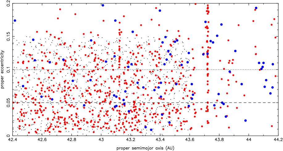
Figure 4: The same as Fig. 3 but for test particles initially with $a<43.6$ AU and $i>2^{\circ}$ and observed KBOs with current inclination larger than 4 degrees. Notice that the depletion of test particles with $e>0.05$ is much less pronounced than for the low-inclination population.

It can be immediately appreciated that the depletion of particles with eccentricity above 0.05 is much less effective than for the cold population. Thus, the hot population should have preserved its original (i.e. post-capture) eccentricity distribution. For this reason, and given the simple initial distribution (uniform) of our particles, the simulated final distribution is not intended to match the observations, but just to demonstrate that a moderate-eccentricity hot population could have survived the same migration scenario that explains the removal of the moderate-eccentricity cold population.

The differences between Fig. 3 and 4 is so striking that it calls for an explanation. To understand what happens, we looked at the individual evolution of particles in both simulations. A representative evolution of particles removed at low inclination is shown in Figs. 5 and that of particles surviving at high inclination is shown in Fig. 6. Each figure shows the behavior of semi major axis (bottom panel) and eccentricity (top panel) over time, while depicting also the evolving location of the 4/7 and 5/9 resonances with Neptune. Notice that both particles have initially comparable values of semi major axis and eccentricity. The low inclination particle has $i=0.5^{\circ}$ and the high inclination particle has $i=19^{\circ}$.

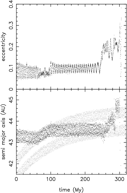
Figure 5: The evolution of a low inclination particle. The top panel depicts the time evolution of the eccentricity and the bottom panel that of the semi major axis (black dots). The gray dots show the semi major axis of Neptune rescaled by the factors $(9/5)^{2/3}$ and $(7/4)^{(}2/3)$, namely they depict the locations of the 5/9 and 4/7 resonances.

Fig. 5 shows that the low-inclination particle was captured in mean motion resonance with Neptune twice. First, the particle was captured in the 5/9 resonance, between 60 and 100 My. This is clear from the drift in particle’s semi major axis along the resonant track. Then the particle was released and it was captured in the 4/7 resonance at $t\sim 245$ My. This was a brief capture episode, but enough to raise the the eccentricity up to 0.2. Thus, the particle was destabilized: it was scattered by Neptune until it was dynamically removed. This shows that the cold population with moderate eccentricities was not lifted to into the hot population, but rather it was removed into the scattered disk.

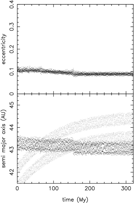
Figure 6: The same as Fig. 5 but for a high inclination particle.

Fig. 6, shows a completely different behavior: the high-inclination particle crossed both resonances without being captured. The semi major axis and the eccentricity show a distinctive jump each time that a resonance was crossed, but the eccentricity was not significantly affected overall. Thus, the particle remained stable till the end of the simulation.

Why is the probability of capture into resonance so different for low inclination and high inclination particles? We argue that the explanation is in the resonant structure. At small inclination, a mean motion resonance can be approximated by an integrable single-harmonic Hamiltonian. For the 4/7 resonance the harmonic term is $e^{3}\cos(4\lambda_{N}-7\lambda+3\varpi)$ where $\lambda$ and $\lambda_{N}$ are the mean longitudes of the particle and of Neptune and $\varpi$ is the perihelion longitude of the particle. Similarly, for the 9/5 resonance the harmonic term is $e^{4}\cos(5\lambda_{N}-9\lambda+4\varpi)$. But at high inclination there are additional major resonant harmonics. For the 4/7 resonance the second major harmonic is $ei^{2}\cos(4\lambda_{N}-7\lambda+\varpi+2\Omega)$, where $\Omega$ is the particle’s longitude of node. For the 5/9 resonance one has two additional harmonics: $e^{2}i^{2}\cos(5\lambda_{N}-9\lambda+2\varpi+2\Omega)$ and $i^{4}\cos(5\lambda_{N}-9\lambda+4\Omega)$.

As explained in Chapter 9 of Morbidelli (2002), a resonance described by multiple harmonics differing for the combinations of secular angles is analog to a modulated pendulum, which exhibits a wide chaotic band around the central resonant island. The probability of capture into resonance is very different in the integrable approximation and in the modulated pendulum approximation (Henrard and Henrard, 1991; Morbidelli and Henrard, 1993). In the case of the modulated pendulum, if the drift of the resonance is fast relative to the diffusion timescale inside the chaotic band, the capture into resonance is still possible (indeed we see in Fig. 4 particles aligned at the 4/7 resonance at $a\sim 43.7$ AU), but much more unlikely than in the integrable approximation.

From this analysis we can also understand why the results for the cold population depend on the parameters $\tau$ and $e_{0}$ as reported in Table 1. If temporary resonant capture is the key, it is obvious that a faster migration speed (i.e. smaller $\tau$) makes less likely that particles are trapped in resonance. In the case of fast migration, most low-i particles just jump across resonance, with an evolution similar to that shown in Fig. 6. The dependence on eccentricity is more subtle. A larger Neptune’s eccentricity makes the resonances more effective in exciting eccentricities through secular effects. In fact, if the eccentricity of the planet were null and the planet were not migrating, mean motion resonances would only force an eccentricity oscillation coupled with the resonant libration (see Morbidelli, 2002 - Chapter 9). In the case of a migrating circular planet, particles -once trapped in resonance- would have their eccentricity increased monotonically as they move outward (e.g. see Malhotra, 1995 for an illustration concerning the 2/3 resonance). But in our case, this outward motion is short-ranged (less than $\sim 1$ AU), so this effect would not be very dramatic. The large and fast eccentricity increase observed in Fig. 5 at $\sim 250$ My is possible only because the eccentricity of Neptune is not null.

It should be noticed in Fig. 2 that the eccentricity of the planet is not damped to zero in our simulations, so that the final orbit of the planet is similar to the current one. This implies that, in simulations starting with different initial eccentricities $e_{0}$, eventually the eccentricity of the planet is the same. More precisely, in the simulations with $e_{0}=0.05$ and $e_{0}=0.1$ the eccentricities of Neptune became basically indistinguishable after 150My. Thus, why are the resulting cold belts different, as suggested by the the data reported in Table 1?.

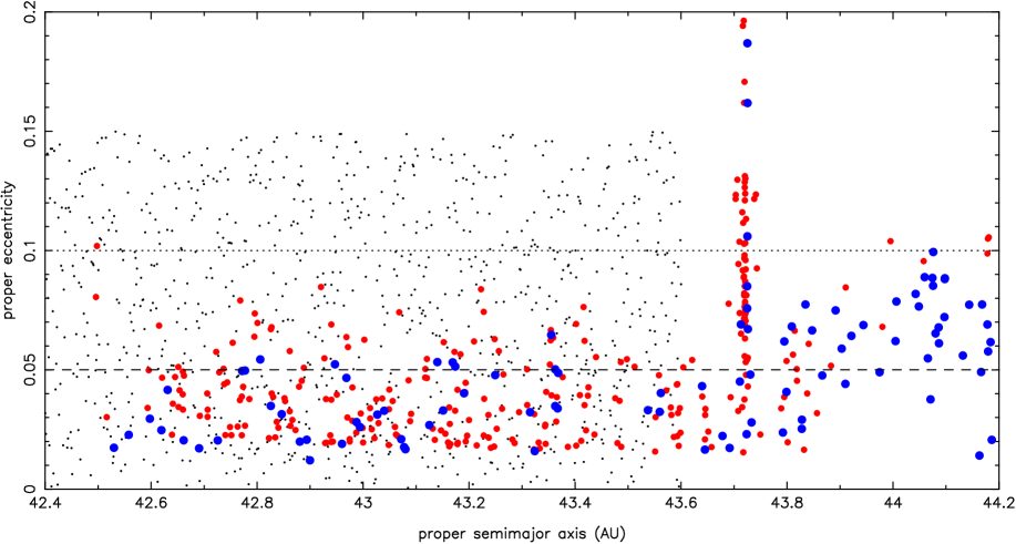
Figure 7: The same as Fig. 3 but for the simulation with initial Neptune’s eccentricity $e_{0}=0.05$ (and still $\tau=$100 My). Notice that in this case the particle population initially extends only up to 43.6 AU.

In the time range up to 150 My, the 4/7 resonance has swept the belt up to 43 AU. The inspection of the final distribution of the particles in the simulation with $e_{0}=0.05$ (Fig. 7) shows that the difference with the $e_{0}=0.1$ case is indeed mostly for particles with $a\lesssim 43$ AU. Specifically, the $e_{0}=0.05$ simulations leaves several particles there with $e>0.05$. whereas the $e_{0}=0.1$ simulation removed almost all of them. This difference is enough to reduce drastically the probability to fit the observed distribution, as reported in Table 1.

This explanation of the importance of the eccentricity of Neptune for the sculpting of the cold population has an interesting implication. It argues that the (already excellent) fit to observations obtained in the simulation with $\tau=100$ My and $e_{0}=0.01$ could improve if the eccentricity of Neptune were damped more slowly than we originally assumed. In fact, the number of particles surviving with $e>0.05$ and $a$ in the 43.0–43.5 AU range would presumably be reduced if Neptune’s eccentricity remained somewhat larger until the 4/7 resonance reached 43.5 AU.

5 Conclusions and discussion

The origin of the cold population of the Kuiper belt is still elusive. A debate is open on whether this population formed in-situ or was transported into the Kuiper belt from a location closer to the Sun during the primordial “wild” evolution of the giant planet orbits.

Dawson and Murray-Clay (2012) pointed out a property of the cold population that had passed previously unnoticed: the inner part of this population (the one with $a<43.5$ AU) has eccentricities smaller than $\sim 0.05$, despite orbits up to $e\sim 0.1$ could be stable in this region. They interpreted this as an evidence that the cold population was only moderately excited from its original circular orbits, which argues in favor of its in-situ formation.

In this work we have confirmed the analysis of Dawson and Murray Clay using proper elements. However, we showed that a slow migration of Neptune (on a timescale of 100 My), initially on a moderately eccentric orbit ($e\sim 0.075$), can reproduce the observations starting from a population uniformly distributed in eccentricity.

Therefore, we disagree that the eccentricity distribution of the inner cold belt can be used as an argument for minor excitation and in-situ formation. Obviously, however, our results do not imply that the cold population formed elsewhere and was transported into the Kuiper belt. It’s origin, therefore, remains elusive.

On this subject, notice from Fig. 1 that the proper eccentricity distribution of the cold population beyond the 4/7 resonance extends up to $\sim 0.1$. It would be strange if the outer population had been excited more than the inner population. This suggests that the entire cold population got strongly excited, so to cover the entire stability region (and probably going beyond it), but it was then depleted near the stability border by the last bit of resonance migration. We also notice in Fig. 1 that beyond the 4/7 resonance there is a deficit of low-eccentricity (i.e. proper $e<0.05$) cold objects, known as the “wedge” (Batygin et al., 2011). If this deficit is not due to observational biases, and it can not be explained the sweeping of the 5/9 resonance. Thus, it is an important diagnostic feature for excitation/implantation models of the cold population.

Our mechanism for the depletion of the inner cold population with moderate eccentricities by resonance sweeping requires a migration timescale of $\sim 100$ My. This timescale is reasonable for a tail-end of the planet migration process, and it is typically observed in simulations where Neptune, after a wild phase of evolution due to close encounters with the other planets, settles down in the planetesimal disk (Gomes et al., 2005; Nesvorny and Morbidelli, 2012). The fact that our mechanism requires that the orbit of Neptune had some moderate eccentricity when its semi major axis was at 28.5 AU argues that the planet underwent previously some form of dynamical instability. The reason is that planetesimal-driven migration can only damp, not excite, the planet’s eccentricity and therefore, without an instability phase, the eccentricity of Neptune would have always been small.

In principle, the eccentricity of Neptune at 28.5 AU could be the remnant of a much larger eccentricity acquired when the planet was closer to the Sun and had close encounters with the other planets. Therefore, the results of this paper are not inconsistent with the scenario of Levison et al. (2008) on the origin of the Kuiper belt, provided that the tail-end of Neptune’s migration is slow enough (which was not the case in Levison et al., who adopted $\tau=1$ My throughout their simulation). However, we acknowledge that said scenario seems to be inconsistent with the existence of wide binaries in the cold population (Parker et al., 2012).

More recently, Nesvorny and Morbidelli (2012) explored the possibility that the outer solar system contained initially an extra Neptune-mass planet, which eventually was ejected during the giant planet instability. In the simulations that reproduced the best the current orbits of the planets, Neptune had an evolution much less wild than that considered in Levison et al. (2008). Neptune migrated out quite smoothly and had only a moderate eccentricity excitation when it encountered the lost planet. It will be important to investigate whether this kind of evolution can transport the cold population into the Kuiper belt via the mechanism of Levison and Morbidelli (2003). This transport mechanism would in principle preserve wide binaries, satisfying the constraint discussed in Parker et al. (2012) and would also be consistent with the results of this paper.

6 References

• Batygin, K., Brown, M. E., Fraser, W. C. 2011. Retention of a Primordial Cold Classical Kuiper Belt in an Instability-Driven Model of Solar System Formation. The Astrophysical Journal 738, 13.

• Brown, M. E. 2001. The Inclination Distribution of the Kuiper Belt. The Astronomical Journal 121, 2804-2814.

• Dawson, R. I., Murray-Clay, R. 2012. Neptune’s Wild Days: Constraints from the Eccentricity Distribution of the Classical Kuiper Belt. The Astrophysical Journal 750, 43.

• Duncan, M. J., Levison, H. F., Budd, S. M. 1995. The Dynamical Structure of the Kuiper Belt. The Astronomical Journal 110, 3073.

• Gladman, B., Marsden, B. G., Vanlaerhoven, C. 2008. Nomenclature in the Outer Solar System. The Solar System Beyond Neptune 43-57.

• Gomes, R. S. 2003. The origin of the Kuiper Belt high-inclination population. Icarus 161, 404-418.

• Gomes, R., Levison, H. F., Tsiganis, K., Morbidelli, A. 2005. Origin of the cataclysmic Late Heavy Bombardment period of the terrestrial planets. Nature 435, 466-469.

• Henrard, J. and Henrard, M. 1991. Slow crossing of a stochastic layer. Physica D 54, 135-146.

• Knežević, Z., Milani, A. 2000. Synthetic Proper Elements for Outer Main Belt Asteroids. Celestial Mechanics and Dynamical Astronomy 78, 17-46.

• Kominami, J., Tanaka, H., Ida, S. 2005. Orbital evolution and accretion of protoplanets tidally interacting with a gas disk. I. Effects of interaction with planetesimals and other protoplanets. Icarus 178, 540-552.

• Levison, H. F., Morbidelli, A. 2003. The formation of the Kuiper belt by the outward transport of bodies during Neptune’s migration. Nature 426, 419-421.

• Levison, H. F., Morbidelli, A., Van Laerhoven, C., Gomes, R., Tsiganis, K. 2008. Origin of the structure of the Kuiper belt during a dynamical instability in the orbits of Uranus and Neptune. Icarus 196, 258-273.

• Lykawka, P. S., Mukai, T. 2005a. Long term dynamical evolution and classification of classical TNO_s. Earth Moon and Planets 97, 107-126.

• Lykawka, P. S., Mukai, T. 2005b. Exploring the 7:4 mean motion resonance I: Dynamical evolution of classical transneptunian objects. Planetary and Space Science 53, 1175-1187.

• Malhotra, R. 1995. The Origin of Pluto’s Orbit: Implications for the Solar System Beyond Neptune. The Astronomical Journal 110, 420.

• Morbidelli A. and Henrard, J., 1993. Slow crossing of a stochastic layer. Physica D. 68, 187-200.

• Morbidelli A., 2002. Modern Celestial Mechanics. Taylor and Francis

• Morbidelli, A., Brown, M. E. 2004. The kuiper belt and the primordial evolution of the solar system. Comets II 175-191.

• Nesvorný, D., Morbidelli, A. 2012. Statistical Study of the Early Solar System’s Instability with Four, Five, and Six Giant Planets. The Astronomical Journal 144, 117.

• Parker, A. H., Kavelaars, J. J., Petit, J.-M., Jones, L., Gladman, B., Parker, J. 2011. Characterization of Seven Ultra-wide Trans-Neptunian Binaries. The Astrophysical Journal 743, 1.