Kink-antikink collisions for twin models

Abstract

In this work we consider kink-antikink collisions for some classes of $(1,1)$-dimensional nonlinear models. We are particularly interested to investigate in which aspect the presence of a general kinetic content in the Lagrangian could be revealed in a collision process. We consider a particular class of models known as twin theories, where different models lead to same solutions for the equations of motion and same energy density profile. The theories can be distinguished in the level of linear stability of defect structure. We study a class of k-defect theories depending on a parameter $M$ which is the twin theory of the usual $\phi^{4}$ theory with standard dynamics. For $M\to\infty$ both models are characterized by the same potential. In the regime $1/M^{2}<<1$, we obtain analytically the spectrum of excitations around the kink solution. It is shown that with the increasing on the parameter $1/M^{2}$: i) the gap between the zero-mode and the first-excited mode increases and ii) the tendency of one-bounce collision between kink-antikink increases. We numerically investigate kink-antikink scattering, looking for the influence of the parameter changing for the thickness and number of two-bounce windows, and confronting the results with our analytical findings.

I Introduction

In this work we consider kink-antikink collisions for some classes of $(1,1)$-dimensional nonintegrable models. As one knows, the collision process for integrable systems has an intrinsic simplicity, with the solitary waves passing to each other with at most a phase shift. Despite this simplicity, analytical results for most integrable models is rather nontrivial. As an example, the analysis of kink-kink and kink-antikink scattering for integrable models using perturbative analysis can be found in Refs. scat1 ; scat2 . For more recent results on this subject, see Refs. scat3 ; scat4 ; scat5 . The effect of a phase shift of the collision process for an integrable model can be confronted to the richness of the collision process for nonintegrable models, where most of analysis must be done numerically. As already shown by Anninos et al aom for the $\lambda\phi^{4}$ theory, for sufficiently small initial velocities, the kink and antikink capture one another and a trapped bion state is formed. On the other hand for larger velocities a simple collision occurs, and after the contact, the pair of defects retreats from each other. For intermediate initial velocities, the structure of the collision is fair more complex, with two-bounce windows appearing in an endless sequence between the larger bion region and the one-bounce ones. A self-similar structure is revealed if one zooms the initial approximation velocity close to the interface regions. Indeed, if one refines the initial velocity near to an interface between a two-bounce window and a bion window, one sees the appearance an endless sequence of three-bounce and bion windows. This refinement process continues with higher number of bounces being observed; however, a limit in this process is achieved due to losses by radiation. The higher number of bounces appears jointly with a higher number of internal mode oscillations. The different windows are related by a scaling relation between the window velocity thickness and the number of internal mode oscillations.

The intriguing character of these alternating regions conflicts with the naive expectation that bion states could not be formed for larger initial velocities than that verified for n-bounce collisions. A semi-phenomenological theory that accounts for the presence of two-bounce windows is due to Campbell et al csw . In their work, the two-bounce behavior is described as a two-steps interacting process. In the first interaction the energy is transferred from the translational mode to an internal shape mode oscillation of the kink. In the second one, if the kink and antikink satisfy a resonance criteria csw ; pc , the energy in the vibrational mode is turned to the translational mode, and the pair $K\bar{K}$ is liberated from their mutual attraction. Quantitatively the simple relation must be obeyed csw

$$\omega_{1}T=2n\pi+\delta$$ (1)

where $\omega_{1}$ is the frequency of the internal mode, T is the time interval between the bounces, $n$ is an integer and $\delta$ is the phase shift between the incoming and outgoing kink. In this way, the higher is $\omega_{1}$, the smaller is the time interval between the bounces, which signals that the energy transference from translational to vibrational mode is more difficult to be achieved. The simple one bounce scattering process occurs for the initial kink velocity higher than a critical velocity $v_{c}$. A heuristic expression for the relation between $T$ and $v$ for the two-bounce windows is presented also in bk , namely

$$T\propto\sqrt{v_{c}-v},\,\,\,v<v_{c}.$$ (2)

The former two expressions can be used to understand quantitatively how the windows centers scale with $n$ bk , with the successive windows with even smaller thickness accumulating near $v=v_{c}$.

The escape of the pair kink-antikink from their mutual attraction is verified when the energy of the vibrational mode is less than the kinetic energy of the colliding kinks bk . Usually one can use collective coordinates to obtain the $K\bar{K}$ attractive interaction potential $U_{K\bar{K}}$ as a function of the separation of the pair kink-antikink kudr ; sug . The potential $U_{K\bar{K}}$ can be intuitively understood as the energy of the static field configuration consisting of a kink at $+Z$ and an antikink at $-Z$ cps . On the other hand, if the time duration of internal oscillations is accompanied by a leaking of energy by radiation greater than the kinetic energy of the colliding kinks, a trapped bion $K\bar{K}$ state is formed bk .

The analysis of kink-antikink collisions can be found in the literature for several interesting examples of nonintegrable models. In addition to the already cited $\lambda\phi^{4}$ model aom , one can cite the modified sine Gordon pc and the $\phi^{6}$ model dmrs . Most of nonintegrable models have internal oscillatory modes, responsible for resonant scattering. However, there are exceptions, as the $\phi^{6}$ model where despite the absence of an internal oscillatory mode, resonant scattering was reported dmrs . There, the potential for linear perturbations has a wide central well and the energy can be transferred from the translational mode to an extended meson state residing in this potential dmrs . Indeed, the central well allow several discrete eigenvalues corresponding to meson-soliton bound states lohe . This is contrary to what happens for the more usual models $\phi^{4}$ and sine-Gordon where mesons can pass through the kink and antikink without reflection, with only a phase shift lohe . In the $\phi^{6}$ model the two-bounce windows satisfy the same relation given by eq. (1), but with $\omega_{1}$ as the frequency of the lowest collective mode. Some interesting discussions related to this topic can also be seen in Ref. weigel .

Our proposal here is to investigate in which measure the kink-antikink collision processes can be used to distinguish twin models, i.e. a class of topological defects with the same scalar field profiles and energy densities altw . For some recent results on this subject, see br ; bhm ; bllm . We are particularly interested in k-defect theories, in part due to their use for explaining the accelerated expansion of the universe k_cosm . Kink-antikink collision processes are useful for cosmology in theories with one extra dimension tm , as in the ekpyrotic proposal for brane collision ekpy . Also, one can cite theories in the braneworld scenario with generalized dynamics bdglm ; blom . The study of bubble cosmology has now being a subject of renewed interest since it can lead to possible ways to probe string landscape pol . Cosmic bubble collisions in the regime of high nucleation rate can be studied ignoring the expansion and the curvature of the universe haw . Despite the usual approach being lattice simulations in $(3,1)$ dimensions egl , in the special situation of bubbles with $SO(2,1)$ symmetry, a high speed collision of two bubbles is equivalent, depending on the vacuum configuration, to a $(1,1)$ dimensional $K\bar{K}$ collision lim . This shows that the studies of $K\bar{K}$ collision in twin theories can be useful for several cosmological scenarios.

In this work, as a starting point we will focus on $(1,1)$-dimensional scalar field theories in the Minkowski spacetime. Despite the simplicity of the proposal, we will show that our results lead to interesting insights about the influence of the k-dynamics on some characteristics of the collision, namely the presence of two-bounce windows. For this purpose, in the Sect. II we review the main first-order formalism for twin theories. Stability analysis is reviewed in Sect. III. Sect. IV specializes the discussion for the $\phi^{4}$ model and its twin theory. The discrete spectra of fluctuations is obtained for mass parameter $1/M^{2}\ll 1$ and compared with known results for the $\phi^{4}$ theory. It is shown that an increasing of the parameter $1/M^{2}$ increases the gap between the zero- and excited modes. This is confronted with our numerical results, presented in Sect. V. Our main conclusions are presented in Sect. VI.

II Twin theories

We start revising some results of the general formalism of k-defects in $(1,1)$ dimensions bab ; asw ; blmo . Consider a general Lagrangian density given by

$$\mathcal{L}=\mathcal{L}(\phi,X)$$ (3)

with

$$X=\frac{1}{2}\partial_{\mu}\phi\partial^{\mu}\phi.$$ (4)

A remark about notation: in this paper a subscript in $\mathcal{L}$ (and later on, in $W$) means partial derivative with respect to the argument. Then for instance $\mathcal{L}_{X}\equiv\partial\mathcal{L}/\partial X$, $\mathcal{L}_{X\phi}\equiv\partial^{2}\mathcal{L}/(\partial X\partial\phi)$ and so on. Now, the equation of motion is given by

$$\partial_{\mu}\left(\mathcal{L}_{X}\partial^{\mu}\phi\right)=\mathcal{L}_{\phi}$$ (5)

or

$$G^{\mu\nu}\partial_{\mu}\partial_{\nu}\phi=-2X\mathcal{L}_{X\phi}+\mathcal{L}_{\phi}$$ (6)

with

$$G^{\mu\nu}=\mathcal{L}_{X}\eta^{\mu\nu}+\mathcal{L}_{XX}\partial^{\mu}\phi\partial^{\nu}\phi$$ (7)

The energy-momentum tensor is

$$T^{\mu\nu}=\mathcal{L}_{X}\partial^{\mu}\phi\partial^{\nu}\phi-\eta^{\mu\nu}\mathcal{L}$$ (8)

and the corresponding energy is

$$E=\int^{\infty}_{-\infty}T^{00}\,dx.$$ (9)

For static solutions, $\phi=\phi(x)$, and Eqs. (6) can be rewritten as

$$\mathcal{L}_{X}A^{2}\phi^{\prime\prime}=-2X\mathcal{L}_{X\phi}+\mathcal{L}_{\phi}$$ (10)

with

$$A^{2}=\frac{2X\mathcal{L}_{XX}+\mathcal{L}_{X}}{\mathcal{L}_{X}}.$$ (11)

Here we will be interested in the corresponding model in the modified k-defect theory of a scalar field model with the standard Lagrangian density

$$\mathcal{L}_{(S)}=X-V(\phi)$$ (12)

where $V(\phi)$ is the potential for the standard theory. The equation of motion for static solutions gives

$$\phi^{\prime\prime}=V_{\phi}$$ (13)

and the energy density is

$$T^{00}\equiv\rho_{S}(x)=\frac{1}{2}{\phi^{\prime}}^{2}+V(\phi).$$ (14)

A very interesting proposal for a corresponding k-defect theory can be found in altw :

$$\mathcal{L}_{(m)}=M^{2}-M^{2}\biggl{(}1+\frac{U(\phi)}{M^{2}}\biggr{)}\sqrt{1-\frac{2X}{M^{2}}}.$$ (15)

where $M$ is a mass scale. As pointed out in bdglm , the limit $1/M^{2}\to 0$ turns this Lagrangian in a standard form with potential $U(\phi)$. In this way we can say $U(\phi)$ is the potential of the modified model. Stable static kinklike solutions must be pressureless ($T^{11}=0$) bdglm ; blmo . In this way the equation of motion gives

$${\phi^{\prime}}^{2}=2U(\phi)+\frac{U^{2}(\phi)}{M^{2}}$$ (16)

and the energy density is

$$\rho_{m}(x)={\phi^{\prime}}^{2}.$$ (17)

If the potentials for the standard and k-defect theory are related by altw

$$V(\phi)=U(\phi)+\frac{1}{2}\frac{U(\phi)^{2}}{M^{2}}$$ (18)

then the models of Eqs. (12) and (15) have the same stable defect structure $\phi(x)$ and energy density altw ; bdglm .

The first-order formalism for general Lagrangian density $\mathcal{L}(X,\phi)$ blm is very useful to understand the connections between the potentials. Introducing a function $W(\phi)$ for the standard Lagrangian density, and for the potential

$$V(\phi)=\frac{1}{2}W_{\phi}^{2}$$ (19)

the solutions of the second-order equation of motion are also solutions of

$$\phi^{\prime}=W_{\phi}.$$ (20)

When applied to the k-defect theory, the corresponding potential is bdglm

$$U(\phi)=-M^{2}+M^{2}\sqrt{1+\frac{W_{\phi}^{2}}{M^{2}}}$$ (21)

III Stability analysis

Here we will review the linear stability of the solutions. We consider $\phi=\bar{\phi}+\eta$, where $\bar{\phi}$ is the unperturbed solution and we suppose small perturbations $\eta$ around this solution. We can use Eq. (6) to attain the first-order contribution in $\eta$

$$\partial_{\mu}\!\!\left(\mathcal{L}_{X}\partial^{\mu}\eta+\mathcal{L}_{XX}\partial^{\mu}\phi\partial_{\alpha}\phi\partial^{\alpha}\eta\right)\!=\!\left[\mathcal{L}_{\phi\phi}\!-\!\partial_{\mu}\!\left(\mathcal{L}_{\phi X}\partial^{\mu}\phi\right)\right]\eta$$ (22)

We decompose the perturbations in terms of the modes

$$\eta(x,t)=\sum_{n}a_{n}\cos(\omega_{n}\,t)\eta_{n}(x)$$ (23)

where the $a_{n}$ are real coefficients. Eq. (23) allow us to rewrite Eq. (22) as blmo

$$-\left[A^{2}\mathcal{L}_{X}\eta_{n}^{\prime}\right]^{\prime}=[\mathcal{L}_{\phi\phi}+(\mathcal{L}_{\phi X}\phi^{\prime})^{\prime}+\omega_{n}^{2}\mathcal{L}_{X}]\eta_{n},$$ (24)

and $A$ was defined in Eq. (11). This is a Sturm-Liouville equation, which means that the eigenfunctions $\eta_{n}$ satisfy a condition of orthonormality with weight function $\mathcal{L}_{X}$ blmo :

$$\int_{-\infty}^{\infty}dx\,\mathcal{L}_{X}\,\eta_{n}(x)\eta_{m}(x)dx=\delta_{mn},$$ (25)

where the eigenfunctions $\eta_{n}$ obey appropriated boundary conditions or $\mathcal{L}_{X}\,$ converges to zero more rapidly than $\,\eta_{n}\left(x\right)$ at boundaries. The finiteness of Eq. (25) must be analyzed in detail for every model to be studied.

The eigenvalue problem (24) becomes more clear after a convenient change of variables (a procedure described in Ref. blm )

$$dx=Adz,~{}~{}\eta_{n}=\frac{u_{n}}{\sqrt{\mathcal{L}_{X}A}},$$ (26)

a Schrödinger-like equation can be obtained

$$-\left(u_{n}\right)_{zz}+U_{sch}(z)u_{n}=\omega_{n}^{2}u_{n},$$ (27)

with blmo

$$U_{sch}(z)=\frac{({A\mathcal{L}_{X}})_{zz}^{\frac{1}{2}}}{({A\mathcal{L}_{X}})^{\frac{1}{2}}}-\frac{1}{{\mathcal{L}}_{X}}\biggl{[}\mathcal{L}_{\phi\phi}+\frac{1}{A}\biggl{(}\mathcal{L}_{\phi X}\frac{\phi_{z}}{A}\biggr{)}_{z}\biggr{]}.$$ (28)

Note that Eq. (27) is an eigenvalue equation where stable solutions correspond to $\omega_{n}^{2}\geq 0$. The existence or not of tachyonic modes ($\omega_{n}^{2}<0$) depends on the model and must be analyzed separately for each case. The determination of the eigenvalues $\omega_{n}$  and stability analysis for the particular case of the $\phi^{4}$ model and its twin counterpart is considered in the next section.

IV The $\phi^{4}$ model and its twin counterpart

In this section we will consider comparatively some properties of two specific twin models. The set of bound states obtained from the stability analysis will give informations that will be confronted later with the numerical analysis of the collisions. It is important to note that, for the models considered in this work, the absence of tachyonic modes is demonstrated in Sect. II of Ref. bdglm . Also, numerical analysis discussing their eigenmodes can be found in two different ways in Refs. altw ; bdglm .

We start considering a standard Lagrangian density with a $\phi^{4}$ potential, where

$$W_{\phi}=1-\phi^{2}.$$ (29)

The kink-like solution of the first-order equation of motion (Eq. (20)) is

$$\phi_{S}(x)=\tanh(x-x_{0})$$ (30)

where $x_{0}$ is a constant, identified as the center of the kink. Note that, as a consequence of the twin model construction, the former expression also corresponds to the solution $\phi_{m}(x)$ achieved for the modified k-defect theory. The first step in the investigation the kink-antikink collision process is to investigate the spectra of fluctuations for both models. The fluctuation modes around the kink are described as $\phi(x,t)=\phi_{S}(x)+\sum_{n}a_{n}\eta_{n}(x)\cos(\omega_{n}t)$. For the standard Lagrangian, a Schrödinger-like equation is attained

$$-\eta_{n}^{\prime\prime}(x)+V_{q}(x)\eta_{n}(x)=\omega_{n}^{2}\eta(x)$$ (31)

with the potential

$$V_{q}(x)=W_{\phi\phi}^{2}+W_{\phi}W_{\phi\phi\phi}=2\big{(}3\tanh^{2}(x)-1\big{)}.$$ (32)

For the twin k-defect model, a Schrödinger-like equation

$$-u_{zz}+U_{q}(z)u=\omega^{2}u,$$ (33)

is possible after a change of variables blm :

$$dx=\biggl{(}1+\frac{W_{\phi}^{2}}{M^{2}}\biggr{)}^{-\frac{1}{2}}dz,$$ (34)

$$\eta=\biggl{(}1+\frac{W_{\phi}^{2}}{M^{2}}\biggr{)}^{\frac{1}{4}}u.$$ (35)

Analytic expressions for the potential $U_{q}(z)$ can be attained in the regime $1/M^{2}\ll 1$. For the particular case $W_{\phi}=1-\phi^{2}$ considered, one gets bdglm

$$U_{q}(z)=4-6\mathrm{sech}^{2}(z)+\frac{1}{M^{2}}[4\mathrm{sech}^{2}(z)+14\mathrm{sech}^{4}(z)-21\mathrm{sech}^{6}(z)].$$ (36)

We see that for $1/M^{2}\to 0$ we have identical potentials $V_{(q)}(z)=U_{(q)}(z)$ for the standard and k-defect theories, with the Schrödinger-like potential being a modified Pösh-Teller. This potential, analyzed in Sugyama sug in the context of $K\bar{K}$ collisions, has two discrete eigenvalues $\omega_{i}^{2}$ with corresponding eingenfunctions $u_{i}(z)$:

$$\omega_{0}^{2}=0,\,\,\,u_{0}(z)=\sqrt{\frac{3}{4}}\mathrm{sech}(z)^{2}$$ (37)

and

$$\omega_{1}^{2}=3,\,\,\,u_{1}(z)=\sqrt{\frac{3}{2}}\tanh(z)\mathrm{sech}(z),$$ (38)

followed by a continuum of modes. The first excited state is an excitation trapped in the kink, crucial for the formation of two-bounce states sug .

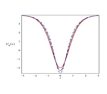
Figure 1: Schrodinger-like potential $U_{q}(z)$ for $1/M^{2}\to 0$ (red line), $0.1$ (black traced line) and $0.2$ (blue point-traced line).

Now, from Fig. 1 we see that the increasing of $1/M^{2}$ leads to the potentials $V_{q}(z)$ and $U_{q}(z)$ to depart one from another, with the Schrödinger-like potential in the k-defect theory with a deeper and thinner potential. Nondegenerate perturbation theory at first-order in the parameter $1/M^{2}\ll 1$ can be used to attain the energy eigenvalues and eigenfunctions of the twin k-defect theory. Eq. (36) can be written as $U_{q}(z)=V_{q}(z)+U_{pert}(z)/M^{2}$, where the perturbation potential is

$$U_{pert}=4\mathrm{sech}^{2}(z)+14\mathrm{sech}^{4}(z)-21\mathrm{sech}^{6}(z).$$ (39)

The ground state energy is invariant under such perturbation:

$$(\omega^{(1)}_{0})^{2} = \omega_{0}^{2}+\frac{1}{M^{2}}\int_{-\infty}^{\infty}dz|u_{0}(z)|^{2}U_{pert}(z)=0.$$ (40)

This means the presence of the translation mode for the corresponding twin model. The energy of the first-excited mode is changed to

$$(\omega^{(1)}_{1})^{2} = \omega_{1}^{2}+\frac{1}{M^{2}}\int_{-\infty}^{\infty}dz|u_{1}(z)|^{2}U_{pert}(z)=3+\frac{8}{5}\frac{1}{M^{2}}.$$ (41)

$1/M^{2}$	$(\omega^{(1)}_{1})^{2}$	$(\omega^{(1)}_{1})_{num}^{2}$	relative error
0	3	3.0000013	$-4.3\times 10^{-7}$
0.01	3.016	3.0159773	$7.5\times 10^{-6}$
0.1	3.16	3.1574820	$8.0\times 10^{-4}$

Table 1: Energy of the first-excited state. In the second column we compare $(\omega^{(1)}_{1})^{2}$, given by Eq. (41) obtained with time-independent perturbed theory. The third column shows the energy obtained numerically with a finite-element method. The fourth column shows the relative error between the results from second and third columns.

Table I shows, for some values of $1/M^{2}$, the evaluated eigenvalue of the internal mode from Eq. (41) and the corresponding numerical solution of the Schröedinger-like equation. We see from the Table that the relative error increases with $1/M^{2}$, with an acceptable value $\sim 10^{-5}$ for $1/M^{2}=0.01$. An increasing of $1/M^{2}$ by one order of magnitude increases the relative error $100$ times. Then, $1/M^{2}=0.1$ seems to be a too large value for the approximation to be valid. Also, from Eqs. (40) and (41), we see that there is a larger gap between the zero-mode and the first excited state with the increasing of the parameter $1/M^{2}$. This property is very important for the whole collision process, since it is in the core of the collision that occurs a transference of energy from translational mode to the vibrational one. If the gap increases, it turns more difficult the energy exchange between the two modes, meaning a disfavoring of the occurrence of bion states and n-bounce collisions with $n\geq 2$ and the enlargement of the range of velocities with one-bounce collisions.

V Numerical Results

Here we will describe our main results concerning to the number of bounces as a function of the initial kink velocity in a symmetric kink-antikink collision. We will consider the standard $\phi^{4}$ theory and twin theories with increasing parameters $1/M^{2}$. Our results will be confronted with the theoretical predictions attained previously in this paper.

V.1 $\lambda\phi^{4}$ theory

First of all we review the $\lambda\phi^{4}$ theory. The equation of motion is

$$\ddot{\phi}-\phi^{\prime\prime}+V_{\phi}=0$$ (42)

where the dots and primes mean derivatives with respect to $t$ and $x$, respectively. We studied a symmetric $K\bar{K}$ collision, with an initial configuration where the pair $K\bar{K}$ is sufficiently separated for the free solution to be useful as an initial condition (kink with velocity $v_{in}$, antikink with velocity $-v_{in}$). This means to chose as the initial conditions

$$\phi(x,0) = \phi_{K}(x+x_{0},v_{in},0)-\phi_{K}(x-x_{0},-v_{in},0)-1$$ (43)

$$\dot{\phi}(x,0) = \dot{\phi}_{K}(x+x_{0},v_{in},0)-\dot{\phi}_{K}(x-x_{0},-v_{in},0).$$ (44)

We used a pseudospectral method on a grid with $2048$ nodes and periodic boundary conditions. We fixed $x_{0}=15$ as the initial kink position and we set the grid boundaries at $x_{max}=120$.

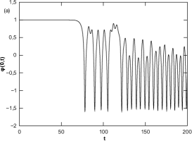
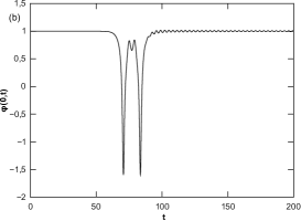
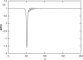
Figure 2: Scalar field $\phi(0,t)$ at the center-of-mass versus t for a) $v_{in}=0.18$ (bion state), b) $v_{in}=0.20$ (two-bounce collision) and c) $v_{in}=0.28$ (one-bounce collision).

For the $\phi^{4}$ model we reproduced some results from the literature aom concerning to the appearance of two-bounce windows. For a particular initial velocity $v_{in}$, the structure of bounces can be easily verified with a plot of the scalar field at the center of mass $\phi(0,t)$ as a function of $t$. Some examples for three different initial velocities can be seen in Figs. 2, where we have a bion (2a), two-bounce (2b) and one-bounce (2c) collisions. As one knows, the dependence of the number of bounces with the modulus of the initial velocity $v_{in}$ of the pair kink-antikink is intricate. For low $v_{in}$ a bion state is formed, whereas for high $v_{in}$ one has a one-bounce scattering. For intermediate velocities, there appears two-bounce windows of variable size separated by regions of bion states.

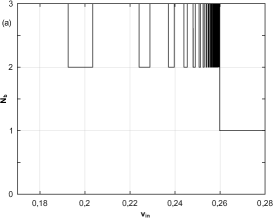
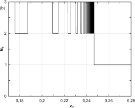
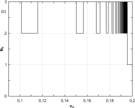
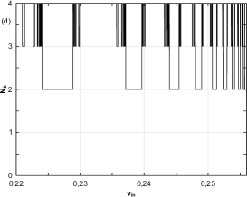
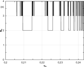
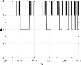
Figure 3: Number of bounces versus initial velocity $v_{in}$, a) for $\phi^{4}$ model (upper left) and b) for twin model with $1/M^{2}=0.01$ (upper center) and $1/M^{2}=0.05$ (upper right), showing the presence of two-bounce windows. After zooming the interval, three-bounce windows can be seen in the corresponding lower figures, for d) $\phi^{4}$ model (lower left) and e) twin model with $1/M^{2}=0.01$ (lower center) and f) twin model with $1/M^{2}=0.05$ (lower right) .

We constructed a procedure to identify the number of bounces $N_{b}$ for a given collision process in a time interval $0<t<T=200s$. We defined a bounce as connected to the change of sign of the center-of-mass solution $\phi(0,t)$. In this way, Fig. 2b and 2c show collisions with $N_{b}=2$ and $N_{b}=1$, respectively and 2a shows a bion state. In our analysis, a too large value of $N_{b}$ will correspond to a bion state. Fig. 3a shows the behavior of $N_{b}$ as a function of $v_{in}$. Note from the figure the change of pattern for collisions around $v_{in}\sim 0.26$. The presence of higher number of bounces for $v_{in}\lesssim 0.26$ characterizes bion states, whereas there are intermediate regions with $N_{b}=2$. States with $N_{b}=1$ appear for $v_{in}\gtrsim 0.26$. The structure of the two-bounce windows can be characterized by the integer $m$ labeling the number of oscillations in $\phi(0,t)$ between the bounces. For example, in the Fig. 3a the first two-bounce window corresponds to $m=1$ (see details in Ref. aom ). The two-bounce thickness decreases with $m$ accumulating around $v_{in}\simeq 0.26$, the limit above which the initial velocity is already sufficiently large for a one-bounce scattering. Table II shows some characteristics of the thickness of the first four two-bounce windows. This table shows how an increasing in $m$ reflects in the reducing of the two-bounce windows. This can be better seen in Fig. 4 (see Ref. bk ).

m	$v_{1}$	$v_{2}$	$\Delta v$	$v_{1T}$	$v_{2T}$	$\Delta{v_{T}}$
1	0.1926	0.2034	0.0108	0.1757	0.1872	0.0115
2	0.2241	0.2288	0.0047	0.2095	0.2145	0.005
3	0.2372	0.2396	0.0024	0.2233	0.2259	0.0026
4	0.2440	0.2454	0.0014	0.2305	0.2320	0.0015

Table 2: Separation in velocities of the first four two-bounce windows. $m$ is a label corresponding to the particular two-bounce window (equal to the number of oscillations of $\phi(0,t)$ between the two bounces). For the $\phi^{4}$ model, the columns $v_{1}$ and $v_{2}$ correspond to the first and last points of the velocity of the window and $\Delta v$ the corresponding width (the numerical results are in agreement with Table II of cp ). For the twin k-defect model with $1/M^{2}=0.01$, columns to the right show similar informations identified by $v_{1T}$, $v_{2T}$ and $\Delta v_{T}$.

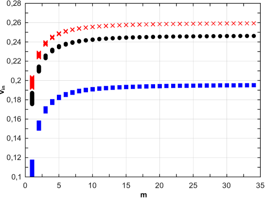
Figure 4: Intervals in velocities inside which the pair kink-antikink escape after a two-bounce collision as a function of $m$, the number of small oscillations of $\phi(0,t)$ near vacuum between the two-bounces a) for $\phi^{4}$ model (red crosses), b) for twin model with $1/M^{2}=0.01$ (black circles) and c) for twin model with $1/M^{2}=0.05$ (blue squares).

Also refining the input data of initial velocities around a border between a two-bounce window and bion, one sees the presence of a cascate of three-bounce windows, as can be seen in Fig. 3d. Note that the three-bounce windows accumulate around the border of the two-bounce windows, replicating the effect of reducing of thickness and separation of windows that occurs in Fig. 3a, and showing the well-known fractal pattern of $K\bar{K}$ collisions for the $\phi^{4}$ model.

V.2 twin theory

The twin theory in the regime $1/M^{2}\ll 1$ has the corresponding equation of motion

$$\ddot{\phi}-\phi^{\prime\prime}+\frac{1}{M^{2}}(\dot{\phi}^{2}\ddot{\phi}+\phi^{\prime 2}\phi^{\prime\prime}-2\dot{\phi}\phi^{\prime}\dot{\phi}^{\prime})+U_{\phi}-\frac{1}{M^{2}}UU_{\phi}=0.$$ (45)

In the regime $1/M^{2}\ll 1$, and neglecting terms of ${\mathcal{O}}(1/M^{4})$ we have

$$U(\phi)=\frac{1}{2}W_{\phi}^{2}-\frac{1}{8}\frac{W_{\phi}^{4}}{M^{2}}.$$ (46)

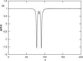
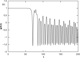
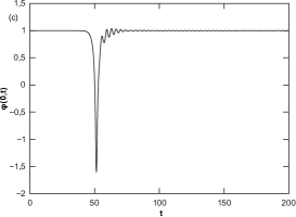
Figure 5: Scalar field $\phi(0,t)$ at the center-of-mass versus t for a) $v_{in}=0.18$ (two-bounce collision), b)$v_{in}=0.20$ (bion state) and c) $v_{in}=0.28$ (one-bounce collision) for twin model with $1/M^{2}=0.01$.

Substituting this in Eq. (45), one can easily verify that $\phi_{K}(x,t)=\tanh(\gamma(x-vt))$ is the solution for a free propagating kink. As expected this is the same solution already achieved for the $\phi^{4}$ model. This means that the initial conditions will be the same used for the $\phi^{4}$ model. Indeed, it is only the collision process that will distinguish both theories. Also, as used previously for the $\phi^{4}$ theory, this analytic solution can be used as a first test for the numerical solution for the twin theories. In Figs. 5 we present some results for $\phi(0,t)$ for the twin theory with $1/M^{2}=0.01$. Comparing the figures with Fig. 2 for the $\phi^{4}$ theory we see that even for a small value of $1/M^{2}$ the behavior is altered sensibly. For example, for $v_{in}=0.2$ we have two-bounce collision with $m=1$ for the $\phi^{4}$ model (Fig. 2b) and bion for the twin model (Fig. 5b). Also, for $v_{in}=0.18$ we have bion for the $\phi^{4}$ model (Fig. 2a) and two-bounce collision with $m=1$ for the twin model (Fig. 5a). Our results of $N_{b}$ as a function of $v_{in}$ for $1/M^{2}=0.01$ are depicted in Fig. 3b. The same effect of appearance of two-bounce windows already known for the $\phi^{4}$ model is present for the twin model. In the twin model, however, the one-bounce collision occurs for $v_{in}\gtrsim 0.246$, smaller that $v_{in}\gtrsim 0.26$ for the $\phi^{4}$ theory. An increasing of $1/M^{2}$ shows the same pattern, as can be seen in Fig. 3c for $1/M^{2}=0.05$, where now the one-bounce collisions occur for $v_{in}\simeq 0.20$. This enlargement of the region where occurs the one-bounce window is directly related to the increasing of the gap between the translational and vibrational modes, as discussed in the final of the previous section.

Table II shows the separation in velocities of the first four two-bounce windows for both $\phi^{4}$ and the twin model for $1/M^{2}=0.01$. We see that the thickness of the windows are roughly the same, occurring for lower velocities in the twin model in comparison to the $\phi^{4}$ model. This can be better seen in Fig. 4, where we also included the case where $1/M^{2}=0.05$. There one can also see that, similarly to the $\phi^{4}$ model, for the twin model the velocity thickness is reduced continuously with $m$, whereas $v_{in}$ grows and asymptotes to the minimum velocity $v_{in}^{*}$ for the occurrence of a one-bounce collision. Also note from the figure that the larger is $1/M^{2}$, the lower is $v_{in}^{*}$.

For the twin model we refined the input data of initial velocities around a border between a two-bounce window and bion, obtaining the results of Figs. 3e and 3f. There one can see the presence of a cascate of three-bounce windows, accumulating around the border of the two-bounce windows, replicates the effect of reducing of thickness and separation of windows that occurs in the corresponding Figs. 3b and 3c, and showing that there is a fractal pattern of $K\bar{K}$ collisions for the twin model in a similar way to the verified for $\phi^{4}$ model (compare with Figs. 3a and 3d).

Fig. 6a-b show the time $t$ of the first three bounces as a function of the initial velocity $v_{in}$. Our results with $1/M^{2}=0.01$ (Fig. 6b) clearly show that there is a displacement of the two-bounce windows for regions of lower velocities in comparison to the $\phi^{4}$ model (compare with Fig. 6a). This can be interpreted as a signal of a weaker $K\bar{K}$ interaction for the twin model, in comparison to the $\phi^{4}$ model.

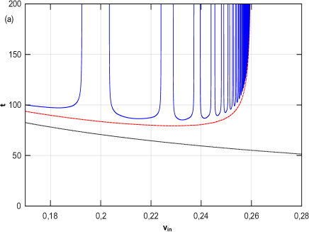
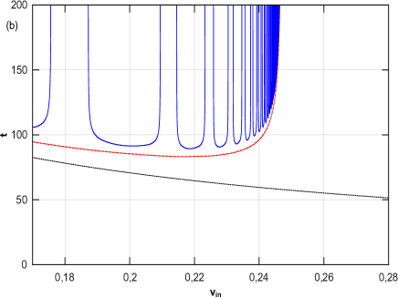
Figure 6: Times to the first (black line), second (red long trace) and third (blue short trace) bounces in a $K\bar{K}$ collision, as a function of the initial velocity, for a) $\phi^{4}$ model and b) twin model with $1/M^{2}=0.01$.

We also investigated if the fundamental relation given by Eq. (1) holds in the modified twin model. In Fig. 7 we plot the time between bounces versus $n=m+2$, where $m$ is the window number. The integer $n$ is constructed in order to achieve a phase shift $\delta$ between $0$ and $2\pi$. We note from the figure that the numerical points can be described with good approximation by a straight line. Table III compares the angular coefficients from the least-squares with the theoretical one $2\pi/\omega_{1}$, predicted by Eq. (1). From the Table we see that for $1/M^{2}=0$ the theoretical angular coefficient $2\pi/(\omega^{(1)}_{1})$ is lower but comparable to the numerical value obtained by least-squares method, as already noted in Ref. aom . Also Table III shows that the numerical angular coefficient grows with the increasing of $1/M^{2}$. This is an intriguing character, since from Eq. (1) it is expected a decreasing of the angular coefficient, as shown in the second row of Table III. Since we found no physical ground for such behavior, we must say this numerical result must be handled with care, for the following reasons: i) One must note that Fig. 7 considers a quite large number of windows (up to $m\sim 35$). As the window number grows, also grows the numerical error of the simulations. To put in other words, a consistent numerical analysis of two-bounce windows is easier from the computational perspective. ii) Eq. (1) was proposed by Campbell et all in Ref. as a good simplification of an intrincate process of interaction between two extended objects. If we want to test a qualitative expression, we must not be so strict in quantitative agreement. iii) We cannot consider a too large value of $1/M^{2}$ as a valid approximation of a twin theory breaks. We could take $1/M^{2}=0.05$ as a higher bound for an analysis of a two-bounce windows, but this value could be even lower for larger number of bounces. In this paper, all the former numerical results and analysis concerning to two-bounce windows where shown to be compatible with the interpretation of Eq. (1). The aplicability of this equation can be confirmed also by Fig. 7 and Table III in the sense that a straight line behavior was verified and the angular coefficients are roughly comparable, as already done in Ref. aom for the $\phi^{4}$ model.

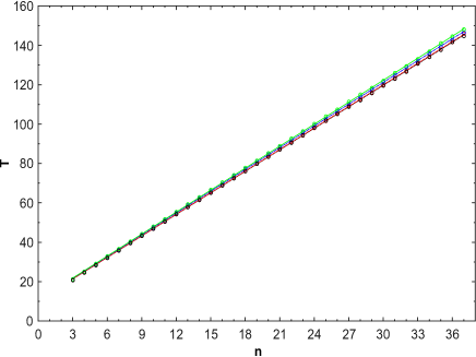
Figure 7: Time between bounces versus $n=m+2$, where $m$ is the window number for a) $1/M^{2}=0$ (dotted black), b) $1/M^{2}=0.01$ (traced red), c) $1/M^{2}=0.05$ (dot-traced blue) and d) $1/M^{2}=0.08$ (solid green). For fixed $1/M^{2}$ circles represents numerical results, whereas line is a least-square fitting.

$1/M^{2}$	$2\pi/(\omega^{(1)}_{1})$	$a$	relative error
0	3.63	3.65	$0.55\%$
0.01	3.62	3.66	$1.1\%$
0.05	3.58	3.69	$3.0\%$

Table 3: Theoretical angular coefficient $2\pi/(\omega^{(1)}_{1})$ versus angular coefficient $a$ obtained by least-squares method from Fig. 7.

VI conclusions

In this work we have studied kink-antikink collisions for twin theories. We were particularly interested in investigating in which aspect the presence of a general kinetic content (k-generalization) in the Lagrangian could be revealed in a collision process. Starting form a general Lagrangian $\mathcal{L}(X,\phi)$, and considering a convenient decomposition of the fluctuations, we analyzed the energy contribution of the fluctuations. After reviewing the first-order formalism of twin theories, we considered the $\phi^{4}$ theory and a class of twin theories depending on a mass parameter $M$. In the regime where $1/M^{2}\ll 1$, we obtained the spectra of excitations with two bound states: a zero-mode, responsible for the translation, and a vibrational one, crucial for the two-bounce collisions. We showed that the gap between the two bound states is larger for the twin model, and that it increases with $1/M^{2}$. A detailed numerical analysis reproduced some known results for $K\bar{K}$ collisions in the $\phi^{4}$ theory, used as a control model to be confronted with the results of a twin model of a general kinetic content. The numerical results corroborated the theoretical expectation that, in a collision process, the increasing of $1/M^{2}$ reduces the possibility of formation of a trapped $K\bar{K}$ bion state.

VII Acknowledgements

The authors thank FAPEMA, CAPES, CNPq and IFMA for financial support. The authors thank Herbert Weigel and R. Casana for clarifying several points of stability analysis. A. R. Gomes thanks A. S. Anjos and M. M. Ferreira Jr. for discussions.

References

- (1) B. A. Malomed, Physica D: Nonlinear Phenomena 15, 385 (1985).
- (2) D. W. McLaughlin and A. C. Scott, Phys. Rev. A 18, 1652 (1978).
- (3) M. A. Amin, Phys. Rev. D87, 123505 (2013)
- (4) M. A. Amin, E. A. Lim, I. Sheng Yang, Phys.Rev.Lett. 111 (2013) 224101
- (5) M. A. Amin, E. A. Lim, I. Sheng Yang, Phys.Rev. D88 (2013) 105024.
- (6) P. Anninos, S. Oliveira, R. A. Matzner, Phys. Rev. D 44, 1147 (1991).
- (7) D. K. Campbell, J. F. Shonfeld, C. A. Wingate, Physica D 9, 1 (1983).
- (8) M. Peyrard, D.K. Campbell, Physica D 9, 33 (1983).
- (9) T. Belova and A. Kudryavtsev, Physica D 32, 18 (1988).
- (10) A.E. Kudryavtsev, JETP Lett. 22, 82 (1975).
- (11) T. Sugiyama, Prog. Theor. Phys. 61, 1550 (1979).
- (12) D. K. Campbell, M. Peyrard, P. Sodano, Physics D 19, 165 (1986).
- (13) P. Dorey, K. Mersh, T. Romanczukiewicz, Y. Shnir, Phys.Rev.Lett. 107, 091602 (2011).
- (14) M. A. Lohe, Phys. Rev. D 20, 3120 (1979).
- (15) H. Weigel, J. Phys. Conf. Series, 482 (2014) 012045.
- (16) M. Andrews, M. Lewandowski, M. Trodden, and D. Wesley, Phys. Rev. D 82, 105006 (2010).
- (17) D. Bazeia, R. Menezes, Phys.Rev. D 84, 125018 (2011).
- (18) D. Bazeia, E. da Hora, R. Menezes, Phys.Rev. D85, 045005 (2012).
- (19) D. Bazeia, A.S. Lobão, L. Losano, R. Menezes, Eur. Phys. J. C74 (2014) 2755.
- (20) C. Armendariz-Picon, T. Damour, and V. F. Mukhanov, Phys. Lett. B 458, 209 (1999); J. Garriga and V. F. Mukhanov, Phys. Lett. B 458, 219 (1999); T. Chiba, T. Okabe, and M. Yamaguchi, Phys. Rev. D 62, 023511 (2000).
- (21) Y. I. Takamizu and K. I. Maeda, Phys. Rev. D 70, 123514 (2004); ibid Phys. Rev. D 73, 103508 (2006).
- (22) J. Khoury, B.A. Ovrut, P. J. Steinhardt, and N. Turok, Phys. Rev. D 64, 123522 (2001); J. Khoury, B.A. Ovrut, N. Seiberg, P. J. Steinhardt, and N. Turok, ibid. 65, 086007 (2002); J. Khoury, B.A. Ovrut, P. J. Steinhardt, and N. Turok, ibid. 66, 046005 (2002); A. J. Tolley and N. Turok, ibid. 66, 106005 (2002).
- (23) D. Bazeia, J. D. Dantas, A. R. Gomes, L. Losano and R. Menezes, Phys.Rev. D84, 045010 (2011).
- (24) D. Bazeia, A.S. Lobao, Jr., R. Menezes, Phys.Rev. D 86, 125021 (2012).
- (25) R. Bousso and J. Polchinski, J. High Energy Phys. 06, 006 (2000).
- (26) S. W. Hawking, I. G. Moss, J. M. Stewart, Phys. Rev. D 26, 2681 (1982).
- (27) R. Easther, J. T. Giblin Jr., Lam Hui, E. A. Lim, Phys. Rev. D 80, 123519 (2009).
- (28) J. T. Giblin Jr., Lam Hui, E. A. Lim, I. Sheng Yang, Phys. Rev. D 82, 045019 (2010).
- (29) E. Babichev, Phys. Rev. D 74, 085004 (2006).
- (30) C. Adam, J. Sanchez-Guillen, A. Wereszczynski, J. Phys. A 40, 13625 (2007).
- (31) D. Bazeia, L. Losano, R. Menezes and J. C. R. E. Oliveira, Eur. Phys. J. C 51, 953 (2007).
- (32) D. Bazeia, L. Losano and R. Menezes, Phys. Lett. B 668, 246 (2008).
- (33) D.K. Campbell, M. Peyrard, Physica D 18, 47 (1986).