Zhongkui Li, Zhisheng Duan, Wei Ren, Gang Feng

Abstract: This paper considers the containment control problem for multi-agent systems with general linear dynamics and multiple leaders whose control inputs are possibly nonzero and time varying. Based on the relative states of neighboring agents, a distributed static continuous controller is designed, under which the containment error is uniformly ultimately bounded and the upper bound of the containment error can be made arbitrarily small, if the subgraph associated with the followers is undirected and for each follower there exists at least one leader that has a directed path to that follower. It is noted that the design of the static controller requires the knowledge of the eigenvalues of the Laplacian matrix and the upper bounds of the leaders’ control inputs. In order to remove these requirements, a distributed adaptive continuous controller is further proposed, which can be designed and implemented by each follower in a fully distributed fashion. Extensions to the case where only local output information is available are discussed.

Keywords: Multi-agent systems, containment control, cooperative control, consensus, adaptive control.

1 Introduction

Consensus is a fundamental problem in the area of cooperative control of multi-agent systems and has attracted a lot of interest from the systems and control community in the last decade. Consensus means that a group of agents reaches an agreement on a physical quantity of interest by interacting with their local neighbors. For recent advances of the consensus problem, readers are referred to [1, 2, 3, 4, 5, 6, 7, 8, 9, 10, 11] and references therein. Roughly speaking, existing consensus algorithms can be categorized into two classes, namely, consensus without a leader and consensus with a leader. The case of consensus with a leader is also called leader-follower consensus or distributed tracking.

The distributed tracking problem deals with only one leader. However, in some practical applications, there might exist more than one leader in agent networks. In the presence of multiple leaders, the containment control problem arises, where the followers are to be driven into a given geometric space spanned by the leaders [12]. The study of containment control has been motivated by many potential applications. For instance, a group of autonomous vehicles (designated as leaders) equipped with necessary sensors to detect the hazardous obstacles can be used to safely maneuver another group of vehicles (designated as followers) from one target to another, by ensuring that the followers are contained within the moving safety area formed by the leaders [12, 13]. A hybrid containment control law is proposed in [12] to drive the followers into the convex hull spanned by the leaders. Distributed containment control problems are studied in [14, 13, 15] for a group of first-order and second-order integrator agents under fixed and switching directed communication topologies. The containment control is considered in [16] for second-order multi-agent systems with random switching topologies. A hybrid model predictive control scheme is proposed in [17] to solve the containment and distributed sensing problems in leader/follower multi-agent systems. The authors in [18, 19, 20] study the containment control problem for a collection of Euler-Lagrange systems. In particular, [19] discusses the case with multiple stationary leaders, [20] studies the case of dynamic leaders with finite-time convergence, and [18] considers the case with parametric uncertainties. In the above-mentioned works, the agent dynamics are assumed to be single, double integrators, or second-order Euler-Lagrange systems, which might be restrictive in some circumstances. The containment control for multi-agent systems with general linear dynamics is considered in [21], which however assumes the leaders’ control inputs to be zero. In many cases, the leaders might need nonzero control actions to regulate their state trajectories, e.g., to avoid obstacles or to form a desirable safety area.

In this paper, we study the distributed containment control problem for multi-agent systems with general linear dynamics and multiple leaders whose control inputs are possibly nonzero and time varying. Based on the relative states of neighboring agents, a distributed discontinuous controller is designed to ensure that the containment error asymptotically converges to zero, if the subgraph associated with the followers is undirected and for each follower there exists at least one leader that has a directed path to that follower. It is pointed out that the discontinuous controller may cause the undesirable chattering phenomenon in real implementation. To eliminate the chattering effect, using the boundary layer concept, a static continuous containment controller is then constructed, under which the containment error is uniformly ultimately bounded and the upper bound of the containment error can be made arbitrarily small. It is noted that the design of this static containment controller requires the knowledge of the eigenvalues of the Laplacian matrix and the upper bounds of the leaders’ control inputs. In order to remove these requirements, a distributed adaptive continuous containment controller is further proposed. A distinct feature of the proposed adaptive containment controller is that it can be designed and implemented by each follower in a fully distributed fashion without requiring any global information. Extensions to the case where only local output information is available are discussed. Based relative estimates of the states of neighboring agents, distributed observer-based containment controllers are proposed. A sufficient condition for the existence of these containment controllers is that each agent is stabilizable and detectable.

Compared to the previous works [12, 14, 13, 15, 16, 18, 19, 20, 21], the contribution of this paper is at least three-fold. First, in contrast to [12, 14, 13, 15, 16, 18, 19, 20] which puts restrictions on the agent dynamics and [21] which assumes the leaders’ control inputs to be zero, the results obtained in this paper are applicable to multi-agent systems with general linear dynamics and multiple leaders whose control inputs are possibly nonzero and bounded. Second, contrary to the discontinuous controllers in [14, 13, 15, 20, 18], a distinct feature of the proposed containment controllers is that they are continuous, for which case the undesirable chattering phenomenon can be avoided. It is worth mentioning that with the discontinuous functions replaced with the continuous ones, it is no longer clear how the controllers and the adaptive gain design will function. It is hence challenging to analyze and show the ultimate boundedness of the containment errors and the adaptive coupling gains using the proposed continuous controllers. Third, the adaptive containment controllers proposed in this paper can be implemented in a fully distributed fashion without requiring any global information.

The rest of this paper is organized as follows. Some useful results of the graph theory and ultimate boundedness are reviewed in Section 2. The containment control problem is formulated and discontinuous containment controllers are proposed in Section 3. Distributed static and adaptive continuous containment controllers based on the relative state information are considered in Section 4. Extensions to the case with output feedback controllers are discussed in Section 5. Simulation examples are presented in Section 6 to illustrate the analytical results. Conclusions are drawn in Section 7.

2 Mathematical Preliminaries

2.1 Notations

Let $\mathbf{R}^{n\times n}$ be the set of $n\times n$ real matrices. The superscript $T$ means transpose for real matrices. $I_{N}$ represents the identity matrix of dimension $N$. Denote by $\mathbf{1}$ a column vector with all entries equal to one. $\mathrm{diag}(A_{1},\cdots,A_{n})$ represents a block-diagonal matrix with matrices $A_{i},i=1,\cdots,n,$ on its diagonal. For real symmetric matrices $X$ and $Y$, $X>(\geq)Y$ means that $X-Y$ is positive (semi-)definite. $A\otimes B$ denotes the Kronecker product of matrices $A$ and $B$. For a vector $x\in\mathbf{R}^{n}$, let $\|x\|$ denote its 2-norm. For a symmetric matrix $A$, $\lambda_{\min}(A)$ and $\lambda_{\max}(A)$ denote, respectively, the minimum and maximum eigenvalues of $A$. A matrix is Hurwitz (stable) if all of its eigenvalues have strictly negative real parts.

2.2 Graph Theory

A directed graph $\mathcal{G}$ is a pair $(\mathcal{V},\mathcal{E})$, where $\mathcal{V}=\{v_{1},\cdots,v_{N}\}$ is a nonempty finite set of nodes and $\mathcal{E}\subseteq\mathcal{V}\times\mathcal{V}$ is a set of edges, in which an edge is represented by an ordered pair of distinct nodes. For an edge $(v_{i},v_{j})$, node $v_{i}$ is called the parent node, node $v_{j}$ the child node, and $v_{i}$ is a neighbor of $v_{j}$. A graph with the property that $(v_{i},v_{j})\in\mathcal{E}$ implies $(v_{j},v_{i})\in\mathcal{E}$ for any $v_{i},v_{j}\in\mathcal{V}$ is said to be undirected. A path from node $v_{i_{1}}$ to node $v_{i_{l}}$ is a sequence of ordered edges of the form $(v_{i_{k}},v_{i_{k+1}})$, $k=1,\cdots,l-1$. A subgraph $\mathcal{G}_{s}=(\mathcal{V}_{s},\mathcal{E}_{s})$ of $\mathcal{G}$ is a graph such that $\mathcal{V}_{s}\subseteq\mathcal{V}$ and $\mathcal{E}_{s}\subseteq\mathcal{E}$. A directed graph contains a directed spanning tree if there exists a node called the root, which has no parent node, such that the node has directed paths to all other nodes in the graph.

The adjacency matrix $\mathcal{A}=[a_{ij}]\in\mathbf{R}^{N\times N}$ associated with the directed graph $\mathcal{G}$ is defined by $a_{ii}=0$, $a_{ij}=1$ if $(v_{j},v_{i})\in\mathcal{E}$ and $a_{ij}=0$ otherwise. The Laplacian matrix $\mathcal{L}=[\mathcal{L}_{ij}]\in\mathbf{R}^{N\times N}$ is defined as $\mathcal{L}_{ii}=\sum_{j\neq i}a_{ij}$ and $\mathcal{L}_{ij}=-a_{ij}$, $i\neq j$. For undirected graphs, both $\mathcal{A}$ and $\mathcal{L}$ are symmetric. It is easy to see that zero is an eigenvalue of $\mathcal{L}$ with $\mathbf{1}$ as a corresponding right eigenvector and all nonzero eigenvalues have positive real parts. Furthermore, zero is a simple eigenvalue of $\mathcal{L}$ if and only if $\mathcal{G}$ has a directed spanning tree [22, 23].

3 Problem Formulation and Discontinuous Containment Controllers

Consider a group of $N$ agents with general continuous-time linear dynamics, described by

$$\dot{x}_{i} =Ax_{i}+Bu_{i},$$ (1)

$$y_{i} =Cx_{i},\quad i=1,\cdots,N,$$

where $x_{i}\in\mathbf{R}^{n}$, $u_{i}\in\mathbf{R}^{p}$, and $y_{i}\in\mathbf{R}^{q}$ are, respectively, the state, the control input, and the output of the $i$-th agent, and $A$, $B$, $C$, are constant matrices with compatible dimensions.

In this paper, we consider the case where there exist multiple leaders. Suppose that there are $M$ ($M<N$) followers and $N-M$ leaders. An agent is called a leader if it has no neighbor and is called a follower if it has at least one neighbor. Without loss of generality, we assume that the agents indexed by $1,\cdots,M$, are followers, while the agents indexed by $M+1,\cdots,N$, are leaders. We use $\mathcal{R}\triangleq\{M+1,\cdots,N\}$ and $\mathcal{F}\triangleq\{1,\cdots,M\}$ to denote, respectively, the leader set and the follower set. The communication graph among the $N$ agents is represented by a directed graph $\mathcal{G}$, which satisfies the following assumption.

Assumption 1. The subgraph $\mathcal{G}_{s}$ associated with the $M$ followers is undirected. For each follower, there exists at least one leader that has a directed path to that follower.

Denote by $\mathcal{L}$ the Laplacian matrix associated with $\mathcal{G}$. Because the leaders have no neighbors, it is easy to see that $\mathcal{L}$ can be partitioned as

$$\mathcal{L}=\begin{bmatrix}\mathcal{L}_{1}&\mathcal{L}_{2}\\ 0_{(N-M)\times M}&0_{(N-M)\times(N-M)}\end{bmatrix},$$ (2)

where $\mathcal{L}_{1}\in\mathbf{R}^{M\times M}$ is symmetric and $\mathcal{L}_{2}\in\mathbf{R}^{M\times(N-M)}$.

Lemma 1 [20]. Under Assumption 1, all the eigenvalues of $\mathcal{L}_{1}$ are positive, each entry of $-\mathcal{L}_{1}^{-1}\mathcal{L}_{2}$ is nonnegative, and each row of $-\mathcal{L}_{1}^{-1}\mathcal{L}_{2}$ has a sum equal to one.

Different from the previous work [21] which assumes the leaders’ control inputs $u_{i}$, $i\in\mathcal{R}$, to be zero, we consider here the general case where the leaders’ control inputs are possibly nonzero and time varying. Suppose that the following mild assumption holds.

Assumption 2. The leaders’ control inputs $u_{i}$, $i\in\mathcal{R}$, are bounded, i.e., $\|u_{i}\|\leq\gamma_{i}$, $i\in\mathcal{R}$, where $\gamma_{i}$ are positive constants.

The objective of this paper is to solve the distributed containment control problem for the agents in (1), i.e., to design distributed controllers under which the states of the $M$ followers can converge to the convex hull spanned by the states of the leaders.

Note that the leaders’ control inputs are generally available to at most a subset of the followers. In order to solve the containment problem, based on the relative state information of neighboring agents, we propose a distributed static controller for each follower as

$$u_{i} =c_{1}K\sum_{j=1}^{N}a_{ij}(x_{i}-x_{j})+c_{2}\hat{g}\left(K\sum_{j=1}^{N}a_{ij}(x_{i}-x_{j})\right),\quad i\in\mathcal{F},$$ (3)

where $c_{1}>0$ and $c_{2}>0\in\mathbf{R}$ are constant coupling gains, $K\in\mathbf{R}^{p\times n}$ is the feedback gain matrix, $a_{ij}$ is the $(i,j)$-th entry of the adjacency matrix $\mathcal{A}$ associated with $\mathcal{G}$, and the nonlinear function $\hat{g}(\cdot)$ is defined as follows: for $w\in\mathbf{R}^{n}$,

$$\hat{g}(w)=\begin{cases}\frac{w}{\|w\|}&\text{if}~{}\|w\|\neq 0,\\ 0&\text{if}~{}\|w\|=0.\end{cases}$$ (4)

Let $x_{f}=[x_{1}^{T},\cdots,x_{M}^{T}]^{T}$, $x_{l}=[x_{M+1}^{T},\cdots,x_{N}^{T}]^{T}$, $x=[x_{f}^{T},x_{l}^{T}]^{T}$, and $u_{l}=[u_{M+1}^{T},\cdots,u_{N}^{T}]^{T}$. Then, it follows from (1) and (3) that the closed-loop network dynamics can be written as

$$\dot{x}_{f} =(I_{M}\otimes A+c_{1}\mathcal{L}_{1}\otimes BK)x_{f}+c_{1}(\mathcal{L}_{2}\otimes BK)x_{l}+c_{2}(I_{M}\otimes B)G(x),$$ (5)

$$\dot{x}_{l} =(I_{N-M}\otimes A)x_{f}+(I_{M}\otimes B)u_{l},$$

where $\mathcal{L}_{1}$ and $\mathcal{L}_{2}$ are defined as in (2), and $\widehat{G}(x)\triangleq\begin{bmatrix}\hat{g}(K\sum_{j=1}^{N}a_{1j}(x_{1}-x_{j}))\\ \vdots\\ \hat{g}(K\sum_{j=1}^{N}a_{Mj}(x_{M}-x_{j}))\end{bmatrix}.$

Introduce the following variable:

$$\xi\triangleq x_{f}+(\mathcal{L}_{1}^{-1}\mathcal{L}_{2}\otimes I_{n})x_{l},$$ (6)

where $\xi=[\xi_{1}^{T},\cdots,\xi_{M}^{T}]^{T}$. From (6), it is easy to see that $\xi=0$ if and only if $x_{f}=(-\mathcal{L}_{1}^{-1}\mathcal{L}_{2}\otimes I_{n})x_{l}$. In virtue of Lemma 1, we can get that the containment control problem is solved if $\xi$ converges to zero. Hereafter, we refer to $\xi$ as the containment error. By (6) and (5), it is not difficult to obtain that $\xi$ satisfies the following dynamics:

$$\dot{\xi}=(I_{M}\otimes A+c_{1}\mathcal{L}_{1}\otimes BK)\xi+c_{2}(I_{M}\otimes B)\widehat{G}(\xi)+(\mathcal{L}_{1}^{-1}\mathcal{L}_{2}\otimes B)u_{l},$$ (7)

where

$$\widehat{G}(\xi)=\begin{bmatrix}\hat{g}(K\sum_{j=1}^{M}\mathcal{L}_{1j}\xi_{j})\\ \vdots\\ \hat{g}(K\sum_{j=1}^{M}\mathcal{L}_{Mj}\xi_{j})\end{bmatrix},$$ (8)

with $\mathcal{L}_{ij}$ denoting the $(i,j)$-th entry of $\mathcal{L}_{1}$.

Theorem 1. Suppose that Assumptions 1 and 2 hold. The parameters in the containment controller (3) are designed as $c_{1}\geq\frac{1}{\lambda_{\min}(\mathcal{L}_{1})}$, $c_{2}\geq\underset{i\in\mathcal{R}}{\max}\,\gamma_{i}$, and $K=-B^{T}P^{-1}$, where $P>0$ is a solution to the following linear matrix inequality (LMI):

$$AP+PA^{T}-2BB^{T}<0.$$ (9)

Then, the containment error $\xi$ in (7) asymptotically converges to zero.

Proof. Consider the following Lyapunov function candidate:

$$V_{1}=\frac{1}{2}\xi^{T}(\mathcal{L}_{1}\otimes P^{-1})\xi.$$ (10)

Under Assumption 1, it follows from Lemma 1 that $\mathcal{L}_{1}>0$, so $V_{1}$ is clearly positive definite. The time derivative of $V_{1}$ along the trajectory of (7) is given by

$$\dot{V}_{1} =\xi^{T}(\mathcal{L}_{1}\otimes P^{-1}A+c_{1}\mathcal{L}_{1}^{2}\otimes P^{-1}BK)\xi$$ (11)

$$\quad+c_{2}\xi^{T}(\mathcal{L}_{1}\otimes P^{-1}B)\widehat{G}(\xi)+\xi^{T}(\mathcal{L}_{2}\otimes P^{-1}B)u_{l}$$

$$=\frac{1}{2}\xi^{T}\mathcal{X}\xi+c_{2}\xi^{T}(\mathcal{L}_{1}\otimes P^{-1}B)\widehat{G}(\xi)+\xi^{T}(\mathcal{L}_{2}\otimes P^{-1}B)u_{l},$$

where

$$\mathcal{X}=\mathcal{L}_{1}\otimes(P^{-1}A+A^{T}P^{-1})-2c_{1}\mathcal{L}_{1}^{2}\otimes P^{-1}BB^{T}P^{-1}.$$ (12)

Let $b_{ij}$ denote the $(i,j)$-th entry of $-\mathcal{L}_{1}^{-1}\mathcal{L}_{2}$, which by Lemma 1, satisfies that $b_{ij}\geq 0$ and $\sum_{j=1}^{N-M}b_{ij}=1$ for $i=1,\cdots,M$. In virtue of Assumption 2, we have

$$\xi^{T}(\mathcal{L}_{2}\otimes P^{-1}B)u_{l} =\xi^{T}(\mathcal{L}_{1}\otimes I_{n})(\mathcal{L}_{1}^{-1}\mathcal{L}_{2}\otimes P^{-1}B)u_{l}$$ (13)

$$=-\begin{bmatrix}\sum_{j=1}^{M}\mathcal{L}_{1j}\xi_{j}^{T}&\cdots&\sum_{j=1}^{M}\mathcal{L}_{Mj}\xi_{j}^{T}\end{bmatrix}\begin{bmatrix}\sum_{k=1}^{N-M}b_{1k}P^{-1}Bu_{k}\\ \vdots\\ \sum_{k=1}^{N-M}b_{Mk}P^{-1}Bu_{k}\end{bmatrix}$$

$$=-\sum_{i=1}^{M}\sum_{j=1}^{M}\mathcal{L}_{ij}\xi_{j}^{T}P^{-1}B\sum_{k=1}^{N-M}b_{jk}u_{k}$$

$$\leq\sum_{i=1}^{M}\|B^{T}P^{-1}\sum_{j=1}^{M}\mathcal{L}_{ij}\xi_{j}\|\sum_{k=1}^{N-M}b_{jk}\|u_{k}\|$$

$$\leq\sum_{i=1}^{M}\|B^{T}P^{-1}\sum_{j=1}^{M}\mathcal{L}_{ij}\xi_{j}\|\max_{i\in\mathcal{R}}\gamma_{i}.$$

From (4) and (8), it follows that

$$\xi^{T}(\mathcal{L}_{1}\otimes P^{-1}B)\widehat{G}(\xi) =\begin{bmatrix}\sum_{j=1}^{M}\mathcal{L}_{1j}\xi_{j}^{T}P^{-1}B&\cdots&\sum_{j=1}^{M}\mathcal{L}_{Mj}\xi_{j}^{T}P^{-1}B\end{bmatrix}$$ (14)

$$\quad\times\begin{bmatrix}-\frac{B^{T}P^{-1}\sum_{j=1}^{M}\mathcal{L}_{1j}\xi_{j}}{\|B^{T}P^{-1}\sum_{j=1}^{M}\mathcal{L}_{1j}\xi_{j}\|}\\ \vdots\\ -\frac{B^{T}P^{-1}\sum_{j=1}^{M}\mathcal{L}_{Mj}\xi_{j}}{\|B^{T}P^{-1}\sum_{j=1}^{M}\mathcal{L}_{Mj}\xi_{j}\|}\end{bmatrix}$$

$$=-\sum_{i=1}^{M}\|B^{T}P^{-1}\sum_{j=1}^{M}\mathcal{L}_{ij}\xi_{j}\|.$$

Then, we can get from (11), (13), and (14) that

$$\dot{V}_{1} \leq\frac{1}{2}\xi^{T}\mathcal{X}\xi-(c_{2}-\max_{i\in\mathcal{R}}\gamma_{i})\sum_{i=1}^{M}\|B^{T}P^{-1}\sum_{j=1}^{M}\mathcal{L}_{ij}\xi_{j}\|$$ (15)

$$\leq\frac{1}{2}\xi^{T}\mathcal{X}\xi.$$

In virtue of (9), we obtain that

$$(\mathcal{L}_{1}^{-\frac{1}{2}}\otimes P)\mathcal{X}(\mathcal{L}_{1}^{-\frac{1}{2}}\otimes P) =I_{M}\otimes(AP+PA^{T})-2c_{1}\mathcal{L}_{1}\otimes BB^{T}$$ (16)

$$\leq I_{M}\otimes[AP+PA^{T}-2c_{1}\lambda_{\min}(\mathcal{L}_{1})BB^{T}]<0,$$

which, together with (15), implies $\dot{V}_{1}<0$. Therefore, the containment error $\xi$ of (7) is asymptotically stable, i.e., the containment problem is solved. $\blacksquare$

Remark 1. As shown in [4], a necessary and sufficient condition for the existence of a $P>0$ to the LMI (9) is that $(A,B)$ is stabilizable. Therefore, a sufficient condition for the existence of (3) satisfying Theorem 1 is that $(A,B)$ is stabilizable.

Remark 2. The distributed controller (3) consists of a linear term $c_{1}K\sum_{j=1}^{N}a_{ij}(x_{i}-x_{j})$ and a nonlinear term $c_{2}\hat{g}(K\sum_{j=1}^{N}a_{ij}(x_{i}-x_{j}))$, where the nonlinear term is used to suppress the effect of the leaders’ nonzero inputs. Without the nonlinear term in (3), it can be seen from (7) that even though $K$ is designed such that $I_{M}\otimes A+c_{1}\mathcal{L}_{1}\otimes BK$ is Hurwitz, the containment error will not converge to zero due to the nonzero $u_{l}$. Note that the function $\hat{g}(\cdot)$ in (3) is nonsmooth, implying that the containment controller (3) is discontinuous. Since the right hand of (3) is measurable and locally essentially bounded, the well-posedness and the existence of the solution to (7) can be understood in the Filippov sense [24].

4 Continuous State Feedback Containment Controllers

4.1 Static Continuous Containment Controllers

An inherent drawback of the discontinuous controller (3) is that it will result in the undesirable chattering effect in real implementation, due to imperfections in switching devices [25, 26]. To avoid the chattering effect, one feasible approach is to use the boundary layer technique [25, 26] to give a continuous approximation of the discontinuous function $\hat{g}(\cdot)$.

Using the boundary layer technique, we propose a distributed continuous static controller as

$$u_{i} =c_{1}K\sum_{j=1}^{N}a_{ij}(x_{i}-x_{j})+c_{2}g\left(K\sum_{j=1}^{N}a_{ij}(x_{i}-x_{j})\right),\quad i\in\mathcal{F},$$ (17)

where the nonlinear function $g(\cdot)$ is defined such that for $w\in\mathbf{R}^{n}$,

$$g(w)=\begin{cases}\frac{w}{\|w\|}&\text{if}~{}\|w\|>\kappa,\\ \frac{w}{\kappa}&\text{if}~{}\|w\|\leq\kappa,\end{cases}$$ (18)

with $\kappa$ being a small positive scalar, denoting the width of the boundary layer, and the rest of the variables are the same as in (3). It is worth mentioning that $g(\cdot)$ is actually a saturation function. The readers can refer to [27, 28] for previous results on consensus with input saturation constraints.

From (6) and (17), we can obtain that the containment error $\xi$ in this case satisfies

$$\dot{\xi}=(I_{M}\otimes A+c_{1}\mathcal{L}_{1}\otimes BK)\xi+c_{2}(I_{M}\otimes B)\widetilde{G}(\xi)+(\mathcal{L}_{1}^{-1}\mathcal{L}_{2}\otimes B)u_{l},$$ (19)

where

$$\widetilde{G}(\xi)\triangleq\begin{bmatrix}g(K\sum_{j=1}^{M}\mathcal{L}_{1j}\xi_{j})\\ \vdots\\ g(K\sum_{j=1}^{M}\mathcal{L}_{Mj}\xi_{j})\end{bmatrix}.$$ (20)

The following theorem states the ultimate boundedness of the containment error $\xi$.

Theorem 2. Assume that Assumptions 1 and 2 hold. Then, the containment error $\xi$ of (19) under the continuous controller (17) with $c_{1}$, $c_{2}$, and $K$ chosen as in Theorem 1 is uniformly ultimately bounded and exponentially converges to the residual set

$$\mathcal{D}_{1}\triangleq\{\xi:\|\xi\|^{2}\leq\frac{2\lambda_{\max}(P)M\kappa\max_{i\in\mathcal{R}}\gamma_{i}}{\alpha\lambda_{\min}(\mathcal{L}_{1})}\},$$ (21)

where

$$\alpha=\frac{-\lambda_{\max}(AP+PA^{T}-2BB^{T})}{\lambda_{\max}(P)}.$$ (22)

Proof. Consider the Lyapunov function $V_{1}$ as in the proof of Theorem 1. The time derivative of $V_{1}$ along the trajectory of (19) is given by

$$\dot{V}_{1} =\frac{1}{2}\xi^{T}\mathcal{X}\xi+c_{2}\xi^{T}(\mathcal{L}_{1}\otimes P^{-1}B)\widetilde{G}(\xi)+\xi^{T}(\mathcal{L}_{2}\otimes P^{-1}B)u_{l},$$ (23)

where $\mathcal{X}$ is defined in (12).

Next, consider the following three cases:

i) $\|K\sum_{j=1}^{M}\mathcal{L}_{ij}\xi_{j}\|>\kappa$, i.e., $\|B^{T}P^{-1}\sum_{j=1}^{M}\mathcal{L}_{ij}\xi_{j}\|>\kappa$, $i=1,\cdots,M$.

In this case, it follows from (18) and (20) that

$$\xi^{T}(\mathcal{L}_{1}\otimes P^{-1}B)\widetilde{G}(\xi)=-\sum_{i=1}^{M}\|B^{T}P^{-1}\sum_{j=1}^{M}\mathcal{L}_{ij}\xi_{j}\|.$$ (24)

Then, we can get from (23), (13), and (24) that

$$\dot{V}_{1} \leq\frac{1}{2}\xi^{T}\mathcal{X}\xi.$$

ii) $\|B^{T}P^{-1}\sum_{j=1}^{M}\mathcal{L}_{ij}\xi_{j}\|\leq\kappa$, $i=1,\cdots,M$.

From (13), we can obtain that

$$\xi^{T}(\mathcal{L}_{2}\otimes P^{-1}B)u_{l}\leq M\kappa\max_{i\in\mathcal{R}}\gamma_{i}.$$ (25)

Further, it follows from (18), (20), and (24) that

$$\xi^{T}(\mathcal{L}_{1}\otimes P^{-1}B)\widetilde{G}(\xi)=-\frac{1}{\kappa}\sum_{i=1}^{M}\|B^{T}P^{-1}\sum_{j=1}^{M}\mathcal{L}_{ij}\xi_{j}\|^{2}\leq 0.$$ (26)

Thus, we get from (23), (25), and (26) that

$$\dot{V}_{1}\leq\frac{1}{2}\xi^{T}\mathcal{X}\xi+M\kappa\max_{i\in\mathcal{R}}\gamma_{i}.$$ (27)

iii) $\xi$ satisfies neither case i) nor case ii).

Without loss of generality, assume that $\|B^{T}P^{-1}\sum_{j=1}^{M}\mathcal{L}_{ij}\xi_{j}\|>\kappa$, $i=1,\cdots,l$, and $\|B^{T}P^{-1}\sum_{j=1}^{M}\mathcal{L}_{ij}\xi_{j}\|\leq\kappa$, $i=l+1,\cdots,M$, where $2\leq l\leq M-1$. It is easy to see from (13), (18), and (24) that

$$\xi^{T}(\mathcal{L}_{2}\otimes P^{-1}B)u_{l} \leq\max_{i\in\mathcal{R}}\gamma_{i}[\sum_{i=1}^{l}\|B^{T}P^{-1}\sum_{j=1}^{M}\mathcal{L}_{ij}\xi_{j}\|+(M-l)\kappa],$$

$$\xi^{T}(\mathcal{L}_{1}\otimes P^{-1}B)\widehat{G}(\xi) \leq-\sum_{i=1}^{l}\|B^{T}P^{-1}\sum_{j=1}^{M}\mathcal{L}_{ij}\xi_{j}\|.$$

Clearly, in this case we have

$$\dot{V}_{1} \leq\frac{1}{2}\xi^{T}\mathcal{X}\xi+(M-l)\kappa\max_{i\in\mathcal{R}}\gamma_{i}.$$

Therefore, by analyzing the above three cases, we get that $\dot{V}_{1}$ satisfies (27) for all $\xi\in\mathbf{R}^{Mn}$. Note that (27) can be rewritten as

$$\dot{V}_{1} \leq-\alpha V_{1}+\alpha V_{1}+\frac{1}{2}\xi^{T}\mathcal{X}\xi+M\kappa\max_{i\in\mathcal{R}}\gamma_{i}$$ (28)

$$=-\alpha V_{1}+\frac{1}{2}\xi^{T}(\mathcal{X}+\alpha\mathcal{L}_{1}\otimes P^{-1})\xi+M\kappa\max_{i\in\mathcal{R}}\gamma_{i}.$$

Because $\alpha=\frac{-\lambda_{\max}(AP+PA^{T}-2BB^{T})}{\lambda_{\max}(P)}$, in light of (9), we can obtain that

$$(\mathcal{L}_{1}^{-\frac{1}{2}}\otimes P)(\mathcal{X}+\alpha\mathcal{L}_{1}\otimes P^{-1})(\mathcal{L}_{1}^{-\frac{1}{2}}\otimes P)$$

$$\quad\leq I_{N}\otimes[AP+PA^{T}+\alpha P-2BB^{T}]<0.$$

Then, it follows from (28) that

$$\dot{V}_{1}\leq-\alpha V_{1}+M\kappa\max_{i\in\mathcal{R}}\gamma_{i}.$$ (29)

By using the Comparison lemma [29], we can obtain from (29) that

$$V_{1}(\xi)\leq[V_{1}(\xi(0))-\frac{M\kappa}{\alpha}]{\mathrm{exp}(-\alpha t)}+\frac{N\kappa\max_{i\in\mathcal{R}}\gamma_{i}}{\alpha},$$ (30)

which implies that $\xi$ exponentially converges to the residual set $\mathcal{D}_{1}$ in (21) with a convergence rate not less than ${\mathrm{exp}(-\alpha t)}$. $\blacksquare$

Remark 3. Contrary to the discontinuous controller (3), the chattering effect can be avoided by using the continuous controller (17). The tradeoff is that the continuous controller (17) does not guarantee asymptotic stability. Note that the residual set $\mathcal{D}_{1}$ of the containment error $\xi$ depends on the communication graph $\mathcal{G}$, the number of followers, the upper bounds of the leader’s control inputs, and the width $\kappa$ of the boundary layer. By choosing a sufficiently small $\kappa$, $\xi$ under the continuous controller (17) can be arbitrarily small, which is acceptable in most circumstances.

4.2 Adaptive Continuous Containment Controllers

In the last subsection, to design the controller (17) we have to use the minimal eigenvalue $\lambda_{\min}(\mathcal{L}_{1})$ of $\mathcal{L}_{1}$ and the upper bounds $\gamma_{i}$ of the leaders’ control inputs. However, $\lambda_{\min}(\mathcal{L}_{1})$ is global information in the sense that each follower has to know the entire communication graph to compute it and it is not practical to assume that the upper bounds $\gamma_{i}$, $i\in\mathcal{R}$, are explicitly known to all followers. In this subsection, we intend to design distributed controllers to solve the containment problem without requiring $\lambda_{\min}(\mathcal{L}_{1})$ nor $\gamma_{i}$, $i\in\mathcal{R}$.

Based on the relative states of neighboring agents, we propose the following distributed controller with an adaptive law for updating the coupling gain for each follower:

$$u_{i} =d_{i}K\sum_{j=1}^{N}a_{ij}(x_{i}-x_{j})+d_{i}(t)r\left(K\sum_{j=1}^{N}a_{ij}(x_{i}-x_{j})\right),$$ (31)

$$\dot{d}_{i} =\tau_{i}\left(-\varphi_{i}d_{i}+[\sum_{j=1}^{N}a_{ij}(x_{i}-x_{j})^{T}]\Gamma[\sum_{j=1}^{N}a_{ij}(x_{i}-x_{j})]\right.$$

$$\quad+\left.\|K\sum_{j=1}^{N}a_{ij}(x_{i}-x_{j})\|\right),\quad i=1,\cdots,M,$$

where $d_{i}(t)$ denotes the time-varying coupling gain associated with the $i$-th follower, $\varphi_{i}$ are small positive constants, $\Gamma\in\mathbf{R}^{n\times n}$ is the feedback gain matrix, $\tau_{i}$ are positive scalars, the nonlinear function $r(\cdot)$ is defined as follows: for $w\in\mathbf{R}^{n}$,

$$r(w)=\begin{cases}\frac{w}{\|w\|}&\text{if}~{}d_{i}\|w\|>\kappa,\\ \frac{w}{\kappa}d_{i}&\text{if}~{}d_{i}\|w\|\leq\kappa,\end{cases}$$ (32)

and the rest of the variables are defined as in (17).

Let $x_{f}$, $x_{l}$, $x$, $u_{l}$, and $\xi$ be defined as in (19) and (6). Let $D(t)=\mathrm{diag}(d_{1}(t),\cdots,d_{M}(t))$. Then, it follows from (1) and (31) that the containment error $\xi$ and the coupling gains $D(t)$ satisfy the following dynamics:

$$\dot{\xi} =\dot{x}_{f}+(\mathcal{L}_{1}^{-1}\mathcal{L}_{2}\otimes I_{n})\dot{x}_{l}$$ (33)

$$=(I\otimes A+D\mathcal{L}_{1}\otimes BK)x_{f}+(D\mathcal{L}_{2}\otimes BK)x_{l}+(D\otimes B)R(x)$$

$$\quad+(\mathcal{L}_{1}^{-1}\mathcal{L}_{2}\otimes A)x_{l}+(\mathcal{L}_{1}^{-1}\mathcal{L}_{2}\otimes B)u_{l}$$

$$=(I_{M}\otimes A+D\mathcal{L}_{1}\otimes BK)\xi+(D\otimes B)R(\xi)+(\mathcal{L}_{1}^{-1}\mathcal{L}_{2}\otimes B)u_{l},$$

$$\dot{d}_{i} =\tau_{i}\left(-\varphi_{i}d_{i}+[\sum_{j=1}^{M}\mathcal{L}_{ij}\xi_{j}^{T}]\Gamma[\sum_{j=1}^{M}\mathcal{L}_{ij}\xi_{j}]+\|K\sum_{j=1}^{M}\mathcal{L}_{ij}\xi_{j}\|\right),\quad i=1,\cdots,M,$$

where $R(\xi)=\begin{bmatrix}r(K\sum_{j=1}^{M}\mathcal{L}_{1j}\xi_{j})\\ \vdots\\ r(K\sum_{j=1}^{M}\mathcal{L}_{Mj}\xi_{j})\end{bmatrix}.$

The following theorem shows the ultimate boundedness of the states $\xi$ and $d_{i}$ of (33).

Theorem 3. Suppose that Assumptions 1 and 2 hold. The feedback gain matrices of the adaptive controller (31) are designed as $K=-B^{T}P^{-1}$ and $\Gamma=P^{-1}BB^{T}P^{-1}$, where $P>0$ is a solution to the LMI (9). Then, both the containment error $\xi$ and the coupling gains $d_{i}$, $i=1,\cdots,M$, in (33) are uniformly ultimately bounded. Furthermore, if $\varphi_{i}$ and $\psi_{i}$ are chosen such that $\varrho\triangleq\max_{i=1,\cdots,M}\varphi_{i}\tau_{i}<\alpha$, where $\alpha$ is defined as in (22), then $\xi$ exponentially converges to the residual set

$$\mathcal{D}_{2}\triangleq\{\xi:\|\xi\|^{2}\leq\frac{\lambda_{\max}(P)}{\lambda_{2}(\alpha-\varrho)}[\sum_{i=1}^{N}\beta^{2}\varphi_{i}+\frac{1}{2}M\kappa]\},$$ (34)

where $\beta\geq\underset{i\in\mathcal{R}}{\max}\{\,\gamma_{i},\frac{1}{\lambda_{\min}(\mathcal{L}_{1})}\}$.

Proof. Let $\tilde{d}_{i}=d_{i}-\beta$, $i=1,\cdots,M$. Then, (33) can be rewritten as

$$\dot{\xi} =(I_{M}\otimes A+\widetilde{D}\mathcal{L}_{1}\otimes BK)\xi+(\widetilde{D}\otimes B)R(\xi)+(\mathcal{L}_{1}^{-1}\mathcal{L}_{2}\otimes B)u_{l},$$ (35)

$$\dot{\tilde{d}}_{i} =\tau_{i}\left(-\varphi_{i}(\tilde{d}_{i}+\beta)+[\sum_{j=1}^{M}\mathcal{L}_{ij}\xi_{j}^{T}]\Gamma[\sum_{j=1}^{M}\mathcal{L}_{ij}\xi_{j}]+\|K\sum_{j=1}^{M}\mathcal{L}_{ij}\xi_{j}\|\right),\quad i=1,\cdots,M,$$

where $\widetilde{D}(t)=\mathrm{diag}(\tilde{d}_{1}(t)+\beta,\cdots,\tilde{d}_{M}(t)+\beta)$.

Consider the following Lyapunov function candidate

$$V_{2}=\frac{1}{2}\xi^{T}(\mathcal{L}_{1}\otimes P^{-1})\xi+\sum_{i=1}^{M}\frac{\tilde{d}_{i}^{2}}{2\tau_{i}},$$

As stated in the proof of Theorem 1, it is easy to see that $V_{2}$ is positive definite. The time derivative of $V_{2}$ along (35) can be obtained as

$$\dot{V}_{2} =\xi^{T}(\mathcal{L}_{1}\otimes P^{-1}A+\mathcal{L}_{1}\widetilde{D}\mathcal{L}_{1}\otimes P^{-1}BK)\xi$$ (36)

$$\quad+\xi^{T}(\mathcal{L}_{1}\widetilde{D}\otimes P^{-1}B)R(\xi)+2\xi^{T}(\mathcal{L}_{2}\otimes P^{-1}B)u_{l}$$

$$\quad+\sum_{i=1}^{M}\tilde{d}_{i}\left(-\varphi_{i}(\tilde{d}_{i}+\beta)+[\sum_{j=1}^{M}\mathcal{L}_{ij}\xi_{j}^{T}]\Gamma[\sum_{j=1}^{M}\mathcal{L}_{ij}\xi_{j}]+\|K\sum_{j=1}^{M}\mathcal{L}_{ij}\xi_{j}\|\right).$$

By substituting $K=-BP^{-1}$, it is easy to get that

$$\xi^{T}(\mathcal{L}_{1}\widetilde{D}\mathcal{L}_{1}\otimes P^{-1}BK)\xi=-\sum_{i=1}^{M}(\tilde{d}_{i}+\beta)[\sum_{j=1}^{M}\mathcal{L}_{ij}\xi_{j}]^{T}P^{-1}BB^{T}P^{-1}[\sum_{j=1}^{M}\mathcal{L}_{ij}\xi_{j}].$$ (37)

For the case where $d_{i}\|K\sum_{j=1}^{M}\mathcal{L}_{ij}\xi_{j}\|>\kappa$, $i=1,\cdots,M$, we can get from (32) that

$$\xi^{T}(\mathcal{L}_{1}\tilde{D}\otimes P^{-1}B)R(\xi)=-\sum_{i=1}^{M}(\tilde{d}_{i}+\beta)\|B^{T}P^{-1}\sum_{j=1}^{M}\mathcal{L}_{ij}\xi_{j}\|.$$ (38)

Substituting (37), (38), and (13) into (36) yields

$$\dot{V}_{2} \leq\xi^{T}(\mathcal{L}_{1}\otimes P^{-1}A)\xi-\beta\sum_{i=1}^{M}[\sum_{j=1}^{M}\mathcal{L}_{ij}\xi_{j}]^{T}P^{-1}BB^{T}P^{-1}[\sum_{j=1}^{M}\mathcal{L}_{ij}\xi_{j}]$$

$$\quad-(\beta-\max_{i\in\mathcal{R}}\gamma_{i})\sum_{i=1}^{M}\|B^{T}P^{-1}\sum_{j=1}^{M}\mathcal{L}_{ij}\xi_{j}\|-\sum_{i=1}^{M}\varphi_{i}(\tilde{d}_{i}^{2}+\tilde{d}_{i}\beta)$$

$$\leq\frac{1}{2}\xi^{T}\mathcal{Z}\xi+\frac{1}{2}\sum_{i=1}^{M}\varphi_{i}(-\tilde{d}_{i}^{2}+\beta^{2}),$$

where we have used the fact that $\beta\geq\underset{i\in\mathcal{R}}{\max}\,\gamma_{i}$ and $-\tilde{d}_{i}^{2}-\tilde{d}_{i}\beta\leq-\frac{1}{2}\tilde{d}_{i}^{2}+\frac{1}{2}\beta^{2}$ to get the last inequality and

$$\mathcal{Z}=\mathcal{L}_{1}\otimes(P^{-1}A+A^{T}P^{-1})-2\beta\mathcal{L}_{1}^{2}\otimes P^{-1}BBP^{-1}.$$

For the case where $d_{i}\|K\sum_{j=1}^{M}\mathcal{L}_{ij}\xi_{j}\|\leq\kappa$, $i=1,\cdots,M$, we can get from (32) that

$$\xi^{T}(\mathcal{L}_{1}\tilde{D}\otimes P^{-1}B)R(\xi)=-\sum_{i=1}^{M}\frac{(\tilde{d}_{i}+\beta)^{2}}{\kappa}\|B^{T}P^{-1}\sum_{j=1}^{M}\mathcal{L}_{ij}\xi_{j}\|.$$ (39)

Then, it follows from (37), (39), (13), and (36) that

$$\dot{V}_{2} \leq\frac{1}{2}\xi^{T}\mathcal{Z}\xi+\sum_{i=1}^{M}\varphi_{i}(\tilde{d}_{i}^{2}+\tilde{d}_{i}\beta)$$ (40)

$$\quad-\sum_{i=1}^{M}\frac{(\tilde{d}_{i}+\beta)^{2}}{\kappa}\|B^{T}P^{-1}\sum_{j=1}^{M}\mathcal{L}_{ij}\xi_{j}\|^{2}+\sum_{i=1}^{M}(\tilde{d}_{i}+\beta)\|B^{T}P^{-1}\sum_{j=1}^{M}\mathcal{L}_{ij}\xi_{j}\|$$

$$\leq\frac{1}{2}\xi^{T}\mathcal{Z}\xi+\frac{1}{2}\sum_{i=1}^{M}\varphi_{i}(-\tilde{d}_{i}^{2}+\beta^{2})+\frac{1}{4}M\kappa.$$

Note that to get the last inequality in (40), we have used the following fact:

$$-\frac{(\tilde{d}_{i}+\beta)^{2}}{\kappa}\|B^{T}P^{-1}\sum_{j=1}^{M}\mathcal{L}_{ij}\xi_{j}\|^{2}+(\tilde{d}_{i}+\beta)\|B^{T}P^{-1}\sum_{j=1}^{M}\mathcal{L}_{ij}\xi_{j}\|\leq\frac{1}{4}\kappa,$$

for $(\tilde{d}_{i}+\beta)\|K\sum_{j=1}^{M}\mathcal{L}_{ij}\xi_{j}\|\leq\kappa$, $i=1,\cdots,M$.

For the case where $d_{i}\|K\sum_{j=1}^{M}\mathcal{L}_{ij}\xi_{j}\|\leq\kappa$, $i=1,\cdots,l$, and $d_{i}\|K\sum_{j=1}^{M}\mathcal{L}_{ij}\xi_{j}\|>\kappa$, $i=l+1,\cdots,M$. By following the steps in the two cases above, it is easy to get that

$$\dot{V}_{2} \leq\frac{1}{2}\xi^{T}\mathcal{Z}\xi+\frac{1}{2}\sum_{i=1}^{M}\varphi_{i}(-\tilde{d}_{i}^{2}+\beta^{2})+\frac{1}{4}(M-l)\kappa.$$

Therefore, $\dot{V}_{2}$ satisfies (40) for all $\xi\in\mathbf{R}^{Nn}$. Because $\beta\lambda_{\min}(\mathcal{L}_{1})\geq 1$, by following similar steps as in the proof of Theorem 1, it is easy to shown that $\mathcal{Z}<0$ and thereby $\xi^{T}\mathcal{Z}\xi-\sum_{i=1}^{M}\varphi_{i}\tilde{d}_{i}^{2}<0$. In virtue of the result in [30], we get that the states $\xi$ and $d_{i}$ of (33) are uniformly ultimately bounded.

Next, we will derive the residual set for the containment error $\xi$. Rewrite (40) into

$$\dot{V}_{2} \leq-\varrho V_{2}+\frac{1}{2}\xi^{T}(\mathcal{Z}+\alpha\mathcal{L}_{1}\otimes P^{-1})\xi-\frac{1}{2}\sum_{i=1}^{M}(\varphi_{i}-\frac{\varrho}{\tau_{i}})\tilde{d}_{i}^{2}$$ (41)

$$\quad-\frac{\alpha-\varrho}{2}\xi^{T}(\mathcal{L}_{1}\otimes P^{-1})\xi+\frac{1}{2}\sum_{i=1}^{M}\beta^{2}\varphi_{i}+\frac{1}{4}M\kappa$$

$$\leq-\varrho V_{2}-\frac{\lambda_{\min}(\mathcal{L}_{1})(\alpha-\varrho)}{2\lambda_{\max}(P)}\|\xi\|^{2}+\frac{1}{2}\sum_{i=1}^{M}\beta^{2}\varphi_{i}+\frac{1}{4}M\kappa.$$

Obviously, it follows from (41) that $\dot{V}_{2}\leq-\varrho V_{2}$ if $\|\xi\|^{2}>\frac{\lambda_{\max}(P)}{\lambda_{\min}(\mathcal{L}_{1})(\alpha-\varrho)}[\sum_{i=1}^{M}\beta^{2}\varphi_{i}+\frac{1}{2}M\kappa].$ Then, by noting $V_{2}\geq\frac{\lambda_{\min}(\mathcal{L}_{1})}{2\lambda_{\max}(P)}\|\xi\|^{2}$, we can get that if $\varrho\leq\alpha$ then $\xi$ exponentially converges to the residual set $\mathcal{D}_{2}$ in (34) with a convergence rate faster than ${\mathrm{exp}(-\varrho t)}$. $\blacksquare$

Remark 4. It is worth mentioning that introducing the term $-\varphi_{i}d_{i}$ into (31) is inspiring the $\sigma$-modification technique in the classic adaptive literature [31], which plays a vital role to guarantee the ultimate boundedness of the containment error $\xi$ and the adaptive gains $d_{i}$. From (34), we can observe that the residual set $\mathcal{D}_{2}$ decrease as $\kappa$ and $\varphi_{i}$ decrease. Therefore, we can choose $\varphi_{i}$ and $\kappa$ to be relatively small in order to guarantee a small containment error $\xi$. Contrary to the fixed containment controller (17), the design of the adaptive controller (31) relies on only the agent dynamics, requiring neither the minimal eigenvalue $\lambda_{1}(\mathcal{L}_{1})$ nor the upper bounds of the leaders’ control input.

5 Continuous Output Feedback Containment Controllers

The containment controllers in the proceeding sections are based on the relative state information of neighboring agents, which might not be available in some circumstances. In this section, we extend to consider the case where the outputs, rather not the states, of the agents are accessible to their local neighbors.

To achieve containment, we propose the following distributed observer-based containment controller with fixed coupling gains:

$$\dot{v}_{i} =Av_{i}+Bu_{i}+L(Cv_{i}-y_{i}),$$ (42)

$$u_{i} =c_{1}F\sum_{j=1}^{N}a_{ij}(v_{i}-v_{j})+c_{2}g\left(F\sum_{j=1}^{N}a_{ij}(v_{i}-v_{j})\right),\quad i\in\mathcal{F},$$

where $v_{i}\in\mathbf{R}^{n}$ is the estimate of the state of the $i$-th follower, $v_{j}\in\mathbf{R}^{n}$ denotes the estimate of the state of the $j$-th leader, given by

$$\dot{v}_{j}=Av_{j}+Bu_{j}+L(Cv_{j}-y_{j}),\quad j\in\mathcal{R},$$ (43)

$L\in\mathbf{R}^{q\times n}$ and $F\in\mathbf{R}^{p\times n}$ are the feedback gain matrices, and the rest of the variables are defined as in (17). Distributed observer-based containment controllers with adaptive coupling gains can be similarly given, which are omitted here for brevity.

Let $z_{i}=[x_{i}^{T},v_{i}^{T}]^{T}$, $z_{f}=[z_{1}^{T},\cdots,z_{M}^{T}]^{T}$, $z_{l}=[z_{M+1}^{T},\cdots,z_{N}^{T}]^{T}$, and $z=[z_{f}^{T},z_{l}^{T}]^{T}$. Then, the closed-loop network dynamics resulting from (1) and (42) can be written as

$$\dot{z}_{f} =\left(I_{M}\otimes\mathcal{M}+c\mathcal{L}_{1}\otimes\mathcal{H}\right)z_{f}+c_{1}(\mathcal{L}_{2}\otimes\mathcal{H})z_{l}+c_{2}(I_{M}\otimes\mathcal{B})H(z),$$ (44)

$$\dot{z}_{l} =\left(I_{N-M}\otimes\mathcal{M}\right)z_{l}+(I_{N-M}\otimes\mathcal{B})u_{l},$$

where

$$\mathcal{M} =\begin{bmatrix}A&0\\ -LC&A+LC\end{bmatrix},\quad\mathcal{H}=\begin{bmatrix}0&BF\\ 0&BF\end{bmatrix},\quad\mathcal{B}=\begin{bmatrix}B\\ B\end{bmatrix},$$

$$H(z) \triangleq\begin{bmatrix}g(\mathcal{J}\sum_{j=1}^{N}a_{1j}(z_{1}-z_{j}))\\ \vdots\\ g(\mathcal{J}\sum_{j=1}^{N}a_{Mj}(z_{M}-z_{j}))\end{bmatrix},\quad\mathcal{J}=\begin{bmatrix}0&F\end{bmatrix}.$$

Introduce the containment error in this case as

$$\zeta=z_{f}+(\mathcal{L}_{1}^{-1}\mathcal{L}_{2}\otimes I_{2n})z_{l},$$ (45)

where $\zeta=[\zeta_{1}^{T},\cdots,\zeta_{M}^{T}]^{T}$. Similarly to the proceeding section, it is easy to get that $\zeta$ satisfies

$$\dot{\zeta} =\left(I_{M}\otimes\mathcal{M}+c_{1}\mathcal{L}_{1}\otimes\mathcal{H}\right)\zeta+c_{2}(I_{M}\otimes\mathcal{S})H(\zeta)+(\mathcal{L}_{1}^{-1}\mathcal{L}_{2}\otimes\mathcal{B})u_{l},$$ (46)

where $H(\zeta)=\begin{bmatrix}g(\mathcal{J}\sum_{j=1}^{M}\mathcal{L}_{1j}\zeta_{j})\\ \vdots\\ g(\mathcal{J}\sum_{j=1}^{M}\mathcal{L}_{Mj}\zeta_{j})\end{bmatrix}.$

Theorem 4. Suppose that Assumptions 1 and 2 hold. Design the parameters of the observer-based controller (42) such that $A+LC$ is Hurwitz, $c_{1}\geq\frac{1}{\lambda_{\min}(\mathcal{L}_{1})}$, $c_{2}\geq\underset{i\in\mathcal{R}}{\max}\,\gamma_{i}$, and $K=-B^{T}P^{-1}$, where $P>0$ is a solution to the LMI (9). The containment error $\zeta$ described by (46) is uniformly ultimately bounded.

Proof. Consider the following Lyapunov function candidate

$$V_{3}=\frac{1}{2}\zeta^{T}(\mathcal{L}_{1}\otimes\mathcal{Q})\zeta,$$

where $\mathcal{Q}\triangleq\begin{bmatrix}\varsigma Q&-\varsigma Q\\ -\varsigma Q&\varsigma Q+P^{-1}\end{bmatrix}$, $Q>0$ satisfies that $(A+LC)Q+(A+LC)^{T}Q<0$, and $\varsigma>0$ is a positive scalar to be determined later. By Schur Complement Lemma [32], it is easy to verify that $\mathcal{Q}>0$. Because $\mathcal{L}_{1}>0$, $V_{3}$ is positive definite. The time derivative of $V_{3}$ along (46) can be obtained as

$$\dot{V}_{3} =\zeta^{T}(\mathcal{L}_{1}\otimes\mathcal{Q}\mathcal{M}+c_{1}\mathcal{L}_{1}^{2}\otimes\mathcal{Q}\mathcal{H})\zeta$$ (47)

$$\quad+c_{2}\zeta^{T}(\mathcal{L}_{1}\otimes\mathcal{Q}\mathcal{B})\widehat{H}(\zeta)+\zeta^{T}(\mathcal{L}_{2}\otimes\mathcal{Q}\mathcal{B})u_{l}.$$

Let $\tilde{\zeta}=(I_{M}\otimes T)\zeta$ with $T=\begin{bmatrix}I&-I\\ 0&I\end{bmatrix}$. Then, (47) can be rewritten as

$$\dot{V}_{3} =\frac{1}{2}\tilde{\zeta}^{T}\mathcal{Y}\tilde{\zeta}+c_{2}\tilde{\zeta}^{T}(\mathcal{L}_{1}\otimes\widetilde{\mathcal{Q}}\widetilde{\mathcal{B}})\widehat{H}(\tilde{\zeta})+\tilde{\zeta}^{T}(\mathcal{L}_{2}\otimes\widetilde{\mathcal{Q}}\widetilde{\mathcal{B}})u_{l},$$ (48)

where we have used the fact that $\mathcal{J}T^{-1}=\mathcal{J}$ and

$$\mathcal{Y} \triangleq\mathcal{L}_{1}\otimes(\widetilde{\mathcal{Q}}\widetilde{\mathcal{M}}+\widetilde{\mathcal{M}}^{T}\widetilde{\mathcal{Q}})+2c_{1}\mathcal{L}_{1}^{2}\otimes\widetilde{\mathcal{Q}}\widetilde{\mathcal{H}},$$

$$\widetilde{\mathcal{Q}} =\begin{bmatrix}\varsigma Q&0\\ 0&P^{-1}\end{bmatrix},~{}\widetilde{\mathcal{M}}=\begin{bmatrix}A+LC&0\\ -LC&A\end{bmatrix},~{}\widetilde{\mathcal{H}}=\begin{bmatrix}0&0\\ 0&BF\end{bmatrix},~{}\widetilde{\mathcal{B}}=\begin{bmatrix}0\\ B\end{bmatrix}.$$

Consider the case where $\|B^{T}P^{-1}\sum_{j=1}^{M}\mathcal{L}_{ij}\zeta_{j}\|>\kappa$, $i=1,\cdots,M$. By noting that $\mathcal{J}=-\begin{bmatrix}0&B^{T}P^{-1}\end{bmatrix}=-\widetilde{\mathcal{B}}^{T}\widetilde{\mathcal{Q}},$ it is not difficult to get that

$$\tilde{\zeta}^{T}(\mathcal{L}_{1}\otimes\widetilde{\mathcal{Q}}\widetilde{\mathcal{B}})\widehat{H}(\tilde{\zeta})=-\sum_{i=1}^{M}\|\widetilde{\mathcal{B}}^{T}\widetilde{\mathcal{Q}}\sum_{j=1}^{M}\mathcal{L}_{ij}\tilde{\zeta}_{j}\|.$$ (49)

By following the similar steps in (13), we can get that

$$\tilde{\zeta}^{T}(\mathcal{L}_{2}\otimes\widetilde{\mathcal{Q}}\widetilde{\mathcal{B}})u_{l}\leq\max_{i\in\mathcal{R}}\gamma_{i}\sum_{i=1}^{M}\|\widetilde{\mathcal{B}}^{T}\widetilde{\mathcal{Q}}\sum_{j=1}^{M}\mathcal{L}_{ij}\tilde{\zeta}_{j}\|.$$ (50)

Substituting (49) and (50) into (48) yields

$$\dot{V}_{3} \leq\frac{1}{2}\tilde{\zeta}^{T}\mathcal{Y}\tilde{\zeta}-(c_{2}-\max_{i\in\mathcal{R}}\gamma_{i})\sum_{i=1}^{M}\|\widetilde{\mathcal{B}}^{T}\widetilde{\mathcal{Q}}\sum_{j=1}^{M}\mathcal{L}_{ij}\tilde{\zeta}_{j}\|$$

$$\leq\frac{1}{2}\tilde{\zeta}^{T}\mathcal{Y}\tilde{\zeta}.$$

For the case where $\|B^{T}P^{-1}\sum_{j=1}^{M}\mathcal{L}_{ij}\tilde{\zeta}_{j}\|\leq\kappa$, $i=1,\cdots,M$, it is easy to see from (50), (18), and (49) that

$$\tilde{\zeta}^{T}(\mathcal{L}_{1}\otimes\widetilde{\mathcal{Q}}\widetilde{\mathcal{B}})\widehat{H}(\zeta) \leq-\frac{1}{\kappa}\sum_{i=1}^{M}\|\widetilde{\mathcal{B}}^{T}\widetilde{\mathcal{Q}}\sum_{j=1}^{M}\mathcal{L}_{ij}\tilde{\zeta}_{j}\|^{2}\leq 0,$$

$$\tilde{\zeta}^{T}(\mathcal{L}_{2}\otimes\widetilde{\mathcal{Q}}\widetilde{\mathcal{B}})u_{l} \leq M\kappa\max_{i\in\mathcal{R}}\gamma_{i}.$$

Clearly, in this case we have

$$\dot{V}_{3} \leq\frac{1}{2}\tilde{\zeta}^{T}\mathcal{Y}\tilde{\zeta}+M\kappa\max_{i\in\mathcal{R}}\gamma_{i}.$$ (51)

For the case where $\|B^{T}P^{-1}\sum_{j=1}^{M}\mathcal{L}_{ij}\tilde{\zeta}_{j}\|>\kappa$, $i=1,\cdots,l$, and $\|B^{T}P^{-1}\sum_{j=1}^{M}\mathcal{L}_{ij}\tilde{\zeta}_{j}\|\leq\kappa$, $i=l+1,\cdots,M$, by following similar steps in the above two cases, it is not difficult to get that

$$\dot{V}_{3}\leq\frac{1}{2}\tilde{\zeta}^{T}\mathcal{Y}\tilde{\zeta}+(M-l)\kappa\max_{i\in\mathcal{R}}\gamma_{i}.$$

Therefore, we obtain from the above three cases that $\dot{V}_{3}$ satisfies (51) for all $\zeta\in\mathbf{R}^{2Nn}$. By noting that $\widetilde{\mathcal{Q}}\widetilde{\mathcal{H}}\leq 0$, we have

$$(\mathcal{L}_{1}^{-\frac{1}{2}}\otimes I_{2n})\mathcal{Y}(\mathcal{L}_{1}^{-\frac{1}{2}}\otimes I_{2n}) \leq I_{M}\otimes[\widetilde{\mathcal{Q}}\widetilde{\mathcal{M}}+\widetilde{\mathcal{M}}^{T}\widetilde{\mathcal{Q}}+2c_{1}\lambda_{\min}(\mathcal{L}_{1})\widetilde{\mathcal{Q}}\widetilde{\mathcal{H}}].$$ (52)

Furthermore,

$$\mathrm{diag}(I,P)[\widetilde{\mathcal{Q}}\widetilde{\mathcal{M}}+\widetilde{\mathcal{M}}^{T}\widetilde{\mathcal{Q}}+2c_{1}\lambda_{\min}(\mathcal{L}_{1})\widetilde{\mathcal{Q}}\widetilde{\mathcal{H}}]\mathrm{diag}(I,P)$$ (53)

$$\quad=\begin{bmatrix}\varsigma[Q(A+LC)+(A+LC)^{T}Q]&-C^{T}L^{T}\\ -LC&AP+PA^{T}-2c_{1}\lambda_{\min}(\mathcal{L}_{1})BB^{T}\end{bmatrix}.$$

Because $c_{1}\lambda_{\min}(\mathcal{L}_{1})\geq 1$, it follows from (9) that $AP+PA^{T}-2c_{1}\lambda_{\min}(\mathcal{L}_{1})BB^{T}<0$. Then, by choosing $\varsigma>0$ sufficiently large and using Schur Complement Lemma [32], we can obtain that $\widetilde{\mathcal{Q}}\widetilde{\mathcal{M}}+\widetilde{\mathcal{M}}^{T}\widetilde{\mathcal{Q}}+2c_{1}\lambda_{\min}(\mathcal{L}_{1})\widetilde{\mathcal{Q}}\widetilde{\mathcal{H}}<0$. Then, it follows from (52) and (53) that $\mathcal{Y}<0$. Therefore, we get from (51) that the containment error $\zeta$ is uniformly ultimately bounded. $\blacksquare$

Remark 5. Containment control of multi-agent systems was previously studied in [12, 14, 13, 15, 16, 18, 19, 20, 21]. The agent dynamics are restricted to be single or double integrators in [12, 14, 13, 15, 16] and to be second-order Euler-Lagrange systems in [18, 19, 20]. In [21], it is assumed that the leaders’ control inputs are zero. In contrast, Theorems 1-4 obtained in this paper are applicable to multi-agent systems with general linear dynamics and multiple leaders whose control inputs are possibly nonzero and bounded. Furthermore, contrary to the discontinuous controllers in [14, 13, 15, 20, 18], a distinct feature of the proposed containment controllers (17), (31), and (42) is that they are continuous, and thus the undesirable chattering phenomenon can be avoided. Another contribution of this paper is that the adaptive containment controller (31) can be implemented in a fully distributed fashion without requiring any global information.

6 Simulation Examples

In this section, a simulation example is provided to validate the effectiveness of the theoretical results.

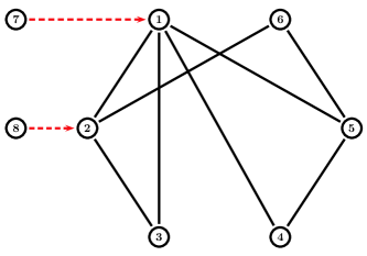
Figure 1: The communication graph.

Consider a network of eight agents with matching uncertainties. For illustration, let the communication graph among the agents be given as in Figure 1, where nodes 7 and 8 are two leaders and the others are followers. The dynamics of the agents are given by (1), with

$$x_{i}=\begin{bmatrix}x_{i1}\\ x_{i2}\end{bmatrix},\quad A=\begin{bmatrix}0&1\\ -1&1\end{bmatrix},\quad B=\begin{bmatrix}0\\ 1\end{bmatrix},$$

Design the control inputs for the leaders as $u_{7}=K_{7}x_{7}+4\sin(2t)$ and $u_{8}=K_{8}x_{8}+2\cos(t)$, with $K_{7}=-\begin{bmatrix}0&2\end{bmatrix}$ and $K_{8}=-\begin{bmatrix}1&3\end{bmatrix}$. It is easy to see that in this case $u_{7}$ and $u_{8}$ are bounded. Here we use the adaptive control (31) to solve the containment control problem.

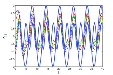
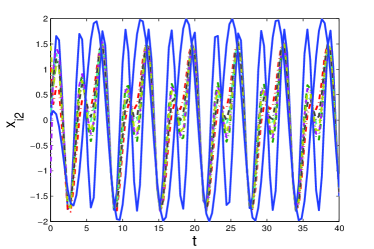
Figure 2: The state trajectories of the agents. The solid and dashdotted lines denote, respectively, the trajectories of the leaders and the followers.

Solving the LMI (9) by using the Sedumi toolbox [33] gives the gain matrices $K$ and $\Gamma$ in (31) as

$$K=-\begin{bmatrix}1.6203&4.7567\end{bmatrix},\quad\Gamma=\begin{bmatrix}2.6255&7.7075\\ 7.7075&22.6266\end{bmatrix}.$$

To illustrate Theorem 3, select $\kappa=0.1$, $\varphi_{i}=0.005$, and $\tau_{i}=5$, $i=2,\cdots,7$, in (31). The state trajectories $x_{i}(t)$ of the agents under (31) designed as above are depicted in Figure 2, implying that the containment control problem is indeed solved. The coupling gains $d_{i}$ associated with the followers are drawn in Figure 3, which are clearly bounded.

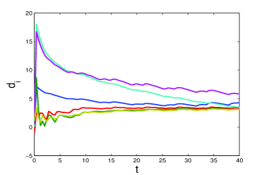
Figure 3: The coupling gains $d_{i}$ in (31).

7 Conclusion

In this paper, we have considered the containment control problem for multi-agent systems with general linear dynamics and multiple leaders whose control inputs are possibly nonzero and time varying. Based on the relative states and relative estimates of the states of neighboring agents, distributed static and adaptive continuous controllers have been designed, under which the containment error is uniformly ultimately bounded, if the subgraph associated with the followers is undirected and for each follower there exists at least one leader that has a directed path to that follower. A sufficient condition for the existence of these containment controllers is that each agent is stabilizable and detectable. An interesting future topic is to consider the distributed containment problem for the case with general directed communication graphs.

References

- [1] R. Olfati-Saber and R. Murray, “Consensus problems in networks of agents with switching topology and time-delays,” IEEE Transactions on Automatic Control, vol. 49, no. 9, pp. 1520–1533, 2004.
- [2] W. Ren, R. Beard, and E. Atkins, “Information consensus in multivehicle cooperative control,” IEEE Control Systems Magazine, vol. 27, no. 2, pp. 71–82, 2007.
- [3] A. Abdessameud and A. Tayebi, “On consensus algorithms for double-integrator dynamics without velocity measurements and with input constraints,” Systems & Control Letters, vol. 59, no. 12, pp. 812–821, 2010.
- [4] Z. Li, Z. Duan, G. Chen, and L. Huang, “Consensus of multiagent systems and synchronization of complex networks: A unified viewpoint,” IEEE Transactions on Circuits and Systems I: Regular Papers, vol. 57, no. 1, pp. 213–224, 2010.
- [5] Z. Li, Z. Duan, and G. Chen, “Dynamic consensus of linear multi-agent systems,” IET Control Theory and Applications, vol. 5, no. 1, pp. 19–28, 2011.
- [6] H. Zhang, F. Lewis, and A. Das, “Optimal design for synchronization of cooperative systems: State feedback, observer, and output feedback,” IEEE Transactions on Automatic Control, vol. 56, no. 8, pp. 1948–1952, 2011.
- [7] H. Zhang, M. Chen, and G. Stan, “Fast consensus via predictive pinning control,” IEEE Transactions on Circuits and Systems I: Regular Papers, vol. 58, no. 9, pp. 2247–2258, 2011.
- [8] K. You and L. Xie, “Network topology and communication data rate for consensusability of discrete-time multi-agent systems,” IEEE Transactions on Automatic Control, vol. 56, no. 10, pp. 2262–2275, 2011.
- [9] Z. Li, X. Liu, W. Ren, and L. Xie, “Distributed tracking control for linear multi-agent systems with a leader of bounded unknown input,” IEEE Transactions on Automatic Control, vol. 58, no. 2, pp. 518–523, 2013.
- [10] Z. Li, W. Ren, X. Liu, and L. Xie, “Distributed consensus of linear multi-agent systems with adaptive dynamic protocols,” Automatica, in press, 2013.
- [11] H. Grip, T. Yang, A. Saberi, and A. A. Stoorvogel, “Output synchronization for heterogeneous networks of non-introspective agents,” Automatica, vol. 48, no. 10, pp. 2444–2453, 2012.
- [12] M. Ji, G. Ferrari-Trecate, M. Egerstedt, and A. Buffa, “Containment control in mobile networks,” IEEE Transactions on Automatic Control, vol. 53, no. 8, pp. 1972–1975, 2008.
- [13] Y. Cao, D. Stuart, W. Ren, and Z. Meng, “Distributed containment control for multiple autonomous vehicles with double-integrator dynamics: Algorithms and experiments,” IEEE Transactions on Control Systems Technology, vol. 19, no. 4, pp. 929–938, 2011.
- [14] Y. Cao and W. Ren, “Containment control with multiple stationary or dynamic leaders under a directed interaction graph,” in Proceedings of the 48th IEEE Conference on Decision and Control and the 28th Chinese Control Conference, pp. 3014–3019, 2009.
- [15] Y. Cao, W. Ren, and M. Egerstedt, “Distributed containment control with multiple stationary or dynamic leaders in fixed and switching directed networks,” Automatica, vol. 48, no. 8, pp. 1586–1597, 2012.
- [16] Y. Lou and Y. Hong, “Target containment control of multi-agent systems with random switching interconnection topologies,” Automatica, vol. 48, no. 5, pp. 879–885, 2012.
- [17] L. Galbusera, G. Ferrari-Trecate, and R. Scattolini, “A hybrid model predictive control scheme for containment and distributed sensing in multi-agent systems,” Systems & Control Letters, vol. 62, no. 5, pp. 413–419, 2013.
- [18] J. Mei, W. Ren, and G. Ma, “Distributed containment control for lagrangian networks with parametric uncertainties under a directed graph,” Automatica, vol. 48, no. 4, pp. 653–659, 2012.
- [19] D. Dimarogonas, P. Tsiotras, and K. Kyriakopoulos, “Leader–follower cooperative attitude control of multiple rigid bodies,” Systems and Control Letters, vol. 58, no. 6, pp. 429–435, 2009.
- [20] Z. Meng, W. Ren, and Z. You, “Distributed finite-time attitude containment control for multiple rigid bodies,” Automatica, vol. 46, no. 12, pp. 2092–2099, 2010.
- [21] Z. Li, W. Ren, X. Liu, and M. Fu, “Distributed containment control of multi-agent systems with general linear dynamics in the presence of multiple leaders,” International Journal of Robust and Control, vol. 23, no. 5, pp. 534–547, 2013.
- [22] R. Agaev and P. Chebotarev, “On the spectra of nonsymmetric laplacian matrices,” Linear Algebra and its Applications, vol. 399, no. 1, pp. 157–178, 2005.
- [23] W. Ren and R. Beard, “Consensus seeking in multiagent systems under dynamically changing interaction topologies,” IEEE Transactions on Automatic Control, vol. 50, no. 5, pp. 655–661, 2005.
- [24] D. Shevitz and B. Paden, “Lyapunov stability theory of nonsmooth systems,” IEEE Transactions on Automatic Control, vol. 39, no. 9, pp. 1910–1914, 1994.
- [25] K. Young, V. Utkin, and U. Ozguner, “A control engineer’s guide to sliding mode control,” IEEE Transactions on Control Systems Technology, vol. 7, no. 3, pp. 328–342, 1999.
- [26] C. Edwards and S. Spurgeon, Sliding Mode Control: Theory and Applications. London: Taylor & Francis, 1998.
- [27] T. Yang, A. A. Stoorvogel, H. Grip, and A. Saberi, “Semi-global regulation of output synchronization for heterogeneous networks of non-introspective, invertible agents subject to actuator saturation,” International Journal of Robust and Nonlinear Control, in press, 2012.
- [28] Z. Meng, Z. Zhao, and Z. Lin, “On global leader-following consensus of identical linear dynamic systems subject to actuator saturation,” Systems & Control Letters, vol. 62, no. 2, pp. 132–142, 2013.
- [29] H. Khalil, Nonlinear Systems. Englewood Cliffs, NJ: Prentice Hall, 2002.
- [30] M. Corless and G. Leitmann, “Continuous state feedback guaranteeing uniform ultimate boundedness for uncertain dynamic systems,” IEEE Transactions on Automatic Control, vol. 26, no. 5, pp. 1139–1144, 1981.
- [31] P. Ioannou and P. Kokotovic, “Instability analysis and improvement of robustness of adaptive control,” Automatica, vol. 20, no. 5, pp. 583–594, 1984.
- [32] S. Boyd, L. El Ghaoui, E. Feron, and V. Balakrishnan, Linear Matrix Inequalities in System and Control Theory. Philadelphia, PA: SIAM, 1994.
- [33] J. Sturm, “Using SeDuMi 1.02, a MATLAB toolbox for optimization over symmetric cones,” Optimization Methods and Software, vol. 11, no. 1, pp. 625–653, 1999.