Multi-Layer Hydrostatic Equilibrium of Planets and Synchronous Moons: Theory and Application to Ceres and to Solar System Moons

Abstract

The hydrostatic equilibrium of multi-layer bodies lacks a satisfactory theoretical treatment despite its wide range of applicability. Here we show that by using the exact analytical potential of homogeneous ellipsoids we can obtain recursive analytical solutions and an exact numerical method for the hydrostatic equilibrium shape problem of multi-layer planets and synchronous moons. The recursive solutions rely on the series expansion of the potential in terms of the polar and equatorial shape eccentricities, while the numerical method uses the exact potential expression. These solutions can be used to infer the interior structure of planets and synchronous moons from the observed shape, rotation, and gravity. When applied to dwarf planet Ceres, we show that it is most likely a differentiated body with an icy crust of equatorial thickness 30–90 km and a rocky core of density 2.4–3.1 g/cm³. For synchronous moons, we show that the $J_{2}/C_{22}\simeq 10/3$ and the $(b-c)/(a-c)\simeq 1/4$ ratios have significant corrections of order $\Omega^{2}/(\pi G\rho)$, with important implications on how their gravitational coefficients are determined from flyby radio science data and on how we assess their hydrostatic equilibrium state.

1. Introduction

Understanding how gravity, pressure, and rotation contribute to the shape of a homogeneous fluid body has been a remarkable achievement, with many contributions over several centuries (Chandrasekhar, 1969). The homogeneous fluid body theory can be qualitatively applied to large planets and moons (Jeffreys, 1976), but their differentiated interior structure leads to significant deviations between theory and observations. The differentiation of large bodies is a natural consequence of radiogenic heating (Urey, 1955; MacPherson et al., 1995; Ghosh & McSween, 1998), causing partial or total melting and segregation of the heavier components towards the center of the body shortly after formation. Tidal dissipation can also represent an important heating source, as in the case of Io (Peale et al., 1979). This motivates us to investigate the hydrostatic equilibrium of multi-layer bodies.

The linear superposition of rotational and tidal deformations, which is a good approximation only for very slow rotators, led Dermott (1979) to compute the equilibrium figure of 2-layer planets and synchronous moons, including the deformation of the interior layer. A numerical 2-layer model by Thomas (1993) was used in Thomas et al. (2005) to determine the interior structure of Ceres, and we perform a similar analysis in §3. In Kong et al. (2010) the 2-layer problem for planets is approached using spheroidal coordinates, and this leads to implicit integral equations which are solved numerically, with realistic examples presented in Schubert et al. (2011). A recursive numerical form of the solution of the gravitational field of $N$-layer spheroids is presented in Hubbard (2013).

In this manuscript we show how the analytic expressions for the potential of a homogeneous ellipsoid can be used to obtain recursive high-order analytical solutions to the $N$-layer hydrostatic equilibrium problem, with closed-form 2nd order equations. Numerical methods can also be obtained with an accuracy which depends primarily on the precision of the floating point operations. Applications to Ceres and to synchronous moons of the giant planets are presented.

2. Methods

In an incompressible $N$-layer fluid body in hydrostatic equilibrium, pressure $p$, potential $U_{\text{tot}}$ and density $\rho$ satisfy the gradient equation

$$\nabla p=\rho\nabla U_{\text{tot}}$$ (1)

where the potential $U_{\text{tot}}$ has the form:

$$U_{\text{tot}} =U_{\text{rot}}+U_{\text{tid}}+\sum_{i=1}^{N}\frac{\rho_{i}-\rho_{i-1}}{\rho_{i}}U_{i}$$ (2)

$$U_{\text{rot}} =\frac{x^{2}+y^{2}}{2}\Omega^{2}$$ (3)

$$U_{\text{tid}} =\frac{2x^{2}-y^{2}-z^{2}}{2}\Omega^{2}$$ (4)

where $U_{\text{rot}}$ is the rotational potential in the body-fixed co-rotating frame, $\Omega=2\pi/T$ is the angular velocity, and $T$ is the rotation period. For synchronous moons, $U_{\text{tid}}$ is the leading term of the tidal potential (Murray and Dermott, 1999), where we have included only the static component. Rotation is about the $z$ axis, and for synchronous moons the perturbing planet is along the $x$ axis. We neglect the time-dependent component of the tidal potential as the moon is assumed to have negligible obliquity and to be on an orbit with negligible eccentricity. $U_{i}$ is the potential of the $i$-th layer, which is either $U_{\text{TE}}$, in the generic case of a triaxial ellipsoid, or $U_{\text{OS}}$ for oblate spheroids, with detailed expressions provided in the Appendix. Each layer $i$ is treated as a triaxial ellipsoid with semi-axes $a_{i}\geq b_{i}\geq c_{i}$, polar eccentricity $e_{pi}^{2}=1-(c_{i}/a_{i})^{2}$, equatorial eccentricity $e_{qi}^{2}=1-(b_{i}/a_{i})^{2}$, and density $\rho_{i}$. In the sum of Eq. (2), $i=1$ corresponds to the outer layer, and the density $\rho_{i}$ of each layer increases with $i$, while the layer size decreases so that the layer $i+1$ is fully contained in the layer $i$: $a_{i+1}\leq a_{i}$, $b_{i+1}\leq b_{i}$, $c_{i+1}\leq c_{i}$. Outside the body, the density is $\rho_{0}=0$. Finally, the contribution to $U_{\text{tot}}$ by each layer is proportional to its relative density increase, as expressed in the factor $(\rho_{i}-\rho_{i-1})/\rho_{i}$.

To solve the multi-layer hydrostatic equilibrium problem of Eqs. (1) and (2) and determine the semi-axes of all the layers, given their density and volume, it is sufficient to require that surfaces of constant density are equipotential. In this problem, equipotential surfaces are approximated by coaxial ellipsoids. This approximation is an excellent one: in the interior of an isolated layer the equipotential surfaces are exact ellipsoids, and as we show in Eq. (H6) in Appendix §H in the exterior of an isolated layer the deviation of an equipotential surface from an ellipsoid is very small and decreases very rapidly with distance, while it is identically zero along the principal axes. The rotational nature of the problem imposes to all layers to be coaxial. To verify that surfaces are equipotential it is then sufficient to compare the value of $U_{\text{tot}}$ at the three extremes along the principal axes.

2.1. Analytical Solutions

Analytical solutions of the multi-layer hydrostatic equilibrium problem can be obtained in the form of recursive relations. The principal idea of recursive equations originated while inverting the Maclaurin relation, which relates polar eccentricity $e_{p}$ and angular velocity $\Omega$ of a body with density $\rho$ in hydrostatic equilibrium (Chandrasekhar, 1969). As we show in Appendix §F, in the limit of small $e_{p}$ we can expand the Maclaurin relation in power series, and then obtain a recursive relation which effectively inverts the Maclaurin relation, providing $e_{p}$ as a function of $\Omega$ and $\rho$. In order to apply this approach to the multi-layer hydrostatic equilibrium problem, we use $U_{\text{tot}}$ from Eq. (2) where the potential $U_{i}$ of each layer is given by the power series expansions in Eq. (A3) and (A4). We then impose the condition for equipotential surfaces $U_{\text{tot}}(a_{i},0,0)=U_{\text{tot}}(0,b_{i},0)=U_{\text{tot}}(0,0,c_{i})$ and isolate the polar and equatorial eccentricities $e_{pi}$ and $e_{qi}$ in recursive relations.

2.1.1 Multi-Layer Planets

For a 2-layer planet, including terms up to the 2nd order in eccentricity in the gravitational potential from Eq. (A3) and (A4), we have:

$$e_{p1}^{2} \longleftarrow\frac{15\Lambda^{2}+12\mu_{2}^{5}\sigma_{2}e_{p2}^{2}}{8+20\mu_{2}^{3}\sigma_{2}}+\cdots$$ (5)

$$e_{p2}^{2} \longleftarrow\frac{15\Lambda^{2}+12e_{p1}^{2}}{20+8\sigma_{2}}+\cdots$$ (6)

where $\mu_{i}=a_{i}/a_{1}$, $\sigma_{i}=(\rho_{i}-\rho_{i-1})/\rho_{1}$, $\Lambda^{2}=\Omega^{2}/(\pi G\rho_{1})$, $G$ is the gravitational constant, and we have $\mu_{1}=1$, $\sigma_{1}=1$. The left hand eccentricities in Eq. (5) and (6) are iteratively updated with the value of the expressions on the right, with initial values $e_{pi}=0$. Higher order recursive relations are provided in Appendix §G. For a 3-layer planet, the 2nd order recursive equations are:

$$e_{p1}^{2} \longleftarrow\frac{15\Lambda^{2}+12\mu_{2}^{5}\sigma_{2}e_{p2}^{2}+12\mu_{3}^{5}\sigma_{3}e_{p3}^{2}}{8+20\mu_{2}^{3}\sigma_{2}+20\mu_{3}^{3}\sigma_{3}}+\cdots$$ (7)

$$e_{p2}^{2} \longleftarrow\frac{15\Lambda^{2}+12e_{p1}^{2}+12(\mu_{3}/\mu_{2})^{5}\sigma_{3}e_{p3}^{2}}{20+8\sigma_{2}+20(\mu_{3}/\mu_{2})^{3}\sigma_{3}}+\cdots$$ (8)

$$e_{p3}^{2} \longleftarrow\frac{15\Lambda^{2}+12e_{p1}^{2}+12\sigma_{2}e_{p2}^{2}}{20+20\sigma_{2}+8\sigma_{3}}+\cdots$$ (9)

For a $N$-layer planet the general recursive relation for the $i$-th layer is then:

$$e_{pi}^{2} \longleftarrow\frac{\displaystyle 15\Lambda^{2}+12\sum_{k=1}^{i-1}\sigma_{k}e_{pk}^{2}+12\sum_{k=i+1}^{N}(\mu_{k}/\mu_{i})^{5}\sigma_{k}e_{pk}^{2}}{\displaystyle 20\sum_{k=1}^{i-1}\sigma_{k}+8\sigma_{i}+20\sum_{k=i+1}^{N}(\mu_{k}/\mu_{i})^{3}\sigma_{k}}+\cdots$$ (10)

where the sums are to account for the effects of outer ($k<i$) and inner ($k>i$) layers relative to the $i$-th layer considered. Once the shape of each layer has been determined, we can obtain the inertia moments from Appendix §D and the expansion of the gravitational potential from Appendix §C.

The 2nd order recursive equations above converge to closed form equations, which can be obtained by solving for the $N$ unknowns $e_{pi}$ the system of $N$ linearly independent equations $U_{\text{tot}}(a_{i},0,0)=U_{\text{tot}}(0,0,c_{i})$. The 2-layer 2nd order solution in Eq. (5) and (6) converges to the closed form

$$e_{p1}^{2} =\frac{15\Lambda^{2}}{8}\frac{(1+(2/5)\sigma_{2}+(3/5)\mu_{2}^{5}\sigma_{2})}{F_{p}}$$ (11)

$$e_{p2}^{2} =\frac{15\Lambda^{2}}{8}\frac{(1+\mu_{2}^{3}\sigma_{2})}{F_{p}}$$ (12)

where

$$F_{p}=1+(2/5)\sigma_{2}+(5/2)\mu_{2}^{3}\sigma_{2}+\mu_{2}^{3}\sigma_{2}^{2}-(9/10)\mu_{2}^{5}\sigma_{2}$$

For the ratio of the eccentricities, we have:

$$\frac{e_{p2}^{2}}{e_{p1}^{2}} =\frac{1+\mu_{2}^{3}\sigma_{2}}{1+(2/5)\sigma_{2}+(3/5)\mu_{2}^{5}\sigma_{2}}$$ (13)

which is non-zero even in the limit of a small core:

$$\frac{e_{p2}^{2}}{e_{p1}^{2}} \xrightarrow{\mu_{2}\to 0}\frac{5\rho_{1}}{3\rho_{1}+2\rho_{2}}\leq 1$$ (14)

The expressions for the $J_{2}=-C_{20}$ gravity coefficient and the principal moment of inertia $C$ are then:

$$J_{2} =\frac{3\Lambda^{2}}{8}\frac{(1+(2/5)\sigma_{2}+(8/5)\mu_{2}^{5}\sigma_{2}+\mu_{2}^{8}\sigma_{2}^{2})}{(1+\mu_{2}^{3}\sigma_{2})F_{p}}$$ (15)

$$\begin{split}\frac{C}{Ma_{1}^{2}}&=\frac{2}{5}\frac{(1+\mu_{2}^{5}\sigma_{2})}{(1+\mu_{2}^{3}\sigma_{2})}\\ &-\frac{3\Lambda^{2}}{20}\frac{\mu_{2}^{3}\sigma_{2}^{2}(1-\mu_{2}^{2}-(5/2)\mu_{2}^{3}+4\mu_{2}^{5}-(3/2)\mu_{2}^{7})}{(1+\mu_{2}^{3}\sigma_{2})^{2}F_{p}}\end{split}$$ (16)

The upper bounds can be obtained in the limit of an homogeneous body ($\sigma_{2}\to 0$), and are $e_{p1}\leq(15/8)\Lambda^{2}$, $J_{2}\leq(3/8)\Lambda^{2}$ and $C/(Ma_{1}^{2})\leq 2/5$.

2.1.2 Multi-Layer Synchronous Moons

The presence of a tidal potential causes non-zero equatorial eccentricities $e_{qi}$, and for a 2-layer synchronous moon, including terms up to the 2nd order in eccentricity, we have:

$$e_{p1}^{2} \longleftarrow\frac{60\Lambda^{2}+12\mu_{2}^{5}\sigma_{2}e_{p2}^{2}}{8+20\mu_{2}^{3}\sigma_{2}}+\cdots$$ (17)

$$e_{p2}^{2} \longleftarrow\frac{60\Lambda^{2}+12e_{p1}^{2}}{20+8\sigma_{2}}+\cdots$$ (18)

$$e_{q1}^{2} \longleftarrow\frac{45\Lambda^{2}+12\mu_{2}^{5}\sigma_{2}e_{q2}^{2}}{8+20\mu_{2}^{3}\sigma_{2}}+\cdots$$ (19)

$$e_{q2}^{2} \longleftarrow\frac{45\Lambda^{2}+12e_{q1}^{2}}{20+8\sigma_{2}}+\cdots$$ (20)

Higher order recursive relations are provided in Appendix §G. For a 3-layer synchronous moon, the 2nd order recursive equations are:

$$e_{p1}^{2} \longleftarrow\frac{60\Lambda^{2}+12\mu_{2}^{5}\sigma_{2}e_{p2}^{2}+12\mu_{3}^{5}\sigma_{3}e_{p3}^{2}}{8+20\mu_{2}^{3}\sigma_{2}+20\mu_{3}^{3}\sigma_{3}}+\cdots$$ (21)

$$e_{p2}^{2} \longleftarrow\frac{60\Lambda^{2}+12e_{p1}^{2}+12(\mu_{3}/\mu_{2})^{5}\sigma_{3}e_{p3}^{2}}{20+8\sigma_{2}+20(\mu_{3}/\mu_{2})^{3}\sigma_{3}}+\cdots$$ (22)

$$e_{p3}^{2} \longleftarrow\frac{60\Lambda^{2}+12e_{p1}^{2}+12\sigma_{2}e_{p2}^{2}}{20+20\sigma_{2}+8\sigma_{3}}+\cdots$$ (23)

$$e_{q1}^{2} \longleftarrow\frac{45\Lambda^{2}+12\mu_{2}^{5}\sigma_{2}e_{q2}^{2}+12\mu_{3}^{5}\sigma_{3}e_{q3}^{2}}{8+20\mu_{2}^{3}\sigma_{2}+20\mu_{3}^{3}\sigma_{3}}+\cdots$$ (24)

$$e_{q2}^{2} \longleftarrow\frac{45\Lambda^{2}+12e_{q1}^{2}+12(\mu_{3}/\mu_{2})^{5}\sigma_{3}e_{q3}^{2}}{20+8\sigma_{2}+20(\mu_{3}/\mu_{2})^{3}\sigma_{3}}+\cdots$$ (25)

$$e_{q3}^{2} \longleftarrow\frac{45\Lambda^{2}+12e_{q1}^{2}+12\sigma_{2}e_{q2}^{2}}{20+20\sigma_{2}+8\sigma_{3}}+\cdots$$ (26)

For a $N$-layer synchronous moon the general recursive relation for the $i$-th layer is then:

$$e_{pi}^{2} \longleftarrow\frac{\displaystyle 60\Lambda^{2}+12\sum_{k=1}^{i-1}\sigma_{k}e_{pk}^{2}+12\sum_{k=i+1}^{N}(\mu_{k}/\mu_{i})^{5}\sigma_{k}e_{pk}^{2}}{\displaystyle 20\sum_{k=1}^{i-1}\sigma_{k}+8\sigma_{i}+20\sum_{k=i+1}^{N}(\mu_{k}/\mu_{i})^{3}\sigma_{k}}+\cdots$$ (27)

$$e_{qi}^{2} \longleftarrow\frac{\displaystyle 45\Lambda^{2}+12\sum_{k=1}^{i-1}\sigma_{k}e_{qk}^{2}+12\sum_{k=i+1}^{N}(\mu_{k}/\mu_{i})^{5}\sigma_{k}e_{qk}^{2}}{\displaystyle 20\sum_{k=1}^{i-1}\sigma_{k}+8\sigma_{i}+20\sum_{k=i+1}^{N}(\mu_{k}/\mu_{i})^{3}\sigma_{k}}+\cdots$$ (28)

Similarly to §2.1.1 the 2nd order recursive equations admit closed form solutions, and the 2-layer 2nd order solution in Eq. (5) and (6) converges to

$$e_{p1}^{2} =\frac{15\Lambda^{2}}{2}\frac{(1+(2/5)\sigma_{2}+(3/5)\mu_{2}^{5}\sigma_{2})}{F_{p}}$$ (29)

$$e_{p2}^{2} =\frac{15\Lambda^{2}}{2}\frac{(1+\mu_{2}^{3}\sigma_{2})}{F_{p}}$$ (30)

$$e_{q1}^{2} =\frac{45\Lambda^{2}}{8}\frac{(1+(2/5)\sigma_{2}+(3/5)\mu_{2}^{5}\sigma_{2})}{F_{p}}$$ (31)

$$e_{q2}^{2} =\frac{45\Lambda^{2}}{8}\frac{(1+\mu_{2}^{3}\sigma_{2})}{F_{p}}$$ (32)

Note how the polar eccentricities in Eqs. (29)–(30) and the equatorial eccentricities in Eqs. (31)–(32) are respectively a factor 4 and a factor 3 larger than the rotation-only polar eccentricities in Eqs. (11)–(12) for the corresponding layer, a result originally attributed to Clairaut.

The expressions for the $J_{2}$ and $C_{22}$ gravity coefficients and the principal moment of inertia $C$ are:

$$J_{2} =\frac{15\Lambda^{2}}{16}\frac{(1+(2/5)\sigma_{2}+(8/5)\mu_{2}^{5}\sigma_{2}+\mu_{2}^{8}\sigma_{2}^{2})}{(1+\mu_{2}^{3}\sigma_{2})F_{p}}$$ (33)

$$C_{22} =\frac{9\Lambda^{2}}{32}\frac{(1+(2/5)\sigma_{2}+(8/5)\mu_{2}^{5}\sigma_{2}+\mu_{2}^{8}\sigma_{2}^{2})}{(1+\mu_{2}^{3}\sigma_{2})F_{p}}$$ (34)

$$\frac{C}{Ma_{1}^{2}} =\frac{2}{5}\frac{(1+\mu_{2}^{5}\sigma_{2})}{(1+\mu_{2}^{3}\sigma_{2})}-\frac{9\Lambda^{2}}{8}\frac{G_{C}}{(1+\mu_{2}^{3}\sigma_{2})^{2}F_{p}}$$ (35)

where

$$G_{C} =1+(2/5)\sigma_{2}+\mu_{2}^{3}\sigma_{2}+(8/5)\mu_{2}^{5}\sigma_{2}+(4/3)\mu_{2}^{3}\sigma_{2}^{2}$$

$$-(14/15)\mu_{2}^{5}\sigma_{2}^{2}-(7/3)\mu_{2}^{6}\sigma_{2}^{2}+(19/3)\mu_{2}^{8}\sigma_{2}^{2}$$

$$-(7/5)\mu_{2}^{10}\sigma_{2}^{2}+\mu_{2}^{11}\sigma_{2}^{3}$$

The upper bounds given by $\sigma_{2}\to 0$ are $e_{p1}\leq(15/2)\Lambda^{2}$, $e_{q1}\leq(45/8)\Lambda^{2}$, $J_{2}\leq(15/16)\Lambda^{2}$, and $C_{22}\leq(9/32)\Lambda^{2}$. For $C/(Ma_{1}^{2})$ we have that it is smaller than the homogeneous moon value of $(2/5)-(9/8)\Lambda^{2}$ for most values of $\mu_{2}$ except when $\mu_{2}\simeq 1$, in which case $(2/5)-(9/8)\Lambda^{2}\leq C/(Ma_{1}^{2})\leq 2/5$.

2.2. Numerical Solutions

For fast-rotating multi-layer planets and synchronous moons the polar and equatorial eccentricities $e_{pi}$ and $e_{qi}$ obtained with analytical methods in §2.1 tend to converge very slowly to the exact solution, even when using high-order recursive equations, see Table 2 in §2.3. Additionally, the Maclaurin equation includes disk-like solutions with $e_{pi}\simeq 1$ (Chandrasekhar, 1969) which are beyond the range of applicability of methods based on power series expansion of the potential. To overcome these limitations, we have included a numerical method capable of finding all the admissible solutions, including the high $e_{pi}$ ones and the Jacobi branch for triaxial ellipsoid solutions of planets.

In the numerical method we use $U_{\text{tot}}$ from Eq. (2) where the potential $U_{i}$ of each layer is given by the exact analytic expressions in Eq. (A1) and (B1). We then impose the condition for equipotential surfaces $U_{\text{tot}}(a_{i},0,0)=U_{\text{tot}}(0,b_{i},0)=U_{\text{tot}}(0,0,c_{i})$ by performing numerical minimization of $\Delta^{2}$:

$$\begin{split}\Delta^{2}&=\sum_{k=1}^{N}\left[U_{\text{tot}}(0,b_{i},0)-U_{\text{tot}}(a_{i},0,0)\right]^{2}\\ &+\sum_{k=1}^{N}\left[U_{\text{tot}}(0,0,c_{i})-U_{\text{tot}}(a_{i},0,0)\right]^{2}\end{split}$$ (36)

and solve for the polar and equatorial eccentricities $e_{pi}$ and $e_{qi}$. The accuracy of the solution depends on the precision of the floating point operations, including the effect of roundoff errors. Satisfactory solutions will have $\Delta^{2}$ compatible with zero within the numerical precision. The initial values of $e_{pi}$ and $e_{qi}$ in general can be chosen at random between 0 and 1, or can be seeded using the 2nd order recursive relations in Eq. (10) for planets or in Eq. (27) and (28) for synchronous moons when applicable.

2.3. Comparison with Previous Works

Our analytical and numerical solutions are now compared to previous results in the literature. In Kong et al. (2010) the 2-layer problem is studied in spheroidal coordinates, and numerical solutions are obtained along with some test cases. In particular, we use their Figure 4 test case to perform a direct comparison with our solutions. Note that in Kong et al. (2010) the convention for layer numbering is inverted with respect to ours. In the 2-layer model, the polar eccentricity of each layer is determined while varying the relative volume fraction of the core $Q_{V}=\mu_{2}^{3}(1-e_{p2}^{2})^{1/2}(1-e_{p1}^{2})^{-1/2}$ from 0 to 1, at a fixed density ratio $\rho_{2}/\rho_{1}=2$, or $\sigma_{2}=1$. The rotation is fixed at $\Lambda^{2}=\Omega^{2}/(\pi G\rho_{1})=2\varepsilon_{2}$ with $\varepsilon_{2}=0.05$.

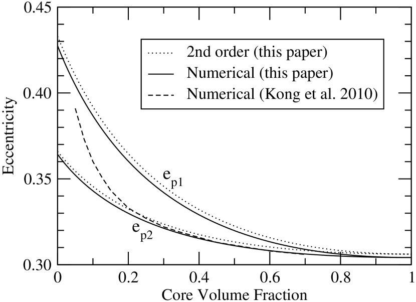
Figure 1.— Comparison of 2-layer solutions with Fig. 4 in Kong et al. (2010). The numerical solutions are indistinguishable for $e_{p1}$, while they are significantly different for $e_{p2}$ for a small core.

In Figure 1 we show our results along with that of Kong et al. (2010). If we take our numerical solutions as reference, our 2nd order analytical solution is within approximately 1%, and the 4th order solution is within approximately 0.01% and is not displayed in Figure 1 because indistinguishable from the numerical one. Our numerical values for the eccentricity of the outer layer $e_{p1}$ are in very good agreement with Kong et al. (2010) over the whole range of core volume fraction, including the two limiting values of 0.4275 (no core) and 0.3042 (all core). However, for the eccentricity of the inner layer $e_{p2}$ we have good agreement only in the limit of a large core, while for a small core the solution of Kong et al. (2010) seems to significantly over-estimate the core eccentricity, reaching a relative difference of over 10% at $Q_{V}=0.05$.

Additional test cases are presented in Schubert et al. (2011), including their Figure 2 with the eccentricity of equipotential surfaces plotted against the equatorial radius.

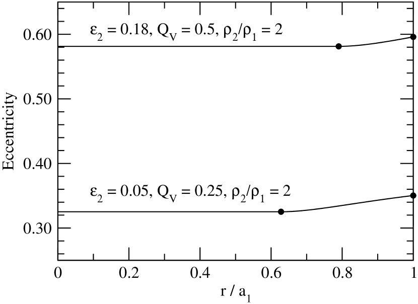
Figure 2.— Our 2-layer solutions for the test case described in Fig. 2 of Schubert et al. (2011). The dots represent the equatorial radius and eccentricity of each layer.

Our results for this case are displayed in Figure 2, where we have that the eccentricity of equipotential surfaces is constant within the core and then grows monotonically, in contrast with what found by Schubert et al. (2011) who describe significant oscillations in proximity of the interface and a general decrease when moving towards the center of the body. In support of our results we have the following argument, which applies in general to any number of layers and to both the rotational and tidal cases: from Eq. (2) we have that the total potential in the innermost layer is given by the exact expressions for $U_{\text{TE,in}}$ or $U_{\text{OS,in}}$ (in the Appendix) for each layer, plus the rotational and tidal components, and as such the total potential it is quadratic in the cartesian coordinates with constant factors, because $\kappa=0$, so it generates equipotential surfaces with constant $e_{p}$ and $e_{q}$.

Test Case	$Q_{V}$	$\rho_{1}/\rho_{2}$	$\varepsilon_{2}$
Mars	0.125	0.486	0.00347
Neptune	0.091125	0.157334	0.0254179
Uranus 2	0.0563272	0.0791231	0.0318902

Table 1Test cases and corresponding numerical constants used as input.

Test Case	Method	$e_{p1}$	$e_{p2}$	$J_{2}\times 10^{6}$
Mars	Schubert et al. (2011)	0.100 30	0.088 859	1823.1
Mars	Zharkov & Trubitsyn (1978)	0.100 295	0.088 874 7	1823.18
Mars	Hubbard (2013)	0.100 294 71	0.088 874 693	1823.183 2
Mars	2nd order (this paper)	0.100 384	0.088 918	1826.2
Mars	4th order (this paper)	0.100 291 836	0.088 869 977	1822.871
Mars	6th order (this paper)	0.100 291 642 754	0.088 870 801 531	1822.865 533
Mars	Numerical (this paper)	0.100 291 642 478 822	0.088 870 803 521 489	1822.865 525 162
Neptune	Schubert et al. (2011)	0.210 19	0.151 47	6241.0
Neptune	Zharkov & Trubitsyn (1978)	0.209 658	0.143 515	6188.92
Neptune	Hubbard (2013)	0.209 658 98	0.143 515 34	6188.926 7
Neptune	2nd order (this paper)	0.211 151	0.143 688	6264.3
Neptune	4th order (this paper)	0.209 638 699	0.143 443 899	6177.9
Neptune	6th order (this paper)	0.209 599 221 310	0.143 453 888 914	6175.757 821
Neptune	Numerical (this paper)	0.209 597 812 191 680	0.143 453 902 049 024	6175.678 534 586
Uranus 2	Schubert et al. (2011)	0.214 73	0.141 60	5801.4
Uranus 2	Zharkov & Trubitsyn (1978)	0.213 648	0.115 655	5680.32
Uranus 2	Hubbard (2013)	0.213 648 98	0.115 655 64	5680.324 2
Uranus 2	2nd order (this paper)	0.215 683	0.115 731	5773.8
Uranus 2	4th order (this paper)	0.213 642 242	0.115 593 114	5667.7
Uranus 2	6th order (this paper)	0.213 578 684	0.115 596 690 381	5664.394 033
Uranus 2	Numerical (this paper)	0.213 576 194 544 737	0.115 596 602 475 207	5664.265 380 457

Table 2 The shape of the two layers is computed using several methods for the test cases in Table 1. The Schubert et al. (2011) values are computed using the method by Kong et al. (2010). Zharkov & Trubitsyn (1978) refers to 3rd order values as computed by Schubert et al. (2011) using the theory in Zharkov & Trubitsyn (1978). Our values are obtained using the recursive formulas with orders 2 to 6 described in §2.1 and Appendix §G, and then using the numerical method described in §2.2. Using our numerical values as reference, which should be exact to the last digit (no rounding), we have underlined the digits which agree with it, to roughly assess their accuracy.

$Q_{V}$	$\rho_{1}/\rho_{2}$	$\varepsilon_{2}$	Method	$e_{p1}$	$e_{p2}$	$e_{q1}$	$e_{q2}$
0.1	0.5	0.001	2nd order	0.110 686	0.097 654	0.095 857	0.084 570
0.1	0.5	0.001	4th order	0.110 548 762	0.097 590 596	0.095 952 320	0.084 682 230
0.1	0.5	0.001	Numerical	0.110 548 771 238	0.097 591 141 031	0.095 953 221 967	0.084 683 153 224
0.2	0.3	0.01	2nd order	0.275 437	0.233 621	0.238 535	0.202 322
0.2	0.3	0.01	4th order	0.272 764 535	0.232 579 902	0.239 444 944	0.203 668 851
0.2	0.3	0.01	Numerical	0.272 712 086 703	0.232 608 245 285	0.239 498 516 335	0.203 734 133 006

Table 3Similar to Table 2 but for 2-layer synchronous moons. All three methods are from this paper: 2nd order from §2.1.2, 4th order from Appendix §G, and numerical from §2.2.

Additionally, several 2-layer test cases are used both in Schubert et al. (2011) and in Hubbard (2013), so we include a Table to provide our estimates along theirs. The input values used in each test case are listed in Table 1 and the results in Table 2. We find that our analytical and numerical approaches are in very good agreement with each other, with the recursive values approaching the numerical ones as the order of the analytical expressions increases. We find the values computed using the methods in Zharkov & Trubitsyn (1978) and Hubbard (2013) show consistently an accuracy better than our 2nd order but worse than our 4th order solutions. In comparison, the results of Schubert et al. (2011) have an inconsistent accuracy: better than our 2nd order but worse than our 4th order solutions for the Mars case, which has the larger core and the slowest rotation of the three cases, but otherwise significantly worse than our 2nd order solutions for the Neptune and Uranus 2 cases. Overall we consider satisfactory the agreement of our solutions with Zharkov & Trubitsyn (1978) and with Hubbard (2013) but find the method by Kong et al. (2010) to suffer from significant inaccuracies in the limit of a small core. We note that the theory in Kong et al. (2010) explicitly distinguishes between small core and large core, so it is entirely possible that the small core theory shows issues while leaving the large core theory unaffected.

Finally, in Table 3 we provide a few 2-layer test cases for synchronous moons, which can be used as benchmark and future reference, since we could not find similar cases to compare to in the literature.

3. Ceres

Ceres is the largest main-belt object, to be visited in 2015 by the Dawn mission (Russell et al., 2007). Its low density and fast rotation cause a significant polar flattening, consistent with the shape of an oblate spheroid, as determined by stellar occultation (Millis et al., 1987), HST observations (Thomas et al., 2005), and Keck AO observations (Carry et al., 2008). The shape determination by Thomas et al. (2005) in particular is based on a full longitudinal coverage of Ceres’ rotation, and measured the semi-axes $a=487.3\pm 1.8$ km and $c=454.7\pm 1.6$ km. The mass of Ceres has been measured by Baer & Chesley (2008) in the context of gravitational perturbations by large main-belt asteroids in astrometric data, obtaining $(4.75\pm 0.03)\times 10^{-10}$ $M_{\text{Sun}}$, in agreement with previous estimates (Michalak, 2000; Standish, 2001; Pitjeva, 2005; Konopliv et al., 2006). The bulk density is then $2.09\pm 0.02$ g/cm³. The rotation period of $9.074170\pm 0.000002$ h was measured by Chamberlain et al. (2007) using lightcurve data covering a period of almost 50 years.

We have performed a forward modeling Monte Carlo, using 2-layer (core, crust) and 3-layer (core, mantle, crust) numerical models and uniformly sampling the density and volume of each layer. The numerical approach was preferred to avoid the small errors introduced by analytic solutions, see §2.3 and Table 2. We impose on each solution the hydrostatic equilibrium condition and determine the exterior shape. The resulting shape semi-axes $a$ and $c$ and total mass of Ceres of each solution are then compared to the observed values using the $\chi^{2}$ statistics with 3 degrees of freedom and confidence level CL of 0.50 or 0.95, the former to determine the parameters of the model which most closely match the nominal shape and mass of Ceres, the latter to find a wider range of parameters which are more broadly compatible with the observations.

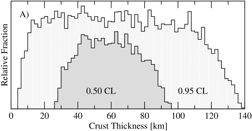
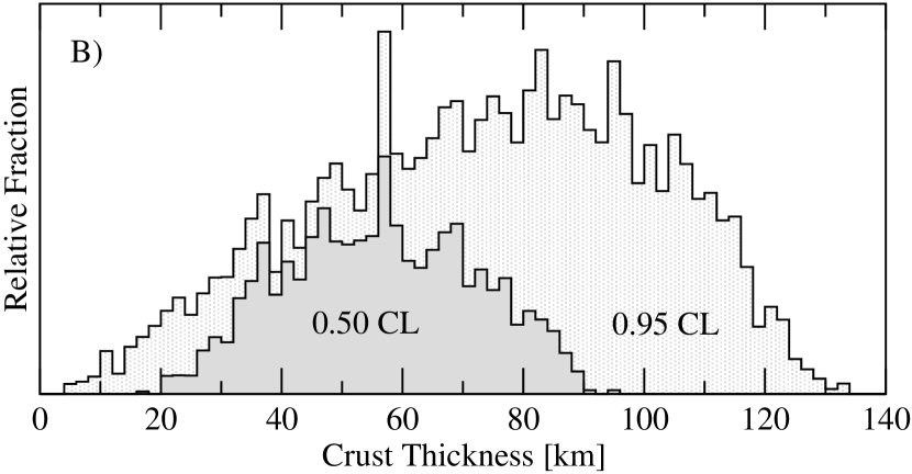
Figure 3.— Distribution of Ceres 2-layer (A) and 3-layer (B) model solutions versus thickness of the water-ice crust, at a confidence level (CL) of 0.50 (dark grey) and 0.95 (light grey). The relative fraction is the ratio of the number of solutions in each bin with the number of baseline solutions in the same bin, and is in arbitrary linear units.

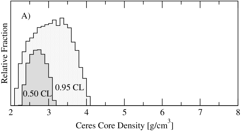
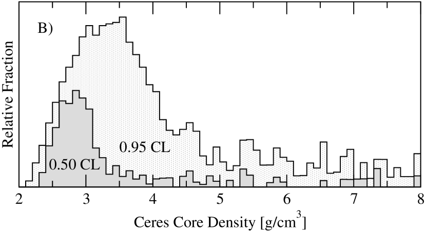
Figure 4.— Distribution of Ceres 2-layer (A) and 3-layer (B) model solutions versus core density, same conventions as Figure 3.

Solutions are selected according to our general understanding of the composition of Ceres (McCord & Sotin, 2005; Thomas et al., 2005; Zolotov, 2009; Castillo-Rogez & McCord, 2010). The outer crust is assumed to be water-ice, with a density of 0.90–0.95 g/cm³ (Lide, 2005), allowing for a small margin for possible porosity or impurities. The mantle is assumed to be rocky, with a density of 2.1–3.5 g/cm³. The core is allowed to have a density of 2.1–8.0 g/cm³, from a light rocky core up to a possible metallic core. For Monte Carlo normalization purposes, we also select a baseline set of solutions with global density 0.9–8.0 g/cm³ and 0.99 CL. For the 2-layer model, a total of 309,814 solutions were included in the baseline set, with 7,971 included in the 0.95 CL set, and 2,885 included in the 0.50 CL set. For the 3-layer model, a total of 459,662 solutions were included in the baseline set, with 3,279 included in the 0.95 CL set, and 1,223 included in the 0.50 CL set.

We find that interior solutions are not compatible with a homogeneous Ceres at 0.95 CL, in agreement with Thomas et al. (2005). Most of the 2-layer and 3-layer solutions at 0.50 CL show a crust thickness approximately 30–90 km, see Fig. 3, and a core density 2.4–3.1 g/cm³, see Fig. 4. At 0.95 CL the two models show more different solutions: a crust thickness 5–130 km for the 2-layer model, and 20–120 km for the 3-layer model; a core density 2.2–4.0 g/cm³ for the 2-layer model, and 2.4–4.7 g/cm³ for the 3-layer model. Most 3-layer solutions have a small density difference between core and mantle, typically smaller than 1.0 g/cm³, which may indicate different levels of hydration (Castillo-Rogez & McCord, 2010). A low tail of solutions with a metallic core is present in 3-layer solutions at 0.95 CL, which becomes negligible at 0.50 CL. In Fig. 5 we show a scatter plot of the resulting $J_{2}$ gravity coefficients and normalized principal inertia moment $C$.

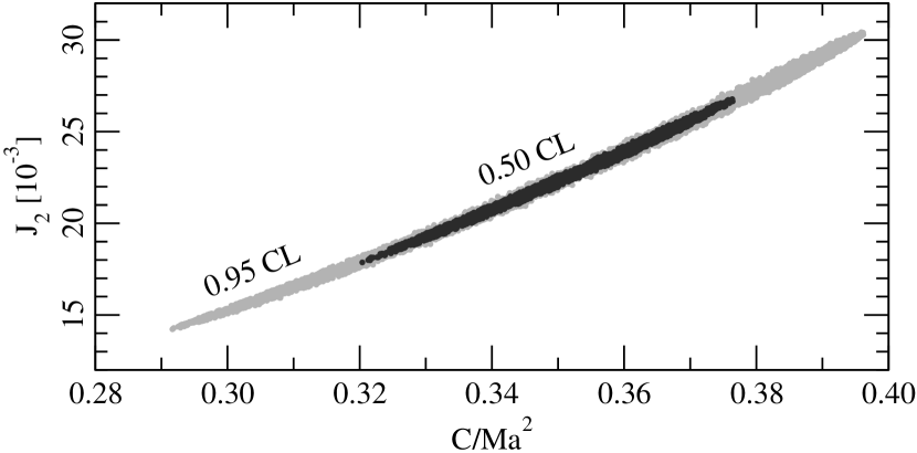
Figure 5.— Scatter plot of the $J_{2}$ gravity coefficient versus normalized principal moment of inertia $C/Ma^{2}$ for Ceres solutions, which have virtually identical distributions for the 2-layer and the 3-layer models. The 0.50 and 0.95 CL solutions are marked by black and grey regions, respectively.

4. Solar System Moons

This method can be applied to solar system moons, and in Figure 6 we have plotted the minimum value of the $J_{2}/C_{22}$ and $(b-c)/(a-c)$ ratios for selected bulk density values, and included the estimated value for several large and fast-rotating moons of the giant planets of the solar system. These values are computed numerically using the observed rotation period and bulk density. For reference, the asymptotic values of $J_{2}/C_{22}=10/3$ and $(b-c)/(a-c)=1/4$ are given by the dotted line.

The decrease of the ratio $(b-c)/(a-c)$ for fast rotators was already present in Chandrasekhar (1969) and noted in Dermott & Thomas (1988). The analytical dependence to order $\Lambda^{2}$ of the ratios $J_{2}/C_{22}$ and $(b-c)/(a-c)$ can be obtained using the relations in Eq. (G3) to (G6), and in the limit of an homogeneous synchronous moon ($\sigma_{2}\to 0$) we obtain the compact expressions:

$$e_{p1}^{2} =\frac{15}{2}\Lambda^{2}-\frac{1125}{112}\Lambda^{4}+\cdots$$ (37)

$$e_{q1}^{2} =\frac{45}{8}\Lambda^{2}+\frac{3375}{448}\Lambda^{4}+\cdots$$ (38)

and the ratio

$$\frac{b-c}{a-c} =\frac{1}{4}-\frac{1485}{896}\Lambda^{2}+\cdots$$ (39)

while for the gravity coefficients we have

$$J_{2} =\frac{15}{16}\Lambda^{2}-\frac{2475}{896}\Lambda^{4}+\cdots$$ (40)

$$C_{22} =\frac{9}{32}\Lambda^{2}+\frac{675}{1792}\Lambda^{4}+\cdots$$ (41)

with the ratio

$$\frac{J_{2}}{C_{22}} =\frac{10}{3}-\frac{100}{7}\Lambda^{2}+\cdots$$ (42)

These expressions for the ratios to order $\Lambda^{2}$ are good approximations for all solar system moons, with the largest relative error of about 1% for Mimas and much smaller for all the other moons, see Figure 6.

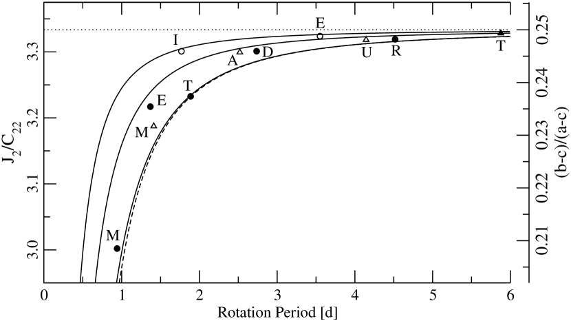
Figure 6.— Minimum equilibrium values for the $J_{2}/C_{22}$ and $(b-c)/(a-c)$ ratios versus rotation period. The solid curves show the numerical solution for homogeneous synchronous moons of density 1, 2, and 4 g/cm³. The dashed curve shows the approximated solution from Eq. (39) and (42) for density 1 g/cm³. Moons of Jupiter^a (open circle): Io, Europa. Moons of Saturn^b (solid circle): Mimas, Enceladus, Tethys, Dione, Rhea. Moons of Uranus^c (open triangle): Miranda, Ariel, Umbriel. Moons of Neptune^d (solid triangle): Triton. References for bulk density data: ^aSchubert et al. (2004); ^bThomas (2010); ^cJacobson et al. (1992); ^dThomas (2000).

5. Discussion

We suggest a Ceres icy crust thickness of 30–90 km, which is in good agreement with thermal evolution scenarios by McCord & Sotin (2005) and Castillo-Rogez & McCord (2010). Thomas et al. (2005) determine an icy crust thickness of 66–124 km using a 2-layer model, which tends to be larger than the values suggested here. This may be due to the modeling of the shape of the interior layers, and it is not clear how the method by Thomas (1993) which is used in Thomas et al. (2005) deals with this issue. Our core density estimate of 2.4–3.1 g/cm³ agrees with the 2.7 g/cm³ by Thomas et al. (2005).

The $J_{2}/C_{22}$ ratio in synchronous moons is often constrained a-priori to its nominal value of $10/3$ when determining the individual gravity coefficients from flyby radio science data (Anderson et al., 2003; Schubert et al., 2004; Anderson & Schubert, 2007; Mackenzie et al., 2008; Anderson & Schubert, 2010). As we show in Eq. (42) and Fig. 6, the value of $J_{2}/C_{22}$ has a significant correction due to fast rotation, and this should be taken into account when determining the gravity coefficients. A similar correction is present in the $(b-c)/(a-c)$ ratio, see Eq. (39) and Fig. 6.

The shape of planets and synchronous moons is expected to viscously relax and asymptotically reach the equilibrium shape, which may or may not be reached within the age of the solar system depending on how effective the relaxation process is (Johnson & McGetchin, 1973). Of six well-measured Saturnian large icy moons, three (Tethys, Dione, Rhea) have clearly interpretable equilibrium shapes, and the other three (Mimas, Enceladus, Iapetus) appear to be significantly off hydrostatic equilibrium (Thomas et al., 2007; Thomas, 2010), and this can be due to their formation mechanisms, as well as their thermal, dynamical, rotational, and collisional history. The analytical and numerical solutions presented can help us assess how far moons are from hydrostatic equilibrium, potentially providing an insight on the different scenarios leading to their current shapes.

6. Conclusions

The analytical and numerical solutions presented in this manuscript mark a clear improvement over previous methods. The 2nd order recursive analytical relations in Eq. (10) for planets and in Eq. (27) and (28) for synchronous moons apply to an arbitrary number of layers, and express in a very compact form how the shape of each layer is a generalized weighted average of the shapes of all the other layers, with the relative sizes and densities as weights, plus a source term proportional to $\Omega^{2}$. High-order relations can be obtained for bodies with a small number of layers, as we did for 2-layer bodies in Appendix §G. Finally, the numerical method allows to obtain solutions which are exact within the precision of the floating point operations, and converge for slow- and fast-rotating bodies, up to a number of layers which is essentially limited by the processing power available.

Our results have important applications to solar system planets and synchronous moons. For planets, accounting for the deformation of each layer is a significant improvement over previous models, and when applied to Ceres, it generates solutions which have a water-ice crust thinner than previously thought. For synchronous moons, we model the deformation due to rotation and tidal effects jointly, extending the range of applicability of analytical solutions to moderately fast rotators, and obtaining 2nd order analytical expressions for the $J_{2}/C_{22}$ and $(b-c)/(a-c)$ ratios.

Appendix A Gravitational Potential of a Homogeneous Triaxial Ellipsoid

The gravitational potential of an homogeneous triaxial ellipsoid (TE) is analytic (MacMillan, 1930):

$$\begin{split}\frac{U_{\text{TE}}(x,y,z)}{\pi G\rho}&=\frac{2abc}{\sqrt{a^{2}-c^{2}}}\left[1-\frac{x^{2}}{a^{2}-b^{2}}+\frac{y^{2}}{a^{2}-b^{2}}\right]F(\psi,e_{q}^{2}/e_{p}^{2})\\ &+\frac{2abc}{\sqrt{a^{2}-c^{2}}}\left[\frac{x^{2}}{a^{2}-b^{2}}-\frac{(a^{2}-c^{2})y^{2}}{(a^{2}-b^{2})(b^{2}-c^{2})}+\frac{z^{2}}{b^{2}-c^{2}}\right]E(\psi,e_{q}^{2}/e_{p}^{2})\\ &+\frac{2abc}{\sqrt{(a^{2}+\kappa)(b^{2}+\kappa)(c^{2}+\kappa)}}\left[\frac{c^{2}+\kappa}{b^{2}-c^{2}}y^{2}-\frac{b^{2}+\kappa}{b^{2}-c^{2}}z^{2}\right]\end{split}$$ (A1)

where $\sin^{2}(\psi)=(a^{2}-c^{2})/(a^{2}+\kappa)$, $F$ and $E$ are the elliptic integral functions of the first and second kind, respectively. The variable $\kappa$ is the positive root of the equation

$$\frac{x^{2}}{a^{2}+\kappa}+\frac{y^{2}}{b^{2}+\kappa}+\frac{z^{2}}{c^{2}+\kappa}=1$$ (A2)

for points $(x,y,z)$ outside the ellipsoid, and $\kappa=0$ inside. The expansion for $e_{p}\ll 1$ is:

$$\begin{split}\frac{U_{\text{TE,in}}(x,y,z)}{\pi G\rho}&=\frac{2}{3}(3a^{2}-r^{2})-\frac{2}{15}(5a^{2}-r^{2}+3z^{2})e_{p}^{2}-\frac{2}{15}(5a^{2}-r^{2}+3y^{2})e_{q}^{2}\\ &-\frac{2}{105}(14a^{2}-4r^{2}+12z^{2})e_{p}^{4}+\frac{2}{105}(14a^{2}+r^{2}-3x^{2})e_{p}^{2}e_{q}^{2}-\frac{2}{105}(14a^{2}-4r^{2}+12y^{2})e_{q}^{4}+\cdots\end{split}$$ (A3)

$$\begin{split}\frac{U_{\text{TE,out}}(x,y,z)}{\pi G\rho}&=\frac{4a^{3}}{3r}-\frac{2a^{3}\left[5r^{4}-a^{2}(r^{2}-3z^{2})\right]}{15r^{5}}e_{p}^{2}-\frac{2a^{3}\left[5r^{4}-a^{2}(r^{2}-3y^{2})\right]}{15r^{5}}e_{q}^{2}\\ &-\frac{a^{3}\left[35r^{8}+14a^{2}r^{4}(r^{2}-3z^{2})-3a^{4}(3x^{4}+6x^{2}(y^{2}-4z^{2})+3y^{4}-24y^{2}z^{2}+8z^{4})\right]}{210r^{9}}e_{p}^{4}\\ &+\frac{a^{3}\left[35r^{8}+7a^{2}r^{4}(-2x^{2}+y^{2}+z^{2})+3a^{4}(x^{4}-3x^{2}(y^{2}+z^{2})-4y^{4}+27y^{2}z^{2}-4z^{4})\right]}{105r^{9}}e_{p}^{2}e_{q}^{2}\\ &-\frac{a^{3}\left[35r^{8}+14a^{2}r^{4}(r^{2}-3y^{2})-3a^{4}(3x^{4}+6x^{2}(z^{2}-4y^{2})+3z^{4}-24y^{2}z^{2}+8y^{4})\right]}{210r^{9}}e_{q}^{4}+\cdots\end{split}$$ (A4)

where $r^{2}=x^{2}+y^{2}+z^{2}$ and the potential is continuous with continuous derivative at the surface of the triaxial ellipsoid. For $\kappa$ we have:

$$\kappa =r^{2}-a^{2}+\frac{a^{2}z^{2}}{r^{2}}e_{p}^{2}+\frac{a^{2}y^{2}}{r^{2}}e_{q}^{2}+\frac{a^{4}(x^{2}+y^{2})z^{2}}{r^{6}}e_{p}^{4}-2\frac{a^{4}y^{2}z^{2}}{r^{6}}e_{p}^{2}e_{q}^{2}+\frac{a^{4}(x^{2}+z^{2})y^{2}}{r^{6}}e_{q}^{4}+\cdots$$ (A5)

and a recursive formula can be obtained simply by extracting a $\kappa$ factor from Eq. (A2):

$$\kappa \longleftarrow\frac{x^{2}}{1+a^{2}/\kappa}+\frac{y^{2}}{1+b^{2}/\kappa}+\frac{z^{2}}{1+c^{2}/\kappa}$$ (A6)

and using $\kappa=r^{2}-a^{2}$ as initial value.

Appendix B Gravitational Potential of a Homogeneous Oblate Spheroid

The gravitational potential takes a simpler form in the case of oblate spheroids (OS), where $e_{q}=0$ (MacMillan, 1930):

$$\begin{split}\frac{U_{\text{OS}}(x,y,z)}{\pi G\rho}&=\frac{2a^{2}c}{\sqrt{a^{2}-c^{2}}}\left[1-\frac{r^{2}-3z^{2}}{2(a^{2}-c^{2})}\right]\psi+\frac{a^{2}c}{a^{2}-c^{2}}\left[\frac{\sqrt{c^{2}+\kappa}}{a^{2}+\kappa}(x^{2}+y^{2})-\frac{2z^{2}}{\sqrt{c^{2}+\kappa}}\right]\end{split}$$ (B1)

and the expansion of $U_{\text{OS}}$ for $e_{p}\ll 1$ can be recovered directly from the $U_{\text{TE}}$ expressions in Eq. (A3) and (A4) by simply setting $e_{q}=0$.

Appendix C Spherical Harmonics

The gravitational potential of an homogeneous triaxial ellipsoid can be expanded in spherical harmonics (Kaula, 1966; Yoder, 1995) to obtain:

$$U=\frac{GM}{r}\left[1+\sum_{l=2}^{\infty}\sum_{m=0}^{l}\frac{a_{1}^{l}}{r^{l}}C_{lm}P_{lm}(\cos(\theta))\cos(m\phi)\right]$$ (C1)

where $P_{lm}(\cos(\theta))$ is the associate Legendre function, $\cos(\theta)=z/r$ and $\tan\phi=y/x$. This series converges absolutely outside the sphere with reference radius $a_{1}$, and the unnormalized coefficients $C_{lm}$ can be determined by integrating over the volume of the body (MacMillan, 1930; Yoder, 1995). The coefficients are (MacMillan, 1930; Yoder, 1995; Tricarico, 2008):

$$\begin{split}C_{lm}&=\frac{(2-\delta_{0m})}{2^{l}}\frac{(l-m)!}{(l+m)!}\sum_{p=0}^{l/2}\sum_{q=0}^{m/2}(-1)^{p+q}\binom{l}{p}\binom{2l-2p}{l}\binom{m}{2q}\\ &(l-m-2p+1)_{m}\sum_{\nu_{x}=0}^{p}\sum_{\nu_{y}=0}^{p-\nu_{x}}\frac{p!}{\nu_{x}!\nu_{y}!(p-\nu_{x}-\nu_{y})!}{\cal N}_{m-2q+2\nu_{x},2q+2\nu_{y},l-m-2\nu_{x}-2\nu_{y}}\end{split}$$ (C2)

where both $l$ and $m$ are even, and $C_{lm}=0$ otherwise. The generalized moments of inertia coefficients ${\cal N}_{n_{x}n_{y}n_{z}}$ are:

$${\cal N}_{n_{x}n_{y}n_{z}} =\frac{3}{4\pi}\dfrac{\Gamma\left[(n_{x}+1)/2\right]\Gamma\left[(n_{y}+1)/2\right]\Gamma\left[(n_{z}+1)/2\right]}{\Gamma\left[(n_{x}+n_{y}+n_{z}+5)/2\right]}(1-e_{q}^{2})^{n_{y}/2}(1-e_{p}^{2})^{n_{z}/2}$$ (C3)

if $n_{x},n_{y},n_{z}$ are all even, and ${\cal N}_{n_{x}n_{y}n_{z}}=0$ otherwise. The non-zero $C_{lm}$ terms for $l\leq 4$ are:

$$C_{20} =\frac{(e_{q}^{2}-2e_{p}^{2})}{10} C_{22} =\frac{e_{q}^{2}}{20} C_{40} =\frac{3(8e_{p}^{4}-8e_{p}^{2}e_{q}^{2}+3e_{q}^{4})}{280} C_{42} =\frac{(e_{q}^{4}-2e_{p}^{2}e_{q}^{2})}{280} C_{44} =\frac{e_{q}^{4}}{2240}$$ (C4)

and in the special case of an oblate spheroid ($e_{q}=0$) we have that only the $C_{l0}$ terms with even $l$ are non-zero, with

$$C_{l0} =(-1)^{l/2}\frac{3}{(l+1)(l+3)}e_{p}^{l}$$ (C5)

and using the convention $J_{l}=-C_{l0}$ we have

$$J_{2} =\frac{1}{5}e_{p}^{2} J_{4} =-\frac{3}{35}e_{p}^{4} J_{6} =\frac{1}{21}e_{p}^{6} J_{8} =-\frac{1}{33}e_{p}^{8} J_{10} =\frac{3}{143}e_{p}^{10}$$ (C6)

When computing the $C_{lm}$ for a multi-layer body, we have to include the relative size factor $a_{i}^{l}/a_{1}^{l}$ to refer all contributions to the same exterior semi-axis $a_{1}$, and also scale by the mass fraction $M_{i}/M=V_{i}(\rho_{i}-\rho_{i-1})/M$ contributed by the layer, with $V_{i}=(4\pi/3)a_{i}^{3}(1-e_{pi}^{2})^{1/2}(1-e_{qi}^{2})^{1/2}$ volume of the layer, and $M=\sum_{i=1}^{N}M_{i}=\sum_{i=1}^{N}V_{i}(\rho_{i}-\rho_{i-1})$ total mass of the body, to obtain $C_{lm}=\sum_{i=1}^{N}(a_{i}/a_{1})^{l}(M_{i}/M)C_{lm,i}$ where $C_{lm,i}$ is the single layer $C_{lm}$ from Eq. (C2).

Appendix D Inertia Moments

The principal moments of inertia $A,B,C$ for a homogeneous ellipsoid are:

$$\frac{A}{Ma_{1}^{2}} =\frac{2-e_{p1}^{2}-e_{q1}^{2}}{5} \frac{B}{Ma_{1}^{2}} =\frac{2-e_{p1}^{2}}{5} \frac{C}{Ma_{1}^{2}} =\frac{2-e_{q1}^{2}}{5}$$ (D1)

and when combining it in a multi-layer body, we have:

$$\frac{A}{Ma_{1}^{2}} =\sum_{i=1}^{N}\frac{a_{i}^{2}}{a_{1}^{2}}\frac{M_{i}}{M}\frac{(2-e_{pi}^{2}-e_{qi}^{2})}{5} \frac{B}{Ma_{1}^{2}} =\sum_{i=1}^{N}\frac{a_{i}^{2}}{a_{1}^{2}}\frac{M_{i}}{M}\frac{(2-e_{pi}^{2})}{5} \frac{C}{Ma_{1}^{2}} =\sum_{i=1}^{N}\frac{a_{i}^{2}}{a_{1}^{2}}\frac{M_{i}}{M}\frac{(2-e_{qi}^{2})}{5}$$ (D2)

Appendix E Pressure

The interior pressure $p$ of a multi-layer body in hydrostatic equilibrium can be obtained from Eq. (1):

$$p(x,y,z)=\sum_{i=1}^{N(x,y,z)}(\rho_{i}-\rho_{i-1})\left[U_{\text{tot}}(x,y,z)-U_{\text{tot}}(a_{i},0,0)\right]$$ (E1)

where the sum is over the $N(x,y,z)$ layers containing the point $(x,y,z)$.

Appendix F Inverse Maclaurin Relation

The angular velocity $\Omega$ and polar eccentricity $e_{p}$ of a rotating homogeneous fluid body in hydrostatic equilibrium follow the exact relation (Chandrasekhar, 1969)

$$\frac{\Omega^{2}}{\pi G\rho} =\Lambda^{2}=\frac{(1-e_{p}^{2})^{1/2}}{e_{p}^{3}}2(3-2e_{p}^{2})\arcsin(e_{p})-\frac{6}{e_{p}^{2}}(1-e_{p}^{2})$$ (F1)

which can be expanded in power series for $e_{p}\ll 1$ as

$$\Lambda^{2} =\frac{8}{15}e_{p}^{2}+\frac{8}{105}e_{p}^{4}-\frac{64}{3465}e_{p}^{8}-\frac{1024}{45045}e_{p}^{10}+\cdots$$ (F2)

and this relation can be inverted using a recursive scheme

$$e_{p}^{2} \longleftarrow\frac{15}{8}\left[\Lambda^{2}-\frac{8}{105}e_{p}^{4}+\frac{64}{3465}e_{p}^{8}+\frac{1024}{45045}e_{p}^{10}+\cdots\right]$$ (F3)

where the value of $e_{p}^{2}$ on the left side of Eq. (F3) is successively improved by substituting the value of the expression on the right side. Starting with $e_{p}^{2}=0$, we get $e_{p}^{2}=(15/8)\Lambda^{2}$ after the first iteration, and after five iterations we have:

$$e_{p}^{2} =\frac{15}{8}\Lambda^{2}-\frac{225}{448}\Lambda^{4}+\frac{3375}{12544}\Lambda^{6}+\frac{3830625}{15454208}\Lambda^{8}+\frac{349565625}{803618816}\Lambda^{10}+\cdots$$ (F4)

Appendix G High-Order Recursive Solutions

The equations in recursive form including 6th order eccentricity terms for a 2-layer planet are

$$\begin{split}e_{p1}^{2}&\longleftarrow\frac{15\Lambda^{2}+12\mu_{2}^{5}\sigma_{2}e_{p2}^{2}}{8+20\mu_{2}^{3}\sigma_{2}}-\frac{(8+105\mu_{2}^{3}\sigma_{2})e_{p1}^{4}-(70\mu_{2}^{3}+84\mu_{2}^{5})\sigma_{2}e_{p1}^{2}e_{p2}^{2}+(42\mu_{2}^{5}+15\mu_{2}^{7})\sigma_{2}e_{p2}^{4}}{7(8+20\mu_{2}^{3}\sigma_{2})}\\ &\phantom{\longleftarrow}-\frac{175\mu_{2}^{3}\sigma_{2}e_{p1}^{6}-(105\mu_{2}^{3}+210\mu_{2}^{5})\sigma_{2}e_{p1}^{4}e_{p2}^{2}-(35\mu_{2}^{3}-84\mu_{2}^{5}-120\mu_{2}^{7})\sigma_{2}e_{p1}^{2}e_{p2}^{4}+(21\mu_{2}^{5}-15\mu_{2}^{7}-35\mu_{2}^{9})\sigma_{2}e_{p2}^{6}}{14(8+20\mu_{2}^{3}\sigma_{2})}+\cdots\end{split}$$ (G1)

$$\begin{split}e_{p2}^{2}&\longleftarrow\frac{15\Lambda^{2}+12e_{p1}^{2}}{20+8\sigma_{2}}+\frac{48e_{p1}^{4}-56e_{p1}^{2}e_{p2}^{2}-8\sigma_{2}e_{p2}^{4}}{7(20+8\sigma_{2})}+\frac{32e_{p1}^{6}}{7(20+8\sigma_{2})}+\cdots\end{split}$$ (G2)

For a 2-layer synchronous moon we have the 4th order expansion:

$$\begin{split}e_{p1}^{2}&\longleftarrow\frac{60\Lambda^{2}+12\mu_{2}^{5}\sigma_{2}e_{p2}^{2}}{8+20\mu_{2}^{3}\sigma_{2}}-\frac{(22+140\mu_{2}^{3}\sigma_{2})e_{p1}^{4}-(70\mu_{2}^{3}+105\mu_{2}^{5})\sigma_{2}e_{p1}^{2}e_{p2}^{2}+(42\mu_{2}^{5}+15\mu_{2}^{7})\sigma_{2}e_{p2}^{4}}{7(8+20\mu_{2}^{3}\sigma_{2})}\\ &\phantom{\longleftarrow}+\frac{16e_{p1}^{2}e_{q1}^{2}+(70\mu_{2}^{3}-42\mu_{2}^{5})\sigma_{2}e_{p1}^{2}e_{q2}^{2}-(42\mu_{2}^{5}-30\mu_{2}^{7})\sigma_{2}e_{p2}^{2}e_{q2}^{2}}{7(8+20\mu_{2}^{3}\sigma_{2})}+\cdots\end{split}$$ (G3)

$$e_{p2}^{2} \longleftarrow\frac{60\Lambda^{2}+12e_{p1}^{2}}{20+8\sigma_{2}}+\frac{48e_{p1}^{4}-35e_{p1}^{2}e_{p2}^{2}-(35+22\sigma_{2})e_{p2}^{4}}{7(20+8\sigma_{2})}-\frac{12e_{p1}^{2}e_{q1}^{2}-28e_{q1}^{2}e_{p2}^{2}-16\sigma_{2}e_{p2}^{2}e_{q2}^{2}}{7(20+8\sigma_{2})}+\cdots$$ (G4)

$$\begin{split}e_{q1}^{2}&\longleftarrow\frac{45\Lambda^{2}+12\mu_{2}^{5}\sigma_{2}e_{q2}^{2}}{8+20\mu_{2}^{3}\sigma_{2}}-\frac{(8+105\mu_{2}^{3}\sigma_{2})e_{q1}^{4}+(42\mu_{2}^{5}+15\mu_{2}^{7})\sigma_{2}e_{q2}^{4}}{7(8+20\mu_{2}^{3}\sigma_{2})}\\ &\phantom{\longleftarrow}+\frac{16e_{p1}^{2}e_{q1}^{2}+(70\mu_{2}^{3}-42\mu_{2}^{5})\sigma_{2}e_{q1}^{2}e_{p2}^{2}+(70\mu_{2}^{3}+84\mu_{2}^{5})\sigma_{2}e_{q1}^{2}e_{q2}^{2}-(42\mu_{2}^{5}-30\mu_{2}^{7})\sigma_{2}e_{p2}^{2}e_{q2}^{2}}{7(8+20\mu_{2}^{3}\sigma_{2})}+\cdots\end{split}$$ (G5)

$$e_{q2}^{2} \longleftarrow\frac{45\Lambda^{2}+12e_{q1}^{2}}{20+8\sigma_{2}}+\frac{48e_{q1}^{4}-8\sigma_{2}e_{q2}^{4}}{7(20+8\sigma_{2})}-\frac{12e_{p1}^{2}e_{q1}^{2}+56e_{q1}^{2}e_{q2}^{2}-28e_{p1}^{2}e_{q2}^{2}-16\sigma_{2}e_{p2}^{2}e_{q2}^{2}}{7(20+8\sigma_{2})}+\cdots$$ (G6)

Appendix H Equipotential Surface Outside an Homogeneous Triaxial Ellipsoid

An homogeneous triaxial ellipsoid with semi-major axis $a_{1}$ and polar and equatorial eccentricities $e_{p1}$ and $e_{q1}$ generates an equipotential surface at its exterior, which can be approximated by triaxial ellipsoid with semi-major axis $a_{0}>a_{1}$ and eccentricities $e_{p0}$ and $e_{q0}$. By using Eq. (A4) and imposing $U_{\text{TE,out}}(a_{0},0,0)=U_{\text{TE,out}}(0,b_{0},0)=U_{\text{TE,out}}(0,0,c_{0})$ we can obtain the 4th order recursive expressions

$$e_{p0}^{2} \longleftarrow\frac{3}{5}\frac{a_{1}^{2}}{a_{0}^{2}}e_{p1}^{2}+\frac{177}{700}\frac{a_{1}^{4}}{a_{0}^{4}}e_{p1}^{4}+\frac{6}{175}\frac{a_{1}^{4}}{a_{0}^{4}}e_{p1}^{2}e_{q1}^{2}-\frac{3}{4}e_{p0}^{4}+\cdots$$ (H1)

$$e_{q0}^{2} \longleftarrow\frac{3}{5}\frac{a_{1}^{2}}{a_{0}^{2}}e_{q1}^{2}+\frac{177}{700}\frac{a_{1}^{4}}{a_{0}^{4}}e_{q1}^{4}+\frac{6}{175}\frac{a_{1}^{4}}{a_{0}^{4}}e_{p1}^{2}e_{q1}^{2}-\frac{3}{4}e_{q0}^{4}+\cdots$$ (H2)

which do not depend on the density or angular velocity of the homogeneous ellipsoid, and converge to

$$e_{p0}^{2} =\frac{3}{5}\frac{a_{1}^{2}}{a_{0}^{2}}e_{p1}^{2}-\frac{3}{175}\frac{a_{1}^{4}}{a_{0}^{4}}e_{p1}^{4}+\frac{6}{175}\frac{a_{1}^{4}}{a_{0}^{4}}e_{p1}^{2}e_{q1}^{2}+\cdots$$ (H3)

$$e_{q0}^{2} =\frac{3}{5}\frac{a_{1}^{2}}{a_{0}^{2}}e_{q1}^{2}-\frac{3}{175}\frac{a_{1}^{4}}{a_{0}^{4}}e_{q1}^{4}+\frac{6}{175}\frac{a_{1}^{4}}{a_{0}^{4}}e_{p1}^{2}e_{q1}^{2}+\cdots$$ (H4)

The equipotential surface is close to but not exactly an ellipsoid, and using spherical coordinates $(x,y,z)=\left(r\sin(\theta)\cos(\phi),r\sin(\theta)\sin(\phi),r\cos(\theta)\right)$ we can calculate the ratio $\eta={r_{U}}/{r_{E}}$, where $r_{U}$ is the radius of the equipotential surface which is obtained by imposing $U_{\text{TE,out}}(x,y,z)=U_{\text{TE,out}}(a_{0},0,0)$, while $r_{E}$ is the radius of the ellipsoid

$$\frac{1}{r_{E}^{2}} =\frac{\sin^{2}(\theta)\cos^{2}(\phi)}{a_{0}^{2}}+\frac{\sin^{2}(\theta)\sin^{2}(\phi)}{a_{0}^{2}(1-e_{q0}^{2})}+\frac{\cos^{2}(\theta)}{a_{0}^{2}(1-e_{p0}^{2})}$$ (H5)

The expression for $\eta$ is then

$$\eta =1-\frac{3}{200}\frac{a_{1}^{4}}{a_{0}^{4}}\left[\sin^{2}(2\theta)e_{p1}^{4}-2\sin^{2}(2\theta)\sin^{2}(\phi)e_{p1}^{2}e_{q1}^{2}+\left(3+\cos(2\theta)+2\cos(2\phi)\sin^{2}(\theta)\right)\sin^{2}(\theta)\sin^{2}(\phi)e_{q1}^{4}\right]+\cdots$$ (H6)

showing that the deviation of the equipotential surface from the reference ellipsoid includes only terms of 4th order in eccentricity or higher, and decreases as the 4th power of the distance. Also, we have that $\eta\leq 1$ which means that the equipotential surface is in general just interior to the reference ellipsoid. In particular, $\eta=1$ at the extremes of the principal axes for a triaxial ellipsoid, while for an oblate spheroid $\eta=1$ at the poles and at the equator.

The minimum of $\eta$ is in the limit of $a_{0}\to a_{1}$ and shows a complex angular dependence. For a homogeneous rotating planet in hydrostatic equilibrium, with $e_{p1}$ from Eq. (F4) and $e_{q1}=0$, we have that $\eta$ from Eq. (H6) becomes

$$\eta =1-\frac{27}{512}\frac{a_{1}^{4}}{a_{0}^{4}}\sin^{2}(2\theta)\Lambda^{4}+\cdots$$ (H7)

with equal minima at $\theta=\pi/4$ and at $\theta=3\pi/4$, which correspond to latitudes of $\pm 45^{\circ}$. For an homogeneous synchronous moon in hydrostatic equilibrium, with $e_{p1}$ from Eq. (37) and $e_{q1}$ from Eq. (38), we have that $\eta$ from Eq. (H6) becomes

$$\eta =1-\frac{27}{2048}\frac{a_{1}^{4}}{a_{0}^{4}}\left[(77+59\cos(2\theta))\sin^{2}(\theta)-18\sin^{4}(\theta)\cos(4\phi)+30\sin^{2}(2\theta)\cos(2\phi)\right]\Lambda^{4}+\cdots$$ (H8)

with equal minima along the 4 specularly symmetric directions $(\theta,\phi)=\left\{(\pi/4,0),(\pi/4,\pi),(3\pi/4,0),(3\pi/4,\pi)\right\}$ where

$$\eta =1-\frac{27}{32}\frac{a_{1}^{4}}{a_{0}^{4}}\Lambda^{4}+\cdots$$ (H9)

References

• Anderson et al. (2003) Anderson, J. D., Rappaport, N. J., Giampieri, G., Schubert, G., & Moore, W. B. 2003, Physics of the Earth and Planetary Interiors, 136, 201
• Anderson & Schubert (2007) Anderson, J. D., & Schubert, G. 2007, Geophys. Res. Lett., 34, 2202
• Anderson & Schubert (2010) Anderson, J. D., & Schubert, G. 2010, Physics of the Earth and Planetary Interiors, 178, 176
• Baer & Chesley (2008) Baer, J., & Chesley, S. R. 2008, Celestial Mechanics and Dynamical Astronomy, 100, 27
• Carry et al. (2008) Carry, B., Dumas, C., Fulchignoni, M., et al. 2008, A&A, 478, 235
• Castillo-Rogez & McCord (2010) Castillo-Rogez, J. C., & McCord, T. B. 2010, Icarus, 205, 443
• Chamberlain et al. (2007) Chamberlain, M. A., Sykes, M. V., & Esquerdo, G. A. 2007, Icarus, 188, 451
• Chandrasekhar (1969) Chandrasekhar, S. 1969, Ellipsoidal Figures of Equilibrium, Yale University Press
• Dermott (1979) Dermott, S. F. 1979, Icarus, 37, 575
• Dermott & Thomas (1988) Dermott, S. F., & Thomas, P. C. 1988, Icarus, 73, 25
• Ghosh & McSween (1998) Ghosh, A., & McSween, H. Y. 1998, Icarus, 134, 187
• Hubbard (2013) Hubbard, W. B. 2013, ApJ, 768, 43
• Jacobson et al. (1992) Jacobson, R. A., Campbell, J. K., Taylor, A. H., & Synnott, S. P. 1992, AJ, 103, 2068
• Jeffreys (1976) Jeffreys, H. 1976, The Earth. Its origin, history and physical constitution. Cambridge University Press
• Johnson & McGetchin (1973) Johnson, T. V., & McGetchin, T. R. 1973, Icarus, 18, 612
• Kaula (1966) Kaula, W. M. 1966. Theory of satellite geodesy. Applications of satellites to geodesy. Blaisdell.
• Kong et al. (2010) Kong, D., Zhang, K., & Schubert, G. 2010, Journal of Geophysical Research (Planets), 115, 12003
• Konopliv et al. (2006) Konopliv, A. S., Yoder, C. F., Standish, E. M., Yuan, D.-N., & Sjogren, W. L. 2006, Icarus, 182, 23
• Lide (2005) Lide, D. R. 2005, CRC Handbook of Chemistry and Physics, CRC Press
• Mackenzie et al. (2008) Mackenzie, R. A., Iess, L., Tortora, P., & Rappaport, N. J. 2008, Geophys. Res. Lett., 35, 5204
• MacMillan (1930) MacMillan, W. D. 1930. The Theory of the Potential. McGraw-Hill Book Co.
• MacPherson et al. (1995) MacPherson, G. J., Davis, A. M., & Zinner, E. K. 1995, Meteoritics, 30, 365
• McCord & Sotin (2005) McCord, T. B., & Sotin, C. 2005, Journal of Geophysical Research (Planets), 110, 5009
• Michalak (2000) Michalak, G. 2000, A&A, 360, 363
• Millis et al. (1987) Millis, R. L., Wasserman, L. H., Franz, O. G., et al. 1987, Icarus, 72, 507
• Murray and Dermott (1999) Murray, C. D., Dermott, S. F. 1999. Solar system dynamics. Cambridge University Press
• Peale et al. (1979) Peale, S. J., Cassen, P., & Reynolds, R. T. 1979, Science, 203, 892
• Pitjeva (2005) Pitjeva, E. V. 2005, Solar System Research, 39, 176
• Russell et al. (2007) Russell, C. T., Capaccioni, F., Coradini, A., et al. 2007, Earth Moon and Planets, 101, 65
• Schubert et al. (2004) Schubert, G., Anderson, J. D., Spohn, T., & McKinnon, W. B. 2004, Jupiter. The Planet, Satellites and Magnetosphere, 281
• Schubert et al. (2011) Schubert, G., Anderson, J., Zhang, K., Kong, D., & Helled, R. 2011, Physics of the Earth and Planetary Interiors, 187, 364
• Standish (2001) Standish, E. M. 2001. Technical Report 312.F-01-006, JPL Interoffice Memorandum
• Thomas (1993) Thomas, P. C. 1993, Icarus, 105, 326
• Thomas (2000) Thomas, P. C. 2000, Icarus, 148, 587
• Thomas et al. (2005) Thomas, P. C., Parker, J. W., McFadden, L. A., et al. 2005, Nature, 437, 224
• Thomas et al. (2007) Thomas, P. C., Burns, J. A., Helfenstein, P., et al. 2007, Icarus, 190, 573
• Thomas (2010) Thomas, P. C. 2010, Icarus, 208, 395
• Tricarico (2008) Tricarico, P. 2008, Celestial Mechanics and Dynamical Astronomy, 100, 319
• Urey (1955) Urey, H. C. 1955, Proceedings of the National Academy of Science, 41, 127
• Yoder (1995) Yoder, C. F. 1995. Astrometric and Geodetic Properties of Earth and the Solar System. Global Earth Physics: A Handbook of Physical Constants 1.
• Zharkov & Trubitsyn (1978) Zharkov, V. N., & Trubitsyn, V. P. 1978, Physics of planetary interiors, Pachart Press.
• Zolotov (2009) Zolotov, M. Y. 2009, Icarus, 204, 183