UA-NPPS/BSM-2-13

Six-dimensional origin of gravity mediated brane to brane supersymmetry breaking
G. A.  Diamandis,   B. C.  Georgalas,   P.  Kouroumalou and

A. B.  Lahanas

University of Athens,
Physics Department, Nuclear and Particle Physics Section,
GR–15771 Athens, Greece

Four dimensional supergravities may be the right framework to describe particle physics at low energies. Its connection to the underlying string theory can be implemented through higher dimensional supergravities which bear special characteristics. Their reduction to four dimensions breaks supersymmetry whose magnitude depends both on the compactifying manifold and the mechanism that generates the breaking. In particular compactifications, notably on a $S_{1}/Z_{2}$ orbifold, the breaking of supersymmetry occuring on a hidden brane, residing at one end of $S_{1}/Z_{2}$, is communicated to the visible brane which lies at the other end, via gravitational interactions propagating in the bulk. This scenario has been exemplified in the framework of the $N=2$, $D=5$ supergravity. In this note, motivated by the recent developments in the field, related to the six-dimensional description of the supergravity theory, we study the $N=2$, $D=5$ supergravity theory as originating from a $D=6$ supergravity which, in addition to the gravity, includes a number of tensor multiplets. This reduces to $N=1$, $D=4$ supergravity in a two step manner, first by Kaluza-Klein reduction followed by a $S_{1}/Z_{2}$ orbifold compactification. The resulting theory has striking similarities with the one that follows from the single standalone $N=2$, $D=5$ supergravity, with no reference to the underlying higher dimensional $D=6$ supergravity, and a structure that makes the supersymmetry breaking mechanisms studied in the past easily incorporated in higher dimensional schemes.

1 Introduction

The study of supergravities in five and six dimensions has been revived in recent years for various reasons. In particular, six dimensional supergravity theories naturally arise as realizations of F-theory [1] while five-dimensional theories may emerge as limits of M-theory [2, 3, 4]. Also the duality between F and M theory is better studied via the reduction of six-dimensional to five-dimensional supergravity [5, 6, 7]. Besides it has been long known that five-dimensional supergravity compactified on $S_{1}/Z_{2}$ may arise as the effective theory of stongly coupled heterotic string theory [8]. The latter has stimulated the interest towards studying the phenomenological and cosmological [9, 10] consequences of supersymmetric brane world models. In the framework of these models, the $S_{1}/Z_{2}$ orbifold compactification determines effectively two spatially three-dimensional branes one of which is identified as the visible world and the other is the invisible brane or the so called hidden brane. An important issue, which has been extensively studied in this context, is the origin of supersymmetry breaking. Towards that goal there are several mechanisms proposed in literature [11, 12, 13, 14, 17, 18, 19, 20, 21, 22, 23, 15, 16, 24, 25, 26, 27, 28, 29, 30, 31, 32, 33, 34, 35] and a popular scenario is the one in which the supersymmetry breaking takes place at the hidden brane and this breaking is radiatively communicated through the bulk to the visible world. In this context the five-dimensional theory considered is mainly pure supergravity and thus the interactions propagating in the five-dimensional space is gravity and the radion multiplet connected to the geometry of the fifth dimension. The latter acts as a messenger of the supersymmetry breaking, along with the five-dimensional gravity multiplet, via loop corrections, from the hidden to the visible brane where the observable fields live. A striking feature of this mechanism is the fact that the resulting supersymmetry breaking scale turns out to be finite, due to cancellations between bosonic and fermionic contributions occurring in loops, and also to the fact that the size of the orbifold is non-vanishing setting the separation of the two branes and the scale of supersymmetry (SUSY) breaking.

The aforementioned scheme was exemplified in previous works [31, 32], where observable fields were assumed to live on the visible brane interacting with the bulk gravity which mediates supersymmetry breaking which takes place at the hidden brane. It would be interesting to see if this mechanism can be generalized in such a way that is embedded in the framework of a higher dimensional supergravity theory and if so what are the consequences for the supersymmetry breaking scale and its implications for phenomenology. In this note we undertake this problem and investigate the possibility of the transmission of the supersymmetry breaking in models originated from the six-dimensional (1, 0) supergravity [36, 37, 38, 39, 40, 41, 42, 43, 44, 45, 46]. In particular we take up the point that the N=2 five-dimensional supergravity [47, 48] is originating by Kaluza-Klein compactification of a simple (1, 0) six-dimensional supergravity with tensor multiplets present. We find that the $S_{1}/Z_{2}$ orbifolding shares the basic features which permit the transmission of the supersymmetry breaking from the hidden to the visible brane via fields that live on the branes and are propagating in the bulk. However a basic difference emerges from the purely five-dimensional considerations, pertinent to the existence of many chiral multiplets involved, which are unavoidable when we compactify from higher dimensions. Their projections to the branes is described by a Kähler function reminiscent of the no-scale type [49]. Due to this structure, the introduction of a superpotential on the branes leads to positive definite scalar potential, as in the pure five-dimensional case, while considering a constant superpotential, in order to generate the supersymmetry breaking on the hidden brane, gives no potential on it. These basic ingredients for the transmission of supersymmetry breaking are preserved in the 6-dimensional considerations and the successful predictions of the five-dimensional models remain in principle intact.

2 $\,N=2,D=5$ supergravity and its $D=4$ reduction

In an earlier paper [31] we studied the reduction of the five-dimensional supergravity on $\,S_{1}/Z_{2}\,$ orbifold the ends of which may be conceived as two branes. We assumed that only gravity propagates in the fifth dimension and the observable matter is located on one of the two branes although other more complicated options are available. The Lagrangian is of the form $\,{\cal{L}}={\cal{L}}_{5}+{\cal{L}}_{b}\,$ where $\,{\cal{L}}_{5}\,$ is the Lagrangian part describing $\,N=2,D=5\,$ supergravity and $\,{\cal{L}}_{b}\,$ the part including the interactions of all fields living on the brane among themselves as well as their interactions with the projections of the bulk fields on the brane. $\,{\cal{L}}_{b}\,$ has the structure of a four-dimensional supergravity which includes except the observable chiral and vector multiplets the radion multiplet. In particular was found that the Lagrangian part $\,{\cal{L}}_{b}\,$ can be described by a Kähler function

$${\cal{F}}\,=\,-3\,ln\,\frac{T+T^{*}}{\sqrt{2}}\,+\,\frac{\sqrt{2}}{T+T^{*}}\,\left(\,\delta(x_{5})\,K_{V}(\phi_{V},\phi^{*}_{V}\,)\,+\,\delta(x_{5}-\pi\,R)\,K_{H}(\phi_{H},\phi^{*}_{H}\,)\,\right)$$ (1)

where $\,K_{i}(\phi_{i},\phi^{*}_{i})$ are the Kähler functions, in general, of the fields, $\,i=V$, that are located on the visible brane at $\,x_{5}=0$, and those that are located on the hidden brane, $\,i=H\,$, which lies at $\,x_{5}=\pi\,R\,$ . In (1) the scalar $\,T$ belongs to the radion multiplet which with a proper normalization has components $\,T,\,\chi_{T}$ given by

$$T\,=\,\frac{1}{\sqrt{2}}\,\left(\,e_{\,5}^{\,\dot{5}}\,+i\,\sqrt{\frac{2}{3}}\,A_{\,5}^{\,0}\,\right)\quad,\quad\chi_{T}\,=\,-\psi_{\,5}^{\,2}$$ (2)

In it $\,e_{\,5}^{\,\dot{5}}$ is the vielbein component associated with the fifth dimension, $\,A_{\,5}$ is the fifth component of the gravi-photon and similarly $\,\psi_{\,5}^{\,2}$ is the fifth component of the second of the gravitino fields ( for details see [31] ). Besides, superpotential couplings, which are descibed by proper superpotentials $\,W_{V}(\phi_{V}\,)$ and $\,W_{H}(\phi_{H}\,)$, have to be added in order to complete the picture. These results hold to order $\,k_{5}^{2}$, where $\,k_{5}^{2}$ is the five-dimensional Newton’s constant, and for their derivation we worked in the on-shell five-dimensional supergravity using Noether’s method [50].

The aforementioned scheme was employed in order to study the brane to brane mediation of the supersymmetry breaking mechanism. In order to pave the ground for the discussion that follows we only recall here the salient qualitative features of the mechanism deployed in previous works [31, 32], where the above mechanism was employed. The hidden and the visible branes, located at the end points of $\,S_{1}/Z_{2}\,$, communicate through gravitational interactions which, we assume, are the only forces that propagate in the bulk and the only ones that can convey the message of supersymmetry breaking from the hidden brane to the observable fields that are located on the visible brane. The orbifolding breaks one of the two supersymmetries of the $N=2$ supergravity, while the remaining local supersymmetry is broken on the hidden brane, giving mass to the gravitino, by a properly chosen superpotential $\,W_{H}$, and this breaking is transmitted to the visible fields. This idea has been exemplified in a simple model [32] and it has been shown that finite soft supersymmetry breaking terms can be induced which depend on the gravitino mass $\,m_{3/2}$, and the size of the orbifold $\,S_{1}/Z_{2}\,$. Therefore the seeds of supersymmetry breaking reside on the hidden brane, where a superpotential breaks local supersymmetry, and it is essential that the brane-bulk field interactions are fully known and in particular those that are relevant for the transmission of supersymmetry breaking from one brane to the other. A convenient option for the hidden superpotential is to take it to be a constant $\,W_{H}=c\,$ [24, 17] whose value is directly related to the gravitino mass by $\,m_{3/2}\,=\,k_{5}^{2}\,c/\pi R\,$, where $\,\pi R$ sets the size of $\,S_{1}/Z_{2}\,$ . Therefore the gravitino mass $\,m_{3/2}\,$ can be traded for the parameter $\,c$ which is set by the constant superpotential. The supersymmetry breaking is transmitted to the observable fields on the visible brane via gravitational interactions through loops including the graviton and gravitino fields as well as the fields of the radion multiplet. We remark that the role of the radion multiplet is essential in this approach since its presence yields contributions that can make the soft masses squared of the squarks and sleptons be non-tachyonic. In [31, 32] we exemplify the above mechanism in a simple prototype and showed that finite soft supersymmetry breaking parameters are indeed generated by loops, which involve the gravitino and the fermion of the radion multiplet, and their magnitudes can be determined.

After this outline of the salient features of the five-dimensional supergravity and its role for the brane to brane mediation of the supesymmetry breaking it is essential to explore whether this scheme can be incorporated, if it does at all, in the framework of higher dimensional supergravities as discussed in the introduction. This is important if we believe that the low energy supersymmetry has its origin in a more fundamental theory, like string theory for instance , which includes gravity and has supersymmetric structure.

In the following section we shall embark on first discussing the six-dimensional supergravity, which is the simplest higher dimensional scheme in which the five-dimensional supergravity can be embedded and its reduction following the Kaluza - Klein ansatz.

3 From six to five-dimensional supergravity via Kaluza-Klein reduction

Our starting point is the simplest six-dimensional supergravity which, except the gravity multiplet, we assume it includes additional tensor multiplets. The role of tensor multiplets is essential for the cancellation of anomalies in higher supergravities, as well as the presence of hypermultiplets. In this work we do not proceed to a full investigation of the problem and the construction of an anomaly-free model. However we allow for the existence of tensor multiplets to preserve the qualitative features of an anomaly-free theory [39, 44, 45]. Some models demand more than one tensor multiplets to guarantee absence of anomalies, however we start with the least content, allowing for one tensor multiplet, and later we generalize the result for more multiplets . Therefore in this consideration the spectrum consists of the supergravity multiplet

$$\hat{e}_{\hat{M}}^{\hat{m}},\,\,\hat{\Psi}_{\hat{M}},\,\,\hat{B}_{\hat{M}\hat{N}}^{1}$$ (3)

and a tensor multiplet

$$\hat{B}_{\hat{M}\hat{N}}^{2},\,\,\varphi,\,\,\hat{X}$$ (4)

where $\hat{B}_{\hat{M}\hat{N}}^{1,2}$ have field strengths

$$\hat{H}_{\hat{M}\hat{N}\hat{P}}^{1,2}\,=\,3\partial_{[\hat{M}}\hat{B}^{1,2}_{\hat{N}\hat{P}]}$$

obeying the duality conditions

$$G_{rs}\hat{H}^{s\,\hat{M}\hat{N}\hat{P}}\,=\,\eta_{rs}E^{\hat{M}\hat{N}\hat{P}\hat{K}\hat{\Lambda}\hat{\Sigma}}\hat{H}^{s}_{\hat{K}\hat{\Lambda}\hat{\Sigma}}\quad.$$

In the equations above $r,s=1,2\,$, with $\,\eta_{rs}=diag(1,-1)\,$ and ( see for instance[37] )

$$G_{11}=G_{22}=\frac{1}{2}\left(e^{2\varphi}+e^{-2\varphi}\right),\quad\quad G_{12}=\frac{1}{2}\left(e^{2\varphi}-e^{-2\varphi}\right)$$ (5)

The fields $\hat{\Psi}_{\hat{M}},\hat{X}$ are left(right)-handed symplectic Majorana spinors.

The bilinear terms of the relevant six-dimensional Lagrangian are

$$\hat{e}^{-1}\mathcal{L}^{(6)}\, = \,\frac{1}{2}R^{(6)}(\hat{G})\,-\,\frac{1}{4}\partial_{\hat{M}}\varphi\partial^{\hat{M}}\varphi\,-\,\frac{1}{12}G_{rs}\hat{H}^{r}_{\hat{M}\hat{N}\hat{P}}\hat{H}^{s\,\hat{M}\hat{N}\hat{P}}$$ (6)

$$+\,\frac{i}{2}\;\bar{\Psi}_{\hat{M}}\Gamma^{\hat{M}\hat{N}\hat{P}}D_{\hat{N}}\Psi_{\hat{P}}\,-\,\frac{i}{2}\;\bar{X}\Gamma^{\hat{M}}D_{\hat{M}}X\quad.$$

In this, $\,\Gamma^{\hat{M}}$ are six-dimensional gamma matrices and $\,\Gamma^{\hat{M}\hat{N}....\hat{P}}$ denote their properly weighted antisymmetric products. Note that the tensor field kinetic terms for the case under consideration case may be put in a diagonal form

$$-\frac{1}{24}\,e^{2\varphi}\hat{G}^{(1),\,\hat{M}\hat{N}\hat{P}}\hat{G}_{\hat{M}\hat{N}\hat{P}}^{(1)}-\frac{1}{24}\,e^{-2\varphi}\hat{G}^{(2),\,\hat{M}\hat{N}\hat{P}}\hat{G}_{\hat{M}\hat{N}\hat{P}}^{(2)}$$

by defining $\hat{G}_{\hat{M}\hat{N}\hat{P}}^{(1)}$ and $\hat{G}_{\hat{M}\hat{N}\hat{P}}^{(2)}$ as

$$\hat{G}_{\hat{M}\hat{N}\hat{P}}^{(1)}=\hat{H}_{\hat{M}\hat{N}\hat{P}}^{1}+\hat{H}_{\hat{M}\hat{N}\hat{P}}^{2}\quad\quad,\quad\quad\hat{G}_{\hat{M}\hat{N}\hat{P}}^{(2)}=\hat{H}_{\hat{M}\hat{N}\hat{P}}^{1}-\hat{H}_{\hat{M}\hat{N}\hat{P}}^{2}\quad.$$

The supersymmetry transformations of the bosonic components are given by

$$\delta\hat{e}_{\hat{M}}^{\hat{m}}\hskip 8.53581pt = i\,\bar{E}\,\Gamma^{\hat{M}}\Psi_{\hat{M}}$$

$$\delta\,\varphi\hskip 14.22636pt = \bar{E}X$$

$$\delta\hat{B}_{\hat{M}\hat{N}} = -\frac{i}{2}\,e^{-\varphi}\left(\bar{E}\Gamma_{\hat{M}}\Psi_{\hat{N}}\,-\,\bar{E}\Gamma_{\hat{N}}\Psi_{\hat{M}}\,-\,i\bar{E}\Gamma_{\hat{M}\hat{N}}X\right)$$

$$\delta\hat{C}_{\hat{M}\hat{N}} = -\frac{i}{2}\,e^{\varphi}\left(\bar{E}\Gamma_{\hat{M}}\Psi_{\hat{N}}\,-\,\bar{E}\Gamma_{\hat{N}}\Psi_{\hat{M}}\,+\,i\bar{E}\Gamma_{\hat{M}\hat{N}}X\right)$$ (7)

where

$$\hat{B}_{\hat{N}\hat{P}}\,=\,\hat{B}_{\hat{N}\hat{P}}^{1}+\hat{B}_{\hat{N}\hat{P}}^{2}$$

and

$$\hat{C}_{\hat{M}\hat{N}}\,=\,\hat{B}_{\hat{N}\hat{P}}^{1}-\hat{B}_{\hat{N}\hat{P}}^{2}\quad.$$

In the transformation given by Eq.(7), the parameter defining the local supersymmetry transformations $E$ is a left-handed symplectic Majorana spinor.

The standard Kaluza-Klein ansatz reduces the action to five dimensions. The field modes are considered not to depend on the sixth dimension and in particular the metric is decomposed in the following manner

$$\hat{G}_{\hat{M}\hat{N}} \mapsto \left\{\hat{G}_{MN}=G_{MN}+e^{2\sigma}A_{M}A_{N},\,\,\hat{G}_{M6}=e^{2\sigma}A_{M},\,\,\hat{G}_{66}=e^{2\sigma}\right\}$$

$$\hat{G}^{\hat{M}\hat{N}} \mapsto \left\{\hat{G}^{MN}=G^{MN},\,\,\hat{G}^{M6}=-A^{M},\,\,\hat{G}^{66}=e^{-2\sigma}+A^{2}\right\}$$ (8)

The above decomposition corresponds to the following decomposition of the ”sechsbein”

$$\hat{e}_{\hat{M}}^{\hat{m}} \mapsto \left\{\hat{e}_{M}^{\tilde{m}}=e_{M}^{\tilde{m}},\,\,\hat{e}_{M}^{\dot{6}}=e^{\sigma}A_{M},\,\,\hat{e}_{6}^{\tilde{m}}=0,\,\,{e}_{6}^{\dot{6}}=e^{\sigma}\right\}$$

$$\hat{e}_{\hat{m}}^{\hat{M}} \mapsto \left\{\hat{e}_{\tilde{m}}^{M}=e_{\tilde{m}}^{M},\,\,\hat{e}_{\dot{6}}^{M}=0,\,\,\hat{e}_{\tilde{m}}^{6}=-A_{\tilde{m}},\,\,{e}_{\dot{6}}^{6}=e^{-\sigma}\right\}$$ (9)

This reduction leads to a five-dimensional supergravity [5, 6] with the presence of two vector multiplets furnished by the fields

$$A^{1}_{M}=B_{M6},\,\,A^{2}_{M}=C_{M6},\,\,\varphi,\,\,\sigma,\,\,\Psi_{6},\,\,X\,.$$

In order to bring the five-dimensional gravitational action to the Einstein-Hilbert form the following rescaling is necessary

$$e_{M}^{\tilde{m}}\,=\,e^{-\sigma/3}\tilde{e}_{M}^{\tilde{m}}$$ (10)

That done the bilinear terms of the bosonic fields take on the form

$$\mathcal{L}^{(5)}_{0b}\, = \,\sqrt{-\tilde{G}}\,\,\bigg{[}\frac{1}{2}\,R^{(5)}(\tilde{G})-\frac{1}{3}\,\tilde{G}^{MN}\partial_{M}\sigma\partial_{N}\sigma-\frac{1}{4}\,\tilde{G}^{MN}\partial_{M}\varphi\partial_{N}\varphi$$ (11)

$$- \frac{1}{16}\,e^{2\sigma/3}\,F_{MN}F^{MN}-\frac{1}{12}\,e^{2\varphi-4\sigma/3}\,F^{1}_{MN}F^{1\,MN}-\frac{1}{12}e^{-2\varphi-4\sigma/3}\,F^{2}_{MN}F^{2\,MN}\bigg{]}$$

where $F^{1,2}_{MN}$ are the field strengths of the vector fields $A^{1,2}_{M}\,$ respectively and $F_{MN}$ the field strength of $\,A_{M}$ stemming from the reduction of the metric ( see Eq. (8) ). Notice that the $\sigma$ field kinetic term appear after the rescaling (10). Moreover in order to have a canonical kinetic term and the standard supersymmetry transformation law for the five-dimensional gravitino field we have to make the following redefinition

$$\tilde{\Psi}_{M}\,=\,e^{\sigma/6}\Psi_{M}-\frac{1}{3}(e_{6}^{\dot{6}})^{-1}\Gamma_{\tilde{n}}\Gamma^{\dot{6}}\tilde{\Psi}_{6}\tilde{e}_{M}^{\tilde{n}}$$ (12)

where $\tilde{\Psi}_{M}\,=\,e^{-\sigma/6}\Psi_{M}$. Rescaling the parameter of the supersymmetry transformation as

$$E\,=\,e^{-\sigma/6}\tilde{E}$$

we recast the ordinary transformation law for the ”fünfbein”, i.e.

$$\delta\tilde{e}_{M}^{\tilde{m}}\hskip 8.53581pt=i\,\tilde{E}\,\Gamma^{\tilde{m}}\tilde{\Psi}_{M}$$ (13)

4 $S_{1}/Z_{2}$ orbifold and coupling of brane fields

The orbifolding is implemented by decomposing the five-dimensional metric and assigning proper $Z_{2}$-parities to the fields involved. In particular for the metric we decompose as:

$$\tilde{G}_{MN} \mapsto \left\{\tilde{G}_{\mu\nu}=\tilde{g}_{\mu\nu}+e^{2\tau}B_{\mu}B_{\nu},\,\,\tilde{G}_{\mu 5}=e^{2\tau}B_{\mu},\,\,\tilde{G}_{55}=e^{2\tau}\right\}$$

$$\tilde{G}^{MN} \mapsto \left\{\tilde{G}^{\mu\nu}=\tilde{g}^{\mu\nu},\,\,\tilde{G}^{\mu 5}=-B^{\mu},\,\,\tilde{G}^{55}=e^{-2\tau}+B^{2}\right\}.$$ (14)

The above decomposition corresponds to the following decomposition of the ”fünfbein”

$$\tilde{e}_{M}^{\tilde{m}} \mapsto \left\{\tilde{e}_{\mu}^{\dot{m}}=\tilde{e}_{\mu}^{\dot{m}},\,\,\tilde{e}_{\mu}^{\dot{5}}=e^{\tau}B_{\mu},\,\,\tilde{e}_{5}^{\dot{m}}=0,\,\,\tilde{e}_{5}^{\dot{5}}=e^{\tau}\right\}$$

$$\tilde{e}_{\tilde{m}}^{M} \mapsto \left\{\tilde{e}_{\dot{m}}^{\mu}=\tilde{e}_{\dot{m}}^{\mu},\,\,\tilde{e}_{\dot{5}}^{\mu}=0,\,\,\tilde{e}_{\dot{m}}^{5}=-B_{\dot{m}},\,\,\tilde{e}_{\dot{5}}^{5}=e^{-\tau}\right\}$$ (15)

The parity assignments, including these for the ”graviphoton” $A_{M}$, go as follows

Even fields :

$$\text{bosons}\,\quad\longmapsto\quad\{\,\tilde{e}_{\mu}^{\dot{m}},\,\tilde{e}_{\dot{5}}^{5},\,\sigma,\,\varphi,\,A_{5},\,A_{5}^{1},\,A_{5}^{2}\,\}$$

$$\text{fermions}\,\;\longmapsto\quad\{\,\tilde{\psi}_{\mu}^{1},\,\tilde{\psi}_{6}^{2},\,\tilde{\psi}_{5}^{2},\,\tilde{\chi}^{2}\,\}$$

and

Odd fields :

$$\text{bosons}\,\quad\longmapsto\quad\{B_{\mu},\,A_{\mu},\,A_{\mu}^{1},\,A_{\mu}^{2}\,\}$$

$$\text{fermions}\,\;\longmapsto\quad\{\,\tilde{\psi}_{\mu}^{2},\,\tilde{\psi}_{6}^{1},\,\tilde{\psi}_{5}^{1},\,\tilde{\chi}^{1}\,\}$$

The two supersymmetries, in the chiral $D=6$ $(1,0)$ supergravity, have parameters the eight-component left-handed spinors

$$\tilde{E}^{1,2}\,=\,\left(\begin{array}[]{c}{\varepsilon}^{1,2}\\ 0\end{array}\right)\quad.$$

These are decomposed in five-dimensions in terms of two-component symplectic Majorana spinors in the following way,

$$\varepsilon^{1}\,=\,\left(\begin{array}[]{c}\varepsilon\\ \zeta\end{array}\right),\quad\varepsilon^{2}\,=\,\left(\begin{array}[]{c}\zeta\\ -\varepsilon\end{array}\right),\quad\bar{\varepsilon}_{1}\,=\,(\zeta,\,\,\bar{\varepsilon}),\quad\bar{\varepsilon}_{2}\,=\,(-\varepsilon,\,\,\bar{\zeta}).$$ (20)

${\varepsilon}\,$ is $Z_{2}$-even and $\zeta$ is $Z_{2}$-odd so that supersymmetric transformations of the surviving $N=1$ supersymmetry on the branes, after orbifolding, are implemented by ${\varepsilon}\,$.

The coupling of the brane chiral multiplets in this model is obtained by Noether’s method [50] which is more suitable for the case of on-shell supergravities. For details we point the reader to literature [25, 31, 51, 52]. We first consider the restriction of the bosonic kinetic terms of the even fields on the branes, introduced by the orbifolding, which are given by the following terms,

$$\mathcal{L}^{(5)}_{0\,b}\, = \,\sqrt{-\tilde{g}}e^{\tau}\,\,\bigg{[}\frac{1}{2}R^{(4)}(\tilde{g})-\frac{1}{6}\tilde{g}^{\mu\nu}\partial_{\mu}\sigma\partial_{\nu}\sigma-\frac{1}{4}\tilde{g}^{\mu\nu}\partial_{\mu}\varphi\partial_{\nu}\varphi-\frac{1}{8}e^{2\sigma/3}e^{-2\tau}\tilde{g}^{\mu\nu}\partial_{\mu}A_{5}\partial_{\nu}A_{5}$$ (21)

$$- \,\frac{1}{6}e^{2\varphi-4\sigma/3}e^{-2\tau}\tilde{g}^{\mu\nu}\partial_{\mu}A_{5}^{1}\partial_{\nu}A_{5}^{1}-\frac{1}{6}e^{-2\varphi-4\sigma/3}e^{-2\tau}\tilde{g}^{\mu\nu}\partial_{\mu}A_{5}^{2}\partial_{\nu}A_{5}^{2}\bigg{]}.$$

A rescaling of the four dimensional metric given by

$$\tilde{g}_{\mu\nu}\,=\,e^{-\tau}g_{\mu\nu}$$

brings the terms given by Eq. (21) to the following form

$$\mathcal{L}^{(5)}_{0\,b}\,= \sqrt{-g}\,\bigg{[}\;\;{\frac{1}{2}}\,R^{(4)}(g)-\frac{1}{6}g^{\mu\nu}\partial_{\mu}\sigma\partial_{\nu}\sigma-\frac{1}{4}{g}^{\mu\nu}\partial_{\mu}\varphi\partial_{\nu}\varphi-\frac{3}{4}g^{\mu\nu}\partial_{\mu}\tau\partial_{\nu}\tau\hskip 17.07164pt$$ (22)

$$\quad-\,\frac{1}{8}e^{2\sigma/3}e^{-2\tau}{g}^{\mu\nu}\partial_{\mu}A_{5}\,\partial_{\nu}A_{5}-\frac{1}{6}e^{2\varphi-4\sigma/3}e^{-2\tau}{g}^{\mu\nu}\partial_{\mu}A_{5}^{1}\,\partial_{\nu}A_{5}^{1}$$

$$\quad-\frac{1}{6}e^{-2\varphi-4\sigma/3}e^{-2\tau}{g}^{\mu\nu}\partial_{\mu}A_{5}^{2}\,\partial_{\nu}A_{5}^{2}\;\;\bigg{]}$$

It is interesting to see that the above bilinear terms of the scalar fields, in the frame that the four dimensional gravity action is canonical, are the kinetic terms of three complex scalar fields $a_{i},\,\,i\,=\,0,1,2\,\,$ belonging to three chiral multiplets which stem from the Kähler function

$$\Lambda\,=\,-2\,ln(a_{0}+a_{0}^{*})\,-\,\frac{1}{2}\,ln(a_{1}+a_{1}^{*})\,-\,\frac{1}{2}\,ln(a_{2}+a_{2}^{*})$$ (23)

The complex fields $a_{i}\,$ are expressed in terms of the $\,\varphi,\sigma,\tau,A_{5}^{1},A_{5}^{2}$ and $\,A_{5}\,$ fields by

$$a_{0}\,=\,\frac{1}{\sqrt{2}}\left(e^{\tau-\sigma/3}\,+\,\frac{i}{2}\,A_{5}\right)\quad,\quad a_{1}\,=\,\frac{1}{\sqrt{2}}\left(e^{\tau-\varphi+2\sigma/3}\,+\,\frac{2\,i}{\sqrt{3}}\,A_{5}^{1}\right)\;,$$

$$\hskip 65.44142pta_{2}\,=\,\frac{1}{\sqrt{2}}\left(e^{\tau+\varphi+2\sigma/3}\,+\,\frac{2\,i}{\sqrt{3}}\,A_{5}^{2}\right)$$ (24)

Note that in this case the ”radion” field is expressed in a non-linear manner in terms of the fields $a_{i}$ as follows

$$\tilde{e}_{5}^{\dot{5}}\,=\,\frac{1}{\sqrt{2}}(a_{0}+a_{0}^{*})^{2/3}(a_{1}+a_{1}^{*})^{1/6}(a_{2}+a_{2}^{*})^{1/6}$$ (25)

Such a dependence of the radion field, in terms of the moduli fields, has been recently pointed out in [54]. The Kähler function (23) is of the no-scale type. In the absence of other superpotential couplings it would yield a vanishing scalar potential. It should be noted that the arising no-scale structure is due to the manner the four - dimensional supregravity is conceived as reduction of a higher supergravity theory. In our approach we first derived the $N=2,D=5$ supergravity from a (1,0) six-dimensional supergravity by Kaluza-Klein compactification, keeping only the zero modes, and then passed to a four-dimensional description on the branes by orbifolding on $\,S_{1}/Z_{2}$. Other schemes [53, 55], in which $D=6$ supergravity is compactified directly to a four dimensional supergravity, do not lead to models bearing the aforementioned no-scale structure. The importance of having a no-scale structure is intimately connected with a positive scalar potential. In schemes where the connection to the six-dimensional supergravity is absent, the $N=2,D=5$ supergravity, when compactified on $\,S_{1}/Z_{2}$, has a radion multiplet whose scalar component has a real part linearly related to $\,\tilde{e}_{5}^{\dot{5}}\,$, see (2).

The couplings of the chiral multiplets living on the branes, of the model under study, is then obtained by considering the Kähler function

$$\mathcal{K}\,=\,\Lambda+\frac{\delta(x_{5})}{\tilde{e}_{5}^{\dot{5}}}\,K_{V}(\varphi_{V},\varphi_{V}^{*})+\frac{\delta(x_{5}-\pi R)}{\tilde{e}_{5}^{\dot{5}}}\,K_{H}(\varphi_{H},\varphi_{H}^{*})$$ (26)

where $\varphi_{V}$ and $\varphi_{H}$ denote collectively the scalar fields of the chiral multiplets introduced on the visible and the hidden branes respectively. In order to complete the brane-bulk Lagrangian we have to consider the superpotential terms on the branes as well. As explained in [31], introducing a superpotential $W$ on any of the branes the potential induced is found from the expression

$$\Delta_{(5)}^{2}e^{\mathcal{K}}\left\{\mathcal{K}^{\alpha\beta^{*}}\left[W_{\alpha}+\mathcal{K}_{\alpha}W\right]\left[\bar{W}_{\beta^{*}}+\mathcal{K}_{\beta^{*}}\bar{W}\right]-3\;W\bar{W}\right\}$$ (27)

In this $\Delta_{(5)}$ are the relevant scalar delta function defined as usual by $\Delta_{(5)}=\delta(x_{5})/\tilde{e}_{5}^{\dot{5}}$, or $\Delta_{(5)}=\delta(x_{5}-\pi R)/\tilde{e}_{5}^{\dot{5}}$, depending on the brane, and the indices $\alpha,\beta$ indicate $a_{i}$ or brane fields. A straightforward computation shows that the negative term in the potential given by Eq.(27) is canceled out leaving a scalar potential which is positive definite. In particular the inverse Kähler matrix $\,\mathcal{K}^{\beta^{*}\alpha}$, evaluated as an expansion in powers of $\Delta_{(5)}$ satisfying

$$\mathcal{K}_{\alpha\beta^{*}}\,\mathcal{K}^{\beta^{*}\gamma}\,=\,\delta_{\alpha}^{\gamma}\quad,$$ (28)

when plugged into (27) above, leads to elimination of the negative term and a positive scalar potential

$$V_{scalar}\,=\,\Delta_{(5)}\,e^{\mathcal{K}}K^{mn*}W_{m}\bar{W}_{n}\,\left(\,1\,+\,\frac{1}{3}\,\Delta_{(5)}\,K^{mn*}K_{m}{K}_{n^{*}}\,+\,\cdots\right)$$ (29)

emerges. In it the indices $m,n$ run now over the brane fields only. The details of the calculation that leads to this form for the scalar potential is presented in the Appendix.

We see that as far as the potential and consequently the process of supersymmetry breaking is concerned, we have the same situation as in the case of the N=2, D=5 supergravity discussed in the beginning which stands alone without reference to a higher dimensional supergravity it has its origin in. The reason behind this result is due to the fact that the ”Kähler” function $\Lambda$ of Eq. (23), which describes the Lagrangian of the restriction of the three complex fields on the branes, can be also written, using (25), as

$$\Lambda\,=\,-3\,ln\,(\tilde{e}_{5}^{\dot{5}})\quad.$$ (30)

This states that $\,\Lambda$ is expressed in terms of the radion field in the same way as in previous considerations, however now the radion is a non-trivial function of the fields $a_{i}$.

The above result can be generalized in the case of an arbitrary number $n_{T}$ of tensor multiplets. In this case the indices of the metric $G_{rs}$ in (6) run from one to $n_{T}+1$ and the terms involving the field strengths $\,\hat{H}^{s\,\hat{M}\hat{N}\hat{P}}$ ( compare with (6) ) are again given by

$$\hat{e}^{-1}\mathcal{L}^{(6)}\, = \,\,-\,\frac{1}{12}G_{rs}\hat{H}^{r}_{\hat{M}\hat{N}\hat{P}}\hat{H}^{s\,\hat{M}\hat{N}\hat{P}}+...$$

Then a diagonalization of the metric $\,G_{rs}$ is necessary in order to bring these terms to a diagonal form as was done for the case of one tensor multiplet $\,n_{T}=1$. That done Eq. (11) is generalized to

$$\mathcal{L}^{(5)}_{0b}\, = \,\sqrt{-\tilde{G}}\,\,\bigg{[}\frac{1}{2}\,R^{(5)}(\tilde{G})-\frac{1}{3}\,\tilde{G}^{MN}\partial_{M}\sigma\partial_{N}\sigma-\frac{1}{4}\,\tilde{G}^{MN}\partial_{M}\varphi\partial_{N}\varphi$$ (31)

$$- \frac{1}{16}\,e^{2\sigma/3}\,F_{MN}F^{MN}-\frac{1}{12}\,e^{-4\sigma/3}\,\sum_{r=1}^{n_{T}+1}\,f_{r}(\varphi_{i})\,F^{(r)}_{MN}F^{(r)\,MN}\bigg{]}$$

where in the base of a diagonal metric the elements $f_{r}(\varphi_{i})$, which are positive definite, depend on the scalar fields of the tensor multiplets $\,\varphi_{i}\,$ under consideration. In this case we have $n_{T}+2$ chiral multiplets living on the branes, including the one stemming from the metric, and their corresponding complex scalar fields are given by

$$a_{0}\,=\,\frac{1}{\sqrt{2}}\left(e^{\tau-\sigma/3}\,+\,\frac{i}{2}A_{5}\right),\,\,a_{r}\,=\,\frac{1}{\sqrt{2}}\left(\frac{1}{\sqrt{f_{r}}}e^{\tau+2\sigma/3}\,+\,\frac{2\,i}{\sqrt{3}}A_{5}^{r}\right).$$ (32)

In this case the ”radion” field is expressed as a combination of all the fields $a_{i}$ involved as

$$\tilde{e}_{5}^{\dot{5}}\,=\,\frac{1}{\sqrt{2}}(a_{0}+a_{0}^{*})^{2/3}\prod_{r=1}^{n_{T}+1}(a_{r}+a_{r}^{*})^{\frac{1}{3(n_{T}+1)}}\quad$$ (33)

This generalizes the previous result (25) for the case of one tensor multiplet. This is derived quite easily by first eliminating $\sigma$, which is done by combining the real parts, and using the fact that $\prod f_{r}=1$ since the metric determining the kinetic terms of the tensor fields and the accompanying scalars has unit determinant. Now the ”Kähler” function $\Lambda$, which describes the restriction of the $n_{T}+2$ complex fields on the branes, is given by

$$\Lambda\,=\,-2ln(a_{0}+a_{0}^{*})\,-\,\frac{1}{n_{T}+1}\sum_{r=1}^{n_{t}+1}\,ln(a_{r}+a_{r}^{*})\,=\,-3ln(\tilde{e}_{5}^{\dot{5}}).$$ (34)

From this form the no-scale structure of the five-dimensional moduli, in the effective four-dimensional theory, is already recognized [8, 54]. The novel feature in this consideration, which has its root in the the six-dimensional origin of the model at hand, is that the effect of all moduli fields, stemming from the tensor multiplets, are combined in a particular way to be expressed in terms of the ”radion” component $\,\tilde{e}_{5}^{\dot{5}}$ in the way displayed by eq. (33). This result could not have been anticipated.

5 The mediation of the supersymmetry breaking

From the discussion presented in previous chapters, concerning the mechanism of the sypersymmetry breaking, it is apparent that this can be transmitted to the observable fields on the visible brane via gravitational interactions through loops including the gravitino fields as well as fermions of other chiral multiplets as already outlined in section 1. Unlike the $N=2$ $D=5$ case, where only the radion and the gravity multiplet convey the message of the supersymmetry breaking, now due to the underlying structure of the higher dimensional supergravity we have more messengers participating, for each multiplet accommodating the scalars $a_{i}$, but the qualitative features remain essentially the same. In the absence of supersymmetry breaking at the hidden brane, the gravitino is massless and no supersymmetry breaking terms are induced for the observable fields since bosonic and fermionic loops cancel each other due to supersymmetry. This states that only fermion loops need be considered, as will be explained later, in which the gravitino and other fermionic states, like the fermion of the radion multiplet, which acquire masses via the superHiggs effect, are exchanged.

The fermionic components can be grouped as four component symplectic Majorana Dirac spinors in the following way

$$\Psi_{m}=\left(\begin{array}[]{c}\psi_{m}^{1}\\ \bar{\psi}_{m}^{2}\end{array}\right)\quad,\quad\Psi_{j}=\left(\begin{array}[]{c}\chi_{j}\\ \bar{\xi}_{j}\end{array}\right)\,\,,\quad j=1,\,...\,n_{T}+1$$ (35)

where $\psi_{m}^{1,\,2}$ are the gravitinos with the flat indices $m$ taking values $\,0,1,2,3$. The rest $\,\chi_{j}\,,\,\xi_{j}$ include proper linear combinations of the fermions belonging to the chiral multiplets which have $\,a_{j}$ as their scalar components. In the absence of any tensor multiplet, there are only two such fermionic states which are the fifth components of the two five-dimensional gravitinos, namely $\,{\psi}_{\dot{5}}^{1}\,$, which is $Z_{2}-\text{odd}\,$, and the $\,{\psi}_{\dot{5}}^{2}\,$ which is $Z_{2}-\text{even}$, forming a one Dirac state $\,\Psi_{1}$. In writing Eq. (35) we follow the convention where the upper components consist of even fields.

For the calculation of the induced soft masses, the pertinent interaction terms on the visible brane are

$$-i\,k_{5}^{2}\,e^{(4)}\,K_{V}(\varphi,\varphi^{*})\,\left[\,\bar{\Psi}_{m}\,\Gamma^{mn}\,\mathchoice{\ooalign{$\hfil\displaystyle\mkern 0.0mu/\hfil$\crcr$\displaystyle\partial$}}{\ooalign{$\hfil\textstyle\mkern 0.0mu/\hfil$\crcr$\textstyle\partial$}}{\ooalign{$\hfil\scriptstyle\mkern 0.0mu/\hfil$\crcr$\scriptstyle\partial$}}{\ooalign{$\hfil\scriptscriptstyle\mkern 0.0mu/\hfil$\crcr$\scriptscriptstyle\partial$}}\,\Psi_{n}\,+\,\bar{\Psi}_{m}\,\Gamma^{m,\,j}\,\mathchoice{\ooalign{$\hfil\displaystyle\mkern 0.0mu/\hfil$\crcr$\displaystyle\partial$}}{\ooalign{$\hfil\textstyle\mkern 0.0mu/\hfil$\crcr$\textstyle\partial$}}{\ooalign{$\hfil\scriptstyle\mkern 0.0mu/\hfil$\crcr$\scriptstyle\partial$}}{\ooalign{$\hfil\scriptscriptstyle\mkern 0.0mu/\hfil$\crcr$\scriptscriptstyle\partial$}}\,\Psi_{j}\,+\,\bar{\Psi}_{i}\,\Gamma^{ij}\,\mathchoice{\ooalign{$\hfil\displaystyle\mkern 0.0mu/\hfil$\crcr$\displaystyle\partial$}}{\ooalign{$\hfil\textstyle\mkern 0.0mu/\hfil$\crcr$\textstyle\partial$}}{\ooalign{$\hfil\scriptstyle\mkern 0.0mu/\hfil$\crcr$\scriptstyle\partial$}}{\ooalign{$\hfil\scriptscriptstyle\mkern 0.0mu/\hfil$\crcr$\scriptscriptstyle\partial$}}\,\Psi_{j}-h.c\right]\;,$$ (36)

while for the calculation of the induced soft trilinear couplings the relevant terms are

$$-\,k_{5}^{2}\,e^{(4)}\,W_{V}(\varphi)\,\left[\,\bar{\Psi}_{m}\,\Sigma^{mn}\,\Psi_{n}\,+\,\bar{\Psi}_{m}\,\Sigma^{m,\,j}\,\Psi_{j}\,+\,\bar{\Psi}_{i}\,\Sigma^{ij}\,\Psi_{j}-h.c\right]\;,$$ (37)

The subscript $V$ in $\,K_{V},\,W_{V}\,$ denotes ”visible” brane quantities. Note that there are no terms like (36) on the hidden brane since all observable fields are confined on the visible brane. Terms of the form (37) do exist on the hidden brane, with $\,W_{V}$ replaced by the hidden brane constant superpotential $\,W_{H}=c\,$, which gives rise to fermion mass terms. However no fermion mass terms exist on the visible brane .

Before proceeding any further we should clarify our approach in order to find the loop contributions that are relevant for the mediation of the supersymmetry breaking. The only supersymmetry breaking terms in the Lagrangian are bilinear fermionic mass terms (37) residing on the hidden brane, sourced by the constant superpotential $\,W_{H}=c\,$, which sets the order parameter of the supersymmetry breaking. Equivalently one can use the gravitino mass, instead of the parameter $\,c$ because they are proportional to one other [17]. It is evident from this that the brane to brane mediation of the supersymmetry breaking is implemented by fermion loops, since only fermions can carry the message of the supersymmetry breaking through their couplings with $\,W_{H}\,$. In order to segregate the part of the fermionic contribution that breaks supersymmetry from the rest in what follows we shall treat the fermions as massless particles and their mass terms, which are proportional to the gravitino mass and are the only sources of the supersymmetry breaking, as vertices. In this way only fermionic loops involving these vertices as mass insertions yield contributions that break supersymmetry. Note that the mass insertions are located only on the hidden brane where supersymmetry breaking takes place. Other fermionic contributions do exist but they are supersymmetric in nature, not depending on the gravitino mass, $\,m_{3/2}$, and hence not vanishing in the limit of $\,m_{3/2}$ going to zero. These latter contributions need not be calculated since they cancel against the corresponding bosonic loop contributions due to supersymmetry ( see for instance [25] ). Therefore the procedure we employ in the following picks up the supersymmetry breaking contributions which is our principal goal.

In (36) we tacitly assume that the Kähler function $\,K_{V}(\varphi,\varphi^{*})$ of the observable fields can be expanded as $\,K_{V}(\varphi,\varphi^{*})=\varphi\varphi^{*}+...$ so that the first terms yield canonical kinetic terms for the scalar fields $\,\varphi\,$. With $\,k_{5}^{2}\,$ appearing in front of the interactions above the dimensionality of the fields $\,\Psi_{m}\,,\,\Psi_{i}\,$ is two, that is their mass dimension in the five-dimensional space-time, which implies their propagators are massless . In (36, 37) the matrices $\,\Gamma$ and $\,\Sigma$ are combinations of gamma matrices and $\,L,R$ projection operators in general and depending on the case they carry indices $\,j=1,\,...\,n_{T}+1\,$ labeling the fermions $\,\Psi_{j}$, see Eq. (35).

Since we are interested in fermion loops connecting the hidden to the visible brane, we need the $\,\Psi_{m}\,,\,\Psi_{j}$ propagators. These fermionic states are mixed in the kinetic and / or mass terms, however by a suitable gauge choice the $\,\Psi_{m}\,$ disentangles from $\,\Psi_{j}$ in the kinetic terms. Therefore we can calculate the gravitino and $\,\Psi_{j}$’s massless propagators which are easy to find and treat the mass-mixing terms as insertions. That was also the treatment followed in [31, 32]. Then we use the Dirac and gravitino propagators in the mixed momentum-configuration space representation [56, 57, 21] which, suppressing indices, have the generic form $\,\Delta(p,y,y^{\prime})\,$, to be given below. In it $\,y,y^{\prime}$ label points along the fifth direction and $\,p$ is the four dimensional momentum. For the case of interest only propagations from one brane to the other and propagations on the same brane are encountered so $\,y,y^{\prime}$ can take values $\,0\,$ or $\,\pi R$. In this case the massless propagators $\,\Delta(p,y,y^{\prime})\,$ get a rather simple form

$$G_{mn}(p,y,y^{\prime})=\lambda\,\,i\,\gamma_{n}\,\mathchoice{\ooalign{$\hfil\displaystyle\mkern 0.0mu/\hfil$\crcr$\displaystyle p$}}{\ooalign{$\hfil\textstyle\mkern 0.0mu/\hfil$\crcr$\textstyle p$}}{\ooalign{$\hfil\scriptstyle\mkern 0.0mu/\hfil$\crcr$\scriptstyle p$}}{\ooalign{$\hfil\scriptscriptstyle\mkern 0.0mu/\hfil$\crcr$\scriptscriptstyle p$}}\,\gamma_{m}\,\,S(p,y,y^{\prime})\quad,\quad G_{ij}(p,y,y^{\prime})=\lambda_{ij}\,\,i\,\mathchoice{\ooalign{$\hfil\displaystyle\mkern 0.0mu/\hfil$\crcr$\displaystyle p$}}{\ooalign{$\hfil\textstyle\mkern 0.0mu/\hfil$\crcr$\textstyle p$}}{\ooalign{$\hfil\scriptstyle\mkern 0.0mu/\hfil$\crcr$\scriptstyle p$}}{\ooalign{$\hfil\scriptscriptstyle\mkern 0.0mu/\hfil$\crcr$\scriptscriptstyle p$}}\,\,S(p,y,y^{\prime})$$ (38)

In these $\,\lambda,\lambda_{ij}$ are dimensionless constants and the function $\,S(p,y,y^{\prime})$ is given by

$$S(p,y,y^{\prime})\equiv\frac{cos\,q(\pi R-\mid y-y^{\prime}\mid)}{2\,q\,sin(q\pi R)}\quad,\quad q\equiv\sqrt{-\,p^{2}}$$ (39)

In (38) $\,G_{mn}$ and $\,G_{ij}$ are the the propagators of the gravitino and the fermions $\,\Psi_{i}$. Note that these carry zero dimensionality in conform with the fact that the fermions carry dimension two, as already discussed.

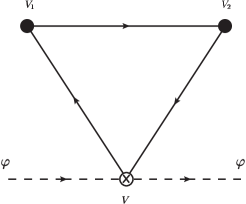
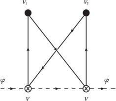
Figure 1: The mechanism of mediation of supersymmetry breaking from the hidden brane ( solid vertices on top ) to the visible brane ( crossed vertices at bottom ) via exchanges of fermions and gravitinos which are represented by solid lines. The dashed lines represent scalar particles living on the visible brane. A one-loop graph ( left pane ) and a two-loop graph ( right pane ), giving rise to a scalar mass, are displayed.

In figure 1 we give examples of mass corrections to the visible scalar fields. In this, lower vertices $\,V$ are on the visible brane and upper vertices $\,V_{1,2}\,$ are located on the hidden brane. The dashed lines represent scalar fields on the visible brane and the solid lines all possible fermion propagators that can be drawn. The vertices $\,V$, stemming from the interaction (36), give rise to soft scalar masses squared. Similar graphs with $\,V$ replaced by the interaction (37) induce trilinear soft couplings. Allowing for gauge fields on the brane gaugino masses can arise in a similar manner. In that case gaugino fields can be also exchanged ( see [32]). From the one-loop graph on the left pane of 1 we have a contribution which, suppressing all indices, for simplicity, is given by

$$m_{0}^{2}\,=\,\int\,d^{4}p\,Tr\,\left[\,V\,\Delta(p,0,\pi R)\,V_{1}\,\Delta(p,\pi R,\pi R)\,V_{2}\,\Delta(p,\pi R,0)\,\right]$$ (40)

External momenta of the scalar fields have been put to zero. The graph on the right pane has a similar structure. In (40) $\,\Delta$ denotes either a gravitino or a fermion propagators in all possible ways allowed by the interactions, and the mass terms are treated as insertions. For the graphs displayed in 1 the vertices are $\,V=k_{5}^{2}\,\mathchoice{\ooalign{$\hfil\displaystyle\mkern 0.0mu/\hfil$\crcr$\displaystyle p$}}{\ooalign{$\hfil\textstyle\mkern 0.0mu/\hfil$\crcr$\textstyle p$}}{\ooalign{$\hfil\scriptstyle\mkern 0.0mu/\hfil$\crcr$\scriptstyle p$}}{\ooalign{$\hfil\scriptscriptstyle\mkern 0.0mu/\hfil$\crcr$\scriptscriptstyle p$}}$ and $\,V_{1}=V_{2}=k_{5}^{2}\,c\,$ as follows from (36) and (37). Thus up to a dimensionless constant (40) yields

$$m_{0}^{2}\, = \,i\,k_{5}^{6}\,{|c|}^{2}\,\int\,\dfrac{d^{4}\,p}{{(2\pi)}^{4}}\,\dfrac{p^{4}\,cos(q\pi R)}{{(q\,sin(q\pi R))}^{3}}\,=\,k_{5}^{6}\,{|c|}^{2}\,\dfrac{2\pi^{2}}{{(2\pi)}^{4}}\,\int_{0}^{\infty}\,{d\,p_{E}\,p_{E}^{3}}\,\dfrac{p_{E}^{4}\,cosh(p_{E}\pi R)}{{(p_{E}\,sinh(p_{E}\pi R))}^{3}}$$ (41)

$$= k_{5}^{6}\,{|c|}^{2}\,\dfrac{1}{{(\pi R)}^{5}\,{(2\pi)}^{4}}\,\int_{0}^{\infty}\,{d\,\xi}\,\dfrac{\xi^{4}\,cosh\xi}{{\,sinh\xi}^{3}}\,=\,\dfrac{3\,\zeta(3)}{8}\,g\,m_{3/2}^{2}$$

In the first equation above $\,q\equiv\sqrt{-p^{2}}\,$ and in the second equation we passed to Euclidean momenta. Also the integration in the $\,\xi$ variable yields $\,3\,\zeta(3)$ where $\,\zeta(3)$ is the Riemann zeta function. In passing to the the last expression, we used the value of the lowest mode gravitino mass, $\,m_{3/2}\,=\,k_{5}^{2}\,c/\pi R\,$, and a dimensionless coupling was defined by $\,g\equiv\dfrac{k_{5}^{2}}{\pi^{2}\,V_{5}^{3}}\,$ with $\,V_{5}\,$ the volume of the compactifying manifold $\,V_{5}=\pi\,R$. Then the soft mass squared above is of the form

$$m_{0}^{2}\,=\,C_{1}\,g\,{m}^{2}_{3/2}$$ (42)

where $\,C_{1}\,$ is a finite non-zero dimensionless constant of order unity. The two loop graph on the right pane of 1 can be handled in the same way. In this case we have an extra vertex $\,V$ an extra fermion propagator and a scalar propagator on the visible brane. Its contribution is

$$m_{0,(2-loop)}^{2}\,=\hskip 341.43306pt$$

$$\,k_{5}^{8}\,{|c|}^{2}\,\int\,\dfrac{d\,p_{1}^{4}}{{(2\pi)}^{4}}\,\int\,\dfrac{d\,p_{2}^{4}}{{(2\pi)}^{4}}\,\dfrac{p_{1}^{\,2}}{{(q_{1}\,sin(q_{1}\pi R))}^{2}}\,\dfrac{p_{2}^{\,2}}{{(q_{2}\,sin(q_{2}\pi R))}^{2}}\,\dfrac{{(p_{1}+p_{2})}^{\,2}}{{(p_{1}-p_{2})}^{\,2}}$$ (43)

The momenta $q_{i}$ above are $\,q_{i}\equiv\sqrt{-p_{i}^{\,2}}$, see Eq. (39). Also $\,{(p_{1}+p_{2})}^{\,2}$ in the numerator comes from the two $V$-vertices while $\,{(p_{1}-p_{2})}^{\,2}$ in the denominator from the boson propagator on the visible brane. Notice that there are no $\,cosine$ terms in the numerator, as the ones appearing in (39), since all fermion propagators connect the visible to the hidden brane in this case. Certainly it is not our intention to proceed to a two loop calculation of the soft SUSY-breaking parameters and the only reason of presenting (43) is to derive an order of magnitude estimate that will be useful for the discussion that follows. Proceeding in the same way as before it is not hard to see, by first passing to Euclidean momenta and then rescaling them, in order to have dimensionless integrals, that a correction arises which is proportional to $\,\sim g^{\,2}\,{m}^{2}_{3/2}$. This argument is sufficient for one to be convinced that the dimensionless coupling $\,g$ defined before serves as a proper loop expansion parameter. This can be expressed in terms of the Planck mass as

$$g\,\equiv\,\dfrac{k_{5}^{2}}{\pi^{2}\,V_{5}^{3}}\,=\,\dfrac{1}{\pi^{3}\,R^{\,2}\,M_{Planck}^{\,2}}$$ (44)

Therefore from the previous discussion it is evident that the induced soft scalar masses can be written, in general, as

$$m_{0}^{2}\,=\,(\;\sum_{L}\,C_{L}\,g^{L}\;)\;{m}^{2}_{3/2}$$ (45)

Similar results hold for the soft gaugino masses and the trilinear couplings as well,

$$M_{1/2}\,=\,(\;\sum_{L}\,C_{L}\,g^{L}\;)\;{m}_{3/2}\quad,\quad A_{0}\,=\,(\;\sum_{L}\,C_{L}\,g^{L}\;)\;{m}_{3/2}$$ (46)

The constants $C_{k}$ are dimensionless and they are different, in general, for each of the parameters $\,m_{0}^{2},\,M_{1/2},\,A_{0}\,$. . It is obvious from these results that loop expansion is a valid approximation provided

$$g<1$$ (47)

or, on account of (44), when $\,R^{-1}<\pi^{3/2}\,M_{Planck}\,$ which allows for large values of the radius $\,R\,$.

It should be pointed out that, the corrections to the soft parameters presented before are valid to any loop order but only to lowest order in the gravitino mass. However, there are corrections that are of higher order in the gravitino mass. For instance, for the gaugino mass, if the quadratic in the gravitino mass corrections are added, we have

$$M_{1/2}\,=\,C_{1}\,g\,m_{3/2}\,(\,1\,+{\cal{O}}(1)\,\,R\,m_{3/2}\,)\,\;.$$ (48)

Therefore the calculation of the induced soft-supersymmetry breaking terms, to lowest order in the gravitino mass, can be trusted provided

$$R\,m_{3/2}<1$$ (49)

Thus in this approximation, given the value of $\,R$, an upper bound is imposed on the gravitino mass . In the regime (49), corrections that are of higher power in the gravitino mass are irrelevant. This facilitates calculations a great deal. Therefore we conclude that in addition to (47), which guarantees a valid perturbative expansion, the bound given by (49) should be observed so that the resulting soft breaking terms are trusted to lowest order approximation in the gravitino mass. Thus the region of the parameters for which the scheme presented makes sense is defined by (47) and (49) and these limits are important for phenomenological analysis

Using the bound (49) it is found that the induced gaugino mass $\,M_{1/2}\,\sim\,g\,m_{3/2}$ is also bounded from above by

$$M_{1/2}\,<\,g\,R^{\,-1}=\,\dfrac{R^{-3}}{\pi^{3}\;M_{Planck}^{2}}$$ (50)

while similar bounds hold for the other soft breaking parameters as well. The absence of any supersymmetry signals at LHC indicates that the upper bound (50) set for $\,M_{1/2}$ should be larger than a few $\;\mathrm{TeV}$, at least. Therefore (50) sets a lower bound on $\,R^{\,-1}$ which combined with the upper bound from (47) sets the allowed range of values for the size of the orbifold,

$$\pi\;M_{1/2}^{1/3}\;M_{Planck}^{2/3}\,<\,R^{-1}\,<\,\pi^{\,3/2}\,M_{Planck}$$ (51)

From this we derive a lower limit $\,R^{\,-1}\,\gtrsim 1.66\times 10^{\,11}\,$ TeV if $\,M_{1/2}\sim 1\,\text{TeV}$ . Therefore the radius $\,R$ can be large but not larger than $\,\sim\;10^{\,-11}\,{\mathrm{TeV}}^{-1}$, if supersymmetric masses are heavier than $\sim$ TeV. For a given value of $\,R$ in this regime the value of $\,g$ is determined by (44).

$\quad\quad\quad R^{\,-1}\quad\quad$	$\,\quad\quad g\quad\quad$	$\,m_{3/2}$	$M_{1/2},\,\,A_{\,0}\sim g\,m_{3/2}$	$m_{\,0}\sim\sqrt{g}\;m_{3/2}$
$10^{\,11}$ TeV	$10^{\,-10}$	$10^{\,10}\,-\,10^{\,11}$	$1\,-\,10$	$10^{\,5}\,-\,10^{\,6}$
$10^{\,14}$ TeV	$10^{\,-4}$	$10^{\,4}\,-\,10^{\,14}$	$1\,-\,10^{\,10}$	$10^{\,2}\,-\,10^{\,12}$
$10^{\,16}$ TeV	$1$	$1\,-\,10^{\,16}$	$1\,-\,10^{\,16}$	$1\,-\,10^{\,16}$

Table 1: In the first column the value of $\,R^{\,-1}$ is given ( in TeV ). In the second column the corresponding value of the loop expansion parameter $g$ is given and in the third the allowed range for the gravitino mass is shown. In the the fourth and fifth columns the corresponding allowed ranges for the soft SUSY-breaking parameters are given. All masses are in TeV .

The soft SUSY breaking parameters, and consequently the mass spectrum of supersymmetric particles, is determined when in addition to $R$ the value of the gravitino mass is given, which however should be smaller than $\,R^{\,-1}$ by (49). In Table 1 we display representative values of $\,R$, the corresponding values of $\,g$ and the allowed ranges for the gravitino mass and the soft breaking parameters. The lowest value of the gravitino mass is dictated by the fact that all supersymmetry breaking parameters are larger than one TeV. For the lowest allowed value of $\,R^{\,-1}$, displayed in this table, the parameter $\,g$ is tiny and the gravitino mass is constrained within rather narrow limits. Then the value of the gaugino mass is in the range of a few TeV. Note however that the soft mass $\,m_{0}$ is much larger. The reason is that the soft SUSY-breaking parameters have a different dependence on $\,g$. In particular $\,M_{1/2}$ and $\,A_{0}$ are linear in $\,g$ while $\,m_{0}$ is proportional to $\,\sqrt{g}$ and the soft masses are correlated having a ratio $\,M_{1/2}/m_{0}\sim\sqrt{g}\;$, which is independent of the gravitino mass. Thus smaller values of $g$ entail to larger masses for $\,m_{0}$ as compared to the gaugino masses. This forces $\,m_{0}$ to be considerably larger than $\,M_{1/2}$, for values of $\,R^{\,-1}$ in the range up to $\,10^{\,14}$ TeV. For higher $\,R^{\,-1}$ the soft mass $\,m_{0}$ is still larger than the other SUSY breaking parameters but not much. This is important for phenomenological studies since it shows that for small values of $\,R^{\,-1}$ the squarks and sleptons can be significantly heavier than the gauginos. This mimics the models of split supersymmetry [58, 59, 60, 61] and shows that in the proposed six-dimensional supergravity framework a split supersymmetry scenario can be accommodated, in principle.

As is seen from the last row of Table 1, as the value of $\,R^{\,-1}$ approaches the Planck scale the restrictions put on the gravitino mass, other than the phenomenological ones, are loosen and $\,m_{3/2}$ can take any value from the TeV to the Planck scale. In this case $g\simeq 1$ and the effective supersymmetry breaking scale in the observable sector is of the same order with the gravitino mass.

6 Conclusions

In this note, motivated by the recent developments pertinent to the six-dimensional description of the supergravity theory, we study the orbifolded $N=2$, $D=5$ supergravity as originating from a $D=6$ supergravity. In particular we considered a six-dimensional supergravity model, with tensor multiplets, which is truncated to a five-dimensional supergravity by the Kaluza - Klein approach, followed by orbifold compactification on $\,S_{1}/Z_{2}$. The arising model is described by a five-dimensional supergravity with two four-dimensional branes residing at the end points of $S_{1}/Z_{2}$, having local $N=1$ supersymmetry on them. The resulting model has striking similarities with supergravitiy models studied in the past that they are not connected to higher dimensional schemes. The novel features that the connection with the six-dimensional supergravity brings about, is the fact that additional chiral multiplets appear which can convey the messenge of supersymmetry breaking from one brane to the other. Besides, the particular compactification approach results to an effective supergravity on the four-dimensional branes with special characteristics. In particular the additional scalar fields, whose presence in due the tensor multiplets, parametrize a Kähler manifold having a no-scale structure which could not have been anticipated. The no-scale structure is dictated by the radion field, which is a combination of the moduli fields, and it is derived from the six-dimensional theory.

The supersymmetry breaking that takes place on the hidden brane is transmitted through the bulk by gravity to the observable fields which are assumed to be confined on one of the branes. The magnitude of the supersymmetry breaking is set by the gravitino mass and the size $R$ of the orbifold $\,S_{1}/Z_{2}$. The mechanism of supersymmetry breaking transmission reveals that finite soft supersymmetry breaking parameters are induced for the supersymmetric fields living on the visible brane. The perturbative mechanism of supersymmetry breaking can be trusted at one - loop approximation and to lowest order in the gravitino mass for values of $R^{\,-1}$ within a certain range which can be as large as the Planck scale but not smaller than $\sim 10^{\,11}\;\mathrm{TeV}$, if sparticles have to have masses larger than a few TeV as LHC experiments suggest. The gravitino mass is forced to lie within a narrow mass range, in the vicinity of $\,\sim 10^{\,10}\,\;\mathrm{TeV}$, for the lowest allowed value of $R^{\,-1}\sim 10^{\,11}\;\mathrm{TeV}$, but this range is broadened if $\,R^{\,-1}$ gets larger. The above scheme allows for sparticles to be considerably heavier than sfermions, when $R^{\,-1}\lesssim 10^{\,14}\;\mathrm{TeV}$, mimicking the models of split supersymmetry. For values of $R^{\,-1}$ approaching the Planck scale the gravitino mass and the corresponding SUSY breaking parameters are of the same order of magnitude and can take values in the whole range from a few TeV to $10^{\,16}$ TeV.

The salient qualitative features of the five-dimensional schemes regarding the supersymmetry breaking remain almost intact, indicating that the supersymmetry breaking mechanisms studied in the past can be easily incorporated in higher dimensional schemes. A more detailed theoretical and phenomenological study of these models will appear in a forthcoming publication.

Appendix

A The scalar potential on the brane

For the calculation of the scalar potential given in (27) we need $\,\mathcal{K}^{\alpha\beta^{*}}$ and $\,\mathcal{K}_{\alpha^{*}}$, as well as its complex conjugate $\,\mathcal{K}_{\alpha}$. The indices take values $i=0,1,2$, corresponding to the fields $a_{0},a_{1},a_{2}$, and $\,m$ corresponding to a scalar $\phi_{m}$ living on the branes. For $\,\mathcal{K}_{\alpha}$ we find from (26)

$$\mathcal{K}_{i}\,\; = \,-n_{i}\,(a_{i}+a_{i}^{*})^{-1}\,(\,1+\frac{1}{3}\,\Delta_{(5)}\,K\,)$$

$$\mathcal{K}_{m}\, = \,\Delta_{(5)}\,{K}_{m}$$ (A.1)

In these, $i=0,1,2$ and $\,n_{0}=2,n_{1}=n_{2}=1/2\,$ and $K$ is either $K_{V}$ or $K_{H}$ depending on which brane, visible or hidden, the scalar potential refers to ( see equation (26)). In the following we shall present the calculation for the scalar potential on the visible brane. The result can be applied for the hidden brane, as well, replacing the visible Kähler function and superpotential by the corresponding ones for the hidden brane. For definiteness in the following we shall assume that only one scalar field lives on the brane, $\varphi$. This suffices to demonstrate how one arrives at the result presented in (29). The elements of the inverse matrix $\,\mathcal{K}^{\alpha\beta^{*}}$ are given by

$$\mathcal{K}^{ji^{*}}\, = \,-n_{i}^{\,-1}\,\,(a_{i}+a_{i}^{*})^{2}\,\delta^{ji^{*}}\quad,\quad j,i^{*}=0,1,2$$

$$\mathcal{K}^{\varphi i^{*}}\, = \,(a_{i}+a_{i}^{*})\,\frac{K_{\varphi^{*}}}{3\,K_{\varphi\,\varphi^{*}}}\quad,\quad\mathcal{K}^{i\varphi^{*}}\,=\,(a_{i}+a_{i}^{*})\,\frac{K_{\varphi}}{3\,K_{\varphi\,\varphi^{*}}}$$

$$\mathcal{K}^{\varphi\varphi^{*}}\, = \frac{1}{\Delta_{(5)}}\,\frac{1}{K_{\varphi\,\varphi^{*}}}\,+\,\frac{K_{\varphi^{*}}\,K_{\varphi}}{3\,{K_{\varphi\,\varphi^{*}}^{2}}}$$ (A.2)

In deriving (A.2) we have omitted terms which are of order $\,\Delta_{(5)}$, or higher, the reason being that (27) already includes a prefactor $\,\Delta_{(5)}^{2}$ and we are interested in potential terms up to second order in $\,\Delta_{(5)}$.

For the calculation of the scalar potential we first write the expression in (27) which involves $\,\mathcal{K}^{\alpha\beta^{*}}$ as

$$\mathcal{K}^{\alpha\beta^{*}}\left[W_{\alpha}+\mathcal{K}_{\alpha}W\right]\left[\bar{W}_{\beta^{*}}+\mathcal{K}_{\beta^{*}}\bar{W}\right]$$

$$\quad\quad\quad\quad\,=\,\mathcal{K}_{\alpha}\mathcal{K}^{\alpha\beta^{*}}\mathcal{K}_{\beta^{*}}\,{|W|}^{2}\,+\,(\,\bar{W}\,W_{\varphi}\,\mathcal{K}^{\varphi\beta^{*}}\mathcal{K}_{\beta^{*}}\,+\,c.c\,)\,+\,\mathcal{K}^{\varphi\varphi^{*}}\,W_{\varphi}\,W_{\varphi^{*}}$$ (A.3)

In writing this we have made use of the fact that the superpotential $W$ does not depend on the fields $\,a_{i}$, therefore $\,W_{i}=\bar{W}_{i^{*}}=0$. Then having the analytic forms of the quantities given by (A.1) and (A.2) is fairly easy to see that

$$\mathcal{K}_{\alpha}\mathcal{K}^{\alpha\beta^{*}}\mathcal{K}_{\beta^{*}}\,=\,3\,+\,...$$ (A.4)

In it the ellipsis denote terms of order $\,\Delta_{(5)}$, which can be neglected if we keep terms in the potential that are most quadratic in $\,\Delta_{(5)}$. Recall that the potential, as given by equation (27), already carries a prefactor which is quadratic in $\,\Delta_{(5)}$. The result (A.4) states that the last negative term in the potential (27), namely $\,-3\,{|W|}^{2}$, is exactly cancelled by the first term appearing on the r.h.s. of (A.3). The terms in (A.3) which involve $\,\mathcal{K}^{\varphi\beta^{*}}\mathcal{K}_{\beta^{*}}$ are easily found to be proportional to $\,\Delta_{(5)}$ and hence do not contribute to the desired order. Therefore it only remains to examine the last term $\,\mathcal{K}^{\varphi\varphi^{*}}\,W_{\varphi}\,W_{\varphi^{*}}$, which by using the expression for $\,\mathcal{K}^{\varphi\varphi^{*}}$ in (A.2), yields

$$\mathcal{K}^{\varphi\varphi^{*}}\,W_{\varphi}\,W_{\varphi^{*}}\, = \,\left(\frac{1}{\Delta_{(5)}}\,\frac{1}{K_{\varphi\,\varphi^{*}}}\,+\,\frac{K_{\varphi}^{*}\,K_{\varphi}}{3\,{K_{\varphi\,\varphi^{*}}^{2}}}\,\right)\,W_{\varphi}\,W_{\varphi^{*}}$$

$$= \,\frac{1}{\Delta_{(5)}}\,{K^{\varphi\,\varphi^{*}}}\,W_{\varphi}\,W_{\varphi^{*}}\,\left(\,1+\frac{\Delta_{(5)}}{3}\,{K^{\varphi\,\varphi^{*}}}\mathcal{K}_{\varphi}\,\mathcal{K}_{\varphi^{*}}\right)$$ (A.5)

In passing to the last equation we used the fact $\,{K^{\varphi\,\varphi^{*}}}\,{K_{\varphi\,\varphi^{*}}}=1$. Using the above equation in (27) we arrive at

$$V_{scalar}\,=\,\Delta_{(5)}\,e^{\mathcal{K}}K^{\varphi\varphi^{*}}W_{\varphi}\bar{W}_{\varphi^{*}}\,\left(\,1\,+\,\frac{1}{3}\,\Delta_{(5)}\,K^{\varphi\varphi^{*}}K_{\varphi}\bar{K}_{\varphi^{*}}\,+\,\cdots\right)$$ (A.6)

which is just the result presented in equation (29) for the case of one chiral multiplet. This result can be generalized for an arbitrary number of multiplets and it can be also used for the hidden brane as well, with $K$ and $W$ replaced by their corresponding quantities on the hidden brane. Since we have assumed a constant superpotential on the hidden brane the derivatives $\,W_{\varphi}\,,\,\bar{W}_{\varphi^{*}}$ are set to zero yielding a vanishing scalar potential on the hidden brane.

References

-
[1]
C. Vafa,
“Evidence for F theory,” Nucl. Phys. B 469, 403 (1996) [hep-th/9602022].
D. R. Morrison and C. Vafa, “Compactifications of F theory on Calabi-Yau threefolds. 1,” Nucl. Phys. B 473, 74 (1996) [hep-th/9602114].
D. R. Morrison and C. Vafa, “Compactifications of F theory on Calabi-Yau threefolds. 2.,” Nucl. Phys. B 476, 437 (1996) [hep-th/9603161]. - [2] P. Horava and E. Witten, Nucl. Phys. B 460 (1996) 506 [arXiv:hep-th/9510209]; P. Horava and E. Witten, Nucl. Phys. B 475 (1996) 94 [arXiv:hep-th/9603142]; E. Witten, Nucl. Phys. B 471 (1996) 135 [arXiv:hep-th/9602070].
- [3] A. Lukas, B. A. Ovrut, K. S. Stelle and D. Waldram, “Heterotic M-theory in five dimensions,” Nucl. Phys. B 552 (1999) 246 [arXiv:hep-th/9806051];
- [4] S. Mizoguchi and N. Ohta, “More on the similarity between D = 5 simple supergravity and M theory,” Phys. Lett. B 441, 123 (1998) [arXiv:hep-th/9807111].
- [5] S. Ferrara, R. Minasian and A. Sagnotti, “Low-energy analysis of M and F theories on Calabi-Yau threefolds,” Nucl. Phys. B 474, 323 (1996) [hep-th/9604097].
- [6] F. Bonetti and T. W. Grimm, “Six-dimensional (1,0) effective action of F-theory via M-theory on Calabi-Yau threefolds,” JHEP 1205, 019 (2012) [arXiv:1112.1082 [hep-th]].
- [7] F. Bonetti, T. W. Grimm and S. Hohenegger, “Exploring 6D origins of 5D supergravities with Chern-Simons terms,” JHEP 1305, 124 (2013) [arXiv:1303.2661 [hep-th]].
- [8] A. Lukas, B. A. Ovrut, K. S. Stelle and D. Waldram, “The universe as a domain wall,” Phys. Rev. D 59 (1999) 086001 [arXiv:hep-th/9803235];
- [9] For a review see R. Maartens and K. Koyama, “Brane-World Gravity,” Living Rev. Rel. 13, 5 (2010) [arXiv:1004.3962 [hep-th]].
- [10] S. Choudhury and S. Pal, “Brane inflation in background supergravity,” Phys. Rev. D 85, 043529 (2012) [arXiv:1102.4206 [hep-th]].
-
[11]
For a review see D. J. H. Chung, L. L. Everett, G. L. Kane, S. F. King, J. D. Lykken and L. T. Wang,
“The soft supersymmetry-breaking Lagrangian: Theory and applications,”
Phys. Rept. 407, 1 (2005)
[arXiv:hep-ph/0312378].
Z. Kakushadze and S. H. H. Tye, “Brane world,” Nucl. Phys. B 548 (1999) 180 [arXiv:hep-th/9809147]. -
[12]
A. H. Chamseddine, R. Arnowitt and P. Nath,
“Locally Supersymmetric Grand Unification,”
Phys. Rev. Lett. 49 (1982) 970, 11;
L. J. Hall, J. D. Lykken and S. Weinberg, “Supergravity As The Messenger Of Supersymmetry Breaking,” Phys. Rev. D 27 (1983) 2359;
N. Ohta, “Grand Unified Theories Based On Local Supersymmetry,” Prog. Theor. Phys. 70 (1983) 542. - [13] I. Antoniadis, C. Munoz and M. Quiros, “Dynamical supersymmetry breaking with a large internal dimension,” Nucl. Phys. B 397 (1993) 515 [arXiv:hep-ph/9211309]; N. Arkani-Hamed, S. Dimopoulos and G. R. Dvali, “The hierarchy problem and new dimensions at a millimeter,” Phys. Lett. B 429 (1998) 263 [arXiv:hep-ph/9803315]; I. Antoniadis, N. Arkani-Hamed, S. Dimopoulos and G. R. Dvali, “New dimensions at a millimeter to a Fermi and superstrings at a TeV,” Phys. Lett. B 436 (1998) 257 [arXiv:hep-ph/9804398].
- [14] E. A. Mirabelli and M. E. Peskin, “Transmission of supersymmetry breaking from a 4-dimensional boundary,” Phys. Rev. D 58 (1998) 065002 [arXiv:hep-th/9712214].
- [15] Z. Chacko, M. A. Luty, I. Maksymyk and E. Ponton, “Realistic anomaly-mediated supersymmetry breaking,” JHEP 0004 (2000) 001 [arXiv:hep-ph/9905390].
- [16] I. Jack and D. R. T. Jones, “R-symmetry, Yukawa textures and anomaly mediated supersymmetry breaking,” Phys. Lett. B 491 (2000) 151 [arXiv:hep-ph/0006116].
-
[17]
J. A. Bagger, F. Feruglio and F. Zwirner,
“Generalized symmetry breaking on orbifolds,”
Phys. Rev. Lett. 88, 101601 (2002)
[arXiv:hep-th/0107128];
J. Bagger, F. Feruglio and F. Zwirner, “Brane induced supersymmetry breaking,” JHEP 0202, 010 (2002) [arXiv:hep-th/0108010]. - [18] H. P. Nilles, M. Olechowski and M. Yamaguchi, “Supersymmetry breakdown at a hidden wall,” Nucl. Phys. B 530, 43 (1998) [arXiv:hep-th/9801030].
- [19] A. Falkowski, Z. Lalak and S. Pokorski, “Supersymmetrizing branes with bulk in five-dimensional supergravity,” Phys. Lett. B 491 (2000) 172 [arXiv:hep-th/0004093].
-
[20]
Z. Chacko and M. A. Luty,
“Radion mediated supersymmetry breaking,”
JHEP 0105 (2001) 067
[arXiv:hep-ph/0008103];
D. E. Kaplan and N. Weiner, “Radion mediated supersymmetry breaking as a Scherk-Schwarz theory,” arXiv:hep-ph/0108001. - [21] K. A. Meissner, H. P. Nilles and M. Olechowski, “Brane induced supersymmetry breakdown and restoration,” Acta Phys. Polon. B 33, 2435 (2002) [arXiv:hep-th/0205166];
- [22] M. A. Luty and N. Okada, “Almost no-scale supergravity,” JHEP 0304 (2003) 050 [arXiv:hep-th/0209178].
- [23] I. L. Buchbinder, S. J. J. Gates, H. S. J. Goh, W. D. I. Linch, M. A. Luty, S. P. Ng and J. Phillips, “Supergravity loop contributions to brane world supersymmetry breaking,” Phys. Rev. D 70 (2004) 025008 [arXiv:hep-th/0305169].
- [24] T. Gherghetta and A. Riotto, “Gravity-mediated supersymmetry breaking in the brane-world,” Nucl. Phys. B 623, 97 (2002) [arXiv:hep-th/0110022].
- [25] R. Rattazzi, C. A. Scrucca and A. Strumia, “Brane to brane gravity mediation of supersymmetry breaking,” Nucl. Phys. B 674, 171 (2003) [arXiv:hep-th/0305184].
- [26] C. A. Scrucca, “Mediation of supersymmetry breaking in extra dimensions,” Mod. Phys. Lett. A 20, 297 (2005) [arXiv:hep-th/0412237].
- [27] T. Gregoire, R. Rattazzi and C. A. Scrucca, “D-type supersymmetry breaking and brane-to-brane gravity mediation,” Phys. Lett. B 624, 260 (2005) [arXiv:hep-ph/0505126].
- [28] T. Gregoire, R. Rattazzi, C. A. Scrucca, A. Strumia and E. Trincherini, “Gravitational quantum corrections in warped supersymmetric brane worlds,” Nucl. Phys. B 720, 3 (2005) [arXiv:hep-th/0411216].
- [29] K. Schmidt-Hoberg, “Supersymmetry breaking in five and six space-time dimensions,” DESY-THESIS-2005-009.
- [30] G. A. Diamandis, B. C. Georgalas, P. Kouroumalou and A. B. Lahanas, “On the brane coupling of unified orbifolds with gauge interactions in the bulk,” Phys. Lett. B 602, 112 (2004) [arXiv:hep-th/0402228].
- [31] G. A. Diamandis, B. C. Georgalas, P. Kouroumalou and A. B. Lahanas, “On the radion mediation of the Supersymmetry breaking in N=2, D=5 Supergravity Orbifolds,” Phys. Lett. B 660 (2008) 247 [arXiv:0711.1414 [hep-th]].
- [32] G. A. Diamandis, B. C. Georgalas, P. Kouroumalou and A. B. Lahanas, “The soft supersymmetry breaking in D=5 supergravity compactified on orbifolds,” Phys. Lett. B 692, 26 (2010) [arXiv:1001.5382 [hep-th]].
- [33] M. McGarrie and R. Russo, “General Gauge Mediation in 5D,” Phys. Rev. D 82, 035001 (2010) [arXiv:1004.3305 [hep-ph]].
- [34] M. McGarrie and D. C. Thompson, “Warped General Gauge Mediation,” Phys. Rev. D 82, 125034 (2010) [arXiv:1009.4696 [hep-th]].
- [35] C. Bouchart, A. Knochel and G. Moreau, “Discriminating 4D supersymmetry from its 5D warped version,” Phys. Rev. D 84, 015016 (2011) [arXiv:1101.0634 [hep-ph]].
- [36] H. Nishino and E. Sezgin, “Matter and Gauge Couplings of N=2 Supergravity in Six-Dimensions,” Phys. Lett. B 144, 187 (1984).
- [37] L. J. Romans, “Selfduality for Interacting Fields: Covariant Field Equations for Six-dimensional Chiral Supergravities,” Nucl. Phys. B 276, 71 (1986).
- [38] H. Nishino and E. Sezgin, “The Complete , Supergravity With Matter and Yang-Mills Couplings,” Nucl. Phys. B 278, 353 (1986).
- [39] J. H. Schwarz, “Anomaly - free supersymmetric models in six-dimensions,” Phys. Lett. B 371, 223 (1996) [hep-th/9512053].
- [40] N. Seiberg and E. Witten, “Comments on string dynamics in six-dimensions,” Nucl. Phys. B 471, 121 (1996) [hep-th/9603003].
- [41] H. Nishino and E. Sezgin, “New couplings of six-dimensional supergravity,” Nucl. Phys. B 505, 497 (1997) [hep-th/9703075].
- [42] S. Ferrara, F. Riccioni and A. Sagnotti, “Tensor and vector multiplets in six-dimensional supergravity,” Nucl. Phys. B 519, 115 (1998) [hep-th/9711059].
- [43] F. Riccioni, “All couplings of minimal six-dimensional supergravity,” Nucl. Phys. B 605, 245 (2001) [hep-th/0101074].
- [44] S. D. Avramis, A. Kehagias and S. Randjbar-Daemi, “A New anomaly-free gauged supergravity in six dimensions,” JHEP 0505, 057 (2005) [hep-th/0504033].
- [45] S. D. Avramis and A. Kehagias, “A Systematic search for anomaly-free supergravities in six dimensions,” JHEP 0510, 052 (2005) [hep-th/0508172].
- [46] P. Kouroumalou, talk given at ”Miami 2013”, Lago Mar Resort, Florida, 12 - 18 December, 2013 .
-
[47]
B. de Wit and H. Nicolai,
“N=8 Supergravity,”
Nucl. Phys. B 208, 323 (1982);
M. Pernici, K. Pilch and P. van Nieuwenhuizen,
“Gauged Maximally Extended Supergravity In Seven-Dimensions,”
Phys. Lett. B 143, 103 (1984);
“Gauged N=8 D=5 Supergravity,”
Nucl. Phys. B 259, 460 (1985),
M. Gunaydin, G. Sierra and P. K. Townsend, “The Geometry Of N=2 Maxwell-Einstein Supergravity And Jordan Algebras,” Nucl. Phys. B 242 (1984) 244 ; “Exceptional Supergravity Theories And The Magic Square,” Phys. Lett. B 133 (1983) 72; “More On D = 5 Maxwell-Einstein Supergravity: Symmetric Spaces And Kinks,” Class. Quant. Grav. 3 (1986) 763; “Quantization Of The Gauge Coupling Constant In A Five-Dimensional Yang-Mills / Einstein Supergravity Theory,” Phys. Rev. Lett. 53 (1984) 322; M. Gunaydin, G. Sierra and P. K. Townsend, “Vanishing Potentials In Gauged N=2 Supergravity: An Application Of Jordan Algebras,” Phys. Lett. B 144 (1984) 41,
B. de Wit and A. Van Proeyen, “Special geometry, cubic polynomials and homogeneous quaternionic spaces,” Commun. Math. Phys. 149, 307 (1992) [arXiv:hep-th/9112027]. - [48] M. Gunaydin and M. Zagermann, “The gauging of five-dimensional, N = 2 Maxwell-Einstein supergravity theories coupled to tensor multiplets,” Nucl. Phys. B 572 (2000) 131 [arXiv:hep-th/9912027]; M. Gunaydin and M. Zagermann, “The vacua of 5d, N = 2 gauged Yang-Mills/Einstein/tensor supergravity: Abelian case,” Phys. Rev. D 62 (2000) 044028 [arXiv:hep-th/0002228]. J. R. Ellis, Z. Lalak, S. Pokorski and S. Thomas, “Supergravity and supersymmetry breaking in four and five dimensions,” Nucl. Phys. B 563 (1999) 107 [arXiv:hep-th/9906148]; A. Falkowski, Z. Lalak and S. Pokorski, “Five-dimensional gauged supergravities with universal hypermultiplet and warped brane worlds,” Phys. Lett. B 509 (2001) 337 [arXiv:hep-th/0009167]; E. Bergshoeff, R. Kallosh and A. Van Proeyen, “Supersymmetry in singular spaces,” JHEP 0010 (2000) 033 [arXiv:hep-th/0007044].
- [49] E. Cremmer, S. Ferrara, C. Kounnas and D. V. Nanopoulos, “Naturally Vanishing Cosmological Constant In N=1 Supergravity,” Phys. Lett. B 133 (1983) 61; J. R. Ellis, A. B. Lahanas, D. V. Nanopoulos and K. Tamvakis, “No-Scale Supersymmetric Standard Model,” Phys. Lett. B 134, 429 (1984).
- [50] P. Van Nieuwenhuizen, “Supergravity,” Phys. Rept. 68, 189 (1981).
- [51] J. A. Bagger and D. V. Belyaev, “Brane-localized Goldstone fermions in bulk supergravity,” Phys. Rev. D 72 (2005) 065007 [arXiv:hep-th/0406126].
- [52] K. Benakli and C. Moura, “Brane-Worlds Pseudo-Goldstinos,” arXiv:0706.3127 [hep-th].
- [53] A. Falkowski, H. M. Lee and C. Ludeling, “Gravity mediated supersymmetry breaking in six dimensions,” JHEP 0510, 090 (2005) [hep-th/0504091].
- [54] Y. Sakamura and Y. Yamada, “Impacts of non-geometric moduli on effective theory of 5D supergravity,” JHEP 1311, 090 (2013) [arXiv:1307.5585 [hep-th]].
- [55] S. L. Parameswaran and J. Schmidt, “Coupling Brane Fields to Bulk Supergravity,” Phys. Lett. B 696, 131 (2011) [arXiv:1008.3832 [hep-th]].
- [56] N. Arkani-Hamed, L. J. Hall, Y. Nomura, D. R. Smith and N. Weiner, “Finite radiative electroweak symmetry breaking from the bulk,” Nucl. Phys. B 605 (2001) 81 [arXiv:hep-ph/0102090].
- [57] M. Puchwein and Z. Kunszt, “Radiative corrections with 5D mixed position- / momentum-space propagators,” Annals Phys. 311, 288 (2004) [arXiv:hep-th/0309069].
- [58] G. F. Giudice and A. Romanino, “Split supersymmetry,” Nucl. Phys. B 699 (2004) 65 [Erratum-ibid. B 706 (2005) 65] [hep-ph/0406088].
- [59] J. D. Wells, “Implications of supersymmetry breaking with a little hierarchy between gauginos and scalars,” hep-ph/0306127.
- [60] N. Arkani-Hamed and S. Dimopoulos, “Supersymmetric unification without low energy supersymmetry and signatures for fine-tuning at the LHC,” JHEP 0506 (2005) 073 [hep-th/0405159] ; N. Arkani-Hamed, S. Dimopoulos, G. F. Giudice and A. Romanino, ‘Aspects of split supersymmetry,” Nucl. Phys. B 709 (2005) 3 [hep-ph/0409232].
- [61] I. Antoniadis and S. Dimopoulos, “Splitting supersymmetry in string theory,” Nucl. Phys. B 715 (2005) 120 [hep-th/0411032].