Abstract

We present a non-minimal renormalizable SUSY $SU(5)$ model, with extended Higgs sector and right-handed neutrinos, where the flavour sector exhibits a $Q_{6}$ flavour symmetry. We analysed the simplest version of this model, in which R-parity is conserved and the right-handed neutrino masses in the flavour doublet are considered with and without degeneration. We find the generic form of the mass matrices both in the quark and lepton sectors. We reproduce, according to current data, the mixing in the CKM matrix. In the leptonic sector, in the general case where the right-handed neutrino masses are not degenerate, we find that the values for the solar, atmospheric, and reactor mixing angles are in very good agreement with the experimental data, both for a normal and an inverted hierarchy. In the particular case where the right handed neutrinos masses are degenerate, the model predicts a strong inverted hierarchy spectrum and a sum rule among the neutrino masses. In this case the atmospheric and solar angles are in very good agreement with experimental data, and the reactor one is different from zero, albeit too small ($\theta^{\ell^{th}}_{13}\sim 3.38^{\circ}$). This value constitues a lower bound for $\theta_{13}$ in the general case. We also find the range of values for the neutrino masses in each case.

1 Introduction

Understanding the flavour sector of the Standard Model (SM) has been a puzzle for a long time, due to the large differences in the Yukawa couplings of the different fermions. The hierarchy between the fundamental particles, the amount of CP violation and the structure of the CKM matrix remains as open [1]. In spite of these subtle facts, the success of the SM is remarkable.

One of the strategies to deal with the flavour problem in the quark and lepton sectors has been to study it in the framework of textures (zeros) in the mass matrices. The textures have been explored for a long time, as an attempt to eliminate the irrelevant free parameters in the Yukawa sector. As it is well known, the Fritzsch textures can accommodate the quarks mixing angles, in terms of the quarks masses [2, 3]. This approach seems to work out correctly because the Cabbibo angle is obtained with great accuracy [2]. However, this framework presents some problems with the top mass and the $V_{cb}$ element of the CKM matrix [4, 5], as can be seen in [6, 7]. Recently, deviations to the Fritzsch textures have appeared in order to overcome these problems. Moreover, the charged lepton and neutrino sector have been included in this kind of ansatz and consistent results on the PMNS matrix [8, 9] have been observed in this generic approximation [7]. As alternative textures to the Fritzsch ones, the Nearest Neighbour Interaction (NNI) textures can also reproduce very well the flavour mixing in the quark and lepton sectors [10, 11]; it is well known that Fritzsch textures could be obtained from the NNI ones as a limiting case [10].

Non-Abelian flavour symmetries have been playing an important role in model building, these symmetries are considered as an elegant way to obtain the NNI textures in the fermion mass matrices [11, 10]. In particular, the flavour symmetry group $Q_{6}$ [12] has been proposed as responsible of these kind of textures in the quarks as well as in the leptonic sector [13, 14, 15, 16, 17]. The rich phenomenology that $Q_{6}$ provides in the SUSY scenario is remarkable, one of these features is to prohibit the dangerous terms that mediate fast proton decay, rather than invoking the $R$-parity symmetry [14, 15]. The immediate question that arises is, how does the $Q_{6}$ symmetry work within a GUT framework? In particular, the main question that we will address here is if the SUSY-$SU(5)$ models are compatible with the $Q_{6}$ group in order to accommodate masses and mixings for fermions.

From a theoretical point of view, Grand Unified ideas are well motivated for fundamental reasons [18, 19, 20, 21]. In particular, the $SU(5)$ model [21] is considered to be one of the best scenarios to unify the electroweak and strong interactions. However, the model itself faces serious phenomenological and theoretical problems, one of them being that active neutrinos are massless [22, 23]; another one that the unification of gauge couplings is not quite good with the current precision data. The simplicity of the $SU(5)$ can be retained even if it is promoted to be a supersymmetric model. The SUSY $SU(5)$ [24, 25, 26] version, with $R$-parity conserved, gives a much better unification of the gauge couplings, but new couplings (five dimensional operators [27, 28]) can yield the proton decay [29, 30, 31], and therefore, they can exclude the SUSY version [32, 33, 34]. On the other hand, generic studies on the minimal SUSY $SU(5)$ model have made clear that it may not be ruled out by the experimental data on the proton decay rates [35, 36, 37]. Taking into account the neutrino mass problem, the SUSY $SU(5)$ version (SUSY models in general) provides elegant mechanisms to generate massive neutrinos via $R$-parity violation [38, 39]. But still, the simplest way to give mass to the left-handed neutrinos in the minimal $SU(5)$ or SUSY scenario is to consider three right-handed neutrinos (RHN’s) which are singlets under the gauge group and invoke the type I see-saw mechanism [40, 41, 42, 43, 44].

There are interesting SUSY $SU(5)$ models [45, 46, 47], that can very well reproduce the CKM and PMNS matrices in agreement with the experimental results, but where the simplicity in the matter content has been left aside. Most of these models include a large number of flavons which are required to accommodate correctly the mixings. A different approach consists of extending the Higgs sector of the models. By itself, the SUSY $SU(5)$ matter content provides the tools to accommodate masses and mixings via the extension of the Higgs scalar sector, although gauge coupling unification may be compromised. This philosophy has been worked out with success in non-supersymmetric [48, 49, 50] and supersymmetric [13, 14, 15, 16, 17] scenarios where the concept of flavour has been extended to the Higgs sector.

Therefore, we propose here a renormalizable SUSY $SU(5)$ model where the $Q_{6}$ group plays an important role in the flavour sector. The need to extend the scalar sector is evident in order to accommodate masses and mixings for quarks and leptons without breaking explicitly the flavour symmetry, so that three families of $H^{u}$ and $H^{d}$ $5$-plets are introduced. At the same time, three RHN’s are included by hand, and the type I see-saw mechanism is invoked to get small masses for the active neutrinos. At low energies when the first and second RHN masses are degenerate, a lower bound for the reactor angle, $\theta_{13}^{\ell}$, is obtained. Namely, consistent results are obtained for the CKM matrix in the quark sector, while in the leptonic sector, the values obtained for atmospheric and solar mixing angles are; $\theta^{\ell^{th}}_{23}=\left(46.18^{+0.66}_{-0.65}\right)^{\circ}$ and $\theta^{\ell^{th}}_{12}=\left(36.62\pm 4.06\right)^{\circ}$, which are consistent with experimental data. However, the reactor mixing angle value $\theta^{\ell^{th}}_{13}=\left(3.38^{+0.03}_{-0.02}\right)^{\circ}$, is not in good agreement with the central values of the global fits but it is still within the error bar of the different experiments, and fairly large in comparison to the tribimaximal scenario. This value corresponds to a lower bound for the reactor mixing angle of the more general case where the RHN’s are not mass degenerate, similar to the case of $S_{3}$ non-supersymmetric models, where relaxing the degeneracy condition in the RHN masses gives the right value for $\theta_{13}^{\ell}$ [50]. So, in order to enhance the theoretical value of the reactor mixing angle, which must be in accordance with the current experimental data, we consider that the two first RHN’s, $N_{1}$ and $N_{2}$, have different masses in the Majorana mass term. This assumption allows to get the following values for the normal [inverted] hierarchy: $\theta_{12}^{\ell^{th}}=\left(34.71_{-0.98}^{+0.91}\right)^{\circ}$ $\left[\left(34.73_{-1.11}^{+0.89}\right)^{\circ}\right]$, $\theta_{23}^{\ell^{th}}=\left(45.83_{-3.98}^{+4.49}\right)^{\circ}$ $\left[\left(48.57_{-2.76}^{+2.07}\right)^{\circ}\right]$, and $\theta_{13}^{\ell^{th}}=\left(8.77_{-0.32}^{+0.40}\right)^{\circ}$ $\left[\left(8.93_{-0.39}^{+0.33}\right)^{\circ}\right]$.

The paper is organized as follows: In section 2, we build the extended SUSY $SU(5)$ model which obeys the $Q_{6}$ flavour symmetry, in addition, we explain the required matter content to get a unified scenario and we do stress the strong assumptions that we will make in the model; at the same time, the ansatz to increase the value of reactor mixing angle is discussed. The textures in the quark mass matrices, and therefore their consequences in the lepton sector, are analysed in section 3. Also, we describe how to diagonalize the mass matrices for each sector, with particular attention to neutrino sector. In section 4, we present and discuss the results about the mixing angles for each sector. Finally, we give conclusions on this preliminary analysis of the model.

2 SUSY $SU(5)\otimes Q_{6}$ model

We will consider the SUSY $SU(5)$ model where three right-handed neutrinos have been included in the matter content. In addition, the scalar sector has to be necessarily extended as we will show. Thus, the matter content that will be used in the present model is displayed on Table 1, where the assignments under $Q_{6}$ flavour symmetry are shown.

	$SU(5)$	$Q_{6}$
$\left(H^{d}_{1},H^{d}_{2}\right)$	${\bf\bar{5}}$	${\bf 2}_{1}$
$H^{d}_{3}$	${\bf\bar{5}}$	${\bf 1}_{+,2}$
$\left(H^{u}_{1},H^{u}_{2}\right)$	${\bf 5}$	${\bf 2}_{1}$
$H^{u}_{3}$	${\bf 5}$	${\bf 1}_{+,2}$
$\left(F_{1},F_{2}\right)$	${\bf\bar{5}}$	${\bf 2}_{2}$
$F_{3}$	${\bf\bar{5}}$	${\bf 1}_{-,3}$
$\left(T_{1},T_{2}\right)$	${\bf 10}$	${\bf 2}_{2}$
$T_{3}$	${\bf 10}$	${\bf 1}_{-,3}$
$\left(N^{c}_{1},N^{c}_{2}\right)$	${\bf 1}$	${\bf 2}_{2}$
$N^{c}_{3}$	${\bf 1}$	${\bf 1}_{-,1}$
$Y_{B}$	${\bf 1}$	${\bf 1}_{+,2}$
$H_{\bar{45}}$	${\bf\bar{45}}$	${\bf 1}_{+,2}$
$H_{45}$	${\bf 45}$	${\bf 1}_{+,2}$
$\Phi$	${\bf 24}$	${\bf 1}_{+,0}$

Table 1: Matter content in the SUSY $SU(5)\otimes Q_{6}$ model.

Let us comment on our notation and the matter content: $\Phi^{a}_{b}$ stands for the ${\bf 24}$ adjoint scalar representation which breaks ($\left\langle\Phi\right\rangle=\sigma\textrm{diag}\left(1,1,1,-3/2,-3/2\right)$) the SUSY $SU(5)$ gauge group to the MSSM; there are three families of Higgs type $H^{u}_{i}$ and $H^{d}_{j}$. Here, we ought to stress a point. Because we have extended the Higgs sector, gauge coupling unification is not guaranteed, since the Renormalization Group Equations (RGE) depend strongly on the number of Higgs families [51, 52]. This is a drawback in the present model, and it is the price we have to pay for going beyond the minimal SUSY $SU(5)$ model. A proper analysis of the RGE evolution, including also the right handed-neutrinos will be left for a future work. On the other hand, we do need to include $H_{45}$ and ${H}_{\bar{45}}$ scalar representations so as to fix the incorrect relation ${\bf M}_{d}={\bf M}^{T}_{e}$, although there are other ways to achieve it, see [53, 54]. In addition, there is flavon, $Y_{B}$, which has already been used in supersymmetric models [13, 14, 15, 16, 17] in order to have a flavour invariant Majorana mass matrix. Regarding the fermion sector, $N_{i}$ denotes the RHN, which is a singlet under the $SU(5)$ gauge group; $F_{i}$ and $T_{j}$ stand for the ${\bf 5}$-plets and the ${\bf 10}$ antisymmetric-plet, respectively. Here, $a,b,c$ are $SU(5)$ indices, and $i,j$ are family indices. More explicitly,

$$F_{ia} = \left(d^{c},L\right);\quad T^{ab}_{j}=\dfrac{1}{\sqrt{2}}\left(u^{c},q,\ell^{c}\right);\quad L=\begin{pmatrix}\nu_{\ell}\\ \ell\end{pmatrix};\quad q=\begin{pmatrix}u\\ d\end{pmatrix},$$ (1)

$$H^{ua} = \begin{pmatrix}\texttt{H}^{u}\\ \textbf{H}^{u}\end{pmatrix};\quad H^{d}_{b}=\begin{pmatrix}\texttt{H}^{d}\\ \textbf{H}^{d}\end{pmatrix};\quad\textbf{H}^{u}=\begin{pmatrix}h^{+u}\\ h^{0u}\end{pmatrix};\quad\textbf{H}^{d}=\begin{pmatrix}h^{0d}\\ h^{-d}\end{pmatrix}.$$

Here, $\texttt{H}^{u}$ and $\texttt{H}^{d}$ are the coloured triplet scalars that mediate proton decay. For the time being, it will be assumed that these are heavy enough to keep proton lifetime bounded and under control. In addition, we have to point out that this subtle issue will be left aside, since we are only interested in studying the masses and mixings when implementing $Q_{6}$ as a flavour symmetry in this model. On the other hand, $\textbf{H}^{d}$ and $\textbf{H}^{u}$ are the weak doublets of the MSSM group. In consequence, we employ the following vacuum expectation values (vev’s) to get the fermion mass matrices.

$$\langle\textbf{H}^{u}\rangle = \begin{pmatrix}0\\ h^{0u}\end{pmatrix},\qquad\langle\textbf{H}^{d}\rangle=\begin{pmatrix}h^{0d}\\ 0\end{pmatrix},\qquad\left\langle H_{45}\right\rangle^{\alpha 5}_{\alpha}=v_{45},\qquad\left\langle H_{45}\right\rangle^{45}_{4}=-3v_{45}$$

$$\left\langle H_{\bar{45}}\right\rangle^{\alpha}_{\alpha 5} = v_{\bar{45}},\qquad\left\langle H_{\bar{45}}\right\rangle^{4}_{45}=-3v_{\bar{45}},\qquad\left\langle Y_{B}\right\rangle=v_{B}\qquad\alpha,\beta=1,2,3.$$ (2)

Having presented the assigned matter fields under the $Q_{6}$ flavour symmetry, we will now introduce the superpotential, gauge invariant under the $Q_{6}$ discrete group. All necessary details, on the multiplication rules of $Q_{6}$, are given in the appendix, where a brief review of this dihedral group is offered. The trilinear terms in the superpotential are given by

$$W =\sqrt{2}y^{d}_{1}\left(F_{1}T_{2}-F_{2}T_{1}\right)H^{d}_{3}+\sqrt{2}y^{d}_{2}\left(F_{1}T_{3}H^{d}_{2}-F_{2}T_{3}H^{d}_{1}\right)+\sqrt{2}y^{d}_{3}F_{3}\left(T_{1}H^{d}_{2}-T_{2}H^{d}_{1}\right)+\sqrt{2}y^{d}_{4}F_{3}T_{3}H^{d}_{3}$$

$$+\dfrac{y^{u}_{1}}{4}\left(T_{1}T_{2}-T_{2}T_{1}\right)H^{u}_{3}+\dfrac{y^{u}_{2}}{4}\left(T_{1}T_{3}H^{u}_{2}-T_{2}T_{3}H^{u}_{1}\right)+\dfrac{y^{u}_{3}}{4}T_{3}\left(T_{1}H^{u}_{2}-T_{2}H^{u}_{1}\right)+\dfrac{y^{u}_{4}}{4}T_{3}T_{3}H^{u}_{3}$$

$$+\sqrt{2}Y_{1}\left(F_{1}T_{2}-F_{2}T_{1}\right)H_{\bar{45}}+\sqrt{2}Y_{2}F_{3}T_{3}H_{\bar{45}}+\dfrac{\tilde{Y}_{1}}{4}\left(T_{1}T_{2}-T_{2}T_{1}\right)H_{45}+\dfrac{\tilde{Y}_{2}}{4}T_{3}T_{3}H_{45}$$

$$+y^{n}_{1}\left(N^{c}_{1}F_{2}-N^{c}_{2}F_{1}\right)H^{u}_{3}+y^{n}_{2}\left(N^{c}_{1}F_{3}H^{u}_{2}-N^{c}_{2}F_{3}H^{u}_{1}\right)+y^{n}_{3}N^{c}_{3}\left(F_{1}H^{u}_{2}+F_{2}H^{u}_{1}\right)+M_{R_{1}}\left(N^{c}_{1}N^{c}_{1}+N^{c}_{2}N^{c}_{2}\right)$$

$$+y^{m}_{2}N^{c}_{3}Y_{B}N^{c}_{3}.$$ (3)

It is important to remember that SUSY must be broken via soft breaking terms, so these soft breaking terms should be included in a complete study of the full scalar potential, but we do not include them in this preliminary analysis. The scalar superpotential is

$$W_{s} =\mu_{\Phi}Tr\left(\Phi^{2}\right)+\lambda_{\Phi}Tr\left(\Phi^{3}\right)+m_{45}H_{\bar{45}}H_{45}+\mu_{1}\left(H^{u}_{1}H^{d}_{2}-H^{u}_{2}H^{d}_{1}\right)+\mu_{2}H^{u}_{3}H^{d}_{3}$$

$$+\lambda_{1}\left(H^{u}_{1}\Phi H^{d}_{2}-H^{u}_{2}\Phi H^{d}_{1}\right)+\lambda_{2}H^{u}_{3}\Phi H^{d}_{3}+a_{1}H_{\bar{45}}H_{45}\Phi+a_{2}H_{\bar{45}}\Phi H^{u}_{3}+a_{3}H^{d}_{3}\Phi H_{45}.$$ (4)

From the superpotential given in Eq. (3), one must obtain the MSSM effective superpotential that contains the Yukawa mass term after spontaneous symmetry breaking via the vev’s of the $\textbf{H}^{u}$ and $\textbf{H}^{d}$ weak doublets scalar superfields. We will work in the following basis

$$\mathcal{L}=\mathcal{L}^{q}+\mathcal{L}^{l}$$ (5)

with

$$\begin{array}[]{l}\mathcal{L}^{q}=-\bar{d}_{iR}\left({\bf M}_{d}\right)_{ij}d_{jL}-\bar{u}_{iR}\left({\bf M}_{u}\right)_{ij}u_{jL}+h.c.\,,\\ \mathcal{L}^{l}=\bar{\ell}_{iR}\left({\bf M}_{\ell}\right)_{ij}\ell_{jL}-\bar{N}_{iR}\left({\bf M}_{D}\right)_{ij}\nu_{jL}-\frac{1}{2}\bar{N}_{iR}\left({\bf M}_{R}\right)_{ij}N^{c}_{jR}+h.c.\,,\end{array}$$ (6)

In general, the up, down, and charged lepton mass matrices are given by (see [55])

$${\bf M}_{u}=\dfrac{\left({\bf Y}^{u}+{\bf Y}^{uT}\right)}{2}\langle\textbf{H}^{u}\rangle-\left(\tilde{{\bf Y}}^{T}-\tilde{{\bf Y}}\right)v_{45},\quad{\bf M}_{d}={\bf Y}^{d}\langle\textbf{H}^{d}\rangle+2{\bf Y}v_{\bar{45}},\quad{\bf M}_{\ell}={\bf Y}^{dT}\langle\textbf{H}^{d}\rangle-6{\bf Y}^{T}v_{\bar{45}}.$$ (7)

In this particular model, from Eqs. (3) and (7) we have that the up, down and charged lepton mass matrices have respectively the following structures:

$${\bf M}_{u} =\begin{pmatrix}0&-2\tilde{Y}_{1}v_{45}&\bar{y}^{u}h^{0u}_{2}\\ 2\tilde{Y}_{1}v_{45}&0&-\bar{y}^{u}h^{0u}_{1}\\ \bar{y}^{u}h^{0u}_{2}&-\bar{y}^{u}h^{0u}_{1}&y^{u}_{4}h^{0u}_{3}\end{pmatrix},\,{\bf M}_{d}=\begin{pmatrix}0&y^{d}_{1}h^{0d}_{3}+2Y_{1}v_{\bar{45}}&y^{d}_{2}h^{0d}_{2}\\ -y^{d}_{1}h^{0d}_{3}-2Y_{1}v_{\bar{45}}&0&-y^{d}_{2}h^{0d}_{1}\\ y^{d}_{3}h^{0d}_{2}&-y^{d}_{3}h^{0d}_{1}&y^{d}_{4}h^{0d}_{3}+2Y_{2}v_{\bar{45}}\end{pmatrix};$$

$${\bf M}_{\ell} =\begin{pmatrix}0&-\left(y^{d}_{1}h^{0d}_{3}-6Y_{1}v_{\bar{45}}\right)&y^{d}_{3}h^{0d}_{2}\\ y^{d}_{1}h^{0d}_{3}-6Y_{1}v_{\bar{45}}&0&-y^{d}_{3}h^{0d}_{1}\\ y^{d}_{2}h^{0d}_{2}&-y^{d}_{2}h^{0d}_{1}&y^{d}_{4}h^{0d}_{3}-6Y_{2}v_{\bar{45}}\end{pmatrix}.$$ (8)

where $\bar{y}^{u}\equiv\left(y^{u}_{2}+y^{u}_{3}\right)/2$. As can be seen, the ${\bf M}_{u}$ mass matrix turns out almost symmetric due to the flavour structure. At the same time, we were able to correct the wrong relationship between the down quarks and the charged leptons; this was achieved including the $H_{\bar{45}}$ scalar representation. From Eq.(3), we obtain the Dirac (see Eq. (9)) and Majorana mass matrices, this latter is strictly given by ${\bf m}_{R}=\textrm{diag}\left(M_{R_{1}},M_{R_{1}},M_{R_{3}}=y^{m}_{2}v_{B}\right)$. We would like to mention at this point the ansatz to enhance the $\theta_{13}^{l}$ value, and its subtle ingredient, which consists in assuming that two RHN’s, $N_{1}$ and $N_{2}$, are not degenerated. Thus, the Majorana mass matrix is given in Eq. (9), and two cases will be studied later: $a)$ RHN’s degenerate, $b)$ RHN’s non-degenerate.

$${\bf M}_{D}=\begin{pmatrix}0&y^{n}_{1}h^{0u}_{3}&y^{n}_{2}h^{0u}_{2}\\ -y^{n}_{1}h^{0u}_{3}&0&-y^{n}_{2}h^{0u}_{1}\\ y^{n}_{3}h^{0u}_{2}&y^{n}_{3}h^{0u}_{1}&0\end{pmatrix}\quad\textrm{and}\quad{\bf M}_{R}=\begin{pmatrix}M_{R_{1}}&0&0\\ 0&M_{R_{2}}&0\\ 0&&M_{R_{3}}\end{pmatrix}.$$ (9)

Therefore, after the type I see-saw mechanism, the neutrino mass term is given by

$$\mathcal{L}_{\nu}=-\bar{N}_{iR}\left({\bf M}_{D}\right)_{ij}\nu_{jL}-\frac{1}{2}\bar{N}_{iR}\left({\bf M}_{R}\right)_{ij}N^{c}_{jR}+h.c.=-\frac{1}{2}\bar{\nu}^{C}_{L}{\bf M}_{\nu}\nu_{L}-\frac{1}{2}\bar{N}_{iR}\left({\bf M}_{R}\right)_{ij}N^{c}_{jR}.$$ (10)

where the ${\bf M}_{\nu}={\bf M}^{T}_{D}{\bf M}_{R}^{-1}{\bf M}_{D}$ effective neutrino mass matrix has the following structure:

$${\bf M}_{\nu}=\left(\begin{array}[]{ccc}\vspace{2mm}\frac{\left(y^{n}_{1}h^{0u}_{3}\right)^{2}}{M_{R_{2}}}+\frac{\left(y^{n}_{3}h^{0u}_{2}\right)^{2}}{M_{R_{3}}}&\frac{\left(y^{n}_{3}\right)^{2}h^{0u}_{2}h^{0u}_{1}}{M_{R_{3}}}&\frac{y^{n}_{1}h^{0u}_{3}y^{n}_{2}h^{0u}_{1}}{M_{R_{2}}}\\ \vspace{2mm}\frac{\left(y^{n}_{3}\right)^{2}h^{0u}_{2}h^{0u}_{1}}{M_{R_{3}}}&\frac{\left(y^{n}_{1}h^{0u}_{3}\right)^{2}}{M_{R_{1}}}+\frac{\left(y^{n}_{3}h^{0u}_{1}\right)^{2}}{M_{R_{3}}}&\frac{y^{n}_{1}h^{0u}_{3}y^{n}_{2}h^{0u}_{2}}{M_{R_{1}}}\\ \vspace{2mm}\frac{y^{n}_{1}h^{0u}_{3}y^{n}_{2}h^{0u}_{1}}{M_{R_{2}}}&\frac{y^{n}_{1}h^{0u}_{3}y^{n}_{2}h^{0u}_{2}}{M_{R_{1}}}&\frac{\left(y^{n}_{2}h^{0u}_{2}\right)^{2}}{M_{R_{1}}}+\frac{\left(y^{n}_{2}h^{0u}_{1}\right)^{2}}{M_{R_{2}}}\end{array}\right).$$ (14)

At first sight the mass matrix $M_{\nu}$ may seem very complicated to be diagonalized analytically. Also, it has twelve real free parameters, since it is a complex symmetric matrix. Thus, the number of parameters in the matrix $M_{\nu}$ is a very large. However, it is well known that an effective way to reduce the number of parameters in a mass matrix is to perform a similarity transformation, through which it is possible to go to a basis where the matrix will have some texture zeros [56]. Then, in complete analogy with the work done on the $S_{3}$-flavour symmetry [57, 58, 59, 50] and due to the form of ${\bf M}_{\nu}$, we can rotate the left-handed neutrino field as follows: $\nu_{L}={\bf U}_{\nu}\tilde{\nu}_{L}$, where ${\bf U}_{\nu}={\bf\textit{u}}_{\theta}{\bf u}_{\nu}$ so that for a normal [inverted] hierarchy in the neutrino masses one gets:

$${\bf\tilde{M}}_{\nu}=\textrm{diag}\left(m_{\nu_{1[3]}},m_{\nu_{2[1]}},m_{\nu_{3[2]}}\right)={\bf u}^{T}_{\nu}{\bf m}_{\nu}{\bf u}_{\nu},$$ (15)

where

$${\bf m}_{\nu}={\bf\textit{u}}_{\theta}^{T}{\bf M}_{\nu}{\bf\textit{u}}_{\theta}=\left(\begin{array}[]{ccc}b_{\nu}&a_{\nu}&c_{\nu}\\ a_{\nu}&\mu_{0}&0\\ c_{\nu}&0&d_{\nu}\end{array}\right)\quad\textrm{and}\quad{\bf\textit{u}}_{\theta}=\left(\begin{array}[]{ccc}\cos\theta&0&-\sin\theta\\ \sin\theta&0&\cos\theta\\ 0&1&0\end{array}\right),$$ (16)

with

$$\begin{array}[]{l}\vspace{2mm}\tan\theta=\frac{M_{R_{2}}}{M_{R_{1}}}\frac{h^{0u}_{2}}{h^{0u}_{1}},\quad\mu_{0}=\frac{\left(y_{2}^{n}\right)^{2}}{M_{R_{1}}M_{R_{2}}}\left[\left(h^{0u}_{2}\right)^{2}M_{R_{2}}+\left(h^{0u}_{1}\right)^{2}M_{R_{1}}\right],\\ \vspace{2mm}a_{\nu}=\frac{\cos\theta y_{1}^{n}h^{0u}_{3}y_{2}^{n}}{M_{R_{2}}M_{R_{1}}^{2}h^{0u}_{1}}\left(\left(h^{0u}_{1}\right)^{2}M_{R_{1}}^{2}+\left(h^{0u}_{2}\right)^{2}M_{R_{2}}^{2}\right),\\ \vspace{2mm}b_{\nu}=\frac{\cos^{2}\theta}{M_{R_{1}}^{2}}\left[\frac{\left(y_{1}^{n}h^{0u}_{3}\right)^{2}}{M_{R_{1}}M_{R_{2}}\left(h^{0u}_{1}\right)^{2}}\left(M_{R_{1}}^{3}\left(h^{0u}_{1}\right)^{2}+M_{R_{2}}^{3}\left(h^{0u}_{2}\right)^{2}\right)+\frac{\left(y_{3}^{n}h^{0u}_{2}\right)^{2}}{M_{R_{3}}}\left(M_{R_{1}}+M_{R_{2}}\right)^{2}\right],\\ \vspace{2mm}c_{\nu}=\frac{h^{0u}_{2}\cos^{2}\theta}{h^{0u}_{1}M_{R_{1}}^{2}}\left[\left(y_{1}^{n}h^{0u}_{3}\right)^{2}\left(M_{R_{2}}-M_{R_{1}}\right)+\frac{\left(y_{3}^{n}\right)^{2}}{M_{R_{3}}}\left(M_{R_{1}}+M_{R_{2}}\right)\left(\left(h^{0u}_{1}\right)^{2}M_{R_{1}}-\left(h^{0u}_{2}\right)^{2}M_{R_{2}}\right)\right],\;\textrm{and}\\ \vspace{2mm}d_{\nu}=\frac{\cos^{2}\theta}{\left(M_{R_{1}}h^{0u}_{1}\right)^{2}}\left[\left(y_{1}^{n}h^{0u}_{3}\right)^{2}\left(M_{R_{2}}\left(h^{0u}_{2}\right)^{2}+M_{R_{1}}\left(h^{0u}_{1}\right)^{2}\right)+\frac{\left(y_{3}^{n}\right)^{2}}{M_{R_{3}}}\left(M_{R_{1}}\left(h^{0u}_{1}\right)^{2}-M_{R_{2}}\left(h^{0u}_{2}\right)^{2}\right)^{2}\right].\end{array}$$ (17)

The mass matrix ${\bf m}_{\nu}$, Eq. (16), has one texture zero, so it has ten real effective free parameters. But, as we will show later on, when we relate ${\bf m}_{\nu}$ with a matrix with two texture zeroes of class I [57, 58, 59, 50, 60], the number of real effective free parameters is reduced to only four.

3 Masses and mixings in the NNI scenario

There are two ways to obtain the Fritzsch and NNI textures in the up, down quark and charged lepton sector, respectively. The first scenario consists in taking the condition $h^{0u}_{2}=0=h^{0d}_{2}$ on the vev’s, and the second one consists in assuming $h^{0u}_{2}=h^{0u}_{1}\equiv h^{0u}$ and $h^{0d}_{2}=h^{0d}_{1}\equiv h^{0d}$. Without loss of generality, in the next subsection we will describe the second way.

3.1 Quark and lepton masses

First, if we assume that $h^{0u}_{2}=h^{0u}_{1}\equiv h^{0u}$ and $h^{0d}_{2}=h^{0d}_{1}\equiv h^{0d}$, we obtain the following mass matrices:

$${\bf M}_{j}=\begin{pmatrix}0&\pm A_{j}&B_{j}\\ \mp A_{j}&0&-B_{j}\\ C_{j}&-C_{j}&D_{j}\end{pmatrix},\quad\textrm{and}\quad{\bf M}_{u}=\begin{pmatrix}0&-A_{u}&B_{u}\\ A_{u}&0&-B_{u}\\ B_{u}&-B_{u}&D_{u}\end{pmatrix}.$$ (18)

Here, the subindex $j$ denotes the charged lepton and quark-down mass matrices, namely $j=\ell,d$. While the upper (lower) sign corresponds to the ${\bf M}_{d}$ (${\bf M}_{\ell}$) mass matrix. In addition, the explicit form of the matrix elements is given in Eq. (2). The ${\bf M}_{j}$ and ${\bf M}_{u}$ mass matrices contain implicitly the $NNI$ and $Fritzsch$ textures respectively which appear explicitly as follows: the above mass matrices are diagonalized by unitary matrices, ${\bf U}_{k(R,L)}$ with the subindex $k=d,\ell,u$. According to Eq. (6) one obtains $\tilde{{\bf M}}_{k}={\bf U}^{\dagger}_{kR}\hat{{\bf M}}_{k}{\bf U}_{kL}$, in general. Here, $\tilde{{\bf M}}_{k}=\textrm{diag}\left(\tilde{m}_{k_{1}},\tilde{m}_{k_{2}},1\right)$. For simplicity, we have normalized the above expressions so that $\tilde{m}_{k_{1}}=m_{k_{1}}/m_{k_{3}}$, $\tilde{m}_{k_{2}}=m_{k_{2}}/m_{k_{3}}$ and $\hat{{\bf M}}_{k}={\bf M}_{k}/m_{k_{3}}$ are dimensionless parameters. Then, taking the unitary matrices as ${\bf U}_{k(R,L)}={\bf U}_{\pi/4}{\bf u}_{k(R,L)}$, one can get easily $\tilde{{\bf M}}_{k}={\bf u}^{\dagger}_{kR}{\bf m}_{k}{\bf u}_{kL}$ where

$${\bf m}_{k}={\bf U}^{T}_{\pi/4}\hat{{\bf M}}_{k}{\bf U}_{\pi/4}=\begin{pmatrix}0&\pm\tilde{A}_{k}&0\\ \mp\tilde{A}_{k}&0&-\sqrt{2}\tilde{B}_{k}\\ 0&-\sqrt{2}\tilde{C}_{k}&\tilde{D}_{k}\end{pmatrix},\;\textrm{and}\;{\bf U}_{\pi/4}=\begin{pmatrix}\vspace{2mm}\frac{1}{\sqrt{2}}&-\frac{1}{\sqrt{2}}&0\\ \vspace{2mm}\frac{1}{\sqrt{2}}&\frac{1}{\sqrt{2}}&0\\ 0&0&1\end{pmatrix}.$$ (19)

We should point out that the $\sqrt{2}$ factor will be absorbed in the $\tilde{B}$ and $\tilde{C}$ dimensionless free parameters for the quark and lepton sectors, respectively. In addition, notice that for the ${\bf m}_{u}$ mass matrix given in Eq. (19), $\tilde{C}_{u}=\tilde{B}_{u}$, according to Eq. (18). In the neutrino sector, the degeneracy, $h^{0u}_{2}=h^{0u}_{1}\equiv h^{0u}$, in the effective mass matrix given in Eq. (16) reduces substantially the free parameters when two RHN’s are degenerated; this is not true for the non-degenerate case where this assumption does not modify the functional structure of the effective neutrino mass matrix given in Eq. (16), because this degeneration only simplifies a little the form of entries of matrix ${\bf m}_{\nu}$, for more details see the appendix B.

Let us add a comment on the degeneracy on the vacuum expectation values. As we have remarked, the conditions $h^{0u}_{2}=h^{0u}_{1}\equiv h^{0u}$ and $h^{0d}_{2}=h^{0d}_{1}\equiv h^{0d}$ have been assumed so far, it is not clear yet that these relations will arise in a natural way upon minimization of the scalar potential. We expect that it will be the case and the study of the full scalar potential may be done along the lines given in [13, 16].

3.2 Quark and lepton mixings

We will describe briefly how to diagonalize the mass matrices, ${\bf m}_{j}$ and ${\bf m}_{u}$ $(j=d,\ell)$, respectively. Let us first start with the down quark and charged lepton mass matrices which have the NNI textures, we will not enter in great detail since these kind of matrices have been well studied in [10, 11]. The above mentioned description is applied to the ${\bf m}_{u}$ mass matrix where the Fritzsch texture [3, 2, 7] is present. For a pedagogical method to diagonalize these mass matrices see [48].

Going back to the expression $\tilde{{\bf M}}_{k}={\bf u}^{\dagger}_{kR}{\bf m}_{k}{\bf u}_{kL}$, we are interested in obtaining the ${\bf u}_{kL}$ left-handed matrices that appear in the $CKM$ matrix, and for this we must build the bilineal form: ${\bf\tilde{M}}^{\dagger}_{k}{\bf\tilde{M}}_{k}={\bf u}^{\dagger}_{kL}{\bf m}^{\dagger}_{k}{\bf m}_{k}{\bf u}_{kL}$. From this relation, we can factorize the CP phases that come from ${\bf m}^{\dagger}_{k}{\bf m}_{k}={\bf Q}_{k}\left({\bf m}^{\dagger}_{k}{\bf m}_{k}\right){\bf Q}^{\dagger}_{k}$, see [61], such that

$${\bf Q}_{k}=\textrm{diag}\left(1,e^{-i\eta_{k_{2}}},e^{-i\eta_{k_{3}}}\right) ({\bf m}^{\dagger}_{k}{\bf m}_{k})=\begin{pmatrix}|\tilde{A}_{k}|^{2}&0&|\tilde{A}_{k}||\tilde{B}_{k}|\\ 0&|\tilde{A}_{k}|^{2}+|\tilde{C}_{k}|^{2}&|\tilde{C}_{k}||\tilde{D}_{k}|\\ |\tilde{A}_{k}||\tilde{B}_{k}|&|\tilde{C}_{k}||\tilde{D}_{k}|&|\tilde{B}_{k}|^{2}+|\tilde{D}_{k}|^{2}\end{pmatrix},$$ and (20)

we should keep in mind that the $|\tilde{A}_{k}|$, $|\tilde{B}_{k}|$, $|\tilde{C}_{k}|$ and the $|\tilde{D}_{k}|$ free parameters are real and dimensionless, and that for the up-quark mass matrix we have that $|\tilde{B}_{u}|=|\tilde{C}_{u}|$.

Having factorized out the phases associated with CP violation in the bilineal form, we choose ${\bf u}_{kL}={\bf Q}_{k}{\bf O}_{kL}$, where ${\bf O}_{kL}$ is the orthogonal matrix that diagonalizes to the $\left({\bf m}^{\dagger}_{k}{\bf m}_{k}\right)$ matrix. The matrix ${\bf O}_{kL}$ is given by

$${\bf O}_{kL}=\left(\mid f_{1}\rangle,\mid f_{2}\rangle,\mid f_{3}\rangle\right),$$ (21)

where the three eigenvectors have the following form

$$\mid f_{i}\rangle=N_{f_{i}}\begin{pmatrix}\left(\tilde{m}^{2}_{k_{i}}-|\tilde{A}_{k}|^{2}-|\tilde{C}_{k}|^{2}\right)|\tilde{A}_{k}||\tilde{B}_{k}|\\ \left(\tilde{m}^{2}_{k_{i}}-|\tilde{A}_{k}|^{2}\right)|\tilde{C}_{k}||\tilde{D}_{k}|\\ \left(\tilde{m}^{2}_{k_{i}}-|\tilde{A}_{k}|^{2}\right)\left(\tilde{m}^{2}_{k_{i}}-|\tilde{A}_{k}|^{2}-|\tilde{C}_{k}|^{2}\right)\end{pmatrix},\,\mid f_{3}\rangle=N_{f_{3}}\begin{pmatrix}\left(1-|\tilde{A}_{k}|^{2}-|\tilde{C}_{k}|^{2}\right)|\tilde{A}_{k}||\tilde{B}_{k}|\\ \left(1-|\tilde{A}_{k}|^{2}\right)|\tilde{C}_{k}||\tilde{D}_{k}|\\ \left(1-|\tilde{A}_{k}|^{2}\right)\left(1-|\tilde{A}_{k}|^{2}-|\tilde{C}_{k}|^{2}\right)\end{pmatrix}.$$ (22)

Here, $N_{f_{i}}$ ($i=1,2$) and $N_{f_{3}}$ stand for the normalization factors whose definition must be read directly from the above expression.

On the other hand, for the down quarks and charged leptons, three free parameters can be fixed in terms of the physical masses and $|\tilde{D}_{j}|\equiv y_{j}$, with $j=d,\ell$ [11, 10]. Explicitly, these are given by

$$|\tilde{A}_{j}|=\frac{q_{j}}{y_{j}},\,|\tilde{B}_{j}|=\sqrt{\frac{1+P_{j}-y^{4}_{j}-R_{j}}{2}-\left(\frac{q_{j}}{y_{j}}\right)^{2}},\,|\tilde{C}_{j}|=\sqrt{\frac{1+P_{j}-y^{4}_{j}+R_{j}}{2}-\left(\frac{q_{j}}{y_{j}}\right)^{2}},$$ (23)

where

$$P_{j}=\tilde{m}_{j_{1}}^{2}+\tilde{m}_{j_{2}}^{2},\,q_{j}=\sqrt[4]{\tilde{m}_{j_{1}}^{2}\tilde{m}_{j_{2}}^{2}},\,R_{j}=\sqrt{\left(1+P_{j}-y^{4}_{j}\right)^{2}-4\left(P_{j}+q^{4}_{j}\right)+8q^{2}_{j}y^{2}_{j}}.$$ (24)

In the above expressions there is only one free parameter which is $y_{j}$. This parameter should be tuned in order to get reliable mixing matrices as we will see later. So far, we have found the ${\bf U}_{j,L}$ left-handed matrices that diagonalize the ${\bf M}_{j}$ mass matrices which have the NNI textures. Let us now focus on ${\bf m}_{u}$. Going back to Eq. (20), we must remember that $|\tilde{B}_{u}|=|\tilde{C}_{u}|$, then one can determine the three free parameters in terms of the physical masses. Explicitly, we obtain

$$|\tilde{A}_{u}|=\sqrt{\dfrac{\tilde{m}_{u}\tilde{m}_{c}}{1-\tilde{m}_{c}+\tilde{m}_{u}}},\quad|\tilde{B}_{u}|=\sqrt{\dfrac{(1-\tilde{m}_{c})(1+\tilde{m}_{u})(\tilde{m}_{c}-\tilde{m}_{u})}{1-\tilde{m}_{c}+\tilde{m}_{u}}},\quad|\tilde{D}_{u}|=1-\tilde{m}_{c}+\tilde{m}_{u}.$$ (25)

Following the same procedure, the ${\bf O}_{uL}$ orthogonal matrix that diagonalizes $({\bf m}^{\dagger}_{u}{\bf m}_{u})$ is fixed in terms of above parameters. Thus, using the expression given in Eq. (22), we get

$${\bf O}_{uL}=\begin{pmatrix}\vspace{2mm}-\sqrt{\frac{\tilde{m}_{c}(1-\tilde{m}_{c})}{(1-\tilde{m}_{u})(\tilde{m}_{c}+\tilde{m}_{u}){\cal G}_{u}}}&-\sqrt{\frac{\tilde{m}_{u}(1+\tilde{m}_{u})}{(1+\tilde{m}_{c})(\tilde{m}_{c}+\tilde{m}_{u}){\cal G}_{u}}}&\sqrt{\frac{\tilde{m}_{u}\tilde{m}_{c}(\tilde{m}_{c}-\tilde{m}_{u})}{(1-\tilde{m}_{u})(1+\tilde{m}_{c}){\cal G}_{u}}}\\ \vspace{2mm}-\sqrt{\frac{\tilde{m}_{u}(1-\tilde{m}_{c})}{(1-\tilde{m}_{u})(\tilde{m}_{c}+\tilde{m}_{u})}}&\sqrt{\frac{\tilde{m}_{c}(1+\tilde{m}_{u})}{(1+\tilde{m}_{c})(\tilde{m}_{c}+\tilde{m}_{u})}}&\sqrt{\frac{(\tilde{m}_{c}-\tilde{m}_{u})}{(1-\tilde{m}_{u})(1+\tilde{m}_{c})}}\\ \vspace{2mm}\sqrt{\frac{\tilde{m}_{u}(1+\tilde{m}_{u})(\tilde{m}_{c}-\tilde{m}_{u})}{(1-\tilde{m}_{u})(\tilde{m}_{c}+\tilde{m}_{u}){\cal G}_{u}}}&-\sqrt{\frac{\tilde{m}_{c}(1-\tilde{m}_{c})(\tilde{m}_{c}-\tilde{m}_{u})}{(1+\tilde{m}_{c})(\tilde{m}_{c}+\tilde{m}_{u}){\cal G}_{u}}}&\sqrt{\frac{(1+\tilde{m}_{u})(1-\tilde{m}_{c})}{(1-\tilde{m}_{u})(1+\tilde{m}_{c}){\cal G}_{u}}}\end{pmatrix},$$ (26)

where ${\cal G}_{u}\equiv(1-\tilde{m}_{c}+\tilde{m}_{u})$. From expressions in Eq. (25) we get that real orthogonal matrix ${\bf O}_{uL}$ does not has free parameters, since this only depends of the up-quark mass ratios.

Therefore, the full left-handed unitary matrices that diagonalize the charged lepton, down- and up-quark mass matrices are given by

$${\bf U}_{kL}={\bf U}_{\pi/4}{\bf u}_{kL}={\bf U}_{\pi/4}{\bf Q}_{k}{\bf O}_{kL},\qquad k=u,d,\ell,$$ (27)

Thus, the CKM mixing matrix may be completely determined and given by

$${\bf V}_{CKM}={\bf U}^{\dagger}_{uL}{\bf U}_{dL}=\left({\bf U}_{\pi/4}{\bf Q}_{u}{\bf O}_{uL}\right)^{\dagger}{\bf U}_{\pi/4}{\bf Q}_{d}{\bf O}_{dL}={\bf O}^{T}_{uL}{\bf Q}_{q}{\bf O}_{dL},$$ (28)

where we have defined ${\bf Q}_{q}\equiv{\bf Q}^{\dagger}_{u}{\bf Q}_{d}=\textrm{diag}\left(1,\,e^{i\alpha},\,e^{i\beta}\right)$ with the phases factors $\alpha=\eta_{u_{2}}-\eta_{d_{2}}$ and $\beta=\eta_{u_{3}}-\eta_{d_{3}}$, which come from the quark mass matrices. These two phases can be related with the unique phase $\delta_{KM}$ of the angle-phase parametrization used in the PDG [62] by means of expression: $\sin\delta_{KM}={\cal J}_{q}\left(1-\left|V_{ub}\right|^{2}\right)/\left|V_{ud}\right|\left|V_{tb}\right|\left|V_{us}\right|\left|V_{cb}\right|\left|V_{ub}\right|$ where ${\cal J}_{q}$ is the Jarlskog invariant. Also, the rotation matrix ${\bf U}_{\pi/4}$ is unobservable in the quark flavour mixings. In this way, the quark mixing matrix $V_{CKM}$ has only three free parameters which are $y_{d}$, $\alpha$ and $\beta$, since the quark mass ratios are not treated as free parameters because we allow their values to vary within the experimental measurements region reported by PDG [62]. In addition the CKM matrix can be obtained analytically or numerically, however, we are now just interested in getting a numerical expression for it which will be done in the next section.

Now, in the leptonic sector the flavour mixing matrix PMNS is defined as [56]

$${\bf V}_{PMNS}={\bf U}^{\dagger}_{\ell L}{\bf U}_{\nu}{\bf K}.$$ (29)

Here, the unitary matrix of charge leptons ${\bf U}_{\ell L}$, is written as; ${\bf U}_{\ell L}={\bf U}_{\pi/4}{\bf Q}_{\ell}{\bf O}_{\ell L}$. The explicit form of unitary matrix of neutrinos, ${\bf U}_{\nu}$, will be obtained in next sections. We should point out that we will neglect the ${\bf K}$ Majorana CP phases, which are unobservable in the magnitudes of entries of the leptonic mixing matrix.

Before diagonalizing the effective neutrino mass matrix, let us show the set of neutrino observables which is considered along the analytic and numerical analysis [63, 64]. This is given below

$$\begin{array}[]{l}\Delta m^{2}_{\odot}\left(10^{-5}\textrm{eV}^{2}\right)=m^{2}_{\nu_{2}}-m^{2}_{\nu_{1}}=7.59^{+0.20}_{-0.18}\\ \\ \Delta m^{2}_{\textrm{ATM}}\left(10^{-3}\textrm{eV}^{2}\right)=\left|m^{2}_{\nu_{3}}-m^{2}_{\nu_{1}}\right|=2.50^{+0.09}_{-0.16}\left[-2.40^{+0.08}_{-0.09}\right]\\ \\ \sin^{2}\theta_{12}^{\ell^{ex}}=0.312^{+0.017}_{-0.015}\\ \\ \sin^{2}\theta_{23}^{\ell^{ex}}=0.52^{+0.06}_{-0.07}\left[0.52\pm 0.06\right]\\ \\ \sin^{2}\theta_{13}^{\ell^{ex}}=0.013^{+0.007}_{-0.005}\left[0.016^{+0.008}_{-0.006}\right]\\ \\ \sin^{2}2\theta_{13}^{\ell^{ex}}=0.076\pm 0.068~{}~{}~{}\left(\textrm{MINOS}\right).\end{array}$$ (30)

Here, the data appearing in squad parentheses stand for the inverted case. Leaving aside the experimental results, we focus on diagonalize the neutrino mass matrix ${\bf m}_{\nu}$. For this purpose in this paper we will consider two cases: $a)$ the first two masses of the RHN’s are degenerate. $b)$ the RHN’s masses are not degenerate.

In the first case we can only obtain a lower bound for the value of the reactor angle [50]. But it is important to consider the case when $M_{R_{1}}=M_{R_{2}}$, because it gives us an idea of which are the allowed values for the free parameters present in the leptonic mixing matrix.

3.2.1 The masses of the right-handed neutrinos with degeneration

From the expressions in eqs. (75) and (76), given in the appendix B, it is very easy to see that when the masses of the first two RHN’s are degenerate, $M_{R_{1}}=M_{R_{2}}$, the effective neutrino mass matrix ${\bf m}_{\nu}$ is reduced to a block matrix, as shown below:

$${\bf m}_{\nu}={\bf\textit{u}}^{T}_{\theta=\pi/4}{\bf M}_{\nu}{\bf\textit{u}}_{\theta=\pi/4}=\begin{pmatrix}A^{2}_{\nu}+2B^{2}_{\nu}&\sqrt{2}A_{\nu}C_{\nu}&0\\ \sqrt{2}A_{\nu}C_{\nu}&2C^{2}_{\nu}&0\\ 0&0&A^{2}_{\nu}\end{pmatrix}\quad\textrm{and}\quad{\bf\textit{u}}_{\theta=\pi/4}=\begin{pmatrix}\frac{1}{\sqrt{2}}&0&-\frac{1}{\sqrt{2}}\\ \frac{1}{\sqrt{2}}&0&\frac{1}{\sqrt{2}}\\ 0&1&0\end{pmatrix}.$$ (31)

The ${\bf m}_{\nu}$ block matrix can be easily diagonalized. First, let us factorize the CP phases of ${\bf m}_{\nu}$ [61]. So that, ${\bf m}_{\nu}={\bf P}_{\nu}{\bf\hat{m}}_{\nu}{\bf P}_{\nu}$, where ${\bf P}_{\nu}$ and ${\bf\hat{m}}_{\nu}$ are given in Eq. (32). We can associate immediately $|A_{\nu}|^{2}=m_{\nu_{3}}$. Thus, we just have to diagonalize the left upper block of ${\bf m}_{\nu}$

$${\bf P}_{\nu}=\begin{pmatrix}e^{i\eta_{\nu_{1}}}&0&0\\ 0&e^{i\eta_{\nu_{2}}}&0\\ 0&0&e^{i\eta_{\nu_{1}}}\end{pmatrix}\,\textrm{and}\,{\bf\hat{m}}_{\nu}=\begin{pmatrix}|A_{\nu}|^{2}+2|B_{\nu}|^{2}&\sqrt{2}|A_{\nu}||C_{\nu}|&0\\ \sqrt{2}|A_{\nu}||C_{\nu}|&2|C_{\nu}|^{2}&0\\ 0&0&|A_{\nu}|^{2}\end{pmatrix}.$$ (32)

A necessary condition to factorize the phases in the above way is that the $A^{2}_{\nu}$ and $B^{2}_{\nu}$ phases must be aligned, although they may be different in magnitude. On the other hand, we appropriately choose ${\bf u}_{\nu}={\bf P}^{\dagger}_{\nu}{\bf O}_{\nu}$. Here, ${\bf O}_{\nu}$ is a real orthogonal matrix that diagonalizes the ${\bf\hat{m}}_{\nu}$ matrix. Using the left upper block of ${\bf m}_{\nu}$, we fix the $|B_{\nu}|^{2}$ and $|C_{\nu}|^{2}$ free parameters through the following equations

$$m_{\nu_{2}}+m_{\nu_{1}}=|A_{\nu}|^{2}+2|B_{\nu}|^{2}+2|C_{\nu}|^{2} m_{\nu_{2}}m_{\nu_{1}}=4|B_{\nu}|^{2}|C_{\nu}|^{2}.$$ and (33)

Solving for the rest of the free parameters we find that

$$|B_{\nu}|^{2}_{\mp}=\frac{1}{4}\left(m_{\nu_{2}}+m_{\nu_{1}}-m_{\nu_{3}}\mp R_{\nu}\right) |C_{\nu}|^{2}_{\pm}=\frac{1}{4}\left(m_{\nu_{2}}+m_{\nu_{1}}-m_{\nu_{3}}\pm R_{\nu}\right),$$ and (34)

where

$$R_{\nu}\equiv\sqrt{\left(m_{\nu_{2}}+m_{\nu_{1}}-m_{\nu_{3}}\right)^{2}-4m_{\nu_{2}}m_{\nu_{1}}}.$$ (35)

As we can observe, there are two solutions for $|B_{\nu}|^{2}$ and $|C_{\nu}|^{2}$, respectively. However, following a straightforward analysis, it is clear that one solution is discarded by demanding that two free parameters (for the normal and for the inverted hierarchy) should be real and positive definite since they come from a real symmetric matrix. As a result of this, we realize that the normal spectrum is ruled out. For the inverted case ($m_{\nu_{2}}>m_{\nu_{1}}>m_{\nu_{3}}$), $|B_{\nu}|^{2}_{-}$ and $|C_{\nu}|^{2}_{+}$ turn out being real and positive, if and only if, the $m_{\nu_{3}}$ lightest neutrino mass is very small. Actually, from the definition of $R_{\nu}$ we obtain the following sum rule

$$m_{\nu_{3}}\leq(\sqrt{m_{\nu_{2}}}-\sqrt{m_{\nu_{1}}})^{2},$$ (36)

where the equality in the above expression means an upper bound for the $m_{\nu_{3}}$ lightest mass. Having fixed $|B_{\nu}|^{2}_{-}$ and $|C_{\nu}|^{2}_{+}$ in terms of the physical neutrino masses, the ${\bf O}_{\nu}$ matrix is well determined by them. Explicitly, ${\bf O}_{\nu}$ is given by

$${\bf O}_{\nu}=\begin{pmatrix}\sqrt{\dfrac{m_{\nu_{3}}\left(m_{\nu_{2}}+m_{\nu_{1}}-m_{\nu_{3}}+R_{\nu}\right)}{\left(m_{\nu_{2}}-m_{\nu_{1}}\right)\left(m_{\nu_{2}}-m_{\nu_{1}}+m_{\nu_{3}}-R_{\nu}\right)}}&\sqrt{\dfrac{m_{\nu_{3}}\left(m_{\nu_{2}}+m_{\nu_{1}}-m_{\nu_{3}}+R_{\nu}\right)}{\left(m_{\nu_{2}}-m_{\nu_{1}}\right)\left(m_{\nu_{2}}-m_{\nu_{1}}-m_{\nu_{3}}+R_{\nu}\right)}}&0\\ -\sqrt{\dfrac{m_{\nu_{2}}-m_{\nu_{1}}+m_{\nu_{3}}-R_{\nu}}{2\left(m_{\nu_{2}}-m_{\nu_{1}}\right)}}&\sqrt{\dfrac{m_{\nu_{2}}-m_{\nu_{1}}-m_{3\nu}+R_{\nu}}{2\left(m_{\nu_{2}}-m_{\nu_{1}}\right)}}&0\\ 0&0&1\end{pmatrix}.$$ (37)

Therefore, the ${\bf M}_{\nu}$ neutrino mass matrix is diagonalized by follow unitary matrix

$${\bf U}_{\nu}={\bf\textit{u}}_{\pi/4}{\bf P}^{\dagger}_{\nu}{\bf O}_{\nu}.$$ (38)

Then, one obtains that leptonic mixing matrix takes the form

$${\bf V}_{PMNS}={\bf U}^{\dagger}_{\ell}{\bf U}_{\nu}={\bf O}^{T}_{\ell L}{\bf Q}^{\dagger}_{\ell}{\bf S}_{23}{\bf P}^{\dagger}_{\nu}{\bf O}_{\nu}.$$ (39)

Here, ${\bf S}_{23}={\bf U}^{T}_{\pi/4}{\bf\textit{u}}_{\theta=\pi/4}$ is the permutation matrix which is an element of the $S_{3}$ family group, at the same time, it is an element of the $Q_{6}$ family since $S_{3}$ is a subgroup of it. Therefore, the PMNS mixing matrix has the following form

$${\bf V}_{PMNS}=\begin{pmatrix}O_{11\ell}O_{11\nu}+O_{31\ell}O_{21\nu}e^{i\bar{\eta}_{3e}}&O_{11\ell}O_{12\nu}+O_{31\ell}O_{22\nu}e^{i\bar{\eta}_{3e}}&O_{21\ell}e^{i\eta_{2e}}\\ O_{12\ell}O_{11\nu}+O_{32\ell}O_{21\nu}e^{i\bar{\eta}_{3e}}&O_{12\ell}O_{12\nu}+O_{32\ell}O_{22\nu}e^{i\bar{\eta}_{3e}}&O_{22\ell}e^{i\eta_{2e}}\\ O_{13\ell}O_{11\nu}+O_{33\ell}O_{21\nu}e^{i\bar{\eta}_{3e}}&O_{13\ell}O_{12\nu}+O_{33\ell}O_{22\nu}e^{i\bar{\eta}_{3e}}&O_{23\ell}e^{i\eta_{2e}},\end{pmatrix}$$ (40)

where $\eta_{2e}$ and $\bar{\eta}_{3e}$ are phases that coming from lepton mass matrices. In this case the $V_{PMNS}$ mixing matrix has three free parameters which are $\eta_{2e}$, $\bar{\eta}_{3e}$, $y_{l}$. Since the charged lepton mass ratios are given by experimental data [62], while the neutrino masses are determined by means of the sum rule, Eq. (36), and the neutrino mass squared splittings, Eq (30). Comparing this matrix with the standard parametrization given in [65], we find that the reactor, the atmospheric and the solar mixing angles are well determined as follows

$$|\sin\theta_{13}^{\ell^{th}}|=|O_{21\ell}|,\quad|\sin\theta_{23}^{\ell^{th}}|=\dfrac{|O_{22\ell}|}{\sqrt{1-|O_{21\ell}|^{2}}},\quad|\tan\theta_{12}^{\ell^{th}}|^{2}=\dfrac{|O_{11\ell}O_{12\nu}+O_{31\ell}O_{22\nu}e^{i\bar{\eta}_{3e}}|^{2}}{|O_{11\ell}O_{11\nu}+O_{31\ell}O_{21\nu}e^{i\bar{\eta}_{3e}}|^{2}}.$$ (41)

Let us point out a remarkable coincidence between the above formulas and those showed in [48, 49], their functional behaviour seems to be the same, at least. As we already commented briefly, it is not a surprise since the $Q_{6}$ family group is the double covering of the $S_{3}$ one, so that in this particular model the ${\bf S}_{23}$ presence in the leptonic sector is not simply a coincidence. Of course, we expect that our results turn out being different to the $S_{3}$ case, since the charged lepton and neutrino contributions are different in both models, as we will see next.

3.2.2 The masses of the right-handed neutrinos without degeneration

Now, we consider the case where the RHN masses are not degenerate. In this case we can have both hierarchies of the neutrino masses, as we will. The effective neutrino mass matrix ${\bf m}_{\nu}$ can be written in polar form as $P_{\nu}\bar{{\bf m}}_{\nu}P_{\nu}$, where $\bar{\bf m}_{\nu}$ is a symmetric real matrix and $P_{\nu}=\textrm{diag}\left(1,e^{i\alpha_{1}},e^{i\alpha_{2}}\right)$ is a diagonal matrix of phases with $2\alpha_{1}=\arg\{\mu_{0}\}-\arg\{b_{\nu}\}$, $2\alpha_{2}=\arg\{d_{\nu}\}-\arg\{b_{\nu}\}$, $2\arg\{c_{\nu}\}=\arg\{b_{\nu}\}+\arg\{d_{\nu}\}$ and $2\arg\{a_{\nu}\}=\arg\{b_{\nu}\}+\arg\{\mu_{0}\}$ [61, 50]. The symmetric real matrix with one texture zero, $\bar{\bf m}_{\nu}$, can be expressed in terms of a matrix with two texture zeros class I as [50]:

$$\bar{\bf m}_{\nu}=\mu_{0}\mathbb{I}_{3\times 3}+{\bf M}^{\prime}_{\nu}$$ (42)

where the matrix ${\bf M}^{\prime}_{\nu}$ written in terms of its eigenvalues, for a normal [inverted] hierarchy, is [60]:

$$\widetilde{\bf M}^{\prime}_{\nu}=\frac{{\bf M}^{\prime}_{\nu}}{\sigma_{3[2]}}\left(\begin{array}[]{ccc}\vspace{2mm}\widetilde{\sigma}_{1[3]}-\widetilde{\sigma}_{2[1]}+\delta_{\nu}&\sqrt{\frac{\widetilde{\sigma}_{1[3]}\widetilde{\sigma}_{2[1]}}{1-\delta_{\nu}}}&\sqrt{\frac{\delta_{\nu}}{1-\delta_{\nu}}f_{\nu 1[3]}f_{\nu 2[1]}}\\ \vspace{2mm}\sqrt{\frac{\widetilde{\sigma}_{1[3]}\widetilde{\sigma}_{2[1]}}{1-\delta_{\nu}}}&0&0\\ \vspace{2mm}\sqrt{\frac{\delta_{\nu}}{1-\delta_{\nu}}f_{\nu 1[3]}f_{\nu 2[1]}}&0&1-\delta_{\nu}\end{array}\right),$$ (43)

where

$$\begin{array}[]{l}\vspace{2mm}f_{\nu 1[3]}=\left(1-\widetilde{\sigma}_{1[3]}-\delta_{\nu}\right),\qquad f_{\nu 2[1]}=\left(1+\widetilde{\sigma}_{2[1]}-\delta_{\nu}\right),\\ \vspace{2mm}\widetilde{\sigma}_{1[3]}=\frac{\widetilde{m}_{\nu_{1[3]}}-\widetilde{\mu}}{1-\widetilde{\mu}},\quad\widetilde{\sigma}_{2[1]}=\frac{\left|\widetilde{m}_{\nu_{2[1]}}-\widetilde{\mu}\right|}{1-\widetilde{\mu}},\quad\widetilde{m}_{\nu_{1[3]}}=\frac{m_{\nu_{1[3]}}}{m_{\nu_{3[2]}}},\quad\widetilde{m}_{\nu_{2[1]}}=\frac{m_{\nu_{2[1]}}}{m_{\nu_{3[2]}}},\quad\widetilde{\mu}=\frac{|\mu_{0}|}{m_{\nu_{3[2]}}}.\end{array}$$ (44)

From the expressions for the mass parameters, eq. (44), we obtain the following constraint $\widetilde{m}_{\nu_{1[3]}}>\widetilde{\mu}$. The parameter $\delta_{\nu}$ is defined as $\delta_{\nu}=1-\widetilde{d}_{\nu}+\widetilde{\mu}$ with $\widetilde{d}_{\nu}=|d_{\nu}|/\sigma_{3[2]}$, and has a range of values $1-\widetilde{\sigma}_{\nu_{1[3]}}>\delta_{\nu}>0$, which is equivalent to $m_{\nu_{3[2]}}>|d_{\nu}|>m_{\nu_{1[3]}}$. From the above it can be seen that strictly speaking $|d_{\nu}|$ is not a free parameter of the mass matrix ${\bf M}_{\nu}$, and consequently of ${\bf m}_{\nu}$, because it must meet the above condition. The numerical values consistent with this condition are determined from the experimental data on neutrino oscillations. Now, reparameterized in terms of its eigenvalues, the orthogonal real matrix that diagonalizes the mass matrix $\widetilde{\bf M}^{\prime}_{\nu}$ (and thus $\bar{\bf m}_{\nu}$) is:

$${\bf O}_{\nu}=\left(\begin{array}[]{ccc}\vspace{2mm}\sqrt{\frac{\widetilde{\sigma}_{1[3]}\left(1-\delta_{\nu}\right)f_{\nu 1[3]}}{D_{\nu 1[3]}}}&\sqrt{\frac{\widetilde{\sigma}_{2[1]}\left(1-\delta_{\nu}\right)f_{\nu 2[1]}}{D_{\nu 2[1]}}}&\sqrt{\frac{\delta_{\nu}\left(1-\delta_{\nu}\right)}{D_{\nu 3[2]}}}\\ \vspace{2mm}\sqrt{\frac{\widetilde{\sigma}_{2[1]}f_{\nu 1[3]}}{D_{\nu 1[3]}}}&-\sqrt{\frac{\widetilde{\sigma}_{1[3]}f_{\nu 2[1]}}{D_{\nu 2[1]}}}&\sqrt{\frac{\widetilde{\sigma}_{1[3]}\widetilde{\sigma}_{2[1]}\delta_{\nu}}{D_{\nu 3[2]}}}\\ \vspace{2mm}-\sqrt{\frac{\widetilde{\sigma}_{1[3]}\delta_{\nu}f_{\nu 2[1]}}{D_{\nu 1[3]}}}&-\sqrt{\frac{\widetilde{\sigma}_{2[1]}\delta_{\nu}f_{\nu 1[3]}}{D_{\nu 2[1]}}}&\sqrt{\frac{f_{\nu 1[3]}f_{\nu 2[1]}}{D_{\nu 3[2]}}}\end{array}\right),$$ (45)

where

$$\begin{array}[]{l}\vspace{2mm}D_{\nu 1[3]}=\left(1-\delta_{\nu}\right)\left(\widetilde{\sigma}_{1[3]}+\widetilde{\sigma}_{2[1]}\right)\left(1-\widetilde{\sigma}_{1[3]}\right),\\ \vspace{2mm}D_{\nu 2[1]}=\left(1-\delta_{\nu}\right)\left(\widetilde{\sigma}_{1[3]}+\widetilde{\sigma}_{2[1]}\right)\left(1+\widetilde{\sigma}_{2[1]}\right),\\ \vspace{2mm}D_{\nu 3[2]}=\left(1-\delta_{\nu}\right)\left(1-\widetilde{\sigma}_{1[3]}\right)\left(1+\widetilde{\sigma}_{2[1]}\right).\end{array}$$ (46)

Then, one obtains that the leptonic mixing matrix takes the form

$${\bf V}_{PMNS}={\bf O}^{T}_{\ell L}{\bf Q}^{\dagger}_{\ell}{\bf S}_{23}{\bf P}^{\dagger}_{\nu}{\bf O}_{\nu}.$$ (47)

In here ${\bf S}_{23}={\bf U}^{T}_{\pi/4}{\bf\textit{u}}_{\theta}$ is not the permutation matrix show in the previous section, its explicit form is

$${\bf S}_{23}=\left(\begin{array}[]{ccc}S_{\theta+\frac{\pi}{4}}&0&-C_{\theta+\frac{\pi}{4}}\\ C_{\theta+\frac{\pi}{4}}&0&S_{\theta+\frac{\pi}{4}}\\ 0&1&0\end{array}\right),$$ (48)

where $S_{\theta+\frac{\pi}{4}}=\sin\left(\theta+\frac{\pi}{4}\right)$ and $C_{\theta+\frac{\pi}{4}}=-\cos\left(\theta+\frac{\pi}{4}\right)$, with $\theta=\arctan\left\{\frac{M_{R_{2}}}{M_{R_{1}}}\right\}$. Thus, the parameter $\theta$ measures the degeneracy between the first two right-handed neutrino masses, and may give us a hint about the hierarchy that obeys the mass spectrum of right-handed neutrinos.Therefore, the PMNS mixing matrix has the following form

$${\bf V}_{PMNS}=\begin{pmatrix}V_{e1}&V_{e2}&V_{e3}\\ V_{\mu 1}&V_{\mu 2}&V_{\mu 3}\\ V_{\tau 1}&V_{\tau 2}&V_{\tau 3}\end{pmatrix},$$ (49)

where

$$\begin{array}[]{l}\vspace{2mm}V_{e1}=\left(O_{11\ell}S_{\frac{\pi}{4}+\theta}+O_{21\ell}C_{\frac{\pi}{4}+\theta}e^{i\eta_{1}}\right)O_{11\nu}+O_{31\ell}O_{21\nu}e^{i\bar{\eta}_{3e}}+\left(O_{21\ell}S_{\frac{\pi}{4}+\theta}e^{i\eta_{e2}}-O_{11\ell}C_{\frac{\pi}{4}+\theta}e^{i\alpha_{2}}\right)O_{31\nu}\\ \vspace{2mm}V_{e2}=\left(O_{11\ell}S_{\frac{\pi}{4}+\theta}+O_{21\ell}C_{\frac{\pi}{4}+\theta}e^{i\eta_{1}}\right)O_{12\nu}+O_{31\ell}O_{22\nu}e^{i\bar{\eta}_{3e}}+\left(O_{21\ell}S_{\frac{\pi}{4}+\theta}e^{i\eta_{e2}}-O_{11\ell}C_{\frac{\pi}{4}+\theta}e^{i\alpha_{2}}\right)O_{32\nu}\\ \vspace{2mm}V_{e3}=\left(O_{11\ell}S_{\frac{\pi}{4}+\theta}+O_{21\ell}C_{\frac{\pi}{4}+\theta}e^{i\eta_{1}}\right)O_{13\nu}+O_{31\ell}O_{23\nu}e^{i\bar{\eta}_{3e}}+\left(O_{21\ell}S_{\frac{\pi}{4}+\theta}e^{i\eta_{e2}}-O_{11\ell}C_{\frac{\pi}{4}+\theta}e^{i\alpha_{2}}\right)O_{33\nu}\\ \vspace{2mm}V_{\mu 1}=\left(O_{12\ell}S_{\frac{\pi}{4}+\theta}+O_{22\ell}C_{\frac{\pi}{4}+\theta}e^{i\eta_{1}}\right)O_{11\nu}+O_{32\ell}O_{21\nu}e^{i\bar{\eta}_{3e}}+\left(O_{22\ell}S_{\frac{\pi}{4}+\theta}e^{i\eta_{e2}}-O_{12\ell}C_{\frac{\pi}{4}+\theta}e^{i\alpha_{2}}\right)O_{31\nu}\\ \vspace{2mm}V_{\mu 2}=\left(O_{12\ell}S_{\frac{\pi}{4}+\theta}+O_{22\ell}C_{\frac{\pi}{4}+\theta}e^{i\eta_{1}}\right)O_{12\nu}+O_{32\ell}O_{22\nu}e^{i\bar{\eta}_{3e}}+\left(O_{22\ell}S_{\frac{\pi}{4}+\theta}e^{i\eta_{e2}}-O_{12\ell}C_{\frac{\pi}{4}+\theta}e^{i\alpha_{2}}\right)O_{32\nu}\\ \vspace{2mm}V_{\mu 3}=\left(O_{12\ell}S_{\frac{\pi}{4}+\theta}+O_{22\ell}C_{\frac{\pi}{4}+\theta}e^{i\eta_{1}}\right)O_{13\nu}+O_{32\ell}O_{23\nu}e^{i\bar{\eta}_{3e}}+\left(O_{22\ell}S_{\frac{\pi}{4}+\theta}e^{i\eta_{e2}}-O_{12\ell}C_{\frac{\pi}{4}+\theta}e^{i\alpha_{2}}\right)O_{33\nu}\\ \vspace{2mm}V_{\tau 1}=\left(O_{13\ell}S_{\frac{\pi}{4}+\theta}+O_{23\ell}C_{\frac{\pi}{4}+\theta}e^{i\eta_{1}}\right)O_{11\nu}+O_{33\ell}O_{21\nu}e^{i\bar{\eta}_{3e}}+\left(O_{23\ell}S_{\frac{\pi}{4}+\theta}e^{i\eta_{e2}}-O_{13\ell}C_{\frac{\pi}{4}+\theta}e^{i\alpha_{2}}\right)O_{31\nu}\\ \vspace{2mm}V_{\tau 2}=\left(O_{13\ell}S_{\frac{\pi}{4}+\theta}+O_{23\ell}C_{\frac{\pi}{4}+\theta}e^{i\eta_{1}}\right)O_{12\nu}+O_{33\ell}O_{22\nu}e^{i\bar{\eta}_{3e}}+\left(O_{23\ell}S_{\frac{\pi}{4}+\theta}e^{i\eta_{e2}}-O_{13\ell}C_{\frac{\pi}{4}+\theta}e^{i\alpha_{2}}\right)O_{32\nu}\\ \vspace{2mm}V_{\tau 3}=\left(O_{13\ell}S_{\frac{\pi}{4}+\theta}+O_{23\ell}C_{\frac{\pi}{4}+\theta}e^{i\eta_{1}}\right)O_{13\nu}+O_{33\ell}O_{23\nu}e^{i\bar{\eta}_{3e}}+\left(O_{23\ell}S_{\frac{\pi}{4}+\theta}e^{i\eta_{e2}}-O_{13\ell}C_{\frac{\pi}{4}+\theta}e^{i\alpha_{2}}\right)O_{33\nu}\end{array}$$ (50)

with $\eta_{2e}=\eta_{1}+\alpha_{2}$ and $\bar{\eta}_{3e}=\eta_{2}+\alpha_{1}$. Now, for this case the $V_{PMNS}$ mixing matrix has nine free parameters which are $y_{\ell}$, $\theta$, $\eta_{1}$, $\alpha_{2}$, $\eta_{2e}$, $\bar{\eta}_{3e}$, $m_{\nu_{3[2]}}$, $\widetilde{\mu}_{0}$ and $\delta_{\nu}$. From the above expressions it is easy to see that the case analysed in the previous section is a particular case of the one discussed in this section. In other words, if $\theta=\pi/4$ we have $\tan\theta=1$ which implies $M_{R_{1}}=M_{R_{2}}$.

4 Numerical analysis for the mixing matrices

4.1 CKM mixing matrix

The CKM matrix is defined as ${\bf V}_{CKM}={\bf U}^{\dagger}_{uL}{\bf U}_{dL}={\bf O}^{T}_{uL}{\bf Q}_{q}{\bf O}_{dL}$, with the form of the mass matrices found in the previous sections. So far, there are three free parameters ($y_{d}$ and two CP-violating phases in ${\bf Q}_{q}$) if the quark mass ratios are taken as inputs. As it is well known, the physical masses depend on the scale at which they are measured, in this model the CKM matrix may be obtained numerically with masses at the GUT scale. However, the mass ratios do not change drastically at different energy scales as one can verify directly from [66]. Therefore, we will assume that the form of the mass matrices will remain the same from the GUT scale to the electroweak scale. Of course, in the more detailed analysis that is currently in progress, the effects of the extra Higgs fields in the model and the running of the renormalization group will be taken into account. Thus, for the rest of the analysis we will assume we are already at the electroweak scale. At low energies, we have used the following values for the quark mass ratios given in [67, 60]:

$$\begin{array}[]{l}m_{u}/m_{t}=(1.73\pm 0.75)\times 10^{-5},\quad m_{c}/m_{t}=(3.46\pm 0.43)\times 10^{-3},\\ m_{d}/m_{b}=(1.12\pm 0.007)\times 10^{-3},\quad m_{s}/m_{b}=(2.32\pm 0.84)\times 10^{-2}.\end{array}$$ (51)

In order to obtain the numerical values for the three free parameters, we perform a $\chi^{2}$ analysis on the parameter space, to find their best fit points. It is built as in [67, 60]

$$\chi^{2}=\dfrac{(|V^{th}_{ud}|-|V^{ex}_{ud}|)^{2}}{\sigma^{2}_{V_{ud}}}+\dfrac{(|V^{th}_{us}|-|V^{ex}_{us}|)^{2}}{\sigma^{2}_{V_{us}}}+\dfrac{(|V^{th}_{ub}|-|V^{ex}_{ub}|)^{2}}{\sigma^{2}_{V_{ub}}}+\dfrac{(\mathcal{J}^{th}_{q}-\mathcal{J}^{ex}_{q})^{2}}{\sigma^{2}_{\mathcal{J}_{q}}}$$ (52)

where we have taken the following experimental values for the $V_{CKM}$ elements we used to construct the $\chi^{2}$ function [65]:

$$\begin{array}[]{l}\left|V^{ex}_{ud}\right|=0.97427\pm 0.00015,\quad\left|V^{ex}_{us}\right|=0.2253\pm 0.007,\\ \left|V^{ex}_{ub}\right|=0.00351\pm 0.00015,\quad\mathcal{J}^{ex}_{q}=(2.96\pm 0.18)\times 10^{-5}.\end{array}$$ (53)

Notice that using the Jarlskog invariant in the $\chi^{2}$ function implies unitarity as a constraint. The best values for the free parameters are thus found to be

$$y_{d}=0.981977^{+0.002843}_{-0.002117},\quad\alpha=\left(168.78^{+2.10}_{-1.11}\right)^{\circ},\quad\beta=\left(132^{+105}_{-25}\right)^{\circ},$$ (54)

at 70 % C. L with $\chi^{2}=0.0515$ as the minimal value. These correspond to the following values for the $V_{CKM}$ elements

$$|V^{th}_{ud}| = 0.97428^{+0.00016}_{-0.00014},\quad|V^{th}_{us}|=0.2252^{+0.00062}_{-0.00067}$$

$$|V^{th}_{ub}| = 0.00351^{+0.00017}_{-0.00016},\quad\mathcal{J}_{q}=2.95^{+0.20}_{-0.19}\times 10^{-5}.$$ (55)

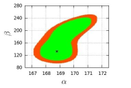
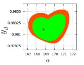
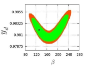
Figure 1: Allowed region for the three free parameters in the quark sector at $70\%$ (green) and $90\%$ (orange) confidence level.

4.2 PMNS mixing matrix

4.2.1 The masses of right-handed neutrinos with degeneration

As we observe from Eq. (41), the reactor and atmospheric angles turn out to be independent of the neutrino masses. These observables only depend explicitly on the $y_{\ell}$ free parameter, the charged lepton masses and the $\eta_{2e}$ Dirac phase; the latter may be ignored since we are only interested in the absolute values of the two mixing angles. On the other hand, the solar mixing angle depends on the $y_{\ell}$ free parameter, the $\bar{\eta}_{3e}$ phase, as well as the charged lepton and neutrino masses.

In order to show that in this model we can describe the lepton masses and mixing we will also make a $\chi^{2}$ fit using the theoretical expressions for the atmospheric and reactor angles given in Eq. (41) and compare them with the current experimental data for these mixing angles. Thus, for the atmospheric mixing angle we consider the following experimental value $\sin^{2}\theta^{\ell^{ex}}_{23}=0.52\pm 0.06$. Within this theoretical framework we will consider first the particular case when the first and second right-handed neutrinos are mass degenerate. In this case we can only determine a lower bound for the value of the reactor angle [50]. To perform the $\chi^{2}$ fit we considered the values for the reactor angle reported by the MINOS experiment; $\sin^{2}2\theta^{\ell^{ex}}_{13}=0.076\pm 0.068$. We considered also the following charged lepton masses values: $m_{e}=0.51099$ MeV, $m_{\mu}=105.6583$ MeV and $m_{\tau}=1776.82$ MeV [62]. As a result of this $\chi^{2}$ analysis, we obtained that for the best fit with $\chi^{2}=0.85$ as the minimum value, the free parameter $y_{\ell}$ at $1\sigma$ has the following range of values: $y_{\ell}=0.8478^{+0,0045}_{-0.0046}$. Moreover, the best theoretical values for the atmospheric and reactor angles that come from this analysis, at $1\sigma$, are:

$$\begin{array}[]{l}\vspace{2mm}\sin^{2}\theta^{\ell^{th}}_{23}=0.5206_{-0.0113}^{+0.0115}\rightarrow\theta^{\ell^{th}}_{23}=\left(46.18^{+0.66}_{-0.65}\right)^{\circ},\\ \sin^{2}2\theta^{\ell^{th}}_{13}=0.01386_{-0.00025}^{+0.00016}\rightarrow\theta^{\ell^{th}}_{13}=\left(3.38^{+0.03}_{-0.02}\right)^{\circ}.\end{array}$$ (56)

As can be observed, the atmospheric angle value is in good agreement with the experimental values, however, the obtained reactor mixing value is smaller than the central value obtained in the global fits. In fact, this theoretical value of the reactor angle is more than $3\sigma$ away from the values reported in ref. [68, 69]. But it is worth noting that our model predicts that the reactor angle must be different from zero and that is large in comparison to the one obtained from the tribimaximal mixing matrix. Moreover, as already stated above, it is a lower bound for the value obtained in a more general model where the right-handed neutrino masses are not degenerate. In figure 2, we show the dependence of the atmospheric and reactor angles on the parameter $y_{\ell}$.

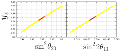
Figure 2: Atmospheric and reactor mixing angle values at $65\%$ (orange) and $95\%$ (yellow) of C.L.

Having determined the allowed values for the $y_{\ell}$ free parameter, then, the solar mixing angle just depends on the neutrino masses and one Dirac phase. We can reduce further the free parameters, noticing that the neutrino masses can be determined using the sum rule given in Eq. (36). This is written in terms of the observables $\Delta m^{2}_{\odot}$ and $\Delta m^{2}_{ATM}$ as

$$m_{\nu_{3}}\leq\left(\sqrt[4]{m^{2}_{\nu_{3}}+\Delta m^{2}_{\odot}+\Delta m^{2}_{\textrm{ATM}}}-\sqrt[4]{m^{2}_{\nu_{3}}+\Delta m^{2}_{\textrm{ATM}}}\right)^{2}.$$ (57)

From the above expression and using the experimental results of $\Delta m^{2}_{\odot}$ and $\Delta m^{2}_{ATM}$, we can get an upper bound for the $m_{\nu_{3}}$ lightest neutrino mass. Therefore, the allowed values for the lightest neutrino mass are: $0\leq m_{\nu_{3}}\leq 4\times 10^{-6}$ eV. As a result, the $m_{\nu_{2}}$ and $m_{\nu_{1}}$ neutrino masses are easily calculated in the following way

$$m_{\nu_{2}} = \sqrt{\Delta m^{2}_{\odot}+\Delta m^{2}_{\textrm{ATM}}}\sqrt{1+\dfrac{m^{2}_{\nu_{3}}}{\Delta m^{2}_{\odot}+\Delta m^{2}_{\textrm{ATM}}}}\approx 5.0\pm 0.087\times 10^{-2}~{}eV,$$

$$m_{\nu_{1}} = \sqrt{\Delta m^{2}_{\textrm{ATM}}}\sqrt{1+\dfrac{m^{2}_{\nu_{3}}}{\Delta m^{2}_{\textrm{ATM}}}}\approx 4.90\pm 0.089\times 10^{-2}~{}eV.$$ (58)

As we already commented, this version of our model where the first two RHN masses are degenerate, predicts an inverted ordering among the neutrino masses, the above values clarify explicitly our statement. Since we have calculated the neutrino masses, these cease to be considered as free parameters in the solar mixing angle expression given in Eq. (41). Furthermore, we obtain easily the solar mixing value that is allowed by the fixed free parameters, which are $y_{\ell}$ and the neutrino masses. Actually, with the particular value for the $\bar{\eta}_{3e}=\pi$ Dirac phase, and using the $y_{\ell}$ value at $90\%$ at C.L, we predict the following value for the solar mixing angle

$$\tan^{2}\theta^{\ell^{th}}_{12}=0.552\pm 0.078\rightarrow\theta^{\ell^{th}}_{12}=\left(36.62\pm 4.06\right)^{\circ}$$ (59)

where we have used $m_{\nu_{2}}=0.05080$ eV, $m_{\nu_{1}}=0.04987$ eV and $m_{\nu_{3}}=3.9\times 10^{-6}$ eV. As we observe the solar mixing angle value in Eq. (59) is in good agreement with the experimental data. In figure 3 we show explicitly the dependence of the solar angle on the $y_{\ell}$ parameter and the $m_{\nu_{3}}$ lightest neutrino mass, respectively.

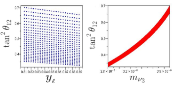
Figure 3: Solar mixing angle values as function of the $y_{\ell}$ parameter and the $m_{\nu_{3}}$ neutrino mass considering $m_{\nu_{2}}=0.05080$ eV, $m_{\nu_{1}}=0.04987$ eV and $\bar{\eta}_{3e}=\pi$.

It is clear from these results that the solar angle has a strong dependence on the $m_{\nu_{3}}$ mass, and that the sum rule for the neutrino masses does play an important role to determine the above mixing angle in good agreement with the experimental data.

4.2.2 The masses of right-handed neutrinos without degeneration

In the previous section we obtained that the reactor mixing angle, $\theta^{\ell}_{13}$, has a nonzero value, whereby the shape of lepton mixing matrix PMNS is not consistent with tribimaximal scenario. However, this value of the reactor mixing angle is small compared to the central value from the global fits [70], and would correspond to a lower bound.

Now, in order to reproduce the current numerical values of the reactor angle reported by global fits, we break the degeneration of the first two right-handed neutrinos, namely $M_{R_{1}}\neq M_{R_{2}}$. Also, we defined the $\chi^{2}$ function as:

$$\chi^{2}=\frac{\left(S_{12}^{2,ex}-S_{12}^{2,th}\right)^{2}}{\sigma_{S_{12}^{2,ex}}^{2}}+\frac{\left(S_{23}^{2,ex}-S_{23}^{2,th}\right)^{2}}{\sigma_{S_{23}^{2,ex}}^{2}}+\frac{\left(S_{13}^{2,ex}-S_{13}^{2,th}\right)^{2}}{\sigma_{S_{13}^{2,ex}}^{2}}$$ (60)

where $S_{ij}^{2,ex(th)}\equiv\sin^{2}\theta_{ij}^{\ell}$ with $i,j=1,2,3$. The terms with superindex $th$ are the theoretical expressions obtained from Eq. (49), while the terms with superindex $ex$ are the experimental data with uncertainty $\sigma_{S_{13}}$ given in Eq. (30). A consequence of considering the most general case with non-degenerate right- handed neutrino masses is an increasing of the number of free parameters in the PMNS matrix. In a first scan of the parameter space, we find that the $\eta_{1}$, $\alpha_{2}$, $\eta_{2e}$ and $\bar{\eta}_{3e}$ phases are not correlated among each other nor with the parameters $m_{\nu_{3[2]}}$, $\widetilde{\mu}_{0}$ and $\delta_{\nu}$. Thus we consider that the $\eta_{1}$, $\alpha_{2}$, $\eta_{2e}$ and $\bar{\eta}_{3e}$ phases vary in the range of 0 to $2\pi$. From the analysis done in the previous section we consider that $y_{\ell}\in\left[0.75,0.96\right]$. Then, to perform the $\chi^{2}$ fit the neutrino masses are written as:

$$\begin{array}[]{lll}\widetilde{m}_{\nu_{1}}=\dfrac{m_{\nu_{1}}}{m_{\nu_{3}}}=\sqrt{1-\frac{\Delta m^{2}_{\textrm{ATM}}}{m_{\nu_{3}}^{2}}},&\widetilde{m}_{\nu_{2}}=\dfrac{m_{\nu_{2}}}{m_{\nu_{3}}}=\sqrt{1-\frac{\Delta m^{2}_{32}}{m_{\nu_{3}}^{2}}}&\textrm{(NH),}\\ \widetilde{m}_{\nu_{3}}=\dfrac{m_{\nu_{3}}}{m_{\nu_{2}}}=\sqrt{1-\frac{\Delta m^{2}_{23}}{m_{\nu_{2}}}},&\widetilde{m}_{\nu_{1}}=\dfrac{m_{\nu_{1}}}{m_{\nu_{2}}}=\sqrt{1-\frac{\Delta m^{2}_{\odot}}{m_{\nu_{2}}^{2}}}&\textrm{(IH),}\end{array}$$ (61)

where $\Delta m^{2}_{32}=\Delta m^{2}_{\textrm{ATM}}-\Delta m^{2}_{\odot}$ and $\Delta m^{2}_{23}=\Delta m^{2}_{\textrm{ATM}}+\Delta m^{2}_{\odot}$. The upper [lower] row corresponds to a normal [inverted] hierarchy. The above expressions only have one free parameter which is $m_{\nu_{3[2]}}$. This parameter must satisfy the condition $m_{\nu_{3[2]}}<\Delta m^{2}_{32[\odot]}$ and $\sum_{i}m_{\nu_{i}}<0.23$ eV. The last one was reported by the Planck collaboration [71]. Thus in the $\chi^{2}$ fit we consider that $m_{\nu_{3[2]}}$ is not a free parameter, since it is constrained by experimental data. Thus, with $\theta=283^{\circ}[121^{\circ}]$ for a normal [inverted] hierarchy, we have that $\widetilde{\mu}_{0}$ and $\delta_{\nu}$ are the only free parameters in the fit.

Finally, as result of the $\chi^{2}$ analysis we obtained that for the best fit point $\chi^{2}=0.020[0.014]$ for a normal [inverted] hierarchy. Also, the neutrino masses at $1~{}\sigma$ are:

$$m_{\nu_{3}}=\left\{\begin{array}[]{l}\vspace{2mm}\left(5.35_{-1.73}^{+4.32}\right)\times 10^{-2}\textrm{eV}\\ \left(4.44_{-3.87}^{+4.21}\right)\times 10^{-2}\textrm{eV}\end{array}\right.,\,m_{\nu_{2}}=\left\{\begin{array}[]{l}\vspace{2mm}\left(2.01_{-0.98}^{+6.42}\right)\times 10^{-2}\textrm{eV}\\ \left(6.71_{-1.81}^{+3.25}\right)\times 10^{-2}\textrm{eV}\end{array}\right.,\,m_{\nu_{1}}=\left\{\begin{array}[]{l}\vspace{2mm}\left(1.08_{-1.30}^{+6.59}\right)\times 10^{-2}\textrm{eV}\\ \left(6.65_{-1.83}^{+3.27}\right)\times 10^{-2}\textrm{eV}\end{array}\right..$$ (68)

The free parameters $\widetilde{\mu}_{0}$ and $\delta_{\nu}$ at $1~{}\sigma$ are:

$$\begin{array}[]{l}\widetilde{\mu}_{0}=\left\{\begin{array}[]{l}\vspace{2mm}0.22_{-0.20}^{+0.63}\\ 0.56_{-0.56}^{+0.29}\end{array}\right.\quad\textrm{and}\quad\delta_{\nu}=\left\{\begin{array}[]{l}\vspace{2mm}0.75_{-0.15}^{+0.24}\\ 0.73_{-0.09}^{+0.25}\end{array}\right..\end{array}$$ (69)

We obtain the following numerical values for the leptonic mixing angles, at $1~{}\sigma$:

$$\begin{array}[]{l}\sin^{2}\theta_{12}^{\ell^{th}}=\left\{\begin{array}[]{l}\vspace{2mm}0.324_{-0.016}^{+0.015}\\ 0.325_{-0.018}^{+0.014}\end{array}\right.,\sin^{2}\theta_{23}^{\ell^{th}}=\left\{\begin{array}[]{l}\vspace{2mm}0.515_{-0.069}^{+0.078}\\ 0.562_{-0.048}^{+0.036}\end{array}\right.,\sin^{2}\theta_{13}^{\ell^{th}}=\left\{\begin{array}[]{l}\vspace{2mm}0.0232_{-0.0016}^{+0.0021}\\ 0.0241_{-0.0021}^{+0.0018}\end{array}\right.,\end{array}$$ (70)

$$\begin{array}[]{l}\theta_{12}^{\ell^{th}}=\left\{\begin{array}[]{l}\vspace{2mm}\left(34.71_{-0.98}^{+0.91}\right)^{\circ}\\ \left(34.73_{-1.11}^{+0.89}\right)^{\circ}\end{array}\right.,\theta_{23}^{\ell^{th}}=\left\{\begin{array}[]{l}\vspace{2mm}\left(45.83_{-3.98}^{+4.49}\right)^{\circ}\\ \left(48.57_{-2.76}^{+2.07}\right)^{\circ}\end{array}\right.,\theta_{13}^{\ell^{th}}=\left\{\begin{array}[]{l}\vspace{2mm}\left(8.77_{-0.32}^{+0.40}\right)^{\circ}\\ \left(8.93_{-0.39}^{+0.33}\right)^{\circ}\end{array}\right.,\end{array}$$ (71)

which are in very good agreement with the last global fit reported in Ref [70]. The upper (lower) row corresponds to a normal (inverted) hierarchy. In the figure 4 we show the allowed regions, at $69\%$ and $95\%$ C.L., for the sine-squared of the lepton mixing angles considering a normal and inverted hierarchy.

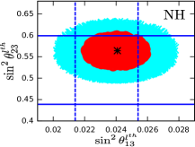
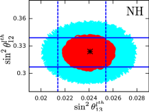
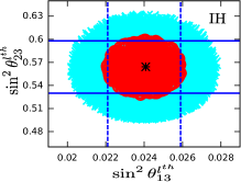
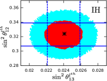
Figure 4: Allowed regions for the lepton mixing angles considering a normal and inverted hierarchy (NH and IH) in the mass spectrum of neutrinos. The turquoise region is at $90\%$, the red region is at $69\%$. The blue solid lines delimit the experimental data of $\sin^{2}\theta_{12(23)}^{\ell}$ at $1\sigma$. The blue dashed lines delimit the experimental data of $\sin^{2}\theta_{13}^{\ell}$ at $1\sigma$ [70].

Before closing this section, a relevant comment is in order. As it is well known, the effective neutrino mass matrix, $\bf{M}_{\nu}$, is sensitive to the effect of the running of the mass matrix parameters from high to low energy [72, 73]. Actually, small mixing angles could get a notable enhancement as was remarked in [72]. Thus, in the scenario where the $\theta_{13}$ is tiny, it would be interesting to make a running of the mixing parameters to know how much the reactor angle changes, but we will leave this for a future work.

5 Outlook and Remarks

We have studied a non-minimal supersymmetric $SU(5)$ model where the $Q_{6}$ flavour symmetry plays an important role in accommodating the masses and mixings for quarks an leptons. For the former sector, the CKM mixing matrix has been obtained with great accuracy and it is consistent with the experimental results. For leptons we considered two cases: $a)$ the first two masses of RHN’s are degenerate. $b)$ the RHN’s masses are not degenerate.

On the one hand, for the case $a)$ the flavour symmetry implies an appealing sum rule for the neutrino masses, which leads to an inverted hierarchy and is crucial to determine the solar mixing angle. As a main result in this case, we have that the atmospheric $\theta^{\ell^{th}}_{23}=\left(46.18^{+0.66}_{-0.65}\right)^{\circ}$ and solar angle $\theta^{\ell^{th}}_{12}=\left(36.62\pm 4.06\right)^{\circ}$ are in good agreement with the experimental data, however, the reactor angle value, $\theta^{\ell^{th}}_{13}=\left(3.38^{+0.03}_{-0.02}\right)^{\circ}$, is more than $3\sigma$ away from the central value from the global fits. It is worth pointing out that the model predicts a non-zero value for this angle, unlike the tri-bimaximal case, and that this value constitutes the lower bound for $\theta_{13}$ in the more general model, where the right-handed neutrinos in the $Q_{6}$ doublet are not mass degenerate.

On the other hand, for the more general case $b)$, where the RHN’s masses are not degenerate, we obtained a value for the reactor mixing angle in very good agreement with the last experimental data or global fits, as is the case in the non-supersymmetric $S_{3}$ models [50]. Namely, in this case it is possible that the neutrino mass spectrum obeys a normal or an inverted hierarchy. Thus, we obtain that the leptonic mixing angles have the following theoretical values for a normal [inverted] hierarchy: $\theta_{12}^{\ell^{th}}=\left(34.71_{-0.98}^{+0.91}\right)^{\circ}$ $\left[\left(34.73_{-1.11}^{+0.89}\right)^{\circ}\right]$, $\theta_{23}^{\ell^{th}}=\left(45.83_{-3.98}^{+4.49}\right)^{\circ}$ $\left[\left(48.57_{-2.76}^{+2.07}\right)^{\circ}\right]$, and $\theta_{13}^{\ell^{th}}=\left(8.77_{-0.32}^{+0.40}\right)^{\circ}$ $\left[\left(8.93_{-0.39}^{+0.33}\right)^{\circ}\right]$.

Although in this preliminary analysis we have found the form of the mass and mixing matrices for quarks and leptons and we have shown that they lead to realistic values, we have left aside subtle issues as the full analysis of the scalar superpotential, the details of the proton decay, the running of the mass parameters from high to low scale energy, and all the phenomenology that the model provides by itself. These topics will be taken into account in a complete study of the model, as we already commented. In general, the model seems to work out very well and it may be considered as a realistic one.

Appendix A $Q_{6}$ Flavour symmetry

The $Q_{6}$ group has twelve elements which are contained in six conjugacy classes, therefore, it contains six irreducible representations. We will use the notation given in [15], there are various notations and extensive studies for this group, see for example [74, 12]. The $Q_{6}$ family symmetry has ${\bf 2}$ two-dimensional irreducible representations denoted by ${\bf 2}_{1}$ and ${\bf 2}_{2}$, $4$ one-dimensional ones which are denoted by ${\bf 1}_{+,0}$, ${\bf 1}_{+,2}$, ${\bf 1}_{-,1}$ and ${\bf 1}_{-,3}$. As it is well known, ${\bf 2}_{1}$ is a pseudo real and ${\bf 2}_{2}$ is a real representation. In addition, for ${\bf 1}_{\pm,n}$ we have that $n=0,1,2,3$ is the factor $\exp\left(in\pi/2\right)$ that appears in the matrix given by ${\bf B}$. The $\pm$ stands for the change of sign under the transformation given by the ${\bf A}$ matrix. So that the first two one-dimensional representations are real and the two latter ones are complex conjugate to each other.

$$Q_{6}=\{1,{\bf A},{\bf A}^{2},{\bf A}^{3},{\bf A}^{4},{\bf A}^{5},{\bf B},{\bf A}{\bf B},{\bf A}^{2}{\bf B},{\bf A}^{3}{\bf B},{\bf A}^{4}{\bf B},{\bf A}^{5}{\bf B}\},$$ (72)

where the ${\bf A}$ and ${\bf B}$ are two-dimensional matrices whose explicit forms are given by

$${\bf A}=\begin{pmatrix}\cos\left(\pi/3\right)&\sin\left(\pi/3\right)\\ -\sin\left(\pi/3\right)&\cos\left(\pi/3\right)\end{pmatrix}\quad\textrm{and}\quad{\bf B}=\begin{pmatrix}i&0\\ 0&-i\end{pmatrix}.$$ (73)

Let us write the multiplication rules among the six irreducible representations which will be useful to build a phenomenological model:

$${\bf 1}_{+,2}\otimes{\bf 1}_{+,2} ={\bf 1}_{+,0},\quad{\bf 1}_{-,3}\otimes{\bf 1}_{-,3}={\bf 1}_{+,2},\quad{\bf 1}_{-,1}\otimes{\bf 1}_{-,1}={\bf 1}_{+,2},\quad{\bf 1}_{-,1}\otimes{\bf 1}_{-,3}={\bf 1}_{+,0},$$

$${\bf 1}_{+,2}\otimes{\bf 1}_{-,1} ={\bf 1}_{-,3},\quad{\bf 1}_{+,2}\otimes{\bf 1}_{-,3}={\bf 1}_{-,1},\quad{\bf 2}_{1}\otimes{\bf 1}_{+,2}={\bf 2}_{1},\quad{\bf 2}_{1}\otimes{\bf 1}_{-,3}={\bf 2}_{2},$$

$${\bf 2}_{1}\otimes{\bf 1}_{-,1} ={\bf 2}_{2},\quad{\bf 2}_{2}\otimes{\bf 1}_{+,2}={\bf 2}_{2},\quad{\bf 2}_{2}\otimes{\bf 1}_{-,3}={\bf 2}_{1},\quad{\bf 2}_{2}\otimes{\bf 1}_{-,1}={\bf 2}_{1};$$

$$\overbrace{\begin{pmatrix}x_{1}\\ x_{2}\end{pmatrix}}^{{\bf 2}_{1}}\,\otimes\,\overbrace{\begin{pmatrix}y_{1}\\ y_{2}\end{pmatrix}}^{{\bf 2}_{1}} =\overbrace{\left(x_{1}y_{2}-x_{2}y_{1}\right)}^{{\bf 1}_{+,0}}\quad+\quad\overbrace{\left(x_{1}y_{1}+x_{2}y_{2}\right)}^{{\bf 1}_{+,2}}\quad+\quad\overbrace{\begin{pmatrix}-x_{1}y_{2}-x_{2}y_{1}\\ x_{1}y_{1}-x_{2}y_{2}\end{pmatrix}}^{{\bf 2}_{2}}$$

$$\overbrace{\begin{pmatrix}a_{1}\\ a_{2}\end{pmatrix}}^{{\bf 2}_{2}}\otimes\overbrace{\begin{pmatrix}b_{1}\\ b_{2}\end{pmatrix}}^{{\bf 2}_{2}} =\overbrace{\left(a_{1}b_{1}+a_{2}b_{2}\right)}^{{\bf 1}_{+,0}}\quad+\quad\overbrace{\left(a_{1}b_{2}-a_{2}b_{1}\right)}^{{\bf 1}_{+,2}}\quad+\quad\overbrace{\begin{pmatrix}-a_{1}b_{1}+a_{2}b_{2}\\ a_{1}b_{2}+a_{2}b_{1}\end{pmatrix}}^{{\bf 2}_{2}}$$

$$\overbrace{\begin{pmatrix}x_{1}\\ x_{2}\end{pmatrix}}^{{\bf 2}_{1}}\otimes\overbrace{\begin{pmatrix}a_{1}\\ a_{2}\end{pmatrix}}^{{\bf 2}_{2}} =\overbrace{\left(x_{1}a_{2}+x_{2}a_{1}\right)}^{{\bf 1}_{-,3}}\quad+\quad\overbrace{\left(x_{1}a_{1}-x_{2}a_{2}\right)}^{{\bf 1}_{-,1}}\quad+\quad\overbrace{\begin{pmatrix}x_{1}a_{1}+x_{2}a_{2}\\ x_{1}a_{2}-x_{2}a_{1}\end{pmatrix}}^{{\bf 2}_{1}},$$ (74)

Appendix B Neutrino Mass Matrix

The degeneracy in the vacuum expectation values for two scalar fields, does not modify the functional structure of the effective neutrino mass matrix ${\bf m}_{\nu}$, eq. (16), because it still is a matrix with one texture zero. But the parameters $a_{\nu}$, $b_{\nu}$, $c_{\nu}$, $d_{\nu}$ and $\mu_{0}$ given in eq. (17) are simplified a little. Therefore, the expressions in eqs (16) and (17) take the following form

$${\bf m}_{\nu}={\bf\textit{u}}_{\theta}^{T}{\bf M}_{\nu}{\bf\textit{u}}_{\theta}=\left(\begin{array}[]{ccc}b_{\nu}&a_{\nu}&c_{\nu}\\ a_{\nu}&\mu_{0}&0\\ c_{\nu}&0&d_{\nu}\end{array}\right)\quad\textrm{and}\quad{\bf\textit{u}}_{\theta}=\left(\begin{array}[]{ccc}\cos\theta&0&-\sin\theta\\ \sin\theta&0&\cos\theta\\ 0&1&0\end{array}\right),$$ (75)

with

$$\begin{array}[]{l}\vspace{2mm}\tan\theta=\frac{M_{R_{2}}}{M_{R_{1}}},\quad\mu_{0}=\frac{\left(y_{2}^{n}h^{0u}\right)^{2}}{M_{R_{1}}M_{R_{2}}}\left[M_{R_{2}}+M_{R_{1}}\right],\quad a_{\nu}=\frac{\cos\theta y_{1}^{n}h^{0u}_{3}y_{2}^{n}h^{0u}}{M_{R_{2}}M_{R_{1}}^{2}}\left(M_{R_{1}}^{2}+M_{R_{2}}^{2}\right),\\ \vspace{2mm}b_{\nu}=\frac{\cos^{2}\theta}{M_{R_{1}}^{2}}\left[\frac{\left(y_{1}^{n}h^{0u}_{3}\right)^{2}}{M_{R_{1}}M_{R_{2}}}\left(M_{R_{1}}^{3}+M_{R_{2}}^{3}\right)+\frac{\left(y_{3}^{n}h^{0u}\right)^{2}}{M_{R_{3}}}\left(M_{R_{1}}+M_{R_{2}}\right)^{2}\right],\\ \vspace{2mm}c_{\nu}=\frac{\cos^{2}\theta}{M_{R_{1}}^{2}}\left[\left(y_{1}^{n}h^{0u}_{3}\right)^{2}\left(M_{R_{2}}-M_{R_{1}}\right)+\frac{\left(y_{3}^{n}h^{0u}\right)^{2}}{M_{R_{3}}}\left(M_{R_{1}}^{2}-M_{R_{2}}^{2}\right)\right],\;\textrm{and}\\ \vspace{2mm}d_{\nu}=\frac{\cos^{2}\theta}{\left(M_{R_{1}}\right)^{2}}\left[\left(y_{1}^{n}h^{0u}_{3}\right)^{2}\left(M_{R_{2}}+M_{R_{1}}\right)+\frac{\left(y_{3}^{n}h^{0u}\right)^{2}}{M_{R_{3}}}\left(M_{R_{1}}-M_{R_{2}}\right)^{2}\right].\end{array}$$ (76)

From the previous expressions is easy to notice that when the masses of the first two right-handed neutrinos are degenerate, $M_{R_{1}}=M_{R_{2}}$, the parameter $c_{\nu}$ becomes zero and the rotation angle takes the value $\theta=\pi/4$. Hence, the effective neutrino mass matrix ${\bf m}_{\nu}$ is reduced to a block matrix.

References

- [1] A. Masiero, S. K. Vempati, and O. Vives. Flavour physics and grand unification. 0711.2903, 2005.
- [2] H. Fritzsch. Calculating the Cabibbo Angle. Phys.Lett., B70:436, 1977.
- [3] H. Fritzsch. Weak Interaction Mixing in the Six - Quark Theory. Phys.Lett., B73:317–322, 1978.
- [4] Makoto Kobayashi and Toshihide Maskawa. CP Violation in the Renormalizable Theory of Weak Interaction. Prog. Theor. Phys., 49:652–657, 1973.
- [5] Nicola Cabibbo. Unitary Symmetry and Leptonic Decays. Phys.Rev.Lett., 10:531–533, 1963.
- [6] G. C. Branco, D. Emmanuel-Costa, and C. Simoes. Nearest-Neighbour Interaction from an Abelian Symmetry and Deviations from Hermiticity. Phys. Lett., B690:62–67, 2010.
- [7] Harald Fritzsch, Zhi-zhong Xing, and Ye-Ling Zhou. Non-Hermitian Perturbations to the Fritzsch Textures of Lepton and Quark Mass Matrices. Phys. Lett., B697:357–363, 2011.
- [8] Ziro Maki, Masami Nakagawa, and Shoichi Sakata. Remarks on the unified model of elementary particles. Prog.Theor.Phys., 28:870–880, 1962.
- [9] B. Pontecorvo. Neutrino experiments and the question of leptonic-charge conservation. Sov. Phys. JETP, 26:984–988, 1968.
- [10] K. Harayama and N. Okamura. Exact parametrization of the mass matrices and the KM matrix. Phys.Lett., B387:614–622, 1996.
- [11] K. Harayama, N. Okamura, A.I. Sanda, and Zhi-Zhong Xing. Getting at the quark mass matrices. Prog.Theor.Phys., 97:781–790, 1997.
- [12] Hajime Ishimori, Tatsuo Kobayashi, Hiroshi Ohki, Yusuke Shimizu, Hiroshi Okada, and Morimitsu Tanimoto. Non-abelian discrete symmetries in particle physics. Progress of Theoretical Physics Supplement, 183:1–163, 2010.
- [13] Kaladi S. Babu and Jisuke Kubo. Dihedral families of quarks, leptons and Higgses. Phys.Rev., D71:056006, 2005.
- [14] Yuji Kajiyama, Etsuko Itou, and Jisuke Kubo. Nonabelian discrete family symmetry to soften the SUSY flavor problem and to suppress proton decay. Nucl. Phys., B743:74–103, 2006.
- [15] Yuji Kajiyama. R-parity violation and non-Abelian discrete family symmetry. JHEP, 04:007, 2007.
- [16] K.S. Babu and Yanzhi Meng. Flavor Violation in Supersymmetric Q(6) Model. Phys.Rev., D80:075003, 2009.
- [17] K.S. Babu, Kenji Kawashima, and Jisuke Kubo. Variations on the Supersymmetric Model of Flavor. Phys.Rev., D83:095008, 2011.
- [18] H. Georgi, Helen R. Quinn, and Steven Weinberg. Hierarchy of Interactions in Unified Gauge Theories. Phys.Rev.Lett., 33:451–454, 1974.
- [19] Jogesh C. Pati and Abdus Salam. Lepton Number as the Fourth Color. Phys.Rev., D10:275–289, 1974.
- [20] R.N. Mohapatra and Jogesh C. Pati. A Natural Left-Right Symmetry. Phys.Rev., D11:2558, 1975.
- [21] H. Georgi and S.L. Glashow. Unity of All Elementary Particle Forces. Phys.Rev.Lett., 32:438–441, 1974.
- [22] Paul Langacker. Grand Unified Theories and Proton Decay. Phys. Rept., 72:185, 1981.
- [23] A. J. Buras, John R. Ellis, M. K. Gaillard, and Dimitri V. Nanopoulos. Aspects of the Grand Unification of Strong, Weak and Electromagnetic Interactions. Nucl. Phys., B135:66–92, 1978.
- [24] Savas Dimopoulos and Howard Georgi. Softly Broken Supersymmetry and SU(5). Nucl.Phys., B193:150, 1981.
- [25] S. Dimopoulos, S. Raby, and Frank Wilczek. Supersymmetry and the Scale of Unification. Phys.Rev., D24:1681–1683, 1981.
- [26] N. Sakai. Naturalness in Supersymmetric Guts. Z.Phys., C11:153, 1981.
- [27] N. Sakai and Tsutomu Yanagida. Proton Decay in a Class of Supersymmetric Grand Unified Models. Nucl.Phys., B197:533, 1982.
- [28] Steven Weinberg. Supersymmetry at Ordinary Energies. 1. Masses and Conservation Laws. Phys.Rev., D26:287, 1982.
- [29] John R. Ellis, Dimitri V. Nanopoulos, and Serge Rudaz. GUTs 3: SUSY GUTs 2. Nucl. Phys., B202:43, 1982.
- [30] Savas Dimopoulos, Stuart Raby, and Frank Wilczek. Proton Decay in Supersymmetric Models. Phys.Lett., B112:133, 1982.
- [31] Pran Nath, Ali H. Chamseddine, and Richard L. Arnowitt. Nucleon Decay in Supergravity Unified Theories. Phys.Rev., D32:2348–2358, 1985.
- [32] J. Hisano, H. Murayama, and T. Yanagida. Nucleon decay in the minimal supersymmetric SU(5) grand unification. Nucl.Phys., B402:46–84, 1993.
- [33] Toru Goto and Takeshi Nihei. Effect of RRRR dimension five operator on the proton decay in the minimal SU(5) SUGRA GUT model. Phys.Rev., D59:115009, 1999.
- [34] Hitoshi Murayama and Aaron Pierce. Not even decoupling can save minimal supersymmetric SU(5). Phys.Rev., D65:055009, 2002.
- [35] Borut Bajc, Pavel Fileviez Perez, and Goran Senjanovic. Proton decay in minimal supersymmetric SU(5). Phys.Rev., D66:075005, 2002.
- [36] W. Martens, L. Mihaila, J. Salomon, and M. Steinhauser. Minimal Supersymmetric SU(5) and Gauge Coupling Unification at Three Loops. Phys.Rev., D82:095013, 2010.
- [37] Junji Hisano, Daiki Kobayashi, Takumi Kuwahara, and Natsumi Nagata. Decoupling Can Revive Minimal Supersymmetric SU(5). JHEP, 1307:038, 2013.
- [38] J. C. Romao and J. W. F. Valle. Neutrino masses in supersymmetry with spontaneously broken R parity. Nucl. Phys., B381:87–108, 1992.
- [39] M. Hirsch, M.A. Diaz, W. Porod, J.C. Romao, and J.W.F. Valle. Neutrino masses and mixings from supersymmetry with bilinear R parity violation: A Theory for solar and atmospheric neutrino oscillations. Phys.Rev., D62:113008, 2000.
- [40] Murray Gell-Mann, Pierre Ramond, and Richard Slansky. Complex Spinors and Unified Theories. Conf.Proc., C790927:315–321, 1979.
- [41] M. Fukugita and T. Yanagida. Physics of Neutrinos: And Applications to Astrophysics. Physics and astronomy online library. Springer, 2003.
- [42] Rabindra N. Mohapatra and Goran Senjanovic. Neutrino Masses and Mixings in Gauge Models with Spontaneous Parity Violation. Phys. Rev., D23:165, 1981.
- [43] Rabindra N. Mohapatra and Goran Senjanovic. Neutrino Mass and Spontaneous Parity Violation. Phys.Rev.Lett., 44:912, 1980.
- [44] Peter Minkowski. mu e gamma at a Rate of One Out of 1-Billion Muon Decays? Phys. Lett., B67:421, 1977.
- [45] Hajime Ishimori, Yusuke Shimizu, and Morimitsu Tanimoto. S4 Flavor Symmetry of Quarks and Leptons in SU(5) GUT. Prog. Theor. Phys., 121:769–787, 2009.
- [46] Claudia Hagedorn, Stephen F. King, and Christoph Luhn. A SUSY GUT of Flavour with S4 x SU(5) to NLO. JHEP, 06:048, 2010.
- [47] Mu-Chun Chen, Jinrui Huang, K.T. Mahanthappa, and Alexander M. Wijangco. Large in a SUSY SU(5) x T’ Model. JHEP, 1310:112, 2013.
- [48] O. Felix, A. Mondragon, M. Mondragon, and E. Peinado. Neutrino masses and mixings in a minimal S(3)-invariant extension of the standard model. AIP Conf. Proc., 917:383–389, 2007.
- [49] A. Mondragon, M. Mondragon, and E. Peinado. Lepton masses, mixings and FCNC in a minimal -invariant extension of the Standard Model. Phys. Rev., D76:076003, 2007.
- [50] F. Gonzalez Canales, A. Mondragon, and M. Mondragon. The Flavour Symmetry: Neutrino Masses and Mixings. Fortsch.Phys., 61:546–570, 2013.
- [51] M.B. Einhorn and D.R.T. Jones. The Weak Mixing Angle and Unification Mass in Supersymmetric SU(5). Nucl.Phys., B196:475, 1982.
- [52] F. Astorga. Constraints from unification in SU(5) and SUSY SU(5). J.Phys., G20:241–260, 1994.
- [53] Z. Berezhiani, Z. Tavartkiladze, and M. Vysotsky. d = 5 operators in SUSY GUT: Fermion masses versus proton decay. arXiv:hep-ph/9809301, 1998.
- [54] Borut Bajc, Pavel Fileviez Perez, and Goran Senjanovic. Minimal supersymmetric su(5) theory and proton decay: Where do we stand? pages 131–139, 2002.
- [55] Ilja Dorsner and Irina Mocioiu. Predictions from type II see-saw mechanism in SU(5). Nucl.Phys., B796:123–136, 2008.
- [56] Harald Fritzsch and Zhi-zhong Xing. Mass and flavor mixing schemes of quarks and leptons. Prog. Part. Nucl. Phys., 45:1–81, 2000.
- [57] F. Gonz lez Canales, A. Mondrag n, M. Mondrag n, U.J. Salda a Salazar, and L. Velasco-Sevilla. Fermion mixing in an model with three Higgs doublets. J.Phys.Conf.Ser., 447:012053, 2013.
- [58] F. Gonzalez Canales and A. Mondragon. The neutrino mixing angle theta(13) in an S(3) flavour symmetric model. J.Phys.Conf.Ser., 387:012008, 2012.
- [59] F. Gonzalez Canales and A. Mondragon. The flavour symmetry S(3) and the neutrino mass matrix with two texture zeroes. J.Phys.Conf.Ser., 378:012014, 2012.
- [60] F. Gonz lez Canales, A. Mondrag n, M. Mondrag n, U. J. Salda a Salazar, and L. Velasco-Sevilla. Quark sector of S3 models: classification and comparison with experimental data. Phys.Rev., D88:096004, 2013.
- [61] F. Gonzalez Canales and A. Mondragon. The symmetry: Flavour and texture zeroes. J. Phys. Conf. Ser., 287:012015, 2011.
- [62] K. Nakamura et al. Review of particle physics. J. Phys., G37:075021, 2010.
- [63] Thomas Schwetz, Mariam Tortola, and J.W.F. Valle. Global neutrino data and recent reactor fluxes: status of three-flavour oscillation parameters. New J.Phys., 13:063004, 2011. * Temporary entry *.
- [64] P. Adamson et al. Improved search for muon-neutrino to electron-neutrino oscillations in MINOS. Phys.Rev.Lett., 107:181802, 2011.
- [65] J. Beringer et al. Review of Particle Physics (RPP). Phys.Rev., D86:010001, 2012.
- [66] Zhi-zhong Xing, He Zhang, and Shun Zhou. Updated Values of Running Quark and Lepton Masses. Phys.Rev., D77:113016, 2008.
- [67] F. Gonzalez Canales, A. Mondragon, U.J. Saldana Salazar, and L. Velasco-Sevilla. as a unified family theory for quarks and leptons. arXiv:1210.0288, 2012.
- [68] D.V. Forero, M. Tortola, and J.W.F. Valle. Global status of neutrino oscillation parameters after Neutrino-2012. Phys.Rev., D86:073012, 2012.
- [69] M.C. Gonzalez-Garcia, Michele Maltoni, Jordi Salvado, and Thomas Schwetz. Global fit to three neutrino mixing: critical look at present precision. JHEP, 1212:123, 2012.
- [70] D.V. Forero, M. Tortola, and J.W.F. Valle. Neutrino oscillations refitted. arXiv:1405.7540, 2014.
- [71] P.A.R. Ade et al. Planck 2013 results. XVI. Cosmological parameters. Astron.Astrophys., 2014.
- [72] K.S. Babu, Chung Ngoc Leung, and James T. Pantaleone. Renormalization of the neutrino mass operator. Phys.Lett., B319:191–198, 1993.
- [73] Shamayita Ray. Renormalization group evolution of neutrino masses and mixing in seesaw models: A Review. Int.J.Mod.Phys., A25:4339–4384, 2010.
- [74] Jisuke Kubo. Super Flavorsymmetry with Multiple Higgs Doublets. Fortsch.Phys., 61:597–621, 2013.