Distributed Robust Consensus Control of Multi-agent Systems with Heterogeneous Matching Uncertainties

Abstract

This paper considers the distributed consensus problem of linear multi-agent systems subject to different matching uncertainties for both the cases without and with a leader of bounded unknown control input. Due to the existence of nonidentical uncertainties, the multi-agent systems discussed in this paper are essentially heterogeneous. For the case where the communication graph is undirected and connected, a distributed continuous static consensus protocol based on the relative state information is first designed, under which the consensus error is uniformly ultimately bounded and exponentially converges to a small adjustable residual set. A fully distributed adaptive consensus protocol is then designed, which, contrary to the static protocol, relies on neither the eigenvalues of the Laplacian matrix nor the upper bounds of the uncertainties. For the case where there exists a leader whose control input is unknown and bounded, distributed static and adaptive consensus protocols are proposed to ensure the boundedness of the consensus error. It is also shown that the proposed protocols can be redesigned so as to ensure the boundedness of the consensus error in the presence of bounded external disturbances which do not satisfy the matching condition. A sufficient condition for the existence of the proposed protocols is that each agent is stabilizable.

, , [cor]Corresponding author.

1 Introduction

Cooperative control of a network of autonomous agents has been an emerging research direction and attracted a lot of attention from many scientific communities, especially the systems and control community. A group of autonomous agents, by coordinating with each other via communication or sensing networks, can perform certain challenging tasks which cannot be well accomplished by a single agent. Cooperative control of multi-agent systems has potential applications in broad areas including spacecraft formation flying, sensor networks, and cooperative surveillance [1, 2]. In the area of cooperative control, consensus is an important and fundamental problem, which means to develop distributed control policies using only local information to ensure that the agents reach an agreement on certain quantities of interest.

Two pioneering works on consensus are [3] and [4]. A theoretical explanation is provided in [3] for the alignment behavior observed in the Vicsek model [5] and a general framework of the consensus problem for networks of integrators is proposed in [4]. Since then, the consensus problem has been extensively studied by various scholars from different perspectives; see [1, 2, 6, 7, 8, 9, 10, 11, 12] and references therein. Existing consensus algorithms can be roughly categorized into two classes, namely, consensus without a leader (i.e., leaderless consensus) and consensus with a leader. The latter is also called leader-follower consensus or distributed tracking. In [6], a sufficient condition is derived to achieve consensus for multi-agent systems with jointly connected communication graphs. The authors in [7] design a distributed neighbor-based estimator to track an active leader. Distributed tracking algorithms are proposed in [13] and [14] for a network of agents with first-order dynamics. Consensus of networks of double- and high-order integrators is studied in [15, 16]. Consensus algorithms are designed in [8, 17] for multi-agent systems with quantized communication links. The authors in [18] address a distributed tracking problem for multiple Euler-Lagrange systems with a dynamic leader. The consensus problem of multi-agent systems with general discrete- and continuous-time linear dynamics is studied in [9, 10, 11, 12, 19, 20, 21]. It is worth noting that the design of the consensus protocols in [9, 10, 11, 20, 21] requires the knowledge of the eigenvalues of the Laplacian matrix of the communication graph, which is actually global information. To overcome this limitation, distributed adaptive consensus protocols are proposed in [22, 23]. For the case where there exists a leader with possibly nonzero control input, distributed controllers are proposed in [24, 23] to solve the leader-follower consensus problem. A common assumption in [9, 10, 11, 12, 19, 20, 21, 24, 23] is that the dynamics of the agents are identical and precisely known, which might be restrictive and not practical in many circumstances. In practical applications, the agents may be subject to certain parameter uncertainties or unknown external disturbances.

This paper considers the distributed consensus problem of multi-agent systems with identical nominal linear dynamics but subject to different matching uncertainties. A typical example belonging to this scenario is a network of mass-spring systems with different masses or unknown spring constants. Due to the existence of the nonidentical uncertainties which may be time-varying, nonlinear and unknown, the multi-agent systems discussed in this paper are essentially heterogeneous. The heterogeneous multi-agent systems in this paper contain the homogeneous linear multi-agent systems studied in [9, 10, 11, 12, 19, 20, 21] as a special case where the uncertainties do not exist. Note that because of the existence of the uncertainties, the consensus problem in this case becomes quite challenging to solve and the consensus algorithms given in [9, 10, 11, 12, 19, 20, 21] are not applicable any more.

In this paper, we present a systematic procedure to address the distributed robust consensus problem of multi-agent systems with matching uncertainties for both the cases without and with a leader of possibly nonzero control input. First, we consider the case where the communication graph is undirected and connected. A distributed continuous static consensus protocol based on the relative states of neighboring agents is designed, under which the consensus error is uniformly ultimately bounded and exponentially converges to a small residual set. Note that the design of this protocol relies on the eigenvalues of the Laplacian matrix and the upper bounds of the matching uncertainties. In order to remove these requirements, a fully distributed adaptive protocol is further designed, under which the residual set of the consensus error is also given. One desirable feature is that for both the static and adaptive protocols, the residual sets of the consensus error can be made to be reasonably small by properly selecting the design parameters of the protocols and the convergence rates of the consensus error are explicitly given. Next, we extend to consider the case where there exists a leader with nonzero control input. Here we study the general case where the leader’s control input is not available to any follower, which imposes additional difficulty. Distributed static and adaptive consensus protocols based on the relative state information are proposed and designed to ensure that the consensus error can converge to residual sets which are explicitly given and adjustable. The case where the external disturbances associated with the agent dynamics are bounded and do not satisfy the matching condition is also examined. The proposed consensus protocols are redesigned to guarantee the boundedness of the consensus error. The existence conditions of the consensus protocols proposed in this paper are discussed. It is pointed out that a sufficient condition of the existence of the protocols is that each agent is stabilizable.

It is worth mentioning that in related works [25, 26], the distributed tracking problem of multi-agent systems with unknown nonlinear dynamics are discussed. Compared to [25, 26], the contribution of this paper is at least three-fold. First, the agents in [25, 26] are restricted to be first-order and special high-order systems. It is far from trivial to extend [25, 26] to solve the consensus problem of the general high-order multi-agent systems with matching uncertainties as in this paper. Second, contrary to [25, 26] which consider only the case with a leader, consensus for both the cases with and without a leader is addressed in this paper. Third, the design of the protocols in [25, 26] depends on global information of the communication graph. In contrast, the adaptive consensus protocols proposed in this paper are fully distributed, which do not require any global information.

The rest of this paper is organized as follows. Some useful results of graph theory are reviewed in Section 2. The distributed robust leaderless consensus problem is discussed in Section 3 for the case with an undirected graph. The robust leader-follower consensus problem is addressed in Section 4 for the case where there exists a leader with unknown control input. The robustness of the proposed consensus protocols with respect to external disturbances which do not satisfy the matching condition is discussed in Section 5. Simulation examples are presented for illustration in Section 6. Conclusions are drawn in Section 7.

2 Notation and Graph Theory

$I_{N}$ represents the identity matrix of dimension $N$. Denote by $\mathbf{1}$ a column vector with all entries equal to one. ${\rm{diag}}(A_{1},\cdots,A_{n})$ represents a block-diagonal matrix with matrices $A_{i},i=1,\cdots,n,$ on its diagonal. $A\otimes B$ denotes the Kronecker product of matrices $A$ and $B$. For a vector $x\in\mathbf{R}^{n}$, let $\|x\|$ denote its 2-norm. For a symmetric matrix $A$, $\lambda_{\min}(A)$ and $\lambda_{\max}(A)$ denote, respectively, the minimum and maximum eigenvalues of $A$.

A directed graph $\mathcal{G}$ is a pair $(\mathcal{V},\mathcal{E})$, where $\mathcal{V}=\{v_{1},\cdots,v_{N}\}$ is a nonempty finite set of nodes and $\mathcal{E}\subseteq\mathcal{V}\times\mathcal{V}$ is a set of edges, in which an edge is represented by an ordered pair of distinct nodes. For an edge $(v_{i},v_{j})$, node $v_{i}$ is called the parent node, node $v_{j}$ the child node, and $v_{i}$ is a neighbor of $v_{j}$. A graph with the property that $(v_{i},v_{j})\in\mathcal{E}$ implies $(v_{j},v_{i})\in\mathcal{E}$ for any $v_{i},v_{j}\in\mathcal{V}$ is said to be undirected. A path from node $v_{i_{1}}$ to node $v_{i_{l}}$ is a sequence of ordered edges of the form $(v_{i_{k}},v_{i_{k+1}})$, $k=1,\cdots,l-1$. A subgraph $\mathcal{G}_{s}=(\mathcal{V}_{s},\mathcal{E}_{s})$ of $\mathcal{G}$ is a graph such that $\mathcal{V}_{s}\subseteq\mathcal{V}$ and $\mathcal{E}_{s}\subseteq\mathcal{E}$. A directed graph contains a directed spanning tree if there exists a node called the root, which has no parent node, such that the node has directed paths to all other nodes in the graph.

The adjacency matrix $\mathcal{A}=[a_{ij}]\in\mathbf{R}^{N\times N}$ associated with the directed graph $\mathcal{G}$ is defined by $a_{ii}=0$, $a_{ij}=1$ if $(v_{j},v_{i})\in\mathcal{E}$ and $a_{ij}=0$ otherwise. The Laplacian matrix $\mathcal{L}=[\mathcal{L}_{ij}]\in\mathbf{R}^{N\times N}$ is defined as $\mathcal{L}_{ii}=\sum_{j\neq i}a_{ij}$ and $\mathcal{L}_{ij}=-a_{ij}$, $i\neq j$. For undirected graphs, both $\mathcal{A}$ and $\mathcal{L}$ are symmetric.

Lemma 1 [6]  Zero is an eigenvalue of $\mathcal{L}$ with $\mathbf{1}$ as a right eigenvector and all nonzero eigenvalues have positive real parts. Furthermore, zero is a simple eigenvalue of $\mathcal{L}$ if and only if $\mathcal{G}$ has a directed spanning tree.

3 Distributed Robust Leaderless Consensus

In this paper, we consider a network of $N$ autonomous agents with identical nominal linear dynamics but subject to heterogeneous uncertainties. The dynamics of the $i$-th agent are described by

$$\dot{x}_{i}=Ax_{i}+Bu_{i}+H_{i}(x_{i},t)+\nu_{i}(t),~{}i=1,\cdots,N,$$ (1)

where $x_{i}\in\mathbf{R}^{n}$ is the state, $u_{i}\in\mathbf{R}^{p}$ is the control input, $A$ and $B$ are constant known matrices with compatible dimensions, and $H_{i}(x_{i},t)\in\mathbf{R}^{n}$ and $\nu_{i}(t)\in\mathbf{R}^{n}$ denote, respectively, the parameter uncertainties and external disturbances associated with the $i$-th agent, which are assumed to satisfy the following standard matching condition [27, 28].

Assumption 1 There exist functions $\hat{H}_{i}(x_{i},t)$ and $\hat{\nu}_{i}(t)$ such that $H_{i}(x_{i},t)=B\hat{H}_{i}(x_{i},t)$ and $\nu_{i}(t)=B\hat{\nu}_{i}(t)$, $i=1,\cdots,N$.

By letting $f_{i}(x_{i},t)=\hat{H}_{i}(x_{i},t)+\hat{\nu}_{i}$ represent the lumped uncertainty of the $i$-th agent, (1) can be rewritten into

$$\dot{x}_{i}=Ax_{i}+B[u_{i}+f_{i}(x_{i},t)],~{}i=1,\cdots,N.$$ (2)

In the previous related works [9, 10, 29, 20, 19, 11, 22, 23], the agents are identical linear systems and free of uncertainties. In contrast, the agents (2) considered in this paper are subject to nonidentical uncertainties, which makes the resulting multi-agent systems are essentially heterogeneous. The agents (2) can recover the nominal linear agents in [9, 10, 29, 20, 19, 11, 22, 23] when the uncertainties $f_{i}(x_{i},t)$ do not exist. Note that the existence of the uncertainties associated with the agents makes the consensus problem quite challenging to solve, as detailed in the sequel.

Regarding the bounds of the uncertainties $f_{i}(x_{i},t)$, we introduce the following assumption.

Assumption 2 There exist continuous scalar valued functions $\rho_{i}(x_{i},t)$, $i=1,\cdots,N$, such that $\|f_{i}(x_{i},t)\|\leq\rho_{i}(x_{i},t)$, $i=1,\cdots,N$, for all $t\geq 0$ and $x_{i}\in\mathbf{R}^{n}$.

The communication graph among the $N$ agents is represented by a undirected graph $\mathcal{G}$, which is assumed to be connected throughout this section. The objective of this section is to solve the consensus problem for the agents in (2), i.e., to design distributed consensus protocols such that $\lim_{t\rightarrow\infty}\|x_{i}(t)-x_{j}(t)\|=0$, $\forall\,i,j=1,\cdots,N$.

3.1 Distributed Static Consensus Protocol

Based on the relative states of neighboring agents, the following distributed static consensus protocol is proposed:

$$u_{i} =cK\sum_{j=0}^{N}a_{ij}(x_{i}-x_{j})+\rho_{i}(x_{i},t)$$ (3)

$$\quad\times g(K\sum_{j=0}^{N}a_{ij}(x_{i}-x_{j})),~{}i=1,\cdots,N,$$

where $c>0$ is the constant coupling gain, $K\in\mathbf{R}^{p\times n}$ is the feedback gain matrix, $a_{ij}$ is the $(i,j)$-th entry of the adjacency matrix $\mathcal{A}$ associated with $\mathcal{G}$, and the nonlinear function $g(\cdot)$ is defined as follows: for $w\in\mathbf{R}^{n}$,

$$g(w)=\begin{cases}\frac{w}{\|w\|}&\text{if}~{}\rho_{i}(x_{i},t)\|w\|>\kappa\\ \frac{w}{\kappa}&\text{if}~{}\rho_{i}(x_{i},t)\|w\|\leq\kappa\end{cases},$$ (4)

where $\kappa$ is a small positive value.

Let $x=[x_{1}^{T},\cdots,x_{N}^{T}]^{T}$ and $\rho(x,t)={\rm{diag}}(\rho_{1}(x_{1},t),\cdots,\\ \rho_{N}(x_{N},t))$. Using (3) for (2), we can obtain the closed-loop network dynamics as

$$\dot{x} =(I_{N}\otimes A+c\mathcal{L}\otimes BK)x+(I_{N}\otimes B)F(x,t)$$ (5)

$$\quad+[\rho(x,t)\otimes B]G(x),$$

where $\mathcal{L}$ denotes the Laplacian matrix of $\mathcal{G}$, and

$$F(x,t)\triangleq\begin{bmatrix}f_{1}(x_{1},t)\\ \vdots\\ f_{N}(x_{N},t)\end{bmatrix},G(x)\triangleq\begin{bmatrix}g(K\sum_{j=1}^{N}\mathcal{L}_{1j}x_{j})\\ \vdots\\ g(K\sum_{j=1}^{N}\mathcal{L}_{Nj}x_{j})\end{bmatrix}.$$ (6)

Let $\xi=(M\otimes I_{n})x$, where $M=I_{N}-\frac{1}{N}\mathbf{1}\mathbf{1}^{T}$ and $\xi=[\xi_{1}^{T},\cdots,\xi_{N}^{T}]^{T}$. It is easy to see that $0$ is a simple eigenvalue of $M$ with $\mathbf{1}$ as a corresponding right eigenvector and 1 is the other eigenvalue with multiplicity $N-1$. Then, it follows that $\xi=0$ if and only if $x_{1}=\cdots=x_{N}$. Therefore, the consensus problem under the protocol (3) is solved if and only if $\xi$ asymptotically converges to zero. Hereafter, we refer to $\xi$ as the consensus error. By noting that $\mathcal{L}M=\mathcal{L}$, it is not difficult to obtain from (5) that the consensus error $\xi$ satisfies

$$\dot{\xi} =(I_{N}\otimes A+c\mathcal{L}\otimes BK)\xi+(M\otimes B)F(x,t)$$ (7)

$$\quad+[M\rho(x,t)\otimes B]G(\xi).$$

The following result provides a sufficient condition to design the consensus protocol (3).

Theorem 1  Suppose that the communication graph $\mathcal{G}$ is undirected and connected and Assumption 2 holds. The parameters in the distributed protocol (3) are designed as $c\geq\frac{1}{\lambda_{2}}$ and $K=-B^{T}P^{-1}$, where $\lambda_{2}$ is the smallest nonzero eigenvalue of $\mathcal{L}$ and $P>0$ is a solution to the following linear matrix inequality (LMI):

$$AP+PA^{T}-2BB^{T}<0,$$ (8)

Then, the consensus error $\xi$ of (7) is uniformly ultimately bounded and exponentially converges to the residual set

$$\mathcal{D}_{1}\triangleq\{\xi:\|\xi\|^{2}\leq\frac{2\lambda_{\max}(P)N\kappa}{\alpha\lambda_{2}}\},$$ (9)

with a convergence rate faster than ${\rm{exp}(-\alpha t)}$, where

$$\alpha=\frac{-\lambda_{\max}(AP+PA^{T}-2BB^{T})}{\lambda_{\max}(P)}.$$ (10)

Proof  Consider the following Lyapunov function candidate:

$$V_{1}=\frac{1}{2}\xi^{T}(\mathcal{L}\otimes P^{-1})\xi.$$

By the definition of $\xi$, it is easy to see that $({\bf 1}^{T}\otimes I)\xi=0$. For a connected graph $\mathcal{G}$, it then follows from Lemma 1 that

$$V_{1}(\xi)\geq\frac{1}{2}\lambda_{2}\xi^{T}(I_{N}\otimes P^{-1})\xi\geq\frac{\lambda_{2}}{2\lambda_{\max}(P)}\|\xi\|^{2}.$$ (11)

The time derivative of $V_{1}$ along the trajectory of (5) is given by

$$\dot{V}_{1} =\xi^{T}(\mathcal{L}\otimes P^{-1}A+c\mathcal{L}^{2}\otimes P^{-1}BK)\xi$$ (12)

$$\quad+\xi^{T}(\mathcal{L}\otimes P^{-1}B)F(x,t)$$

$$\quad+\xi^{T}[\mathcal{L}\rho(x,t)\otimes P^{-1}B]G(\xi).$$

By using Assumption 2, we can obtain that

$$\xi^{T}(\mathcal{L}\otimes P^{-1}B)F(x,t)$$ (13)

$$\qquad\leq\sum_{i=1}^{N}\|B^{T}P^{-1}\sum_{j=1}^{N}\mathcal{L}_{ij}\xi_{j}\|\|f_{i}(x_{i},t)\|$$

$$\qquad\leq\sum_{i=1}^{N}\rho_{i}(x_{i},t)\|B^{T}P^{-1}\sum_{j=1}^{N}\mathcal{L}_{ij}\xi_{j}\|.$$

Next, consider the following three cases.

i) $\rho_{i}(x_{i},t)\|K\sum_{j=1}^{N}\mathcal{L}_{ij}\xi_{j}\|>\kappa$, $i=1,\cdots,N$.

In this case, it follows from (4) and (6) that

$$\xi^{T}[\mathcal{L}\rho(x,t)\otimes P^{-1}B]G(\xi)$$ (14)

$$\qquad=-\sum_{i=1}^{N}\rho_{i}(x_{i},t)\|B^{T}P^{-1}\sum_{j=1}^{N}\mathcal{L}_{ij}\xi_{j}\|.$$

Substituting (14) and and (13) into (12) yields $\dot{V}_{1}\leq\frac{1}{2}\xi^{T}\mathcal{X}\xi$, where $\mathcal{X}=\mathcal{L}\otimes(P^{-1}A+A^{T}P^{-1})-2c\mathcal{L}^{2}\otimes P^{-1}BB^{T}P^{-1}$.

ii) $\rho_{i}(x_{i},t)\|K\sum_{j=1}^{N}\mathcal{L}_{ij}\xi_{j}\|\leq\kappa$, $i=1,\cdots,N$.

In this case, we can get from (4) and (6) that

$$\xi^{T}[\mathcal{L}\rho(x,t)\otimes P^{-1}B]G(\xi)$$ (15)

$$\qquad=-\sum_{i=1}^{N}\frac{\rho_{i}(x_{i},t)}{\kappa}\|B^{T}P^{-1}\sum_{j=1}^{N}\mathcal{L}_{ij}\xi_{j}\|^{2}\leq 0.$$

Substituting (14), (13), and (15) into (12) gives

$$\dot{V}_{1}\leq\frac{1}{2}\xi^{T}\mathcal{X}\xi+N\kappa.$$ (16)

iii) $\xi$ satisfies neither case i) nor case ii).

Without loss of generality, assume that $\rho_{i}(x_{i},t)\|K\sum_{j=1}^{N}\mathcal{L}_{ij}\xi_{j}\|>\kappa$, $i=1,\cdots,l$, and $\rho_{i}(x_{i},t)\|K\sum_{j=1}^{N}\mathcal{L}_{ij}\xi_{j}\|\leq\kappa$, $i=l+1,\cdots,N$, where $2\leq l\leq N-1$. By combing (14) and (15), in this case we can get that

$$\xi^{T}[\mathcal{L}\rho(x,t)\otimes P^{-1}B]G(\xi)$$ (17)

$$\qquad\leq-\sum_{i=1}^{l}\rho_{i}(x_{i},t)\|B^{T}P^{-1}\sum_{j=1}^{N}\mathcal{L}_{ij}\xi_{j}\|.$$

Then, it follows from (12), (14), (17), and (13) that $\dot{V}_{1}\leq\frac{1}{2}\xi^{T}\mathcal{X}\xi+(N-l)\kappa.$

Therefore, by analyzing the above three cases, we get that $\dot{V}_{1}$ satisfies (16) for all $\xi\in\mathbf{R}^{Nn}$. Note that (16) can be rewritten as

$$\dot{V}_{1} \leq-\alpha V_{1}+\alpha V_{1}+\frac{1}{2}\xi^{T}\mathcal{X}\xi+N\kappa$$ (18)

$$=-\alpha V_{1}+\frac{1}{2}\xi^{T}(\mathcal{X}+\alpha\mathcal{L}\otimes P^{-1})\xi+N\kappa,$$

where $\alpha>0$.

Because $\mathcal{G}$ is connected, it follows from Lemma 1 that zero is a simple eigenvalue of $\mathcal{L}$ and all the other eigenvalues are positive. Let $U=\left[\begin{smallmatrix}\frac{\mathbf{1}}{\sqrt{N}}&Y_{1}\end{smallmatrix}\right]$ and $U^{T}=\left[\begin{smallmatrix}\frac{\mathbf{1}^{T}}{\sqrt{N}}\\ Y_{2}\end{smallmatrix}\right]$, with $Y_{1}\in\mathbf{R}^{N\times(N-1)}$, $Y_{2}\in\mathbf{R}^{(N-1)\times N}$, be such unitary matrices that $U^{T}\mathcal{L}U=\Lambda\triangleq{\rm{diag}}(0,\lambda_{2},\cdots,\lambda_{N})$, where $\lambda_{2}\leq\cdots\leq\lambda_{N}$ are the nonzero eigenvalues of $\mathcal{L}$. Let $\bar{\xi}\triangleq[\bar{\xi}_{1}^{T},\cdots,\bar{\xi}_{N}^{T}]^{T}=(U^{T}\otimes P^{-1})\xi$. By the definitions of $\xi$ and $\bar{\xi}$, it is easy to see that $\bar{\xi}_{1}=(\frac{\mathbf{1}^{T}}{\sqrt{N}}\otimes P^{-1})\xi=(\frac{\mathbf{1}^{T}}{\sqrt{N}}M\otimes P^{-1})x=0.$ Then, it follows that

$$\xi^{T}(\mathcal{X}+\alpha\mathcal{L}\otimes P^{-1})\xi$$ (19)

$$\qquad=\sum_{i=2}^{N}\lambda_{i}\bar{\xi}_{i}^{T}(AP+PA^{T}+\alpha P-2c\lambda_{i}BB^{T})\bar{\xi}_{i}$$

$$\qquad\leq\sum_{i=2}^{N}\lambda_{i}\bar{\xi}_{i}^{T}(AP+PA^{T}+\alpha P-2BB^{T})\bar{\xi}_{i}.$$

Because $\alpha=\frac{-\lambda_{\max}(AP+PA^{T}-2BB^{T})}{\lambda_{\max}(P)}$, we can see from (19) that $\xi^{T}(\mathcal{X}+\alpha\mathcal{L}\otimes P^{-1})\xi\leq 0$. Then, we can get from (18) that

$$\dot{V}_{1}\leq-\alpha V_{1}+N\kappa.$$ (20)

By using the well-known Comparison lemma (Lemma 3.4 in [30]), we can obtain from (20) that

$$V_{1}(\xi)\leq[V_{1}(\xi(0))-\frac{N\kappa}{\alpha}]{\rm{exp}(-\alpha t)}+\frac{N\kappa}{\alpha},$$ (21)

which, by (11), implies that $\xi$ exponentially converges to the residual set $\mathcal{D}_{1}$ in (9) with a convergence rate not less than ${\rm{exp}(-\alpha t)}$. $\blacksquare$

Remark 1  The distributed consensus protocol (3) consists of a linear part and a nonlinear part, where the term $\rho_{i}(x_{i},t)g(K\sum_{j=1}^{N}a_{ij}(x_{i}-x_{j}))$ is used to suppress the effect of the uncertainties $f_{i}(x_{i},t)$. For the case where $f_{i}(x_{i},t)=0$, we can accordingly remove $\rho_{i}(x_{i},t)g(K\sum_{j=1}^{N}a_{ij}(x_{i}-x_{j}))$ from (3), which can recover the static consensus protocols as in [9, 29, 11]. As shown in Proposition 2 of [9], a necessary and sufficient condition for the existence of a $P>0$ to the LMI (8) is that $(A,B)$ is stabilizable. Therefore, a sufficient condition for the existence of (3) satisfying Theorem 1 is that $(A,B)$ is stabilizable. Note that in Theorem 1 the parameters $c$ and $K$ of (3) are independently designed.

Note that the nonlinear component $g(\cdot)$ in (4) is continuous, which is actually a continuous approximation, via the boundary layer concept [28, 30], of the discontinuous function $\hat{g}(w)=\begin{cases}\frac{w}{\|w\|}&\text{if}~{}\|w\|\neq 0\\ 0&\text{if}~{}\|w\|=0\end{cases}.$ The value of $\kappa$ in (4) defines the size of the boundary layer. As $\kappa\rightarrow 0$, the continuous function $g(\cdot)$ approaches the discontinuous function $\hat{g}(\cdot)$.

Corollary 1  Assume that $\mathcal{G}$ is connected and Assumption 2 holds. The consensus error $\xi$ converges to zero under the discontinuous consensus protocol:

$$u_{i} =cK\sum_{j=1}^{N}a_{ij}(x_{i}-x_{j})+\rho_{i}(x_{i},t)$$ (22)

$$\quad\times\hat{g}(K\sum_{j=1}^{N}a_{ij}(x_{i}-x_{j})),~{}i=1,\cdots,N,$$

where $c$ and $K$ are chosen as in Theorem 1.

Remark 2  An inherent drawback of the discontinuous protocol (22) is that it will result in the undesirable chattering effect in real implementation, due to imperfections in switching devices [31, 28]. The effect of chattering is avoided by using the continuous protocol (3). The cast is that the protocol (3) does no guarantee asymptotic stability but rather uniform ultimate boundedness of the consensus error $\xi$. Note that the residual set $\mathcal{D}_{1}$ of $\xi$ depends on the smallest nonzero eigenvalue of $\mathcal{L}$, the number of agents, the largest eigenvalue of $P$, and the size $\kappa$ of the boundary layer. By choosing a sufficiently small $\kappa$, the consensus error $\xi$ under the protocol (3) can converge to an arbitrarily small neighborhood of zero, which is acceptable in most applications.

3.2 Distributed Adaptive Consensus Protocol

In the last subsection, the design of the distributed protocol (3) relies on the minimal nonzero eigenvalue $\lambda_{2}$ of $\mathcal{L}$ and the upper bounds $\rho_{i}(x_{i},t)$ of the matching uncertainties $f_{i}(x_{i},t)$. However, $\lambda_{2}$ is global information in the sense that each agent has to know the entire communication graph to compute it. Besides, the bounds $\rho_{i}(x_{i},t)$ of the uncertainties $f_{i}(x_{i},t)$ might not be easily obtained in some cases, e.g., $f_{i}(x_{i},t)$ contains certain unknown external disturbances. In this subsection, we will implement some adaptive control ideas to compensate the lack of $\lambda_{2}$ and $\rho_{i}(x_{i},t)$ and thereby to solve the consensus problem using only the local information available to each agent.

Before moving forward, we introduce a modified assumption regarding the bounds of the lumped uncertainties $f_{i}(x_{i},t)$, $i=1,\cdots,N$.

Assumption 3  There are positive constants $d_{i}$ and $e_{i}$ such that $\|f_{i}(x_{i},t)\|\leq d_{i}+e_{i}\|x_{i}\|$, $i=1,\cdots,N$.

Based on the local state information of neighboring agents, we propose the following distributed adaptive protocol to each agent:

$$u_{i} =\bar{d}_{i}K\sum_{j=1}^{N}a_{ij}(x_{i}-x_{j})+r(K\sum_{j=1}^{N}a_{ij}(x_{i}-x_{j})),$$ (23)

$$\dot{\bar{d}}_{i} =\tau_{i}[-\varphi_{i}\bar{d}_{i}+(\sum_{j=1}^{N}a_{ij}(x_{i}-x_{j})^{T})\Gamma(\sum_{j=1}^{N}a_{ij}(x_{i}-x_{j}))$$

$$\quad+\|K\sum_{j=1}^{N}a_{ij}(x_{i}-x_{j})\|],$$

$$\dot{\bar{e}}_{i} =\epsilon_{i}[-\psi_{i}\bar{e}_{i}+\|K\sum_{j=1}^{N}a_{ij}(x_{i}-x_{j})\|\|x_{i}\|],i=1,\cdots,N,$$

where $\bar{d}_{i}(t)$ and $\bar{e}_{i}(t)$ are the adaptive gains associated with the $i$-th agent, $\Gamma\in\mathbf{R}^{n\times n}$ is the feedback gain matrix, $\tau_{i}$ and $\epsilon_{i}$ are positive scalars, $\varphi_{i}$ and $\psi_{i}$ are small positive constants chosen by the designer, the nonlinear function $r(\cdot)$ is defined as follows: for $w\in\mathbf{R}^{n}$,

$$r(w)=\begin{cases}\frac{w(\bar{d}_{i}+\bar{e}_{i}\|x_{i}\|)}{\|w\|}&\text{if}~{}(\bar{d}_{i}+\bar{e}_{i}\|x_{i}\|)\|w\|>\kappa\\ \frac{w(\bar{d}_{i}+\bar{e}_{i}\|x_{i}\|)^{2}}{\kappa}&\text{if}~{}(\bar{d}_{i}+\bar{e}_{i}\|x_{i}\|)\|w\|\leq\kappa\end{cases},$$ (24)

and the rest of the variables are defined as in (3).

Let the consensus error $\xi$ be defined as in (7) and $\overline{D}={\rm{diag}}(\bar{d}_{1},\cdots,\bar{d}_{N})$. Then, it is not difficult to get from (2) and (23) that the closed-loop network dynamics can be written as

$$\dot{\xi} =(I_{N}\otimes A+M\overline{D}\mathcal{L}\otimes BK)\xi+(M\otimes B)F(x,t)$$ (25)

$$\quad+(M\otimes B)R(\xi),$$

$$\dot{\bar{d}}_{i} =\tau_{i}[-\varphi_{i}\bar{d}_{i}+(\sum_{j=1}^{N}\mathcal{L}_{ij}\xi_{j}^{T})\Gamma(\sum_{j=1}^{N}\mathcal{L}_{ij}\xi_{j})+\|K\sum_{j=1}^{N}\mathcal{L}_{ij}\xi_{j}\|],$$

$$\dot{\bar{e}}_{i} =\epsilon_{i}[-\psi_{i}\bar{e}_{i}+\|K\sum_{j=1}^{N}\mathcal{L}_{ij}\xi_{j}\|\|x_{i}\|],~{}i=1,\cdots,N,$$

where

$$R(\xi)\triangleq\begin{bmatrix}r(K\sum_{j=1}^{N}\mathcal{L}_{1j}\xi_{j})\\ \vdots\\ r(K\sum_{j=1}^{N}\mathcal{L}_{Nj}\xi_{j})\end{bmatrix},$$ (26)

and the rest of the variables are defined as in (5).

To establish the ultimate boundedness of the states $\xi$, $\bar{d}_{i}$, and $\bar{e}_{i}$ of (25), we use the following Lyapunov function candidate

$$V_{2}=\frac{1}{2}\xi^{T}(\mathcal{L}\otimes P^{-1})\xi+\sum_{i=1}^{N}\frac{\tilde{d}_{i}^{2}}{2\tau_{i}}+\sum_{i=1}^{N}\frac{\tilde{e}_{i}^{2}}{2\epsilon_{i}},$$ (27)

where $\tilde{e}_{i}=\bar{e}_{i}-e_{i}$, $\tilde{d}_{i}=\bar{d}_{i}-\beta$, $i=1,\cdots,N$, and $\beta\geq\max_{i=1,\cdots,N}\{d_{i},\frac{1}{\lambda_{2}}\}$.

Theorem 3 Suppose that $\mathcal{G}$ is connected and Assumption 3 holds. The feedback gain matrices of the distributed adaptive protocol (23) are designed as $K=-B^{T}P^{-1}$ and $\Gamma=P^{-1}BB^{T}P^{-1}$, where $P>0$ is a solution to the LMI (8). Then, both the consensus error $\xi$ and the adaptive gains $\bar{d}_{i}$ and $\bar{e}_{i}$, $i=1,\cdots,N$, in (25) are uniformly ultimately bounded and the following statements hold.

• For any $\varphi_{i}$ and $\psi_{i}$, $\xi$, $\tilde{d}_{i}$, and $\tilde{e}_{i}$ exponentially converge to the residual set

  $$\mathcal{D}_{2}\triangleq\{\xi,\tilde{d}_{i},\tilde{e}_{i}:V_{2}<\frac{1}{2\delta}\sum_{i=1}^{N}(\beta^{2}\varphi_{i}+e_{i}^{2}\psi_{i})+\frac{N\kappa}{4\delta}\},$$ (28)

  with a convergence rate faster than ${\rm{exp}(-\delta t)}$, where $\delta\triangleq\min_{i=1,\cdots,N}\{\alpha,\varphi_{i}\tau_{i},\psi_{i}\epsilon_{i}\}$ and $\alpha$ is defined as in (10).

• If small $\varphi_{i}$ and $\psi_{i}$ satisfy $\varrho\triangleq\max_{i=1,\cdots,N}\{\varphi_{i}\tau_{i},\psi_{i}\epsilon_{i}\}<\alpha$, then in addition to i), $\xi$ exponentially converges to the residual set

  $$\mathcal{D}_{3}\triangleq\{\xi:\|\xi\|^{2}\leq\frac{\lambda_{\max}(P)}{\lambda_{2}(\alpha-\varrho)}[\sum_{i=1}^{N}(\beta^{2}\varphi_{i}+e_{i}^{2}\psi_{i})+\frac{1}{2}N\kappa]\}.$$ (29)

with a convergence rate faster than ${\rm{exp}(-\varrho t)}$.

Proof  The time derivative of $V_{2}$ along (25) can be obtained as

$$\dot{V}_{2} =\xi^{T}[(\mathcal{L}\otimes P^{-1}A+\mathcal{L}\widetilde{D}\mathcal{L}\otimes P^{-1}BK)\xi$$ (30)

$$\quad+(\mathcal{L}\otimes P^{-1}B)F(x,t)+(\mathcal{L}\otimes P^{-1}B)R(\xi)]$$

$$\quad+\sum_{i=1}^{N}\tilde{d}_{i}[-\varphi_{i}(\tilde{d}_{i}+\beta)+(\sum_{j=1}^{N}\mathcal{L}_{ij}\xi_{j}^{T})\Gamma(\sum_{j=1}^{N}\mathcal{L}_{ij}\xi_{j})$$

$$\quad+\|K\sum_{j=1}^{N}\mathcal{L}_{ij}\xi_{j}\|]+\sum_{i=1}^{N}\tilde{e}_{i}[-\psi_{i}(\tilde{e}_{i}+e_{i})$$

$$\quad+\|K\sum_{j=1}^{N}\mathcal{L}_{ij}\xi_{j}\|\|x_{i}\|],$$

where $\widetilde{D}(t)={\rm{diag}}(\tilde{d}_{1}+\beta,\cdots,\tilde{d}_{N}+\beta)$.

By noting that $K=-BP^{-1}$, it is easy to get that

$$\xi^{T}(\mathcal{L}\widetilde{D}\mathcal{L}\otimes P^{-1}BK)\xi$$ (31)

$$=-\sum_{i=1}^{N}(\tilde{d}_{i}+\beta)(\sum_{j=1}^{N}\mathcal{L}_{ij}\xi_{j})^{T}P^{-1}BB^{T}P^{-1}(\sum_{j=1}^{N}\mathcal{L}_{ij}\xi_{j}).$$

In light of Assumption 3, we can obtain that

$$\xi^{T}(\mathcal{L}\otimes P^{-1}B)F(x,t)$$ (32)

$$\qquad\leq\sum_{j=1}^{N}(d_{i}+e_{i}\|x_{i}\|)\|B^{T}P^{-1}\sum_{j=1}^{N}\mathcal{L}_{ij}\xi_{j}\|.$$

In what follows, we consider three cases.

i) $(\bar{d}_{i}+\bar{e}_{i}\|x_{i}\|)\|K\sum_{j=1}^{N}\mathcal{L}_{ij}\xi_{j}\|>\kappa$, $i=1,\cdots,N$.

In this case, we can get from (24) and (26) that

$$\xi^{T}(\mathcal{L}\otimes P^{-1}B)R(\xi)$$ (33)

$$=-\sum_{i=1}^{N}[\tilde{d}_{i}+\beta+(\tilde{e}_{i}+e_{i})\|x_{i}\|]\|B^{T}P^{-1}\sum_{j=1}^{N}\mathcal{L}_{ij}\xi_{j}\|.$$

Substituting (31), (32), and (33) into (30) yields

$$\dot{V}_{2} \leq\frac{1}{2}\xi^{T}\mathcal{Y}\xi-\sum_{i=1}^{N}(\beta-d_{i})\|B^{T}P^{-1}\sum_{j=1}^{N}\mathcal{L}_{ij}\xi_{j}\|$$

$$\quad-\frac{1}{2}\sum_{i=1}^{N}(\varphi_{i}\tilde{d}_{i}^{2}+\psi_{i}\tilde{e}_{i}^{2})+\frac{1}{2}\sum_{i=1}^{N}(\beta^{2}\varphi_{i}+e_{i}^{2}\psi_{i})$$

$$\leq\frac{1}{2}\xi^{T}\mathcal{Y}\xi-\frac{1}{2}\sum_{i=1}^{N}(\varphi_{i}\tilde{d}_{i}^{2}+\psi_{i}\tilde{e}_{i}^{2})+\frac{1}{2}\sum_{i=1}^{N}(\beta^{2}\varphi_{i}+e_{i}^{2}\psi_{i}),$$

where $\mathcal{Y}\triangleq\mathcal{L}\otimes(P^{-1}A+A^{T}P^{-1})-2\beta\mathcal{L}^{2}\otimes P^{-1}BB^{T}P^{-1}$ and we have used the facts that $\beta\geq\max_{i=1,\cdots,N}d_{i}$ and $-\tilde{d}_{i}^{2}-\tilde{d}_{i}\beta\leq-\frac{1}{2}\tilde{d}_{i}^{2}+\frac{1}{2}\beta^{2}$.

ii) $(\bar{d}_{i}+\bar{e}_{i}\|x_{i}\|)\|K\sum_{j=1}^{N}\mathcal{L}_{ij}\xi_{j}\|\leq\kappa$, $i=1,\cdots,N$.

In this case, we can get from (24) and (26) that

$$\xi^{T}(\mathcal{L}\otimes P^{-1}B)R(\xi)$$ (34)

$$\quad=-\sum_{i=1}^{N}\frac{(\bar{d}_{i}+\bar{e}_{i}\|x_{i}\|)^{2}}{\kappa}\|B^{T}P^{-1}\sum_{j=1}^{N}\mathcal{L}_{ij}\xi_{j}\|^{2}.$$

Then, it follows from (31), (32), (34), and (30) that

$$\dot{V}_{2} \leq\frac{1}{2}\xi^{T}\mathcal{Y}\xi-\frac{1}{2}\sum_{i=1}^{N}(\varphi_{i}\tilde{d}_{i}^{2}+\psi_{i}\tilde{e}_{i}^{2})$$ (35)

$$\quad+\frac{1}{2}\sum_{i=1}^{N}(\beta^{2}\varphi_{i}+e_{i}^{2}\psi_{i})+\frac{1}{4}N\kappa,$$

where we have used the fact that $-\frac{(\bar{d}_{i}+\bar{e}_{i}\|x_{i}\|)^{2}}{\kappa}\|B^{T}P^{-1}\\ \sum_{j=1}^{N}\mathcal{L}_{ij}\xi_{j}\|^{2}+(\bar{d}_{i}+\bar{e}_{i}\|x_{i}\|)\|B^{T}P^{-1}\sum_{j=1}^{N}\mathcal{L}_{ij}\xi_{j}\|\leq\frac{1}{4}\kappa,$ for $(\bar{d}_{i}+\bar{e}_{i}\|x_{i}\|)\|K\sum_{j=1}^{N}\mathcal{L}_{ij}\xi_{j}\|\leq\kappa$, $i=1,\cdots,N$.

iii) $(\bar{d}_{i}+\bar{e}_{i}\|x_{i}\|)\|K\sum_{j=1}^{N}\mathcal{L}_{ij}\xi_{j}\|>\kappa$, $i=1,\cdots,l$, and $(\bar{d}_{i}+\bar{e}_{i}\|x_{i}\|)\|K\sum_{j=1}^{N}\mathcal{L}_{ij}\xi_{j}\|\leq\kappa$, $i=l+1,\cdots,N$, where $2\leq l\leq N-1$.

By following similar steps in the two cases above, it is not difficult to get that

$$\dot{V}_{2} \leq\frac{1}{2}\xi^{T}\mathcal{Y}\xi-\frac{1}{2}\sum_{i=1}^{N}(\varphi_{i}\tilde{d}_{i}^{2}+\psi_{i}\tilde{e}_{i}^{2})$$

$$\qquad+\frac{1}{2}\sum_{i=1}^{N}(\beta^{2}\varphi_{i}+e_{i}^{2}\psi_{i})+\frac{1}{4}(N-l)\kappa.$$

Therefore, based on the above three cases, we can get that $\dot{V}_{2}$ satisfies (35) for all $\xi\in\mathbf{R}^{Nn}$. Note that (35) can be rewritten into

$$\dot{V}_{2} \leq-\delta V_{2}+\delta V_{2}+\frac{1}{2}\xi^{T}\mathcal{Y}\xi-\frac{1}{2}\sum_{i=1}^{N}(\varphi_{i}\tilde{d}_{i}^{2}+\psi_{i}\tilde{e}_{i}^{2})$$ (36)

$$\quad+\frac{1}{2}\sum_{i=1}^{N}(\beta^{2}\varphi_{i}+e_{i}^{2}\psi_{i})+\frac{1}{4}N\kappa$$

$$=-\delta V_{2}+\frac{1}{2}\xi^{T}(\mathcal{Y}+\delta\mathcal{L}\otimes P^{-1})\xi-\frac{1}{2}\sum_{i=1}^{N}[(\varphi_{i}-\frac{\delta}{\tau_{i}})\tilde{d}_{i}^{2}$$

$$\quad+(\psi_{i}-\frac{\delta}{\epsilon_{i}})\tilde{e}_{i}^{2})]+\frac{1}{2}\sum_{i=1}^{N}(\beta^{2}\varphi_{i}+e_{i}^{2}\psi_{i})+\frac{1}{4}N\kappa.$$

Because $\beta\lambda_{2}\geq 1$ and $0<\delta\leq\alpha$, by following similar steps in the proof of Theorem 1, we can show that $\xi^{T}(\mathcal{Y}+\delta\mathcal{L}\otimes P^{-1})\xi\leq 0$. Further, by noting that $\delta\leq\min_{i=1,\cdots,N}\{\varphi_{i}\tau_{i},\psi_{i}\epsilon_{i}\}$, it follows from (36) that

$$\dot{V}_{2} \leq-\delta V_{2}+\frac{1}{2}\sum_{i=1}^{N}(\beta^{2}\varphi_{i}+e_{i}^{2}\psi_{i})+\frac{1}{4}N\kappa,$$ (37)

which implies that

$$V_{2} \leq[V_{2}(0)-\frac{N\kappa}{4\delta}-\frac{1}{2\delta}\sum_{i=1}^{N}(\beta^{2}\varphi_{i}+e_{i}^{2}\psi_{i})]{\rm{exp}(-\delta t)}$$ (38)

$$\quad+\frac{1}{2\delta}\sum_{i=1}^{N}(\beta^{2}\varphi_{i}+e_{i}^{2}\psi_{i})+\frac{N\kappa}{4\delta}.$$

Therefore, $V_{2}$ exponentially converges to the residual set $\mathcal{D}_{2}$ in (28) with a convergence rate faster than ${\rm{exp}(-\delta t)}$, which, in light of $V_{2}\geq\frac{\lambda_{2}}{2\lambda_{\max}(P)}\|\xi\|^{2}$, implies that $\xi$, $\bar{d}_{i}$, and $\bar{e}_{i}$ are uniformly ultimately bounded.

Next, if $\varrho\triangleq\max_{i=1,\cdots,N}\{\varphi_{i}\tau_{i},\psi_{i}\epsilon_{i}\}\leq\alpha$, then we can choose $\delta=\varrho$ and it is easy to see that $\mathcal{D}_{3}$ increase as $\varphi_{i}$ and $\psi_{i}$ decrease. However, for the case where $\varrho<\alpha$, we can obtain a smaller residual set for $\xi$ by rewriting (36) into

$$\dot{V}_{2} \leq-\varrho V_{2}+\frac{1}{2}\xi^{T}(\mathcal{Y}+\alpha\mathcal{L}\otimes P^{-1})\xi+\frac{1}{4}N\kappa$$ (39)

$$\quad-\frac{\alpha-\varrho}{2}\xi^{T}(\mathcal{L}\otimes P^{-1})\xi+\frac{1}{2}\sum_{i=1}^{N}(\beta^{2}\varphi_{i}+e_{i}^{2}\psi_{i})$$

$$\leq-\varrho V_{2}-\frac{\lambda_{2}(\alpha-\varrho)}{2\lambda_{\max}(P)}\|\xi\|^{2}+\frac{1}{2}\sum_{i=1}^{N}(\beta^{2}\varphi_{i}+e_{i}^{2}\psi_{i})$$

$$\quad+\frac{1}{4}N\kappa.$$

Obviously, it follows from (39) that $\dot{V}_{2}\leq-\varrho V_{2}$ if $\|\xi\|^{2}>\frac{\lambda_{\max}(P)}{\lambda_{2}(\alpha-\varrho)}[\sum_{i=1}^{N}(\beta^{2}\varphi_{i}+e_{i}^{2}\psi_{i})+\frac{1}{2}N\kappa].$ Then, by noting $V_{2}\geq\frac{\lambda_{2}}{2\lambda_{\max}(P)}\|\xi\|^{2}$, we can get that if $\varrho\leq\alpha$ then $\xi$ exponentially converges to the residual set $\mathcal{D}_{3}$ in (29) with a convergence rate faster than ${\rm{exp}(-\varrho t)}$. $\blacksquare$

Remark 3  It is worth mentioning that adding $-\varphi_{i}\bar{d}_{i}$ and $-\psi_{i}\bar{e}_{i}$ into (23) is essentially motivated by the so-called $\sigma$-modification technique in [32, 27], which plays a vital role to guarantee the ultimate boundedness of the consensus error $\xi$ and the adaptive gains $\bar{d}_{i}$ and $\bar{e}_{i}$. From (28) and (29), we can observe that the residual sets $\mathcal{D}_{2}$ and $\mathcal{D}_{3}$ decrease as $\kappa$ decreases. Given $\kappa$, smaller $\varphi_{i}$ and $\psi_{i}$ give a smaller bound for $\xi$ and at the same time yield a larger bound for $\bar{d}_{i}$ and $\bar{e}_{i}$. For the case where $\varphi_{i}=0$ and $\psi_{i}=0$, $\bar{d}_{i}$ and $\bar{e}_{i}$ will tend to infinity. In real implementations, if large $\bar{d}_{i}$ and $\bar{e}_{i}$ are acceptable, we can choose $\varphi_{i}$, $\psi_{i}$, and $\kappa$ to be relatively small in order to guarantee a small consensus error $\xi$.

Remark 4  Contrary to the static protocol (3), the design of the adaptive protocol (23) relies on only the agent dynamics, requiring neither the minimal nonzero eigenvalue of $\mathcal{L}$ nor the upper bounds of of the uncertainties $f_{i}(x_{i},t)$. Thus, the adaptive controller (23) can be implemented by each agent in a fully distributed fashion without requiring any global information.

Remark 5  A special case of the uncertainties $f_{i}(x_{i},t)$ satisfying Assumptions 1 and 2 is that there exist positive constants $d_{i}$ such that $\|f_{i}(x_{i},t)\|\leq d_{i}$, $i=1,\cdots,N$. For this case, the proposed protocols (3) and (23) can be accordingly simplified. For (3), we can simply replace $\rho_{i}(x_{i},t)$ by $d_{i}$. The adaptive protocol (23) in this case can be modified into

$$u_{i} =\bar{d}_{i}K\sum_{j=1}^{N}a_{ij}(x_{i}-x_{j})+\bar{r}(K\sum_{j=1}^{N}a_{ij}(x_{i}-x_{j})),$$ (40)

$$\dot{\bar{d}}_{i} =\tau_{i}[-\varphi_{i}\bar{d}_{i}+(\sum_{j=1}^{N}a_{ij}(x_{i}-x_{j})^{T})\Gamma(\sum_{j=1}^{N}a_{ij}(x_{i}-x_{j}))$$

$$\quad+\|K\sum_{j=1}^{N}a_{ij}(x_{i}-x_{j})\|],~{}i=1,\cdots,N,$$

where the nonlinear function $\bar{r}(\cdot)$ is defined such that $\bar{r}(w)=\begin{cases}\frac{w\bar{d}_{i}}{\|w\|},&\text{if}~{}\bar{d}_{i}\|w\|>\kappa\\ \frac{w\bar{d}_{i}}{\kappa},&\text{if}~{}\bar{d}_{i}\|w\|\leq\kappa\end{cases}$ and the rest of the variables are defined as in (23).

4 Distributed Robust Leader-Follower Consensus with a Leader of Nonzero Control Input

For the leaderless consensus problem in the previous section where the communication graph is undirected, the final consensus values reached by the agents under the protocols (3) and (23) are generally difficult to be explicitly obtained. The main difficulty lies in that the agents are subject to uncertainties and the protocols (3) and (23) are essentially nonlinear. In this section, we consider the leader-follower consensus problem, for which case the agents’ states are required to converge onto a reference trajectory.

Consider a network of $N+1$ agents consisting of $N$ followers and one leader. Without loss of generality, let the agent indexed by $0$ be the leader and the agents indexed by $1,\cdots,N$, be the followers. The dynamics of the followers are described by (2). For simplicity, we assume that the leader has the nominal linear dynamics, given by

$$\dot{x}_{0}=Ax_{0}+Bu_{0},$$ (41)

where $x_{0}\in\mathbf{R}^{n}$ is the state and $u_{0}\in\mathbf{R}^{p}$ is the control input of the leader. In some applications, the leader might need its own control action to achieve certain objectives, e.g., to reach a desirable consensus value. In this section, we consider the general case where $u_{0}$ is possibly nonzero and time varying and not accessible to any follower, which is much harder to solve than the case with $u_{0}=0$.

Before moving forward, the following mild assumption is needed.

Assumption 4 The leader’s control input $u_{0}$ is bounded, i.e., there exists a positive scalar $\gamma$ such that $\|u_{0}\|\leq\gamma$.

It is assumed that the leader receives no information from any follower and the state of the leader is available to only a subset of the followers. The communication graph among the $N+1$ agents is represented by a directed graph $\widehat{\mathcal{G}}$, which satisfies the following assumption.

Assumption 5 $\widehat{\mathcal{G}}$ contains a directed spanning tree with the leader as the root and the subgraph associated with the $N$ followers is undirected.

Denote by $\widehat{\mathcal{L}}$ the Laplacian matrix associated with $\widehat{\mathcal{G}}$. Because the leader has no neighbors, $\widehat{\mathcal{L}}$ can be partitioned as $\widehat{\mathcal{L}}=\begin{bmatrix}0&0_{1\times N}\\ \mathcal{L}_{2}&\mathcal{L}_{1}\end{bmatrix}$, where $\mathcal{L}_{2}\in\mathbf{R}^{N\times 1}$ and $\mathcal{L}_{1}\in\mathbf{R}^{N\times N}$. By Lemma 1 and Assumption 5, it is clear that $\mathcal{L}_{1}>0$.

The objective of this paper is to solve the leader-follower consensus problem for the agents in (2) and (41), i.e., to design distributed protocols under which the states of the $N$ followers converge to the state of the leader.

4.1 Distributed Static Consensus Protocol

Based on the relative states of neighboring agents, the following distributed static controller is proposed for each follower:

$$u_{i} =c_{1}K\sum_{j=0}^{N}a_{ij}(x_{i}-x_{j})+[c_{2}+\rho_{i}(x_{i},t)]$$ (42)

$$\quad\times\tilde{g}(K\sum_{j=0}^{N}a_{ij}(x_{i}-x_{j})),~{}i=1,\cdots,N,$$

where $c_{1}>0$ and $c_{2}>0\in\mathbf{R}$ are constant coupling gains, $a_{ij}$ is the $(i,j)$-th entry of the adjacency matrix associated with $\widehat{\mathcal{G}}$, the nonlinear function $\tilde{g}(\cdot)$ is defined as follows: for $w\in\mathbf{R}^{n}$,

$$\tilde{g}(w)=\begin{cases}\frac{w}{\|w\|}&\text{if}~{}[\gamma+\rho_{i}(x_{i},t)]\|w\|>\kappa\\ \frac{w}{\kappa}&\text{if}~{}[\gamma+\rho_{i}(x_{i},t)]\|w\|\leq\kappa\end{cases},$$ (43)

with $\kappa$ being a small positive value, and the rest of the variables are defined as in (3).

Let $x=[x_{1}^{T},\cdots,x_{N}^{T}]^{T}$, $\zeta_{i}=x_{i}-x_{0}$, $i=1,\cdots,N$, and $\zeta=[\zeta_{1}^{T},\cdots,\zeta_{N}^{T}]^{T}$. Using (42) for (2) and (41), we can obtain the closed-loop network dynamics as

$$\dot{\zeta} =(I_{N}\otimes A+c_{1}\mathcal{L}_{1}\otimes BK)\zeta+(I_{N}\otimes B)F(x,t)$$ (44)

$$\quad+[(c_{2}I_{N}+\rho(x,t))\otimes B]\widetilde{G}(\zeta)-({\bf 1}\otimes B)u_{0},$$

where $F(x,t)$ and $\rho(x,t)$ are defined as in (5) and

$$\widetilde{G}(\xi)\triangleq\begin{bmatrix}\tilde{g}(K\sum_{j=1}^{N}\mathcal{L}_{1j}\xi_{j})\\ \vdots\\ \tilde{g}(K\sum_{j=1}^{N}\mathcal{L}_{Nj}\xi_{j})\end{bmatrix},$$ (45)

with $\mathcal{L}_{ij}$ being the $(i,j)$-th entry of $\widehat{\mathcal{L}}$ associated with $\widehat{\mathcal{G}}$. Clearly, the leader-follower consensus problem is solved if $\zeta$ of (5) converges to zero. Hereafter, we refer to $\zeta$ as the leader-follower consensus error.

Theorem 3 Suppose that Assumptions 2, 4, and 5 hold. The parameters in the distributed protocol (42) are designed as $c_{1}\geq\frac{1}{\lambda_{\min}(\mathcal{L}_{1})}$, $c_{2}\geq\gamma$, and $K=-B^{T}P^{-1}$, where $P>0$ is a solution to the LMI (8). Then, the leader-follower consensus error $\zeta$ of (44) is uniformly ultimately bounded and exponentially converges to the residual set

$$\mathcal{D}_{4}\triangleq\{\zeta:\|\zeta\|^{2}\leq\frac{2\lambda_{\max}(P)N\kappa}{\alpha\lambda_{\min}(\mathcal{L}_{1})}\},$$ (46)

with a convergence rate faster than ${\rm{exp}(-\alpha t)}$, where $\alpha$ is defined as in (10).

Proof  Consider the following Lyapunov function candidate

$$V_{3}=\frac{1}{2}\zeta^{T}(\mathcal{L}_{1}\otimes P^{-1})\zeta.$$

By Lemma 1 and Assumption 5, we know that $\mathcal{L}_{1}>0$, implying that $V_{3}$ is positive definite. The time derivative of $V_{3}$ along the trajectory of (44) is given by

$$\dot{V}_{3} =\zeta^{T}(\mathcal{L}_{1}\otimes P^{-1}A+c_{1}\mathcal{L}_{1}^{2}\otimes P^{-1}BK)\zeta$$ (47)

$$\quad+\zeta^{T}[(\mathcal{L}_{1}\otimes P^{-1}B)F(x,t)-(\mathcal{L}_{1}{\bf 1}\otimes P^{-1}B)u_{0}]$$

$$\quad+\zeta^{T}[\mathcal{L}_{1}(c_{2}I_{N}+\rho(x,t))\otimes P^{-1}B]\widetilde{G}(\zeta).$$

In virtue of Assumption 4, we have

$$-\zeta^{T}(\mathcal{L}_{1}{\bf 1}\otimes P^{-1}B)u_{0} \leq\sum_{i=1}^{N}\|B^{T}P^{-1}\sum_{j=1}^{N}\mathcal{L}_{ij}\zeta_{j}\|\|u_{0}\|$$ (48)

$$\leq\gamma\sum_{i=1}^{N}\|B^{T}P^{-1}\sum_{j=1}^{N}\mathcal{L}_{ij}\zeta_{j}\|.$$

Similarly as in the proof of Theorem 1, it is easy to see that

$$\zeta^{T}(\mathcal{L}_{1}\otimes P^{-1}B)F(x,t)\leq\sum_{i=1}^{N}\rho_{i}(x_{i},t)\|B^{T}P^{-1}\sum_{j=1}^{N}\mathcal{L}_{ij}\zeta_{j}\|.$$ (49)

Next, consider the following three cases.

i) $[\gamma+\rho_{i}(x_{i},t)]\|K\sum_{j=1}^{N}\mathcal{L}_{ij}\zeta_{j}\|>\kappa$, $i=1,\cdots,N$.

In this case, it follows from (4) and (45) that

$$\zeta^{T}[\mathcal{L}_{1}(c_{2}I_{N}+\rho(x,t))\otimes P^{-1}B]\widetilde{G}(\zeta)$$ (50)

$$\qquad=-\sum_{i=1}^{N}[c_{2}+\rho_{i}(x_{i},t)]\|B^{T}P^{-1}\sum_{j=1}^{N}\mathcal{L}_{ij}\zeta_{j}\|.$$

Substituting (48), (50), and (49) into (47) gives

$$\dot{V}_{3} \leq\frac{1}{2}\zeta^{T}\mathcal{Z}\zeta-(c_{2}-\gamma)\sum_{i=1}^{N}\|B^{T}P^{-1}\sum_{j=1}^{N}\mathcal{L}_{ij}\zeta_{j}\|$$

$$\leq\frac{1}{2}\zeta^{T}\mathcal{Z}\zeta,$$

where $\mathcal{Z}=\mathcal{L}_{1}\otimes(P^{-1}A+A^{T}P^{-1})-2c_{1}\mathcal{L}_{1}^{2}\otimes P^{-1}BB^{T}P^{-1}$.

ii) $[\gamma+\rho_{i}(x_{i},t)]\|K\sum_{j=1}^{N}\mathcal{L}_{ij}\zeta_{j}\|\leq\kappa$, $i=1,\cdots,N$.

In this case, we have

$$\zeta^{T}[\mathcal{L}_{1}(c_{2}I_{N}+\rho(x,t))\otimes P^{-1}B]\widetilde{G}(\zeta)$$ (51)

$$=-\sum_{i=1}^{N}\frac{c_{2}+\rho_{i}(x_{i},t)}{\kappa}\|B^{T}P^{-1}\sum_{j=1}^{N}\mathcal{L}_{ij}\zeta_{j}\|^{2}\leq 0.$$

Then, it follows from (47), (48), (51), and (49) that

$$\dot{V}_{3} \leq\frac{1}{2}\xi^{T}\mathcal{Z}\zeta+\sum_{i=1}^{N}[\gamma+\rho_{i}(x_{i},t)]\|B^{T}P^{-1}\sum_{j=1}^{N}\mathcal{L}_{ij}\zeta_{j}\|$$ (52)

$$\leq\frac{1}{2}\zeta^{T}\mathcal{Z}\zeta+N\kappa.$$

iii) $[\gamma+\rho_{i}(x_{i},t)]\|K\sum_{j=1}^{N}\mathcal{L}_{ij}\zeta_{j}\|>\kappa$, $i=1,\cdots,l$, and $[\gamma+\rho_{i}(x_{i},t)]\|K\sum_{j=1}^{N}\mathcal{L}_{ij}\zeta_{j}\|\leq\kappa$, $i=l+1,\cdots,N$, where $2\leq l\leq N-1$. In this case, we can get that

$$\zeta^{T}[\mathcal{L}_{1}(c_{2}I_{N}+\rho(x,t))\otimes P^{-1}B]\widetilde{G}(\zeta)$$ (53)

$$\qquad\leq-\sum_{i=1}^{l}[c_{2}+\rho_{i}(x_{i},t)]\|B^{T}P^{-1}\sum_{j=1}^{N}\mathcal{L}_{ij}\zeta_{j}\|.$$

Then, it follows from (47), (48), (53), and (49) that

$$\dot{V}_{3} \leq\frac{1}{2}\zeta^{T}\mathcal{Z}\zeta-(c_{2}-\gamma)\sum_{i=1}^{l}\|B^{T}P^{-1}\sum_{j=1}^{N}\mathcal{L}_{ij}\zeta_{j}\|$$

$$\quad+\sum_{i=l+1}^{N}[\gamma+\rho_{i}(x_{i},t)]\|B^{T}P^{-1}\sum_{j=1}^{N}\mathcal{L}_{ij}\zeta_{j}\|$$

$$\leq\frac{1}{2}\zeta^{T}\mathcal{Z}\zeta+(N-l)\kappa.$$

Therefore, by examining the above three cases, we know that $\dot{V}_{3}$ satisfies (52) for all $\zeta\in\mathbf{R}^{Mn}$. Note that (52) can be rewritten as

$$\dot{V}_{3} \leq-\alpha V_{3}+\frac{1}{2}\zeta^{T}(\mathcal{Z}+\alpha\mathcal{L}_{1}\otimes P^{-1})\zeta+N\kappa.$$ (54)

Because $\alpha=\frac{-\lambda_{\max}(AP+PA^{T}-2BB^{T})}{\lambda_{\max}(P)}$, in light of (8), we can obtain that

$$(\mathcal{L}_{1}^{-\frac{1}{2}}\otimes P)(\mathcal{Z}+\alpha\mathcal{L}_{1}\otimes P^{-1})(\mathcal{L}_{1}^{-\frac{1}{2}}\otimes P)$$

$$\quad=I_{N}\otimes(AP+PA^{T}+\alpha P)-2c_{1}\mathcal{L}_{1}\otimes BB^{T}$$

$$\quad\leq I_{N}\otimes[AP+PA^{T}+\alpha P-2BB^{T}]<0.$$

Then, it follows from (54) that $\dot{V}_{3}\leq-\alpha V_{3}+N\kappa$. The rest of the proof can be completed by following similar steps in the proof of Theorem 1, which is omitted here for conciseness. $\blacksquare$

Remark 6  Different from (3), the term $c_{2}\tilde{g}(K\sum_{j=0}^{N}a_{ij}(x_{i}-x_{j}))$ in the consensus protocol (42) is used to deal with the effect of the leader’s nonzero control input $u_{0}$. Due to the nonzero $u_{0}$, modifications are accordingly made onto $g(\cdot)$ in (4) to get the nonlinear function $\tilde{g}$ in (45). Similarly as in Theorem 1, the parameters $c_{1}$, $c_{2}$, and $K$ are independently designed in Theorem 4, where $c_{2}$ is related to only the upper bound of $u_{0}$.

4.2 Distributed Adaptive Consensus Protocol

In the last subsection, the design of the distributed protocol (42) relies on $\lambda_{\min}(\mathcal{L}_{1})$ and the upper bound $\gamma$ of the leader’s control input $u_{0}$ and the upper bounds $\rho_{i}(x_{i},t)$ of the matching uncertainties $f_{i}(x_{i},t)$. The objective of this subsection is to design a fully distributed consensus protocol without requiring the aforementioned global information. To this end, we propose the following distributed adaptive protocol to each follower as

$$u_{i} =\hat{d}_{i}K\sum_{j=0}^{N}a_{ij}(x_{i}-x_{j})+r(K\sum_{j=0}^{N}a_{ij}(x_{i}-x_{j})),$$ (55)

$$\dot{\hat{d}}_{i} =\tau_{i}[-\varphi_{i}\hat{d}_{i}+(\sum_{j=0}^{N}a_{ij}(x_{i}-x_{j})^{T})\Gamma(\sum_{j=0}^{N}a_{ij}(x_{i}-x_{j}))$$

$$\quad+\|K\sum_{j=0}^{N}a_{ij}(x_{i}-x_{j})\|],$$

$$\dot{\hat{e}}_{i} =\epsilon_{i}[-\psi_{i}\hat{e}_{i}+\|K\sum_{j=0}^{N}a_{ij}(x_{i}-x_{j})\|\|x_{i}\|],i=1,\cdots,N,$$

where $\hat{d}_{i}(t)$ and $\hat{e}_{i}(t)$ are the adaptive gains associated with the $i$-th follower and the rest of the variables are defined as in (23).

Let the leader-follower consensus error $\zeta$ be defined as in (44) and $\widehat{D}={\rm{diag}}(\hat{d}_{1},\cdots,\hat{d}_{N})$. Then, it follows from (2), (41), and (55) that the closed-loop network dynamics can be obtained as

$$\dot{\zeta} =(I_{N}\otimes A+\widehat{D}\mathcal{L}_{1}\otimes BK)\zeta+(I_{N}\otimes B)F(x,t)$$ (56)

$$\quad+(I_{N}\otimes B)R(\zeta)-({\bf 1}\otimes B)u_{0},$$

$$\dot{\hat{d}}_{i} =\tau_{i}[-\varphi_{i}\bar{d}_{i}+(\sum_{j=1}^{N}\mathcal{L}_{ij}\zeta_{j}^{T})\Gamma(\sum_{j=1}^{N}\mathcal{L}_{ij}\zeta_{j})+\|K\sum_{j=1}^{N}\mathcal{L}_{ij}\zeta_{j}\|],$$

$$\dot{\hat{e}}_{i} =\epsilon_{i}[-\psi_{i}\hat{e}_{i}+\|K\sum_{j=1}^{N}\mathcal{L}_{ij}\zeta_{j}\|\|x_{i}\|],~{}i=1,\cdots,N,$$

where $R(\cdot)$ remains the same as in (26) and the rest of the variables are defined as in (44).

To present the following theorem, we use a Lyapunov function in the form of

$$V_{4}=\frac{1}{2}\zeta^{T}(\mathcal{L}_{1}\otimes P^{-1})\zeta+\sum_{i=1}^{N}\frac{\breve{d}_{i}^{2}}{2\tau_{i}}+\sum_{i=1}^{N}\frac{\breve{e}_{i}^{2}}{2\epsilon_{i}},$$

where $\breve{e}_{i}=\hat{e}_{i}-e_{i}$, $\breve{d}_{i}=\hat{d}_{i}-\hat{\beta}$, $i=1,\cdots,N$, and $\hat{\beta}\geq\max_{i=1,\cdots,N}\{d_{i}+\gamma,\frac{1}{\lambda_{\min}(\mathcal{L}_{1})}\}$.

Theorem 4 Supposing that Assumptions 3, 4, and 5 hold, the leader-follower consensus error $\zeta$ and the adaptive gains $\hat{d}_{i}$ and $\hat{e}_{i}$, $i=1,\cdots,N$, in (56) are uniformly ultimately bounded under the distributed adaptive protocol (55) with $K$ and $\Gamma$ designed as in Theorem 3. Moreover, the following two assertions hold.

• For any $\varphi_{i}$ and $\psi_{i}$, $\xi$, $\breve{d}_{i}$, and $\breve{e}_{i}$ exponentially converge to the residual set

  $$\mathcal{D}_{5}\triangleq\{\zeta,\breve{d}_{i},\breve{e}_{i}:V_{4}<\frac{1}{2\delta}\sum_{i=1}^{N}(\hat{\beta}^{2}\varphi_{i}+e_{i}^{2}\psi_{i})+\frac{N\kappa}{4\delta}\},$$ (57)

  with a convergence rate faster than ${\rm{exp}(-\delta t)}$, where $\delta$ and $\alpha$ are defined as in Theorem 2 and (10), respectively.

• If $\varrho<\alpha$, where $\varrho$ is defined in Theorem 2, then in addition to i), $\zeta$ exponentially converges to the residual set

  $$\mathcal{D}_{6}\triangleq\{\zeta:\|\zeta\|^{2} \leq\frac{\lambda_{\max}(P)}{\lambda_{\min}(\mathcal{L}_{1})(\alpha-\varrho)}[\sum_{i=1}^{N}(\hat{\beta}^{2}\varphi_{i}+e_{i}^{2}\psi_{i})$$ (58)

  $$\quad+\frac{1}{2}N\kappa]\},$$

  with a convergence rate faster than ${\rm{exp}(-\varrho t)}$

Proof It can be completed by following similar steps as in the proofs of Theorems 2 and 3. $\blacksquare$

Remark 7  In related works [24, 23], distributed protocols are designed to achieve leader-follower consensus for linear multi-agent systems with a leader of bounded control input. Compared to [24, 23] where the agents have linear nominal dynamics, the multi-agent system considered in this section is subject to nonidentical matching uncertainties, for which case it is quite challenging to show the boundedness of the consensus errors and the adaptive gains. In [25, 26], the distributed tracking problem of multi-agent systems with unknown nonlinear dynamics are discussed, where the agents are restricted to be first-order and special high-order systems. In contrast, this paper considers general high-order multi-agent systems with matching uncertainties. Contrary to the protocols in [25, 26] whose design depends on global information of the communication graph, the adaptive consensus protocols (23) and (55) proposed in this paper are fully distributed, which do not require any global information. Besides, both the cases with and without a leader are addressed in this paper.

5 Robustness With Respect To Bounded Non-matching Disturbances

In the preceding sections, the external disturbances in (1) are assumed to satisfy the matching condition, i.e., Assumption 1. In this section, we examine the case where the agents are subject to external disturbances which do not necessarily satisfy the matching condition and investigate whether the proposed protocols in the preceding sections still ensure the boundedness of the consensus error. For conciseness, we consider here only the case of the leaderless consensus problem. The case of the leader-follower consensus problem can also be similarly discussed.

Consider a network of $N$ agents whose communication graph is represented by an undirected graph $\mathcal{G}$. The dynamics of the $i$-th agent is described by

$$\dot{x}_{i}=Ax_{i}+B[u_{i}+f_{i}(x_{i},t)]+\omega_{i},$$ (59)

where $f_{i}(x_{i},t)$ is the lumped matching uncertainty defined as in (2) and $\omega_{i}\in\mathbf{R}^{n}$ is the bounded non-matching external disturbance, satisfying

Assumption 6 There exist positive constants $\upsilon_{i}$ such that $\|\omega_{i}\|\leq\upsilon_{i}$, $i=1,\cdots,N$.

First, we will investigate whether the distributed static protocol (3) can ensure the ultimate boundedness of the consensus error $\xi$ for the agents in (59). Using (3) for (59), we can obtain the closed-loop network dynamics in terms of $\xi$ as

$$\dot{\xi} =(I_{N}\otimes A+c\mathcal{L}\otimes BK)\xi+(M\otimes B)F(x,t)$$ (60)

$$\quad+[M\rho(x,t)\otimes B]G(\xi)+(M\otimes I)\omega,$$

where $\omega=[\omega_{1}^{T},\cdots,\omega_{N}^{T}]^{T}$ and the rest of the variables are defined as in (7).

The result redesign the static protocol (3) to guarantee the boundedness of $\xi$ in (60).

Theorem 5  Suppose that the communication graph $\mathcal{G}$ is connected and Assumptions 2 and 5 hold. The consensus error $\xi$ in (60) is ultimately bounded under the static protocol (3) with $c\geq\frac{1}{\lambda_{2}}$ and $K=-B^{T}Q^{-1}$, where $Q>0$ is a solution to the following LMI:

$$AQ+QA^{T}+\varepsilon Q-2BB^{T}<0,$$ (61)

where $\varepsilon>1$. Moreover, $\xi$ exponentially converges to the residual set

$$\mathcal{D}_{7}\triangleq\{\xi:\|\xi\|^{2}\leq\frac{2\lambda_{\max}(Q)}{(\varepsilon-1)\lambda_{2}}[\frac{\lambda_{\max}(\mathcal{L})}{2\lambda_{\min}(Q)}\sum_{i=1}^{N}\upsilon_{i}^{2}+N\kappa]\},$$ (62)

with a convergence rate faster than ${\rm{exp}(-(\varepsilon-1)t)}$.

Proof. Consider the following Lyapunov function candidate:

$$V_{5}=\frac{1}{2}\xi^{T}(\mathcal{L}\otimes Q^{-1})\xi.$$

By following similar steps as in the proof of Theorem 1, we can get that the time derivative of $V_{5}$ along the trajectory of (60) satisfies

$$\dot{V}_{5}\leq\frac{1}{2}\xi^{T}\mathcal{R}\xi+\xi^{T}(\mathcal{L}\otimes Q^{-1})\omega+N\kappa,$$ (63)

where $\mathcal{R}\triangleq\mathcal{L}\otimes(Q^{-1}A+A^{T}Q^{-1})-2c\mathcal{L}^{2}\otimes Q^{-1}BB^{T}Q^{-1}.$ Using the following fact:

$$\frac{1}{2}\xi^{T}(\mathcal{L}\otimes Q^{-1})\xi-\xi^{T}(\mathcal{L}\otimes Q^{-1})\omega+\frac{1}{2}\omega^{T}(\mathcal{L}\otimes Q^{-1})\omega$$ (64)

$$\qquad=\frac{1}{2}(\xi-\omega)^{T}(\mathcal{L}\otimes Q^{-1})(\xi-\omega)\geq 0,$$

we can get from (63) that

$$\dot{V}_{5} \leq\frac{1}{2}\xi^{T}(\mathcal{R}+\mathcal{L}\otimes Q^{-1})\xi+\frac{1}{2}\omega^{T}(\mathcal{L}\otimes Q^{-1})\omega+N\kappa$$ (65)

$$\leq\frac{1}{2}\xi^{T}(\mathcal{R}+\mathcal{L}\otimes Q^{-1})\xi+\frac{\lambda_{\max}(\mathcal{L})}{2\lambda_{\min}(Q)}\sum_{i=1}^{N}\upsilon_{i}^{2}+N\kappa.$$

Note that (65) can be rewritten into

$$\dot{V}_{5} \leq-(\varepsilon-1)V_{5}+\frac{1}{2}\xi^{T}[\mathcal{R}+\varepsilon\mathcal{L}\otimes Q^{-1}]\xi$$ (66)

$$\quad+\frac{\lambda_{\max}(\mathcal{L})}{2\lambda_{\min}(Q)}\sum_{i=1}^{N}\upsilon_{i}^{2}+N\kappa.$$

Letting $\bar{\xi}$ be defined as in the proof of Theorem 1, we have

$$\xi^{T}[\mathcal{R}+\varepsilon\mathcal{L}\otimes Q^{-1}]\xi$$ (67)

$$\qquad=\sum_{i=2}^{N}\lambda_{i}\bar{\xi}_{i}^{T}[AQ+QA^{T}+\varepsilon Q-2c\lambda_{i}BB^{T}]\bar{\xi}_{i}$$

$$\qquad\leq\sum_{i=2}^{N}\lambda_{i}\bar{\xi}_{i}^{T}[AQ+QA^{T}+\varepsilon Q-2BB^{T}]\bar{\xi}_{i}\leq 0.$$

Therefore, we get from (66) and (67) that

$$\dot{V}_{5} \leq-(\varepsilon-1)V_{5}+\frac{\lambda_{\max}(\mathcal{L})}{2\lambda_{\min}(Q)}\sum_{i=1}^{N}\upsilon_{i}^{2}+N\kappa,$$ (68)

which, together with (11), implies that $\xi$ exponentially converges to the residual set $\mathcal{D}_{7}$ in (62) with a convergence rate not less than ${\rm{exp}(-(\varepsilon-1)t)}$. $\blacksquare$

Remark 8  As shown in Proposition 1 in [29], there exists a $Q>0$ satisfying (61) if and only if $(A,B)$ is controllable. Thus, a sufficient condition for the existence of (3) satisfying Theorem 5 is that $(A,B)$ is controllable, which, compared to the existence condition of (3) satisfying Theorems 1-4, is stronger. It is worth mentioning that large $\varepsilon$ in (61) yields a faster convergence rate of the consensus error $\xi$, but meanwhile generally implies a high-gain $K$ in the protocol (3). In implementation, a tradeoff has to be made when choosing $\varepsilon$.

Next, we will redesign the distributed adaptive protocol (23) to ensure the boundedness of the consensus error for the agents in (59). Using (23) for (59), we can obtain the closed-loop dynamics of the network as

$$\dot{\xi} =(I_{N}\otimes A+M\overline{D}\mathcal{L}\otimes BK)\xi+(M\otimes B)F(x,t)$$ (69)

$$\quad+(M\otimes B)R(\xi)+(M\otimes I)\omega,$$

$$\dot{\bar{d}}_{i} =\tau_{i}[-\varphi_{i}\bar{d}_{i}+(\sum_{j=1}^{N}\mathcal{L}_{ij}\xi_{j}^{T})\Gamma(\sum_{j=1}^{N}\mathcal{L}_{ij}\xi_{j})+\|K\sum_{j=1}^{N}\mathcal{L}_{ij}\xi_{j}\|],$$

$$\dot{\bar{e}}_{i} =\epsilon_{i}[-\psi_{i}\bar{e}_{i}+\|K\sum_{j=1}^{N}\mathcal{L}_{ij}\xi_{j}\|\|x_{i}\|],~{}i=1,\cdots,N,$$

where the variables are defined as in (5) and (60).

Theorem 6 Suppose that $\mathcal{G}$ is connected and Assumptions 3 and 5 hold. Then, both the consensus error $\xi$ and the adaptive gains $\bar{d}_{i}$ and $\bar{e}_{i}$, $i=1,\cdots,N$, in (25) are uniformly ultimately bounded under the distributed adaptive protocol (23) with $K=-B^{T}Q^{-1}$ and $\Gamma=Q^{-1}BB^{T}Q^{-1}$, where $Q>0$ is a solution to the LMI (61). Moreover, we have

• For any $\varphi_{i}$ and $\psi_{i}$, $\xi$, $\tilde{d}_{i}$, and $\tilde{e}_{i}$ exponentially converge to the residual set

  $$\mathcal{D}_{8}\triangleq\{\xi,\tilde{d}_{i},\tilde{e}_{i}:V_{6} <\frac{1}{2\sigma}\sum_{i=1}^{N}(\beta^{2}\varphi_{i}+e_{i}^{2}\psi_{i})$$ (70)

  $$\quad+\frac{\lambda_{\max}(\mathcal{L})}{2\sigma\lambda_{\min}(Q)}\sum_{i=1}^{N}\upsilon_{i}^{2}+\frac{N\kappa}{4\sigma}\},$$

  with a convergence rate faster than ${\rm{exp}(-\sigma t)}$, where $\sigma\triangleq\min_{i=1,\cdots,N}\{\varepsilon-1,\varphi_{i}\tau_{i},\psi_{i}\epsilon_{i}\}$ and

  $$V_{6}=\frac{1}{2}\xi^{T}(\mathcal{L}\otimes Q^{-1})\xi+\sum_{i=1}^{N}\frac{\tilde{d}_{i}^{2}}{2\tau_{i}}+\sum_{i=1}^{N}\frac{\tilde{e}_{i}^{2}}{2\epsilon_{i}},$$ (71)

  where the variables are defined as in (27).

• If $\varphi_{i}$ and $\psi_{i}$ satisfy $\varrho<\varepsilon-1$, where $\varrho$ is defined in Theorem 2, then in addition to i), $\xi$ exponentially converges to the residual set

  $$\mathcal{D}_{9}\triangleq\{\xi:\|\xi\|^{2} \leq\frac{\lambda_{\max}(Q)}{\lambda_{2}(\varepsilon-1-\varrho)}[\sum_{i=1}^{N}(\beta^{2}\varphi_{i}+e_{i}^{2}\psi_{i})$$ (72)

  $$\quad+\frac{\lambda_{\max}(\mathcal{L})}{\lambda_{\min}(Q)}\sum_{i=1}^{N}\upsilon_{i}^{2}+\frac{1}{2}N\kappa]\}.$$

with a convergence rate faster than ${\rm{exp}(-\varrho t)}$.

Proof  Choose the Lyapunov function candidate as in (71). By following similar steps as in the proof of Theorem 2, it is not difficult to get that the time derivative of $V_{6}$ along the trajectory of (69) can be obtained as

$$\dot{V}_{6} \leq\frac{1}{2}\xi^{T}\mathcal{W}\xi+\xi^{T}(\mathcal{L}\otimes Q^{-1})\omega+\frac{1}{4}N\kappa$$ (73)

$$\quad-\frac{1}{2}\sum_{i=1}^{N}(\varphi_{i}\tilde{d}_{i}^{2}+\psi_{i}\tilde{e}_{i}^{2})+\frac{1}{2}\sum_{i=1}^{N}(\beta^{2}\varphi_{i}+e_{i}^{2}\psi_{i}),$$

where $\mathcal{W}\triangleq\mathcal{L}\otimes(Q^{-1}A+A^{T}Q^{-1})-2\beta\mathcal{L}^{2}\otimes Q^{-1}BB^{T}Q^{-1}.$ Using the fact (64), we can get from (73) that

$$\dot{V}_{6} \leq\frac{1}{2}\xi^{T}(\mathcal{W}+\mathcal{L}\otimes Q^{-1})\xi+\frac{1}{2}\omega^{T}(\mathcal{L}\otimes Q^{-1})\omega+\frac{1}{4}N\kappa$$ (74)

$$\quad-\frac{1}{2}\sum_{i=1}^{N}(\varphi_{i}\tilde{d}_{i}^{2}+\psi_{i}\tilde{e}_{i}^{2})+\frac{1}{2}\sum_{i=1}^{N}(\beta^{2}\varphi_{i}+e_{i}^{2}\psi_{i}),$$

Note that (74) can be rewritten into

$$\dot{V}_{6} \leq-\sigma V_{6}+\frac{1}{2}\xi^{T}[\mathcal{W}+(\sigma+1)\mathcal{L}\otimes Q^{-1}]\xi$$ (75)

$$\quad+\frac{1}{2}\omega^{T}(\mathcal{L}\otimes Q^{-1})\omega-\frac{1}{2}\sum_{i=1}^{N}[(\varphi_{i}-\frac{\sigma}{\tau_{i}})\tilde{d}_{i}^{2}$$

$$\quad+(\psi_{i}-\frac{\sigma}{\epsilon_{i}})\tilde{e}_{i}^{2})]+\frac{1}{2}\sum_{i=1}^{N}(\beta^{2}\varphi_{i}+e_{i}^{2}\psi_{i})+\frac{1}{4}N\kappa$$

$$\leq-\sigma V_{6}+\frac{1}{2}\xi^{T}[\mathcal{W}+(\sigma+1)\mathcal{L}\otimes Q^{-1}]\xi$$

$$\quad+\frac{\lambda_{\max}(\mathcal{L})}{2\lambda_{\min}(Q)}\sum_{i=1}^{N}\upsilon_{i}^{2}+\frac{1}{2}\sum_{i=1}^{N}(\beta^{2}\varphi_{i}+e_{i}^{2}\psi_{i})+\frac{1}{4}N\kappa,$$

where we have used the fact that $\sigma\leq\min_{i=1,\cdots,N}\{\varphi_{i}\tau_{i},\psi_{i}\epsilon_{i}\}$ to get that last inequality. Since $\sigma\leq\varepsilon-1$, similarly as in the proof of Theorem 5, we can show that $\xi^{T}[\mathcal{W}+(\sigma+1)\mathcal{L}\otimes Q^{-1}]\xi\leq 0.$ Then, it follows from (75) that

$$\dot{V}_{6} \leq-\sigma V_{6}+\frac{\lambda_{\max}(\mathcal{L})}{2\lambda_{\min}(Q)}\sum_{i=1}^{N}\upsilon_{i}^{2}+\frac{1}{2}\sum_{i=1}^{N}(\beta^{2}\varphi_{i}+e_{i}^{2}\psi_{i})$$ (76)

$$\quad+\frac{1}{4}N\kappa,$$

which implies that $V_{6}$ exponentially converges to the residual set $\mathcal{D}_{8}$ in (70) with a convergence rate faster than ${\rm{exp}(-\sigma t)}$. By following similar steps as in the last part of the proof of Theorem 2, it is not difficult to show that for the case where $\varphi_{i}$ and $\psi_{i}$ satisfy $\varrho<\varepsilon-1$, $\xi$ exponentially converges to the residual set $\mathcal{D}_{9}$. The details are omitted here for conciseness. $\blacksquare$

Remark 9  Compared to the residual sets of the consensus error $\xi$ for the agents in Sections 3 and 4, the residual sets of $\xi$ for the agents in (59) further depends on the largest eigenvalue of $\mathcal{L}$ and the magnitudes of the non-matching disturbances. Contrary to the residual sets of $\xi$ for the agents in (1) which can be accordingly adjusted by properly choosing the design parameters of the consensus protocols, the residual sets of $\xi$ for the agents in (59) contain a constant term related to the magnitudes of the non-matching disturbances.

6 Simulation Examples

In this section, two numerical examples are presented to illustrate the theoretical results.

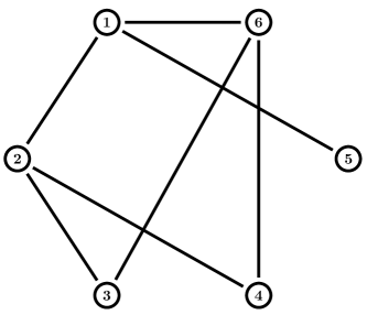
Figure 1: The leaderless communication graph.

Example 1 Consider a network of mass-spring systems with a common mass $m$ but different unknown spring constants, described by

$$m\ddot{y}_{i}+k_{i}y_{i}=u_{i},~{}i=1,\cdots,N,$$ (77)

where $y_{i}$ are the displacements from certain reference positions and $k_{i}$, $i=1,\cdots,N,$ are the bounded unknown spring constants. Denote by $x_{i}=\left[\begin{smallmatrix}y_{i}&\dot{y}_{i}\end{smallmatrix}\right]^{T}$ the state of the $i$-th agent. Then, (77) can be rewritten as

$$\dot{x}_{i}=Ax_{i}+B(u_{i}+k_{i}Ex_{i}),~{}i=1,\cdots,N,$$ (78)

with $A=\left[\begin{smallmatrix}0&1\\ 0&0\end{smallmatrix}\right]$, $B=\left[\begin{smallmatrix}0\\ \frac{1}{m}\end{smallmatrix}\right]$, $E=\left[\begin{smallmatrix}-1&0\end{smallmatrix}\right].$ It is easy to see that $k_{i}Ex_{i}$, $i=1,\cdots,N$, satisfy Assumption 2, i.e., $\|k_{i}Ex_{i}\|\leq k_{i}\|x_{i}\|$, $i=1,\cdots,N$.

Because the spring constants $k_{i}$ are unknown, we will use the adaptive protocol (23) to solve the consensus problem. Let $m=2.5kg$ and $k_{i}$ be randomly chosen. Solving the LMI (8) by using the Sedumi toolbox [33] gives the feedback gain matrices of (23) as $K=-\left[\begin{smallmatrix}0.6693&2.4595\end{smallmatrix}\right]$ and $\Gamma=\left[\begin{smallmatrix}0.4480&1.6462\\ 1.6462&6.0489\end{smallmatrix}\right].$ Assume that the communication topology is given in Fig. 1. In (23), select $\kappa=0.5$, $\varphi_{i}=\psi_{i}=0.05$, and $\tau_{i}=\epsilon_{i}=10$, $i=1,\cdots,6$, in (23). The state trajectories $x_{i}(t)$ of (78) under (23) designed as above are depicted in Fig. 2, which implies that consensus is indeed achieved. The adaptive gains $\bar{d}_{i}$ and $\bar{e}_{i}$ in (23) are shown in Fig. 3, from which it can be observed that $\bar{d}_{i}$ and $\bar{e}_{i}$ tend to be quite small.

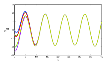
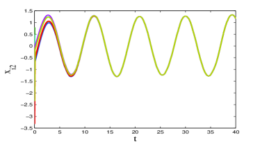
Figure 2: The state trajectories of the mass-spring systems.

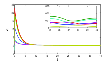
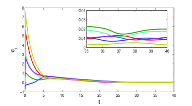
Figure 3: The adaptive gains $\bar{d}_{i}$ and $\bar{e}_{i}$ in (23).

Example 2  Consider a group of Chua’s circuits, whose dynamics in the dimensionless form are given by [34]

$$\dot{x}_{i1} =a[-x_{i1}+x_{i2}-h(x_{i1})]+u_{i},$$ (79)

$$\dot{x}_{i2} =x_{i1}-x_{i2}+x_{i3},$$

$$\dot{x}_{i2} =-bx_{i2},~{}i=0,\cdots,N,$$

where $a>0$, $b>0$, and $h(x_{i1})$ is a nonlinear function represented by $h(x_{i1})=m_{i}^{1}x_{i1}+\frac{1}{2}(m_{i}^{2}-m_{i}^{1})(|x_{i1}+1|-|x_{i1}-1|),$ where $m_{i}^{1}<0$ and $m_{i}^{2}<0$. The circuit indexed by 0 is the leader and the other circuits are the followers. It is assumed that the Chua’s circuits have nonidentical nonlinear components, i.e., $m_{i}^{1}$ and $m_{i}^{2}$ are different for different Chua’s circuits. By letting $x_{i}=[x_{i1},x_{i2},x_{i3}]^{T}$, then (79) can be rewritten in a compact form as

$$\dot{x}_{i} =Ax_{i}+B[u_{i}+f_{i}(x_{i})],~{}i=0,\cdots,N,$$ (80)

where $A=\left[\begin{smallmatrix}-m_{0}^{1}(a+1)&a&0\\ 1&-1&1\\ 0&-b&0\end{smallmatrix}\right]$, $B=\left[\begin{smallmatrix}1\\ 0\\ 0\end{smallmatrix}\right]$, $f_{0}(x_{0})=\frac{a}{2}(m_{0}^{1}-m_{0}^{2})(|x_{01}+1|-|x_{01}-1|)$, $f_{i}(x_{i})=a(m_{0}^{1}-m_{i}^{1})x_{i1}+\frac{a}{2}(m_{i}^{1}-m_{i}^{2})(|x_{i1}+1|-|x_{i1}-1|)$, $i=1,\cdots,N$. For simplicity, we let $u_{0}=0$ and take $f_{0}(x_{0})$ as the virtual control input of the leader, which clearly satisfies $\|f_{0}(x_{0})\|\leq\frac{a}{2}|m_{0}^{1}-m_{0}^{2}|$. Let $a=9$, $b=18$, $m_{0}^{1}=-\frac{3}{4}$, and $m_{0}^{2}=-\frac{4}{3}$. In this case, the leader displays a double-scroll chaotic attractor [34]. The parameters $m_{i}^{1}$ and $m_{i}^{2}$, $i=1,\cdots,N$, are randomly chosen within the interval $[-6,0)$. It is easy to see that $\|f_{i}(x_{i})\|\leq a|m_{0}^{1}-m_{i}^{1}|\|x_{i}\|+a|m_{i}^{1}-m_{i}^{2}|\\ =\frac{189}{4}\|x_{i}\|+54$, $i=1,\cdots,N.$ Note that $m_{0}^{1}$ is a parameter of the leader, which might not be available to the followers. Therefore, although $f_{i}(x_{i})$ satisfy the above condition, the upper bound of $m_{i}^{1}-m_{0}^{1}$ might be not explicitly known for the followers. Hence, we will use the adaptive protocol (55) to solve the leader-follower consensus problem.

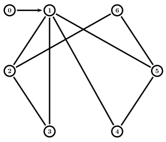
Figure 4: The leader-follower communication graph.

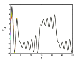
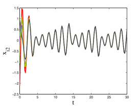
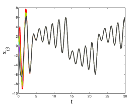
Figure 5: The state trajectories of the Chua’s circuits.

The communication graph is given as in Fig. 4, where the node indexed by 0 is the leader. Solving the LMI (8) gives the feedback gain matrices of (55) as $K=-\left[\begin{smallmatrix}16.9070&16.5791&1.8297\end{smallmatrix}\right]$ and $\Gamma=\left[\begin{smallmatrix}285.8453&280.3016&30.9344\\ 280.3016&274.8654&30.3344\\ 30.9344&30.3344&3.3477\end{smallmatrix}\right].$ To illustrate Theorem 4, select $\kappa=0.5$, $\varphi_{i}=\psi_{i}=0.05$, and $\tau_{i}=\epsilon_{i}=5$, $i=1,\cdots,6$, in (55). The state trajectories $x_{i}(t)$ of the circuits under (55) designed as above are depicted in Fig. 5, implying that leader-follower consensus is indeed achieved. The adaptive gains $\hat{d}_{i}$ and $\hat{e}_{i}$ in (55) are shown in Fig. 6, which are clearly bounded.

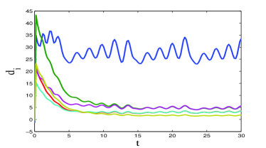
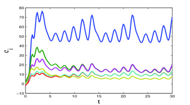
Figure 6: The adaptive gains $\hat{d}_{i}$ and $\hat{e}_{i}$ in (23).

7 Conclusion

This paper has addressed the robust consensus problem for multi-agent systems with heterogeneous matching uncertainties. For both the cases with and without a leader having a bounded unknown control input, several distributed continuous static and adaptive consensus protocols have been designed, under which the consensus error has been shown to be ultimately bounded and exponentially converges to small adjustable residual sets. It should be noted that the proposed adaptive consensus protocols can be implemented in a fully distributed fashion without requiring any global information of the communication graph or the upper bounds of the uncertainties and the leader’s control input. It has been also shown that the proposed protocols can be redesigned so as to ensure the boundedness of the consensus error in the presence of bounded external disturbances which do not necessarily satisfy the matching condition. An interesting direction for future study is to discuss the case with general directed and switching communication graphs.

References

- [1] R. Olfati-Saber, J. Fax, and R. Murray, “Consensus and cooperation in networked multi-agent systems,” Proceedings of the IEEE, vol. 95, no. 1, pp. 215–233, 2007.
- [2] W. Ren, R. Beard, and E. Atkins, “Information consensus in multivehicle cooperative control,” IEEE Control Systems Magazine, vol. 27, no. 2, pp. 71–82, 2007.
- [3] A. Jadbabaie, J. Lin, and A. Morse, “Coordination of groups of mobile autonomous agents using nearest neighbor rules,” IEEE Transactions on Automatic Control, vol. 48, no. 6, pp. 988–1001, 2003.
- [4] R. Olfati-Saber and R. Murray, “Consensus problems in networks of agents with switching topology and time-delays,” IEEE Transactions on Automatic Control, vol. 49, no. 9, pp. 1520–1533, 2004.
- [5] T. Vicsek, A. Czirók, E. Ben-Jacob, I. Cohen, and O. Shochet, “Novel type of phase transition in a system of self-driven particles,” Physical Review Letters, vol. 75, no. 6, pp. 1226–1229, 1995.
- [6] W. Ren and R. Beard, “Consensus seeking in multiagent systems under dynamically changing interaction topologies,” IEEE Transactions on Automatic Control, vol. 50, no. 5, pp. 655–661, 2005.
- [7] Y. Hong, G. Chen, and L. Bushnell, “Distributed observers design for leader-following control of multi-agent networks,” Automatica, vol. 44, no. 3, pp. 846–850, 2008.
- [8] T. Li, M. Fu, L. Xie, and J. Zhang, “Distributed consensus with limited communication data rate,” IEEE Transactions on Automatic Control, vol. 56, no. 2, pp. 279–292, 2011.
- [9] Z. Li, Z. Duan, G. Chen, and L. Huang, “Consensus of multiagent systems and synchronization of complex networks: A unified viewpoint,” IEEE Transactions on Circuits and Systems I: Regular Papers, vol. 57, no. 1, pp. 213–224, 2010.
- [10] W. Ni and D. Cheng, “Leader-following consensus of multi-agent systems under fixed and switching topologies,” Systems and Control Letters, vol. 59, no. 3-4, pp. 209–217, 2010.
- [11] H. Zhang, F. Lewis, and A. Das, “Optimal design for synchronization of cooperative systems: State feedback, observer, and output feedback,” IEEE Transactions on Automatic Control, vol. 56, no. 8, pp. 1948–1952, 2011.
- [12] K. You and L. Xie, “Network topology and communication data rate for consensusability of discrete-time multi-agent systems,” IEEE Transactions on Automatic Control, vol. 56, no. 10, pp. 2262–2275, 2011.
- [13] W. Ren, “Consensus tracking under directed interaction topologies: Algorithms and experiments,” IEEE Transactions on Control Systems Technology, vol. 18, no. 1, pp. 230–237, 2010.
- [14] Y. Cao, W. Ren, and Y. Li, “Distributed discrete-time coordinated tracking with a time-varying reference state and limited communication,” Automatica, vol. 45, no. 5, pp. 1299–1305, 2009.
- [15] W. Ren and E. Atkins, “Distributed multi-vehicle coordinated control via local information exchange,” International Journal of Robust and Nonlinear Control, vol. 17, no. 10-11, pp. 1002–1033, 2007.
- [16] F. Jiang and L. Wang, “Consensus seeking of high-order dynamic multi-agent systems with fixed and switching topologies,” International Journal of Control, vol. 85, no. 2, pp. 404–420, 2010.
- [17] R. Carli, F. Bullo, and S. Zampieri, “Quantized average consensus via dynamic coding/decoding schemes,” International Journal of Robust and Nonlinear Control, vol. 20, no. 2, pp. 156–175, 2009.
- [18] J. Mei, W. Ren, and G. Ma, “Distributed coordinated tracking with a dynamic leader for multiple Euler-Lagrange systems,” IEEE Transactions on Automatic Control, vol. 56, no. 6, pp. 1415–1421, 2011.
- [19] S. Tuna, “Conditions for synchronizability in arrays of coupled linear systems,” IEEE Transactions on Automatic Control, vol. 54, no. 10, pp. 2416–2420, 2009.
- [20] J. Seo, H. Shim, and J. Back, “Consensus of high-order linear systems using dynamic output feedback compensator: Low gain approach,” Automatica, vol. 45, no. 11, pp. 2659–2664, 2009.
- [21] C. Ma and J. Zhang, “Necessary and sufficient conditions for consensusability of linear multi-sgent systems,” IEEE Transactions on Automatic Control, vol. 55, no. 5, pp. 1263–1268, 2010.
- [22] Z. Li, W. Ren, X. Liu, and M. Fu, “Consensus of multi-agent systems with general linear and Lipschitz nonlinear dynamics using distributed adaptive protocols,” IEEE Transactions on Automatic Control, in press, 2013.
- [23] Z. Li, W. Ren, X. Liu, and L. Xie, “Distributed consensus of linear multi-agent systems with adaptive dynamic protocols,” Automatica, in press, 2013.
- [24] Z. Li, X. Liu, W. Ren, and L. Xie, “Distributed tracking control for linear multi-agent systems with a leader of bounded unknown input,” IEEE Transactions on Automatic Control, vol. 58, no. 2, pp. 518–523, 2013.
- [25] A. Das and F. L. Lewis, “Distributed adaptive control for synchronization of unknown nonlinear networked systems,” Automatica, vol. 46, no. 12, pp. 2014–2021, 2010.
- [26] H. Zhang and F. Lewis, “Adaptive cooperative tracking control of higher-order nonlinear systems with unknown dynamics,” Automatica, vol. 48, no. 7, pp. 1432–1439, 2012.
- [27] G. Wheeler, C. Su, and Y. Stepanenko, “A sliding mode controller with improved adaptation laws for the upper bounds on the norm of uncertainties,” Automatica, vol. 34, no. 12, pp. 1657–1661, 1998.
- [28] C. Edwards and S. Spurgeon, Sliding Mode Control: Theory and Applications. London: Taylor & Francis, 1998.
- [29] Z. Li, Z. Duan, and G. Chen, “Dynamic consensus of linear multi-agent systems,” IET Control Theory and Applications, vol. 5, no. 1, pp. 19–28, 2011.
- [30] H. Khalil, Nonlinear Systems. Englewood Cliffs, NJ: Prentice Hall, 2002.
- [31] K. Young, V. Utkin, and U. Ozguner, “A control engineer’s guide to sliding mode control,” IEEE Transactions on Control Systems Technology, vol. 7, no. 3, pp. 328–342, 1999.
- [32] P. Ioannou and P. Kokotovic, “Instability analysis and improvement of robustness of adaptive control,” Automatica, vol. 20, no. 5, pp. 583–594, 1984.
- [33] J. Sturm, “Using SeDuMi 1.02, a MATLAB toolbox for optimization over symmetric cones,” Optimization Methods and Software, vol. 11, no. 1, pp. 625–653, 1999.
- [34] R. Madan, Chua’s circuit: a paradigm for chaos. Singapore: World Scientific, 1993.