Designing Fully Distributed Consensus Protocols for Linear Multi-agent Systems with Directed Graphs

Abstract

This technical note addresses the distributed consensus protocol design problem for multi-agent systems with general linear dynamics and directed communication graphs. Existing works usually design consensus protocols using the smallest real part of the nonzero eigenvalues of the Laplacian matrix associated with the communication graph, which however is global information. In this technical note, based on only the agent dynamics and the relative states of neighboring agents, a distributed adaptive consensus protocol is designed to achieve leader-follower consensus in the presence of a leader with a zero input for any communication graph containing a directed spanning tree with the leader as the root node. The proposed adaptive protocol is independent of any global information of the communication graph and thereby is fully distributed. Extensions to the case with multiple leaders are further studied.

I Introduction

Consensus of multi-agent systems has been an emerging research topic in the systems and control community in recent years. Due to its potential applications in several areas such as spacecraft formation flying, sensor networks, and cooperative surveillance [1], the consensus control problem has been addressed by many researchers from various perspectives; see [1, 2, 3, 4, 5] and the references therein. Existing consensus algorithms can be roughly categorized into two classes, namely, consensus without a leader (i.e., leaderless consensus) and consensus with a leader which is also called leader-follower consensus or distributed tracking. For the consensus control problem, a key task is to design appropriate distributed controllers which are usually called consensus protocols. Due to the spatial distribution of the agents and limited sensing capability of sensors, implementable consensus protocols for multi-agent systems should be distributed, depending on only the local state or output information of each agent and its neighbors.

In this technical note, we consider the distributed consensus protocol design problem for multi-agent systems with general continuous-time linear dynamics. Previous works along this line include [6, 7, 8, 9, 10, 11], where different static and dynamic consensus protocols have been proposed. One common feature in the aforementioned works is that the design of the consensus protocols requires the knowledge of some eigenvalue information of the Laplacian matrix associated with the communication graph (specifically, the smallest nonzero eigenvalue of the Laplacian matrix for undirected graphs and the smallest real part of the nonzero eigenvalues of the Laplacian matrix for directed graphs). As pointed in [8], for the case where the agents are not neutrally stable, e.g., double integrators, the design of the consensus protocols generally depends on the smallest real part of the nonzero eigenvalues of the Laplacian matrix. However, it is worth mentioning that the smallest real part of the nonzero eigenvalues of the Laplacian matrix is global information in the sense that each agent has to know the entire communication graph $\mathcal{G}$ to compute it. Therefore, the consensus protocols given in the aforementioned papers cannot be designed by each agent in a fully distributed fashion, i.e., using only the local information of its own and neighbors. To overcome this limitation, distributed adaptive consensus protocols are proposed in [12, 13]. Similar adaptive schemes are presented to achieve second-order consensus with nonlinear dynamics in [14, 15]. Note that the protocols in [12, 13, 14, 15] are applicable to only undirected communication graphs or leader-follower graphs where the subgraphs among the followers are undirected. How to design fully distributed adaptive consensus protocols for the case with general directed graphs is quite challenging and to the best of our knowledge is still open. The main difficulty lies in that the Laplacian matrices of directed graphs are generally asymmetric, which renders the construction of adaptive consensus protocol and the selection of appropriate Lyapunov function far from being easy.

In this technical note, we intend to design fully distributed consensus protocols for general linear multi-agent systems with a leader of a zero input and a directed communication graph. Based on the relative states of neighboring agents, a distributed adaptive consensus protocol is constructed. It is shown via a novel Lyapunov function that the proposed adaptive protocol can achieve leader-follower consensus for any communication graph containing a directed spanning tree with the leader as the root node. The adaptive protocol proposed in this technical note, independent of any global information of the communication graph, relies on only the agent dynamics and the relative state information and thereby is fully distributed. Compared to the distributed adaptive protocols in [12, 13] for undirected graphs, a distinct feature of the adaptive protocol in this technical note is that monotonically increasing functions, inspired by the changing supply function notion in [16], are introduced to provide extra freedom for design. As an extension, we consider the case where there exist multiple leaders with zero inputs. In this case, it is shown that the proposed adaptive protocol can solve the containment control problem, i.e., the states of the followers are to be driven into the convex hull spanned by the states of the leaders, if for each follower, there exists at least one leader that has a directed path to that follower. A sufficient condition for the existence of the adaptive protocol in this technical note is that each agent is stabilizable.

The rest of this technical note is organized as follows. Mathematical preliminaries required in this paper are summarized in Section II. The problem is formulated and the motivation is stated in Section III. Distributed adaptive consensus protocols are designed in Section IV for general directed leader-follower graphs. Extensions to the case with multiple leaders are studied in Section V. Simulation examples are presented for illustration in Section VI. Conclusions are drawn in Section VII.

II Mathematical Preliminaries

Throughout this technical note, the following notations and definitions will be used: $\mathbf{R}^{n\times m}$ and $\mathbf{C}^{n\times m}$ denote the sets of $n\times m$ real and complex matrices, respectively. $I_{N}$ represents the identity matrix of dimension $N$. Denote by $\mathbf{1}$ a column vector with all entries equal to one. ${\mathrm{diag}}(A_{1},\cdots,A_{n})$ represents a block-diagonal matrix with matrices $A_{i},i=1,\cdots,n,$ on its diagonal. For real symmetric matrices $X$ and $Y$, $X>(\geq)Y$ means that $X-Y$ is positive (semi-)definite. For a vector $x$, $x>(\geq)0$ means that every entry of $x$ is positive (nonnegative). $A\otimes B$ denotes the Kronecker product of matrices $A$ and $B$. ${\mathrm{Re}}(\alpha)$ represents the real part of $\alpha\in\mathbf{C}$. A matrix $A=[a_{ij}]\in\mathbf{R}^{n\times n}$ is called a nonsingular $M$-matrix, if $a_{ij}<0$, $\forall i\neq j$, and all eigenvalues of $A$ have positive real parts.

A directed graph $\mathcal{G}$ is a pair $(\mathcal{V},\mathcal{E})$, where $\mathcal{V}=\{v_{1},\cdots,v_{N}\}$ is a nonempty finite set of nodes and $\mathcal{E}\subseteq\mathcal{V}\times\mathcal{V}$ is a set of edges, in which an edge is represented by an ordered pair of distinct nodes. For an edge $(v_{i},v_{j})$, node $v_{i}$ is called the parent node, node $v_{j}$ the child node, and $v_{i}$ is a neighbor of $v_{j}$. A graph with the property that $(v_{i},v_{j})\in\mathcal{E}$ implies $(v_{j},v_{i})\in\mathcal{E}$ for any $v_{i},v_{j}\in\mathcal{V}$ is said to be undirected. A path from node $v_{i_{1}}$ to node $v_{i_{l}}$ is a sequence of ordered edges of the form $(v_{i_{k}},v_{i_{k+1}})$, $k=1,\cdots,l-1$. A directed graph contains a directed spanning tree if there exists a node called the root, which has no parent node, such that the node has directed paths to all other nodes in the graph.

The adjacency matrix $\mathcal{A}=[a_{ij}]\in\mathbf{R}^{N\times N}$ associated with the directed graph $\mathcal{G}$ is defined by $a_{ii}=0$, $a_{ij}$ is a positive value if $(v_{j},v_{i})\in\mathcal{E}$ and $a_{ij}=0$ otherwise. Note that $a_{ij}$ denotes the weight for the edge $(v_{j},v_{i})\in\mathcal{E}$. If the weights are not relevant, then $a_{ij}$ is set equal to 1 if $(v_{j},v_{i})\in\mathcal{E}$. The Laplacian matrix $\mathcal{L}=[\mathcal{L}_{ij}]\in\mathbf{R}^{N\times N}$ is defined as $\mathcal{L}_{ii}=\sum_{j\neq i}a_{ij}$ and $\mathcal{L}_{ij}=-a_{ij}$, $i\neq j$.

Lemma 1 ([17])

Zero is an eigenvalue of $\mathcal{L}$ with $\mathbf{1}$ as a right eigenvector and all nonzero eigenvalues have positive real parts. Furthermore, zero is a simple eigenvalue of $\mathcal{L}$ if and only if $\mathcal{G}$ has a directed spanning tree.

Lemma 2 (Young’s Inequality, [18])

If $a$ and $b$ are nonnegative real numbers and $p$ and $q$ are positive real numbers such that $1/p+1/q=1$, then $ab\leq\frac{a^{p}}{p}+\frac{b^{q}}{q}$.

III Problem Statement and Motivations

Consider a group of $N+1$ identical agents with general linear dynamics, consisting of $N$ followers and a leader. The dynamics of the $i$-th agent are described by

$$\dot{x}_{i} =Ax_{i}+Bu_{i},\quad i=0,\cdots,N,$$ (1)

where $x_{i}\in\mathbf{R}^{n}$ is the state, $u_{i}\in\mathbf{R}^{p}$ is the control input, and $A$ and $B$ are constant matrices with compatible dimensions.

Without loss of generality, let the agent in (1) indexed by 0 be the leader (which receives no information from any follower) and the agents indexed by $1,\cdots,N$, be the followers. It is assumed that the leader’s control input is zero, i.e., $u_{0}=0$. The communication graph $\mathcal{G}$ among the $N+1$ agents is assumed to satisfy the following assumption.

Assumption 1: The graph $\mathcal{G}$ contains a directed spanning tree with the leader as the root node .

Denote by $\mathcal{L}$ the Laplacian matrix associated with $\mathcal{G}$. Because the node indexed by 0 is the leader which has no neighbors, $\mathcal{L}$ can be partitioned as

$$\mathcal{L}=\begin{bmatrix}0&0_{1\times N}\\ \mathcal{L}_{2}&\mathcal{L}_{1}\end{bmatrix},$$ (2)

where $\mathcal{L}_{2}\in\mathbf{R}^{N\times 1}$ and $\mathcal{L}_{1}\in\mathbf{R}^{N\times N}$. Since $\mathcal{G}$ satisfies Assumption 1, it follows from Lemma 1 that all eigenvalues of $\mathcal{L}_{1}$ have positive real parts. It then can be verified that $\mathcal{L}_{1}$ is a nonsingular $M$-matrix and is diagonally dominant.

The intention of this technical note is to solve the leader-follower consensus problem for the agent in (1), i.e., to design distributed consensus protocols under which the states of the $N$ followers converge to the state of the leader in the sense of $\lim_{t\rightarrow\infty}\|x_{i}(t)-x_{0}(t)\|=0$, $\forall\,i=1,\cdots,N.$

Several consensus protocols have been proposed to reach leader-follower consensus for the agents in (1), e.g., in [6, 7, 9, 23, 8, 10]. A static consensus protocol based on the relative states between neighboring agents is given in [6, 10] as

$$u_{i}=c\tilde{K}\sum_{j=1}^{N}a_{ij}(x_{i}-x_{j}),\quad i=1,\cdots,N,$$ (3)

where $c>0$ is the common coupling weight among neighboring agents, $\tilde{K}\in\mathbf{R}^{p\times n}$ is the feedback gain matrix, and $a_{ij}$ is $(i,j)$-th entry of the adjacency matrix $\mathcal{A}$ associated with $\mathcal{G}$.

Lemma 3 ([6, 10])

For the communication graph $\mathcal{G}$ satisfying Assumption 1, the $N$ agents described by (1) reach leader-follower consensus under the protocol (3) with $\tilde{K}=-B^{T}P^{-1}$ and $c\geq 1/\underset{i=1,\cdot\cdot,N}{\min}\mathrm{Re}(\lambda_{i})$, where $\lambda_{i}$, $i=1,\cdots,N$, are the nonzero eigenvalues of $\mathcal{L}_{1}$ and $P>0$ is a solution to the following linear matrix inequality (LMI):

$$AP+PA^{T}-2BB^{T}<0.$$ (4)

As shown in the above lemma, in order to reach consensus, the coupling weight $c$ should be not less than the inverse of $\underset{i=1,\cdot\cdot,N}{\min}\mathrm{Re}(\lambda_{i})$, that is, the smallest real part of the eigenvalues of $\mathcal{L}_{1}$. Actually it is pointed out in [8, 23] that for the case where the agents in (1) are critically unstable, e.g., double integrators, the design of the consensus protocol generally requires the knowledge of $\underset{i=1,\cdot\cdot,N}{\min}\mathrm{Re}(\lambda_{i})$. However, it is worth mentioning that $\underset{i=1,\cdot\cdot,N}{\min}\mathrm{Re}(\lambda_{i})$ is global information in the sense that each follower has to know the entire communication graph $\mathcal{G}$ to compute it. Therefore, the consensus protocols given in Lemma 3 cannot be designed by each agent in a fully distributed fashion, i.e., using only the local information of its own and neighbors. This limitation motivates us to design some fully distributed consensus protocols for the agents in (1) whose directed communication graph satisfies Assumption 1.

IV Distributed Adaptive Consensus Protocol Design

In this section, we consider the case where each agent has access to the relative states of its neighbors with respect to itself. Based on the relative states of neighboring agents, we propose the following distributed adaptive consensus protocol with time-varying coupling weights:

$$u_{i} =c_{i}\rho_{i}(\xi_{i}^{T}P^{-1}\xi_{i})K\xi_{i},$$ (5)

$$\dot{c}_{i} =\xi_{i}^{T}\Gamma\xi_{i},\quad i=1,\cdots,N,$$

where $\xi_{i}\triangleq\sum_{j=0}^{N}a_{ij}(x_{i}-x_{j})$, $c_{i}(t)$ denotes the time-varying coupling weight associated with the $i$-th follower with $c_{i}(0)\geq 1$, $P>0$ is a solution to the LMI (4), $K\in\mathbf{R}^{p\times n}$ and $\Gamma\in\mathbf{R}^{n\times n}$ are the feedback gain matrices to be designed, $\rho_{i}(\cdot)$ are smooth and monotonically increasing functions to be determined later which satisfies that $\rho_{i}(s)\geq 1$ for $s>0$, and the rest of variables are defined as in (3).

Let $\xi=[\xi_{1}^{T},\cdots,\xi_{N}^{T}]^{T}$. Then,

$$\xi=(\mathcal{L}_{1}\otimes I_{n})\begin{bmatrix}x_{1}-x_{0}\\ \vdots\\ x_{N}-x_{0}\end{bmatrix},$$ (6)

where $\mathcal{L}_{1}$ is defined in (2). Because $\mathcal{L}_{1}$ is nonsingular for $\mathcal{G}$ satisfying Assumption 1, it is easy to see that the leader-follower consensus problem is solved if and only if $\xi$ asymptotically converges to zero. Hereafter, we refer to $\xi$ as the consensus error. In light of (1) and (5), it is not difficult to obtain that $\xi$ and $c_{i}$ satisfy the following dynamics:

$$\dot{\xi} =[I_{N}\otimes A+\mathcal{L}_{1}\widehat{C}\hat{\rho}(\xi)\otimes BK]\xi,$$ (7)

$$\dot{c}_{i} =\xi_{i}^{T}\Gamma\xi_{i},$$

where $\hat{\rho}(\xi)\triangleq{\mathrm{diag}}(\rho_{1}(\xi_{1}^{T}P^{-1}\xi_{1}),\cdots,\rho_{N}(\xi_{N}^{T}P^{-1}\xi_{N}))$ and $\widehat{C}\triangleq{\mathrm{diag}}(c_{1},\cdots,c_{N})$.

Before moving on to present the main result of this section, we first introduce a property of the nonsingular $M$-matrix $\mathcal{L}_{1}$.

Lemma 4

There exists a positive diagonal matrix $G$ such that $G\mathcal{L}_{1}+\mathcal{L}_{1}^{T}G>0$. One such $G$ is given by ${\mathrm{diag}}(q_{1},\cdots,q_{N})$, where $q=[q_{1},\cdots,q_{N}]^{T}=(\mathcal{L}_{1}^{T})^{-1}{\bf 1}$.

Proof:

The first assertion is well known; see Theorem 4.25 in [19] or Theorem 2.3 in [20]. The second assertion is shown in the following. Note that the specific form of $G$ given here is different from that in [19, 21, 22].

Since $\mathcal{L}_{1}$ is a nonsingular $M$-matrix, it follows from Theorem 4.25 in [19] that $(\mathcal{L}_{1}^{T})^{-1}$ exists, is nonnegative, and thereby cannot have a zero row. Then, it is easy to verify that $q>0$ and hence $G\mathcal{L}_{1}{\bf 1}\geq 0$. By noting that $\mathcal{L}_{1}^{T}G{\bf 1}=\mathcal{L}_{1}^{T}q={\bf 1}$, we can conclude that $(G\mathcal{L}_{1}+\mathcal{L}_{1}^{T}G){\bf 1}>0$, implying that $G\mathcal{L}_{1}+\mathcal{L}_{1}^{T}G$ is strictly diagonally dominant. Since the diagonal entries of $G\mathcal{L}_{1}+\mathcal{L}_{1}^{T}G$ are positive, it then follows from Gershgorin’s disc theorem [18] that every eigenvalue of $G\mathcal{L}_{1}+\mathcal{L}_{1}^{T}G$ is positive, implying that $G\mathcal{L}_{1}+\mathcal{L}_{1}^{T}G>0$. ∎

The following result provides a sufficient condition to design the adaptive consensus protocol (5).

Theorem 1

Suppose that the communication graph $\mathcal{G}$ satisfies Assumption 1. Then, the leader-follower consensus problem of the agents in (1) is solved by the adaptive protocol (5) with $K=-B^{T}P^{-1}$, $\Gamma=P^{-1}BB^{T}P^{-1}$, and $\rho_{i}(\xi_{i}^{T}P^{-1}\xi_{i})=(1+\xi_{i}^{T}P^{-1}\xi_{i})^{3}$, where $P>0$ is a solution to the LMI (4). Moreover, each coupling weight $c_{i}$ converges to some finite steady-state value.

Proof:

Consider the following Lyapunov function candidate:

$$V_{1}=\sum_{i=1}^{N}\frac{c_{i}q_{i}}{2}\int_{0}^{\xi_{i}^{T}P^{-1}\xi_{i}}\rho_{i}(s)ds+\frac{\hat{\lambda}_{0}}{24}\sum_{i=1}^{N}\tilde{c}_{i}^{2},$$ (8)

where $\tilde{c}_{i}=c_{i}-\alpha$, $\alpha$ is a positive scalar to be determined later, $\hat{\lambda}_{0}$ denotes the smallest eigenvalue of $G\mathcal{L}_{1}+\mathcal{L}_{1}^{T}G$, and $G\triangleq{\mathrm{diag}}(q_{1},\cdots,q_{N})$ is chosen as in Lemma 4 such that $G\mathcal{L}_{1}+\mathcal{L}_{1}^{T}G>0$. Because $c_{i}(0)\geq 1$, it follows from the second equation in (7) that $c_{i}(t)\geq 1$ for $t>0$. Furthermore, by noting that $\rho_{i}(\cdot)$ are smooth and monotonically increasing functions satisfying $\rho_{i}(s)\geq 1$ for $s>0$, it is not difficult to see that $V_{1}$ is positive definite with respect to $\xi_{i}$ and $\tilde{c}_{i}$, $i=1,\cdots,N$.

The time derivative of $V_{1}$ along the trajectory of (7) is given by

$$\dot{V}_{1} =\sum_{i=1}^{N}c_{i}q_{i}\rho_{i}(\xi_{i}^{T}P^{-1}\xi_{i})\xi_{i}^{T}P^{-1}\dot{\xi}_{i}$$ (9)

$$\quad+\sum_{i=1}^{N}\frac{\dot{c}_{i}q_{i}}{2}\int_{0}^{\xi_{i}^{T}P^{-1}\xi_{i}}\rho_{i}(s)ds$$

$$\quad+\frac{\hat{\lambda}_{0}}{12}\sum_{i=1}^{N}(c_{i}-\alpha)\xi_{i}^{T}P^{-1}BB^{T}P^{-1}\xi_{i}.$$

In the sequel, for conciseness we shall use $\hat{\rho}$ and $\rho_{i}$ instead of $\hat{\rho}(\xi)$ and $\rho_{i}(\xi_{i}^{T}P^{-1}\xi_{i})$, respectively, whenever without causing any confusion.

By using (7) and after some mathematical manipulations, we can get that

$$\sum_{i=1}^{N}c_{i}q_{i}\rho_{i}\xi_{i}^{T}P^{-1}\dot{\xi}_{i} =\xi^{T}(\widehat{C}\hat{\rho}G\otimes P^{-1})\dot{\xi}$$ (10)

$$=\frac{1}{2}\xi^{T}[\widehat{C}\hat{\rho}G\otimes(P^{-1}A+A^{T}P^{-1})$$

$$\quad-\widehat{C}\hat{\rho}(G\mathcal{L}_{1}+\mathcal{L}_{1}^{T}G)\widehat{C}\hat{\rho}\otimes P^{-1}BB^{T}P^{-1}]\xi$$

$$\leq\frac{1}{2}\xi^{T}[\widehat{C}\hat{\rho}G\otimes(P^{-1}A+A^{T}P^{-1})$$

$$\quad-\hat{\lambda}_{0}\widehat{C}^{2}\hat{\rho}^{2}\otimes P^{-1}BB^{T}P^{-1}]\xi,$$

where we have used the fact that $G\mathcal{L}_{1}+\mathcal{L}_{1}^{T}G\geq\hat{\lambda}_{0}I$ to get the first inequality.

Because $\rho_{i}$ are monotonically increasing and satisfy $\rho_{i}(s)\geq 1$ for $s>0$, it follows that

$$\sum_{i=1}^{N}\dot{c}_{i}q_{i}\int_{0}^{\xi_{i}^{T}P^{-1}\xi_{i}}\rho_{i}(s)ds \leq\sum_{i=1}^{N}\dot{c}_{i}q_{i}\rho_{i}\xi_{i}^{T}P^{-1}\xi_{i}$$ (11)

$$\leq\sum_{i=1}^{N}\frac{\dot{c}_{i}q_{i}^{3}}{3\hat{\lambda}_{0}^{2}}+\sum_{i=1}^{N}\frac{2}{3}\hat{\lambda}_{0}\dot{c}_{i}\rho_{i}^{\frac{3}{2}}(\xi_{i}^{T}P^{-1}\xi_{i})^{\frac{3}{2}}$$

$$\leq\sum_{i=1}^{N}\frac{\dot{c}_{i}q_{i}^{3}}{3\hat{\lambda}_{0}^{2}}+\sum_{i=1}^{N}\frac{2}{3}\hat{\lambda}_{0}\dot{c}_{i}\rho_{i}^{\frac{3}{2}}(1+\xi_{i}^{T}P^{-1}\xi_{i})^{\frac{3}{2}}$$

$$=\sum_{i=1}^{N}(\frac{q_{i}^{3}}{3\hat{\lambda}_{0}^{2}}+\frac{2}{3}\hat{\lambda}_{0}\rho_{i}^{2})\xi_{i}^{T}P^{-1}BB^{T}P^{-1}\xi_{i},$$

where we have used the mean value theorem for integrals to get the first inequality and used Lemma 2 to get the second inequality.

Substituting (10) and (11) into (9) yields

$$\dot{V}_{1} \leq\frac{1}{2}\xi^{T}[\widehat{C}\hat{\rho}G\otimes(P^{-1}A+A^{T}P^{-1})]\xi$$ (12)

$$\quad-\sum_{i=1}^{N}[\hat{\lambda}_{0}(\frac{1}{2}c_{i}^{2}\rho_{i}^{2}-\frac{1}{12}c_{i}-\frac{1}{3}\rho_{i}^{2})$$

$$\quad+\frac{1}{12}(\hat{\lambda}_{0}\alpha-\frac{2q_{i}^{3}}{\hat{\lambda}_{0}^{2}})]\xi^{T}_{i}P^{-1}BB^{T}P^{-1}\xi_{i}.$$

Choose $\alpha\geq\hat{\alpha}+\max_{i=1,\cdots,N}\frac{2q_{i}^{3}}{\hat{\lambda}_{0}^{3}}$, where $\hat{\alpha}>0$ will be determined later. Then, by noting that $\rho_{i}\geq 1$ and $c_{i}\geq 1$, $i=1,\cdots,N$, it follows from (12) that

$$\dot{V}_{1} \leq\frac{1}{2}\xi^{T}[\widehat{C}\hat{\rho}G\otimes(P^{-1}A+A^{T}P^{-1})]\xi$$ (13)

$$\quad-\frac{\hat{\lambda}_{0}}{12}\sum_{i=1}^{N}(c_{i}^{2}\rho_{i}^{2}+\hat{\alpha})\xi^{T}_{i}P^{-1}BB^{T}P^{-1}\xi_{i}$$

$$\leq\frac{1}{2}\xi^{T}[\widehat{C}\hat{\rho}G\otimes(P^{-1}A+A^{T}P^{-1})$$

$$\quad-\frac{1}{3}\sqrt{\hat{\alpha}}\hat{\lambda}_{0}\widehat{C}\hat{\rho}\otimes P^{-1}BB^{T}P^{-1}]\xi.$$

Let $\tilde{\xi}=(\sqrt{\widehat{C}\hat{\rho}G}\otimes I)\xi$ and choose $\hat{\alpha}$ to be sufficiently large such that $\sqrt{\hat{\alpha}}\hat{\lambda}_{0}G^{-1}\geq 6I$. Then, we can get from (13) that

$$\dot{V}_{1} \leq\frac{1}{2}\tilde{\xi}^{T}[I_{N}\otimes(P^{-1}A+A^{T}P^{-1}-2P^{-1}BB^{T}P^{-1})]\tilde{\xi}$$ (14)

$$\leq 0,$$

where to get the last inequality we have used the assertion that $P^{-1}A+A^{T}P^{-1}-2P^{-1}BB^{T}P^{-1}<0$, which follows readily from (4).

Since $\dot{V}_{1}\leq 0$, $V_{1}(t)$ is bounded and so is each $c_{i}$. By noting $\dot{c}_{i}\geq 0$, it can be seen from (7) that $c_{i}$ are monotonically increasing. Then, it follows that each coupling weight $c_{i}$ converges to some finite value. Note that $\dot{V}_{1}\equiv 0$ implies that $\tilde{\xi}=0$ and thereby $\xi=0$. Hence, by LaSalle’s Invariance principle [24], it follows that the consensus error $\xi$ asymptotically converges to zero. That is, the leader-follower consensus problem is solved. ∎

Remark 1

As shown in [6], a necessary and sufficient condition for the existence of a $P>0$ to the LMI (4) is that $(A,B)$ is stabilizable. Therefore, a sufficient condition for the existence of an adaptive protocol (5) satisfying Theorem 1 is that $(A,B)$ is stabilizable. The consensus protocol (5) can also be designed by solving the algebraic Ricatti equation: $A^{T}Q+QA+I-QBB^{T}Q=0$, as in [23, 10]. In this case, the parameters in (5) can be chosen as $K=-B^{T}Q$, $\Gamma=QBB^{T}Q$, and $\rho_{i}=(1+\xi_{i}^{T}Q\xi_{i})^{3}$. The solvability of the above Ricatti equation is equal to that of the LMI (4).

Remark 2

In contrast to the consensus protocols in [6, 7, 9, 23, 10] which require the knowledge of the eigenvalues of the asymmetric Laplacian matrix, the adaptive protocol (5) depends on only the agent dynamics and the relative states of neighboring agents, and thereby can be computed and implemented by each agent in a fully distributed way. Compared to the adaptive protocols in [13, 12] which are applicable to only undirected graphs or leader-follower graphs where the subgraph among the followers is undirected, the adaptive consensus protocol (5) works for general directed leader-follower communication graphs.

Remark 3

In comparison to the adaptive protocols in [13, 12], a distinct feature of (5) is that inspired by the changing supply functions in [16], monotonically increasing functions $\rho_{i}$ are introduced into (5) to provide extra freedom for design. As the consensus error $\xi$ converges to zero, the functions $\rho_{i}$ will converge to 1, in which case the adaptive protocol (5) will reduce to the adaptive protocols for undirected graphs in [13, 12]. It is worth mentioning that the Lyapunov function used in the proof of Theorem 1 is partly motivated by [25] which designs adaptive consensus protocols for first-order multi-agent systems with uncertainties.

V Extensions to The Case with Multiple Leaders

In this section, we extend to consider the case where there exist more than one leader. In the presence of multiple leaders, the containment control problem arises, where the states of the followers are to be driven into the convex hull spanned by those of the leaders [26].

The dynamics of the $N+1$ agents are still described by (1). Without loss of generality, the agents indexed by $0,\cdots,M$ ($M<N-1$), are the leaders whose control inputs are assumed to be zero and the agents indexed by $M+1,\cdots,N$, are the followers. The communication graph $\mathcal{G}$ among the $N+1$ agents is assumed to satisfy the following assumption.

Assumption 2: For each follower, there exists at least one leader that has a directed path to that follower.

Clearly, Assumption 2 will reduce to Assumption 1 if only one leader exists. Under Assumption 2, the Laplacian matrix $\mathcal{L}$ can be written as $\mathcal{L}=\begin{bmatrix}0_{(M+1)\times(M+1)}&0_{(M+1)\times(N-M)}\\ \widetilde{\mathcal{L}}_{2}&\widetilde{\mathcal{L}}_{1}\\ \end{bmatrix},$ where $\widetilde{\mathcal{L}}_{1}\in\mathbf{R}^{(N-M)\times(N-M)}$, $\widetilde{\mathcal{L}}_{2}\in\mathbf{R}^{(M+1)\times(N-M)}$, and the following result holds.

Lemma 5

[26] Under Assumption 2, all the eigenvalues of $\widetilde{\mathcal{L}}_{1}$ have positive real parts, each entry of $-\widetilde{\mathcal{L}}_{1}^{-1}\widetilde{\mathcal{L}}_{2}$ is nonnegative, and each row of $-\widetilde{\mathcal{L}}_{1}^{-1}\widetilde{\mathcal{L}}_{2}$ has a sum equal to one.

In the following, we will investigate if the proposed adaptive protocol (5) can solve the containment control problem for the case where $\mathcal{G}$ satisfies Assumption 2. In this case, $\zeta\triangleq[\xi_{M+1}^{T},\cdots,\xi_{M+1}^{T}]^{T}$, where $\xi_{i}$ is defined in (5), can be written into

$$\zeta=(\widetilde{\mathcal{L}}_{2}\otimes I_{n})\begin{bmatrix}x_{0}\\ \vdots\\ x_{M}\end{bmatrix}+(\widetilde{\mathcal{L}}_{1}\otimes I_{n})\begin{bmatrix}x_{M+1}\\ \vdots\\ x_{N}\end{bmatrix}.$$ (15)

Clearly, $\zeta=0$ if and only if $\begin{bmatrix}x_{M+1}\\ \vdots\\ x_{N}\end{bmatrix}=-(\widetilde{\mathcal{L}}_{1}^{-1}\widetilde{\mathcal{L}}_{2}\otimes I_{n})\begin{bmatrix}x_{0}\\ \vdots\\ x_{M}\end{bmatrix}$, which, in light of Lemma 5, implies that the states of the followers $x_{i}$, $i=M+1,\cdots,N,$ lie within the convex hull spanned by the states of the leaders. Thus, the containment control problem can be reduced to the asymptotical stability of $\zeta$. By using (1), (5), and (15), we can obtain that $\zeta$ and $c_{i}$ satisfy

$$\dot{\zeta} =[I_{N-M}\otimes A+\widetilde{\mathcal{L}}_{1}\widetilde{C}\tilde{\rho}(\zeta)\otimes BK]\zeta,$$

$$\dot{c}_{i} =\xi_{i}^{T}\Gamma\xi_{i},\quad i=M+1,\cdots,N,$$

where $\tilde{\rho}(\zeta)\triangleq{\mathrm{diag}}(\rho_{M+1}(\xi_{M+1}^{T}P^{-1}\xi_{M+1}),\cdots,\rho_{N}(\xi_{N}^{T}P^{-1}\xi_{N}))$ and $\widetilde{C}\triangleq{\mathrm{diag}}(c_{M+1},\cdots,c_{N})$.

The following theorem can be shown by following similar steps in proving Theorem 1.

Theorem 2

Supposing that $\mathcal{G}$ satisfies Assumption 2, the adaptive protocol (5) designed as in Theorem 1 can solve the containment control problem for the agents in (1) and each coupling weight $c_{i}$ converges to some finite steady-state value.

Remark 4

Theorem 2 extends Theorem 1 to the case with multiple leaders. For the case with only one leader, Theorem 2 will reduce to Theorem 1. The containment control problem of general linear multi-agent systems was previously discussed in [27]. Contrary to the static controller in [27] whose design relies on the smallest real part of the eigenvalues of $\widetilde{\mathcal{L}}_{1}$, the adaptive protocol (5) depends on only local information and thus is fully distributed.

VI Simulation Example

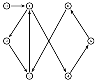
Figure 1: The directed communication graph.

In this section, a simulation example is provided for illustration.

Consider a network of third-order integrators, described by (1), with

$$A=\left[\begin{matrix}0&1&0\\ 0&0&1\\ 0&0&0\end{matrix}\right],\quad B=\left[\begin{matrix}0\\ 0\\ 1\end{matrix}\right].$$

The communication graph is given as in Fig. 1, where the node indexed by 0 is the leader which is only accessible to the node indexed by 1. The weights of the graph are randomly chosen within the interval $(0,3)$. It is easy to verify that the graph in Fig. 1 satisfies Assumption 1.

Solving the LMI (4) by using the SeDuMi toolbox [28] gives a solution

$$P=\begin{bmatrix}3.0861&-0.6245&-0.5186\\ -0.6245&1.1602&-0.5573\\ -0.5186&-0.5573&0.9850\end{bmatrix}.$$

Thus, the feedback gain matrices in (5) are obtained as

$$K =-\begin{bmatrix}0.6285&1.3525&2.1113\end{bmatrix},$$

$$\Gamma =\begin{bmatrix}0.3950&0.8500&1.3269\\ 0.8500&1.8292&2.8554\\ 1.3269&2.8554&4.4574\end{bmatrix}.$$

To illustrate Theorem 1, let the initial states $c_{i}(0)$ and $\rho_{i}(0)$ be randomly chosen within the interval $[1,3]$. The consensus errors $x_{i}-x_{0}$, $i=1,\cdots,6$, of the double integrators, under the adaptive protocol (5) with $K$, $\Gamma$, and $\rho_{i}$ chosen as in Theorem 1, are depicted in in Fig. 2, which states that leader-follower consensus is indeed achieved. The coupling weights $c_{i}$ associated with the followers are drawn in Fig. 3, from which it can be observed that the coupling weights converge to finite steady-state values.

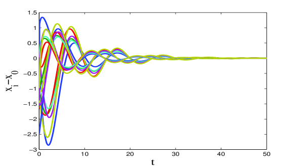
Figure 2: $x_{i}-x_{0}$, $i=1,\cdots,6$, of third-order integrators under the adaptive protocol (5).

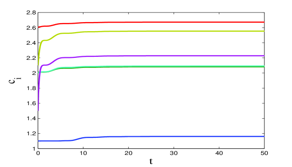
Figure 3: The adaptive coupling gains $c_{i}$ in (5).

VII Conclusion

In this technical note, we have addressed the distributed consensus problem for a multi-agent system with general linear dynamics and a directed leader-follower communication graph. The main contribution of this technical note is that for any communication graph containing a directed spanning tree with the leader as the root, a distributed adaptive consensus protocol is designed, which, depending on only the agent dynamics and the relative state information of neighboring agents, is fully distributed. The case with multiple leaders has been also discussed.

It is worth mentioning that in this technical note the control input of the leader is assumed to be zero. A future research direction is to extend the results in this technical note to the general case where the leader has a bounded control input or the leader is any reference signal with bounded derivatives. Another interesting topic for future study is to extend the proposed distributed adaptive protocol to the case of directed communication graphs without a leader or to the case where only relative output information is available.

References

- [1] W. Ren, R. Beard, and E. Atkins, “Information consensus in multivehicle cooperative control,” IEEE Control Systems Magazine, vol. 27, no. 2, pp. 71–82, 2007.
- [2] Y. Hong, G. Chen, and L. Bushnell, “Distributed observers design for leader-following control of multi-agent networks,” Automatica, vol. 44, no. 3, pp. 846–850, 2008.
- [3] R. Olfati-Saber and R. Murray, “Consensus problems in networks of agents with switching topology and time-delays,” IEEE Transactions on Automatic Control, vol. 49, no. 9, pp. 1520–1533, 2004.
- [4] G. Antonelli, “Interconnected dynamic systems: An overview on distributed control,” IEEE Control Systems Magazine, vol. 33, no. 1, pp. 76–88, 2013.
- [5] M. Guo and D. Dimarogonas, “Consensus with quantized relative state measurements,” Automatica, vol. 49, no. 8, pp. 2531–2537, 2013.
- [6] Z. Li, Z. Duan, G. Chen, and L. Huang, “Consensus of multiagent systems and synchronization of complex networks: A unified viewpoint,” IEEE Transactions on Circuits and Systems I: Regular Papers, vol. 57, no. 1, pp. 213–224, 2010.
- [7] Z. Li, Z. Duan, and G. Chen, “Dynamic consensus of linear multi-agent systems,” IET Control Theory and Applications, vol. 5, no. 1, pp. 19–28, 2011.
- [8] S. Tuna, “Conditions for synchronizability in arrays of coupled linear systems,” IEEE Transactions on Automatic Control, vol. 54, no. 10, pp. 2416–2420, 2009.
- [9] J. Seo, H. Shim, and J. Back, “Consensus of high-order linear systems using dynamic output feedback compensator: Low gain approach,” Automatica, vol. 45, no. 11, pp. 2659–2664, 2009.
- [10] H. Zhang, F. Lewis, and A. Das, “Optimal design for synchronization of cooperative systems: State feedback, observer, and output feedback,” IEEE Transactions on Automatic Control, vol. 56, no. 8, pp. 1948–1952, 2011.
- [11] C. Ma and J. Zhang, “Necessary and sufficient conditions for consensusability of linear multi-sgent systems,” IEEE Transactions on Automatic Control, vol. 55, no. 5, pp. 1263–1268, 2010.
- [12] Z. Li, W. Ren, X. Liu, and L. Xie, “Distributed consensus of linear multi-agent systems with adaptive dynamic protocols,” Automatica, vol. 49, no. 7, pp. 1986–1995, 2013.
- [13] Z. Li, W. Ren, X. Liu, and M. Fu, “Consensus of multi-agent systems with general linear and Lipschitz nonlinear dynamics using distributed adaptive protocols,” IEEE Transactions on Automatic Control, vol. 58, no. 7, pp. 1786–1791, 2013.
- [14] H. Su, G. Chen, X. Wang, and Z. Lin, “Adaptive second-order consensus of networked mobile agents with nonlinear dynamics,” Automatica, vol. 47, no. 2, pp. 368–375, 2011.
- [15] W. Yu, W. Ren, W. X. Zheng, G. Chen, and J. Lü, “Distributed control gains design for consensus in multi-agent systems with second-order nonlinear dynamics,” Automatica, vol. 49, no. 7, pp. 2107–2115, 2013.
- [16] E. Sontag and A. Teel, “Changing supply functions in input/state stable systems,” IEEE Transactions on Automatic Control, vol. 40, no. 8, pp. 1476–1478, 1995.
- [17] W. Ren and R. Beard, “Consensus seeking in multiagent systems under dynamically changing interaction topologies,” IEEE Transactions on Automatic Control, vol. 50, no. 5, pp. 655–661, 2005.
- [18] D. Bernstein, Matrix Mathematics: Theory, Facts, and Formulas. Princeton University Press, 2009.
- [19] Z. Qu, Cooperative Control of Dynamical Systems: Applications to Autonomous Vehicles. London, UK: Springer-Verlag, 2009.
- [20] A. Berman and R. Plemmons, Nonnegative Matrices in the Mathematical Sciences. New York, NY: Academic Press, Inc., 1979.
- [21] A. Das and F. Lewis, “Distributed adaptive control for synchronization of unknown nonlinear networked systems,” Automatica, vol. 46, no. 12, pp. 2014–2021, 2010.
- [22] H. Zhang, F. Lewis, and Z. Qu, “Lyapunov, adaptive, and optimal design techniques for cooperative systems on directed communication graphs,” IEEE Transactions on Industrial Electronics, vol. 59, no. 7, pp. 3026–3041, 2012.
- [23] S. Tuna, “LQR-based coupling gain for synchronization of linear systems,” arXiv preprint arXiv:0801.3390, 2008.
- [24] M. Krstić, I. Kanellakopoulos, and P. Kokotovic, Nonlinear and Adaptive Control Design. New York: John Wiley & Sons, 1995.
- [25] C. Wang, X. Wang, and H. Ji, “Leader-following consensus for an integrator-type nonlinear multi-agent systems using distributed adaptive protocol,” in Proceedings of the 10th IEEE International Conference on Control and Automation, pp. 1166–1171, 2013.
- [26] Y. Cao, W. Ren, and M. Egerstedt, “Distributed containment control with multiple stationary or dynamic leaders in fixed and switching directed networks,” Automatica, vol. 48, no. 8, pp. 1586–1597, 2012.
- [27] Z. Li, W. Ren, X. Liu, and M. Fu, “Distributed containment control of multi-agent systems with general linear dynamics in the presence of multiple leaders,” International Journal of Robust and Nonlinear Control, vol. 23, no. 5, pp. 534–547, 2013.
- [28] J. Sturm, “Using SeDuMi 1.02, a MATLAB toolbox for optimization over symmetric cones,” Optimization Methods and Software, vol. 11, no. 1, pp. 625–653, 1999.