Extending Contexts with Ontologies for Multidimensional Data Quality Assessment

Abstract

Data quality and data cleaning are context dependent activities. Starting from this observation, in previous work a context model for the assessment of the quality of a database instance was proposed. In that framework, the context takes the form of a possibly virtual database or data integration system into which a database instance under quality assessment is mapped, for additional analysis and processing, enabling quality assessment. In this work we extend contexts with dimensions, and by doing so, we make possible a multidimensional assessment of data quality assessment. Multidimensional contexts are represented as ontologies written in Datalog$\pm$. We use this language for representing dimensional constraints, and dimensional rules, and also for doing query answering based on dimensional navigation, which becomes an important auxiliary activity in the assessment of data. We show ideas and mechanisms by means of examples.

I Introduction

The quality of data cannot be assessed without contextual knowledge about the production or the use of data. Actually, the notion of data quality is based on the degree in which the data fits or fulfills a form of usage [1, 13]. As a consequence, the quality of data depends on their use context. It becomes clear that context-based data quality assessment requires a formal model of context, at least for the use of data.

In this work we follow and extend the approach proposed in [2]. According to it, the assessment of a database $\mathcal{D}$ is performed by mapping it into a context $\mathcal{C}$ that is represented as another database, or as a database schema with partial information, or, more generally, as a virtual data integration system with possibly some materialized data and access to external sources of data. The quality of data in $\mathcal{D}$ is determined through additional processing of data within the context. This process leads to a new (or possible several) quality version(s) of $\mathcal{D}$, whose quality is measured in terms of how much it departs from its quality version(s).

In [2], dimensions are not considered as contextual elements for data quality analysis. However, in practice dimensions are naturally associated to contexts. For example, in [4], they become the basis for building contexts, and in [15] they are used for data access data at query answering time.

In order to capture general dimensional aspects of data for inclusion in contexts, we take advantage of the Hurtado-Mendelzon (HM) multidimensional data model [12], whose inception was mainly motivated by data warehouse and OLAP applications. We extend and formalize it in ontological terms. Actually, in [14] an extension of the HM model was proposed, with applications to data quality assessment in mind. That work was limited to a representation of this extension in description logic (actually, an extension of DL-Lite [9]), but data quality assessment was not developed.

In this work we propose an ontological representation in Datalog$\pm$ [5] of the extended HM model, and also mechanisms for data quality assessment based on query answering from the ontology via dimensional navigation. Our extension of the HM model includes categorical relations associated to categories at different levels in the dimensional hierarchies, possibly to more than one dimension. The extension also considers dimensional constraints and dimensional rules, which could be treated both as dimensional integrity constraints on categorical relations that involve values from dimension categories.

However, dimensional constraints are intended to be used as denial constraints that forbid certain combinations of values, whereas the dimensional rules are intended to be used for data completion, to generate data through their enforcement. Dimensional constraints can be intra-dimensional, i.e. putting restrictions on data values of categorical relations associated to categories in a single dimension, or inter-dimensional, i.e. putting restrictions on data values of categorical relations associated to categories in different dimensions.

The next example illustrates the intuition behind categorical relations, dimensional constraints and rules, and how the latter can be used for data quality assessment. In it we assume, according to the HM model, that a dimension consists of a number of categories related to each other by a partial order. Later on, we use the example to show how contextual data can be captured as a Datalog$\pm$ ontology.

Example 1

Consider a relational table Measurements with body temperatures of patients in an institution (Table II). A doctor in this institution needs the answer to the query: “The body temperatures of Tom Waits for September 5 taken around noon with a thermometer of brand B1” (as he expected). It is possible that a nurse, unaware of this requirement, used a thermometer of brand B2, storing the measurements in Measurements. In this case, not all the measurements in the table are up to the expected quality. However, table Measurements alone does not discriminate between expected or intended values (those taken with brand B2) and the others.

Now, for assessing the quality of the data in Measurements according to the doctor’s quality requirement, extra contextual

information about the thermometers used may be useful. For instance, there is a table PatientWard, linked to the Ward category, that stores patients of each ward of the institution (Fig. 1). In addition, the institution has a guideline prescribing that: “Temperature measurement for patients in standard care unit have to be taken with thermometers of Brand B1”.

This guideline, which will become a dimensional rule in the ontology, can be used for data quality assessment when combined with an intermediate virtual relation, PatientUnit, linked to the Unit category, that is generated from PatientWard by upward-navigation through dimension Hospital (on left-hand-side of Fig. 1), from category Ward to category Unit.

Now it is possible to conclude that on certain days, Tom Waits was in the standard care unit, where his temperature was taken, and with the right thermometer according to the guideline (patients in wards ${\it W_{1}}$ or ${\it W_{2}}$ had their temperatures taken with a thermometer of brand B1). These clean data appear in relation ${\it Measurements}^{q}$ (Table II), which can be seen as a quality answer to the doctor’s request.

TABLE I: Measurements

	Time	Patient	Value
1	Sep/5-12:10	Tom Waits	38.2
2	Sep/6-11:50	Tom Waits	37.1
3	Sep/7-12:15	Tom Waits	37.7
4	Sep/9-12:00	Tom Waits	37.0
5	Sep/6-11:05	Lou Reed	37.5
6	Sep/5-12:05	Lou Reed	38.0

TABLE II: ${\it Measurements}^{q}$

	Time	Patient	Value
1	Sep/5-12:10	Tom Waits	38.2
2	Sep/6-11:50	Tom Waits	37.1

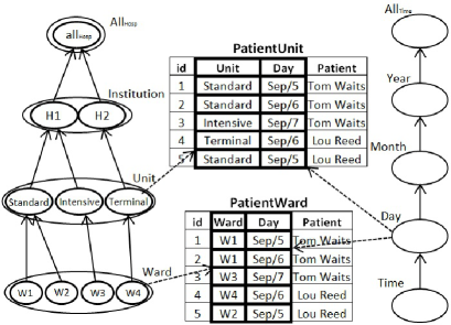
Figure 1: An extended multidimensional model

Elaborating on this example, it could be the case that there is a constraint imposed on dimensions and relations linked to their categories. For instance, one capturing that the intensive care unit was closed since August/2005: “No patient was in intensive care unit during the time after August /2005”. Again, through upward-navigation to the next category, we should conclude that the third tuple in table PatientWard should be discarded. This inter-dimensional constraint involves dimensions Hospital and Time (right-hand-side of Fig. 1), to which the ward and the day values in PatientWard are linked. $\Box$

The example shows a processing of data that involves changing the level of data linked to a dimension. This form of dimensional navigation may be required for query answering both in the downward and upward directions (Example 1 shows the latter). Our ontological multidimensional contexts support both.

Example 2 (ex. 1 cont.)

Two additional categorical relations, WorkingSchedules and Shifts (Table IV and Table IV), store shifts of nurses in wards and schedules of nurses in units. A query to Shifts asks for dates when Mark was working in ward W2, which has no answer with the extensional data in Table IV. Now, an institutional guideline states that if a nurse works in a unit on a specific day, he/she has shifts in every ward of that unit on the same day. Consequently, the last tuple in Table IV implies that Mark has shifts in both W1 and W2 on Sep/9. This date would be an answer obtained via downward navigation from the Standard unit to its wards (including W2). $\Box$

TABLE III: WorkingSchedules

	Unit	Day	Nurse	Type
1	Intensive	Sep/5	Cathy	cert.
2	Standard	Sep/5	Helen	cert.
3	Standard	Sep/6	Helen	cert.
4	Terminal	Sep/5	Susan	non-c.
5	Standard	Sep/9	Mark	non-c.

TABLE IV: Shifts

	Ward	Day	Nurse	Shift
1	W4	Sep/5	Cathy	night
2	W1	Sep/6	Helen	morning
3	W4	Sep/5	Susan	evening

Example 2 shows that downward navigation is necessary for query answering, in this case, for propagating data in WorkingSchedules at the Unit level down to Shifts at the lower Ward level). In this process a unit may drill-down to more than one ward, e.g. Standard unit is connected to wards W1 and W2), generating more than one tuple in Shifts.

Contexts should be represented as formal theories into which other objects, such as database instances, are mapped into, for contextual analysis, assessment, interpretation, additional processing, etc. [2]. Consequently, we show how to represent multidimensional contexts as logic-based ontologies (c.f. Section III). These ontologies represent and extend the HM multidimensional model (cf. Section II). Our ontological language of choice is Datalog$\pm$ [8]. It allows us to give a clear semantics to our ontologies, to support some forms of logical reasoning, and to apply some query answering algorithms. Furthermore, Datalog$\pm$ allows us to generate explicit data by completion where they are missing, which is particularly useful for data generation though dimensional navigation.

Our ultimate goal is to use multidimensional ontological contexts for data quality assessment [2], which is achieved by introducing and defining in the context relational predicates standing for the quality versions of relations in the original instance. Their definitions use additional conditions on data, to make them contain quality data. In this work, going beyond [2], the context also contains an ontology in Datalog$\pm$ that represents all the multidimensional elements shown in the examples above.

Our ontologies fall in the weakly-sticky (WS) class [8] of the Datalog$\pm$ family of languages [5] (cf. Section III) with separable equality generating dependencies (when used as dimensional constraints), which guarantees that conjunctive query answering can be done in polynomial time in data. We have developed and implemented a deterministic algorithm for boolean conjunctive query answering, which is based on a non-deterministic algorithm for WS Datalog$\pm$ [8]. The algorithm can be used with ontologies containing dimensional rules that support both upward or downward navigation (cf. Section IV). Section V shows how to use the ontology to populate the quality versions of original relations.

This paper is an extended abstract. We show concepts, ideas, ontologies, and mechanisms only by means of an extended example. The general approach and its analysis in detail will be presented in an extended version of this work.

II Preliminaries

We start from the HM multidimensional (MD) data model [12]. In it, dimensions represent the hierarchical data; and facts describe data as points in an MD space. A dimension is composed of a schema and an instance. A dimension schema includes a directed acyclic graph (DAG) of categories, which defines levels of the category hierarchy. A dimension hierarchy corresponds to a partial-order relation between the categories, a so-called parent-child relation. A dimension instance consists of set of members for each category. The instance hierarchy corresponds to a partial-order relation between members of categories, that parallels the parent-child relation between categories. Hospital and Time, at the right- and left-hand sides of Fig. 1, resp., are dimensions.

We extend the HM model with, among other elements, categorical relations, which can be seen as a generalization of fact tables, but at different dimension levels and not necessarily containing numerical data. Categorical relations represent the entities associated to the factual data. A categorical relation has a schema and an instance. A categorical relation schema is composed of a relation name and a list of attributes. Each attribute is either categorical or non-categorical. A categorical attribute takes as values the members of a category in a dimension. A non-categorical attribute takes values from an arbitrary domain.

Example 3 (ex. 1 cont.)

In Fig. 1, the categorical relation ${\it PatientWard(Ward,Day,Patient)}$ has its categorical attributes, Ward and Day, connected to the Hospital and Time dimensions. Patient is a non-categorical attribute with patient names as values (there could be a foreign key to another categorical relation that stores data of patients). $\Box$

Datalog$\pm$ [5] is a family of languages that extends plain Datalog with additional elements: (a) existential quantifiers in heads of tuple-generating dependencies (TGDs); (b) equality-generating dependencies (EGDs), that use equality in heads; and (c) negative constraints, that use $\bot$ in heads. With these extensions, Datalog$\pm$ captures ontological knowledge that cannot be expressed in classical Datalog.

Although the chase with these rules does not necessarily terminate, syntactic restrictions imposed on the set of rules aim to ensure decidability of conjunctive query answering, and is some cases, also tractability in data complexity. Datalog$\pm$ has sub-languages, such as linear, guarded, weakly-guarded, sticky, and weakly-sticky, that depend on the kind of predicates and syntactic interaction of TGD rules that appear in the Datalog$\pm$ program.

In this paper, our MD ontologies turn out to be written in weakly-sticky (WS) Datalog$\pm$. This sublanguage extends sticky Datalog$\pm$ [6]. WS Datalog$\pm$ allows joins in the body of TGDs, but with a milder restriction on the repeated variables. Boolean conjunctive query answering is tractable for WS Datalog$\pm$ [6].

III The Extended MD Model in Datalog$\pm$

We will represent our extended MD model as a Datalog$\pm$ ontology $\mathcal{M}$ that contains a schema $\mathcal{S}_{\mathcal{M}}$, an instance $\mathcal{D}_{\mathcal{M}}$, and a set of dimensional rules and constraints $\Sigma_{\mathcal{M}}$.  $\mathcal{S}_{\mathcal{M}}=\mathcal{K}\cup\mathcal{O}\cup\mathcal{R}$ is a finite set of predicates (relation names), where $\mathcal{K}$ is a set of category predicates (unary predicates), $\mathcal{O}$ is a set of parent-child predicates, i.e. partial-order relations between elements of adjacent categories, and $\mathcal{R}$ is a set of categorical predicates. In Example 1, ${\it K}$ contains, e.g. ${\it Ward}(\cdot),{\it Unit}(\cdot)$; $\mathcal{O}$ contains, e.g. a predicate for connections from Ward to Unit; and $\mathcal{R}$ contains, e.g. PatientWard. An instance, $\mathcal{D}_{\mathcal{M}}$, is a relational instance that gives (possibly infinite) extensions to the predicates in $\mathcal{S}_{\mathcal{M}}$, and satisfies a given set of TGDs, EGDs, and negative constraints $\Sigma_{\mathcal{M}}$ (cf. below). The constants for $\mathcal{D}_{\mathcal{M}}$ come from an infinite underlying domain.

The dimensional rules and constraints in $\Sigma_{\mathcal{M}}$ constitute the intentional part of $\mathcal{M}$. Rules (1)-((c)) below show the general form of elements of $\Sigma_{\mathcal{M}}$. In what follows, each $R_{i}(\bar{e}_{i};\bar{a}_{i})$ is a categorical atom, with $\bar{e}_{i}$ a sequence of categorical attributes (values) and $\bar{a}_{i}$ a sequence of non-categorical attributes; $D_{i}(e_{i},e^{\prime}_{i})$ is a parent-child atom with $e_{i},e^{\prime}_{i}$ parent/child elements, resp.; and $K_{i}(e_{i})$ is a category atom, with $e_{i}$ a category element. That is, $K_{i}\in\mathcal{K},D_{i}\in\mathcal{O}$, $R_{i}\in\mathcal{R}$. As an instance in (5) and (6), ${\it Unit}(u)$ is a category atom and ${\it UnitWard}(u,w)$ is a parent-child atom.

• To capture the referential constraint between a categorical attribute of a categorical relation and a category, we use a negative constraint, with $e\in\bar{e}_{i}$:

  $$\bot\ \leftarrow~{}R_{i}(\boldsymbol{\bar{e}_{i}};\bar{a}_{i}),\lnot K(e).$$ (1)

• A dimensional constraint is either an EGD of the form (2) (where $x,x^{\prime}$ also appear in the body) or a negative constraint of the form (3):

  $$x=x^{\prime}~{}\leftarrow~{} R_{i}(\boldsymbol{\bar{e}_{i}};\bar{a}_{i}),...,R_{j}(\boldsymbol{\bar{e}_{j}};\bar{a}_{j}),$$ (2)

  $$D_{n}(e_{n},e^{\prime}_{n}),...,D_{m}(e_{m},e^{\prime}_{m}).\vspace{-3mm}$$

  $$\bot~{}\leftarrow~{} R_{i}(\boldsymbol{\bar{e}_{i}};\bar{a}_{i}),...,R_{j}(\boldsymbol{\bar{e}_{j}};\bar{a}_{j}),$$ (3)

  $$D_{n}(e_{n},e^{\prime}_{n}),...,D_{m}(e_{m},e^{\prime}_{m}).\vspace{-4mm}$$

• A dimensional rule is a Datalog$\pm$ TGD of the form:

  $$\exists\bar{a}_{z}\;R_{k}(\bar{e}_{k};\bar{a}_{k})\ ~{}\leftarrow R_{i}(\boldsymbol{\bar{e}_{i}};\bar{a}_{i}),...,R_{j}(\boldsymbol{\bar{e}_{j}};\bar{a}_{j}),$$

  $$D_{n}(e_{n},e^{\prime}_{n}),...,D_{m}(e_{m},e^{\prime}_{m}).$$

  poto
  Here, $\bar{a}_{z}\subseteq\bar{a}_{k}$, $\bar{e}_{k}\subseteq\bar{e}_{i}\cup...\cup\bar{e}_{j}\cup\{e_{n},...,e_{m}\}\cup\{e^{\prime}_{n},...,e^{\prime}_{m}\}$ and $\bar{a}_{k}\!\smallsetminus\!\bar{a}_{z}\subseteq\bar{a}_{i}\cup...\cup\bar{a}_{j}$. Furthermore, shared variables in bodies of TGDs correspond only to categorical attributes of categorical relations.

With rule ((c)) (an example is (7) below), the possibility of doing dimensional navigation is captured by joins between categorical predicates, e.g. $R_{i}(\boldsymbol{\bar{e}}_{i};\bar{a}_{i}),...,R_{j}(\boldsymbol{\bar{e}}_{j};\bar{a}_{j})$ in the body, and parent-child predicates, e.g. $D_{n}(e_{n},e^{\prime}_{n}),...,D_{m}(e_{m},e^{\prime}_{m})$. Rule ((c)) allows navigation in both upward and downward directions. The direction of navigation is determined by the level of categorical attributes that participate in the join in the body. Assuming the join is between $R_{i}(\bar{e}_{i};\bar{a}_{i})$ and $D_{n}(e_{n},e^{\prime}_{n})$, upward navigation is enabled when $e^{\prime}_{n}\in\bar{e}_{i}$ (i.e. $e^{\prime}_{n}$ appears in $R_{i}(\bar{e}_{i};\bar{a}_{i})$) and $e_{n}\in\bar{e}_{k}$ (i.e $e_{n}$ appears in the head). On the other hand, if $e_{n}$ occurs in $R_{i}$ and $e^{\prime}_{n}$ occurs in $R_{k}$, then downward navigation is enabled, from $e_{n}$ to $e^{\prime}_{n}$.

The existential variables in ((c)) make up for missing non-categorical attributes due to different schemas (i.e. the existential variables may appear in positions of non-categorical attributes but not in categorical attributes). As a result, when drilling down, for each tuple of a categorical relation linked to a parent member, the rule generates tuples for all the child members of the parent member (or children specifically indicated in the body).

Example 4 (ex. 3 cont.)

The categorical attribute Unit in categorical relation PatientUnit takes values from the Unit category. We use a constraint of the form (1). Similar constraints are in the ontology that capture the connection between other categorical relations and their corresponding categories.

$$\bot ~{}\leftarrow~{}{\it PatientUnit(\boldsymbol{u},\boldsymbol{d};p)},\lnot{\it Unit}(u).$$ (5)

poto
For the constraint in Example 1 requiring “No patient was in intensive care unit during the time after August 2005”, we use a dimensional constraint of the form (3):

$$\bot~{}\leftarrow~{} {\it PatientWard(\boldsymbol{w},\boldsymbol{d};p)},{\it UnitWard}({\tt Intensive},w),$$

$${\it MonthDay}({\tt August/2005},d).$$

poto
Similarly, the following rule, of form (2), states that “All the thermometers used in a unit are of the same type”:

$$t=t^{\prime}~{}\leftarrow~{} {\it Thermometer(\boldsymbol{w},\boldsymbol{t};n)},{\it Thermometer(\boldsymbol{w^{\prime}},\boldsymbol{t^{\prime}};n^{\prime})},$$

$${\it UnitWard(u,w)},{\it UnitWard(u,w^{\prime})},$$ (6)

poto
with ${\it Thermometer(Ward,Thermometertype;}$${\it Nurse})$ a categorical relation with thermometers used by nurses in wards.

Finally, the following dimensional rules of the form ((c)) capture how data in PatientWard and WorkingSchedules generate data for PatientUnit and Shifts, resp.:

$${\it PatientUnit(\boldsymbol{u},\boldsymbol{d};p)}~{}\leftarrow~{} {\it PatientWard(\boldsymbol{w},\boldsymbol{d};p)},$$ (7)

$${\it UnitWard(u,w)}.$$

$$\exists z\;{\it Shifts(\boldsymbol{w},\boldsymbol{d};n,z)}~{}\leftarrow~{} {\it WorkingSchedules(\boldsymbol{u},\boldsymbol{d};n,t)},$$

$${\it UnitWard(u,w)}.$$ (8)

poto

In (7), dimension navigation is enabled by the join between PatientWard and UnitWard. The rule generates data for PatientUnit (at a the higher level of Unit) from PatientWard (at the lower level of Ward) via upward navigation. Notice that (7) is in the general form ((c)), but since in this case the schemas of the two involved categorical relations match, no existential quantifiers are necessary.

Rule (8) captures downward navigation while it generates data for Shifts (at the level of Ward) from WorkingSchedules (at the level of Unit). In this case, the schemas of the two categorical relations do not match. So, the existential variable $z$ represents missing data for the shift attribute. $\Box$

It is possible to verify that the Datalog$\pm$ MD ontologies with rules of the forms (1)-((c)) are weakly-sticky. This follows from the fact that shared variables in the body of dimensional rules, as defined in ((c)), may occur only in positions of categorical attributes, where only limited values may appear, which depends on the assumption that the MD ontology has a fixed dimensional structure, in particular, with a fixed number of category members. No new category member is generated when applying the dimensional rules of the form ((c)).

The separability property [7, 8] in relation to the interaction of dimensional EGDs of the form (2) and TGDs of the form ((c)) must be checked independently. However, when the EGDs have only categorical variables in the heads, the separability condition holds, which is the case with rule (6).

Example 5 (ex. 2 and 4 cont.)

To illustrate query answering via downward navigation, reconsider the query about the dates that Mark works in W1: $\mathcal{Q}^{\prime}(d)\leftarrow{\it Shifts}({\tt W1},d,{\tt Mark},s)$. Considering (8) and the last tuple in WorkingSchedules, the chase will generate a new tuple in Shifts for Mark on Sep/9 in W2, with a fresh null value for his shift, reflecting incomplete knowledge about this attribute at the lower level. So, the answer to the query via (8) is Sep/9. $\Box$

The general TGD ((c)) only captures downward navigation when there is incomplete data about the values of non-categorical attributes, because existential variables are only non-categorical. However, in some cases we may have incomplete data about the categorical attributes, i.e. about parents and children involved in downward navigation.

TABLE V: DischargePatients

	Inst.	Day	Patient
1	H1	Sep/9	Tom Waits
2	H1	Sep/6	Lou Reed
3	H2	Oct/5	Elvis Costello

Example 6 (ex. 1 cont.)

There is an additional categorical relation DischargePatients (Table V) with data about patients leaving an institution. Since each of them was in exactly one of the units, DischargePatient should generate data for PatientUnit through downward navigation from the Institution level to the Unit level. Since we do not have knowledge about which unit at the lower level has to be specified, the following rule could be used:

$$\exists u\;{\it InstitutionUnit(i,u)}, {\it PatientUnit(\boldsymbol{u},\boldsymbol{d};p)}~{}\leftarrow~{}$$ (9)

$${\it DischargePatients(\boldsymbol{i},\boldsymbol{d};p)},$$

poto
which is not of the form ((c)), because it has an existentially quantified categorical variable, $u$, for units. It allows downward navigation while capturing incomplete data about units, and represents disjunctive knowledge at level of units. $\Box$

The general form of (9), for this type of downward navigation is as follows:

$$\exists\bar{z}\;R_{k}(\bar{e}_{k};\bar{a}_{k}),D_{n}(e_{n},e^{\prime}_{n}) ,...,D_{m}(e_{m},e^{\prime}_{m})\ \ \leftarrow$$ (10)

$$R_{i}(\boldsymbol{\bar{e}_{i}};\bar{a}_{i}),...,R_{j}(\boldsymbol{\bar{e}_{j}};\bar{a}_{j}),$$

poto
where $\bar{z}\subseteq\bar{e}_{k}\cup\bar{a}_{k}\cup\{e_{n},...,e_{m}\}\cup\{e^{\prime}_{n},...,e^{\prime}_{m}\}$ and $\bar{e}_{k}\cup\{e_{n},...,e_{m}\}\cup\{e^{\prime}_{n},...,e^{\prime}_{m}\}\!\smallsetminus\!\bar{z}\subseteq\bar{e}_{i}\cup...\cup\bar{e}_{j}$ and $\bar{a}_{k}\!\smallsetminus\!\bar{z}\subseteq\bar{a}_{i}\cup...\cup\bar{a}_{j}$, and the categorical attributes of $R_{i},\ldots,R_{j}$ refer to categories that are at a higher or same level than the categorical attributes of $R_{k}$. (In (9), categories ${\it Institution}$ and ${\it Day}$ for ${\it DischargePatients}$ are higher and same level, resp. than ${\it Unit}$ and ${\it Day}$ for ${\it PatientUnit}$.)

If the MD ontology also includes rules of the form (10), it still is weakly-sticky. This is because, despite the fact that these rules may generate new members (nulls), they can only generate a limited number of such members (because the rule only navigates in downward direction), i.e. there is no cyclic behavior. With these new rules, EGDs with only categorical attributes in heads do not guarantee separability anymore. So, checking this condition becomes application dependent.

IV Query Answering on MD Ontologies

Weakly-stickyness guarantees that boolean conjunctive query answering from our MD contextual ontologies becomes tractable in data complexity [8]. Then, answering open conjunctive queries from the MD ontology is also tractable [10].

We have developed and implemented a deterministic algorithm, DeterministicWSQAns, for answering boolean conjunctive queries from Datalog$\pm$ MD contextual ontologies. The algorithm is based on a non-deterministic algorithm, WeaklyStickyQAns, for WS Datalog$\pm$ that runs in polynomial time in the size of extensional database [8].

Given a set of WS TGDs, a boolean conjunctive query, and an extensional database, WeaklyStickyQAns builds an “accepting resolution proof schema”, a tree-like structure which shows how query atoms can be entailed from the extensional instance. The algorithm rejects if there is no resolution proof schema; otherwise it builds it and accepts.

Our deterministic algorithm, DeterministicWSQAns, applies a top-down backtracking search for accepting resolution proof schemas. Starting from the query, the algorithm resolves the atoms of the query, from left to right. In each step, an atom is resolved either by finding a substitution that maps the atom to a ground atom in the extensional database (which makes a leaf node) or by applying a TGD rule that entails the atom (building a subtree). The decision at each step is stored on a stack to be restored later if the algorithm fails to entail the atoms of the query in the next steps. The algorithm accepts if it resolves all the atoms in the query (the content of the stack specifies the decisions that lead to the accepting resolution proof schema), and rejects if it cannot resolve an atom, no matter what decisions have been made before.

In this deterministic approach, possible substitutions of constants for query variables are derived by the ground atoms in the extensional database (as opposed to the non-deterministic version of the algorithm that guesses applicable substitutions). This enables us to extend DeterministicWSQAns for finding answers to open conjunctive queries, by building resolution proof schemas for all possible substitutions.

WeaklyStickyQAns runs in polynomial time in the size of the extensional database [6]. It can be proved that DeterministicWSQAns also runs in polynomial time. None of these algorithms are first-order (FO) query rewriting algorithms, which do exist for the Datalog$\pm$ more restrictive syntactic classes, e.g. linear and sticky [5, 6].

The MD ontologies to which the complexity results and algorithms above apply support both upward and downward navigation. However, for simpler MD ontologies that support only upward navigation (which can be syntactically detected from the form of the dimensional rules), we developed a methodology for conjunctive query answering based on FO query rewriting. The rewritten query can be posed directly to the extensional database. Ontologies of this kind are common and natural in real world applications (Example 1 shows such a case). Interestingly, these “upward-navigating” MD ontologies do not necessarily fall into any of the “good” cases of Datalog$\pm$ mentioned above.

The algorithms mentioned in this section are rather proofs of concept than algorithms meant to be used with massive data. It is ongoing work the development and implementation of scalable polynomial time algorithms for answering open conjunctive queries.

V MD Ontologies and Data Quality

In this section, we show how a Datalog$\pm$ MD ontology can be a part of -and used in- a context for data quality assessment or cleaning. Fig. 2 shows such a context and the way it is used. The central idea in [2] is that the original instance $\mathcal{D}$ (on the left-hand-side) is to be assessed or cleaned through the context in the middle. This is done by mapping $\mathcal{D}$ into the contextual schema/instance $\mathcal{C}$. The context may have additional data, predicates ($C_{i}$), data quality predicates ($P_{i}$) specifying single quality requirements, and access to external data sources ($E_{i}$) for data assessment or cleaning. The clean version of $\mathcal{D}$ is on the right-hand-side, with schema $\mathcal{S}^{q}$, which is a copy of $\mathcal{D}$’s schema [2].

The new element in the context is the MD ontology $\mathcal{M}$, which interacts with $\mathcal{C}$, and represents the dimensional elements of the context. The categorical relations in $\mathcal{M}$ provide dimensional data for the relations in $\mathcal{C}$ and for quality predicates in $\mathcal{P}$. $\mathcal{C}$ also gets extensional data from initial database, $\mathcal{D}$, and external sources. Here we concentrate on data cleaning, which here amounts to obtaining clean answers to queries, in particular, about clean extensions ($S^{q}_{i}$) for the original database relations ($S_{i}$) (a particular case of clean query answering [2]).

The quality versions $S^{q}_{i}$ are specified in terms of the relations in $\mathcal{C}$ and quality predicates, $P_{i}$. The data for the latter may be already in the context or come from $\mathcal{D}$, the ontology $\mathcal{M}$, or external sources. The problems become: (a) computing quality versions $S_{i}^{q}$ of the original predicates, and (b) computing quality answers to queries $\mathcal{Q}$ expressed in terms of those original predicates. The second problem is solved by rewriting the query as $\mathcal{Q}^{q}$, which is expressed (and answered) in terms of predicates $S^{q}_{i}$. Answering it is the part of the query answering process that may invoke dimensional navigation and data generation as illustrated in previous sections. Problem (a) is a particular case of (b).

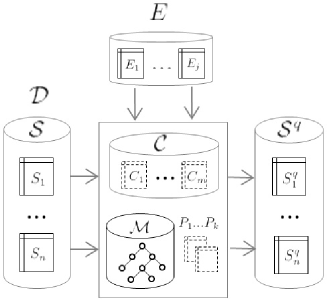
Figure 2: An MD context for data quality assessment

Example 7

(ex. 4 cont.) A query $\mathcal{Q}$ about Tom Waits’ temperatures is initially expressed in terms of the initial predicates Measurements, but is rewritten into a query expressed and an-

swered via its quality extension ${\it Measurements}^{q}$ (see [2] for more details). More specifically, the query is about  “The body temperatures of Tom Waits on September 5 taken around noon by a certified nurse with a thermometer of brand B1”:

$$\mathcal{Q}(t,p,v)\ \leftarrow \ {\it Measurements(t,p,v)},p={\tt Tom\;\;Waits},$$

$$~{}~{}{\tt Sep/5\mbox{-}11\mbox{:}45}\leq t\leq{\tt Sep/5\mbox{-}12\mbox{:}15}.$$

poto

Measurements, as initially given, does not contain information about nurses or thermometers. Hence the expected conditions are not expressed in the query. According to the general contextual approach in [2], predicate Measurement has to be logically connected to the context, conceiving it as a footprint of a “broader” contextual relation that is given or built in the context, in this case one with information about thermometer brands ($b$) and nurses’ certification status ($y$):

$${\it Measurement}^{\prime}(t,p,v,y,b) \leftarrow {\it Measurement}^{c}(t,p,v),$$

$${\it TakenByNurse}(t,p,n,y),{\it TakenWithTherm}(t,p,b),$$

poto

where ${\it Measurement}^{c}$ is a contextual copy of Measurement, i.e. the latter is mapped into the context. If we want quality measurements data, we impose the quality conditions:

$${\it Measurement}^{q}(t,p,v) \leftarrow {\it Measurement}^{\prime}(t,p,v,y,b),$$

$$y={\tt Certified},\ b={\tt B1},$$

poto

with the auxiliary predicates defined by:

$${\it TakenByNurse}(t,p,n,y) \leftarrow {\it WorkingSchedules}(u,d;n,y),$$

$${\it DayTime}(d,t),{\it PatientUnit}(u,d;p).$$

$${\it TakenWithTherm}(t,p,b) \leftarrow {\it PatientUnit}(u,d;p),$$

$${\it DayTime}(d,t),b={\tt B1},u={\tt Standard}.$$

poto

Here, DayTime is parent/child relation in Time dimension), and the last definition right above is capturing as a rule the guideline from Example 1, at the level of relation PatientUnit.

Summarizing, TakenByNurse and TakenWithTherm are contextual predicates (shown in Fig. 2 as $P_{i}$). PatientWard and WorkingSchedules are categorical relations.

To obtain quality answers to the original query, we pose to the ontology the new query:

$$\mathcal{Q}^{q}(t,p,v)\ \leftarrow \ {\it Measurements(t,p,v)^{q}},\ p={\tt Tom\;\;Waits},$$

$${\tt Sep/5\mbox{-}11\mbox{:}45}\leq t\leq{\tt Sep/5\mbox{-}12\mbox{:}15}.$$

poto

Answering it, which requires evaluating TakenWithTherm, triggers upward dimensional navigation from Ward to Unit, when requesting data for categorical relation PatientUnit. More specifically, dimensional rule (7) is used for data generation, and each tuple in PatientWard generates one tuple in PatientUnit, with its unit obtained by rolling-up . $\Box$

VI Conclusions

We have described in general terms how to specify in Datalog$\pm$ a multidimensional ontology that extends a multidimensional data model. We have identified some properties of these ontologies in terms of membership to known classes of Datalog$\pm$, the complexity of conjunctive query answering, and the existence of algorithms for the latter task. Finally, we showed how to apply the ontologies to multidimensional and contextual data quality, in particular, for obtaining quality answers to queries through dimensional navigation. MD contexts are also of interest outside applications to data quality. They can be seen as logical extensions of the MD data model.

Acknowledgments: Research funded by NSERC Discovery, and the NSERC Strategic Network on Business Intelligence (BIN). L. Bertossi is a Faculty Fellow of IBM CAS. We thank Andrea Cali and Andreas Pieris for useful information and conversations on Datalog$\pm$.

References

- [1] C. Batini, and M. Scannapieco. Data Quality: Concepts, Methodologies and Techniques. Springer, 2006.
- [2] L. Bertossi, F. Rizzolo, and J. Lei. Data Quality is Context Dependent. Proc. WS on Enabling Real-Time Business Intelligence, Collocated with VLDB, 2010, pp. 52-67.
- [3] L. Bertossi. Database Repairing and Consistent Query Answering. Morgan & Claypool, 2011.
- [4] C. Bolchini, E. Quintarelli, and L. Tanca. CARVE: Context-aware automatic view definition over relational databases. Information Systems, 2013, 38:45-67.
- [5] A. Cali, G. Gottlob, and T. Lukasiewicz. Datalog: a unified approach to ontologies and integrity constraints. Proc. ICDT, 2009, pp. 14-30.
- [6] A. Cali, G. Gottlob, and A. Pieris. Query answering under non-guarded rules in datalog+/-. Proc. RR, 2010, pp. 1-17.
- [7] A. Cali, G. Gottlob, and A. Pieris. Querying conceptual schemata with expressive equality constraints. Proc. ER, 2011, pp. 161-174.
- [8] A. Cali, G. Gottlob, and A. Pieris. Towards more expressive ontology languages: The query answering problem. Artificial Intelligence, 2012, 193:87-128.
- [9] D. Calvanese, G. Giacomo, D. Lembo, M. Lenzerini, and R. Rosati. Towards more expressive ontology languages: The query answering problem. J. of Automated Reasoning, 2007, 39:385-429.
- [10] R. Fagin, P. G. Kolaitis, R. J. Miller, and L. Popa. Data exchange: semantics and query answering. Theoretical Computer Science, 2005, 336:89-124.
- [11] G. Gottlob, G. Orsi, and A. Pieris. Ontological queries: rewriting and optimization. Proc. ICDE, 2011, pp. 2-13.
- [12] C. Hurtado, C. Gutierrez, and A. Mendelzon. Capturing summarizability with integrity constraints in OLAP. ACM Transactions on Database Systems, 2005, 30:854-886.
- [13] L. Jiang, A. Borgida, and J. Mylopoulos. Towards a compositional semantic account of data quality attributes. Proc. ER, 2008, pp. 55-68.
- [14] A. Maleki, L. Bertossi, and F. Rizzolo. Multidimensional contexts for data quality assessment. Proc. AMW, 2012, pp. 196-209.
- [15] D. Martinenghi, and R. Torlone. Querying databases with taxonomies. Proc. ER, 2010, pp. 377-390.