Topology and field strength
in spherical, anelastic dynamo simulations

Abstract

Context. Numerical modelling of convection driven dynamos in the Boussinesq approximation revealed fundamental characteristics of the dynamo-generated magnetic fields and the fluid flow. Because these results were obtained for an incompressible fluid of constant density, their validity for gas planets and stars remains to be assessed. A common approach is to take some density stratification into account with the so-called anelastic approximation.

Aims. The validity of previous results obtained in the Boussinesq approximation is tested for anelastic models. We point out and explain specific differences between both types of models, in particular with respect to the field geometry and the field strength, but we also compare scaling laws for the velocity amplitude, the magnetic dissipation time, and the convective heat flux.

Methods. Our investigation is based on a systematic parameter study of spherical dynamo models in the anelastic approximation. We make use of a recently developed numerical solver and provide results for the test cases of the anelastic dynamo benchmark.

Results. The dichotomy of dipolar and multipolar dynamos identified in Boussinesq simulations is also present in our sample of anelastic models. Dipolar models require that the typical length scale of convection is an order of magnitude larger than the Rossby radius. However, the distinction between both classes of models is somewhat less explicit than in previous studies. This is mainly due to two reasons: we found a number of models with a considerable equatorial dipole contribution and an intermediate overall dipole field strength. Furthermore, a large density stratification may hamper the generation of dipole dominated magnetic fields. Previously proposed scaling laws, such as those for the field strength, are similarly applicable to anelastic models. It is not clear, however, if this consistency necessarily implies similar dynamo processes in both settings.

1 Introduction

Magnetic fields of low-mass stars and planets are maintained by currents resulting from the motion of a conducting fluid (or gas) in their interiors. Because the magnetic field acts back on the flow via the Lorentz force, the hydrodynamic dynamo problem is intrinsically nonlinear. Moreover, a sufficiently complex flow and magnetic field geometry has to be assumed in order to enable dynamo action. Further complications result from tiny diffusivities, such as small kinematic viscosities, which introduce small dynamic length scales compared to stellar or planetary radii. Thus, self-consistent simulations of natural dynamos are not only three-dimensional, but a vast range of spatial and temporal scales has to be resolved. These difficulties prevented a direct numerical treatment of the dynamo problem for a significant time. Only for the last 20 years increasing computer power made global, direct numerical simulations feasible, in particular for the geodynamo problem (e.g. Glatzmaier & Roberts 1995; Kageyama & Sato 1997; Kuang & Bloxham 1997; Christensen et al. 1998; Sarson et al. 1998; Katayama et al. 1999; Buffett 2000; Dormy et al. 2000); for an early cylindrical annulus model of the geodynamo see Busse (1975). In these simulations, an incompressible conducting fluid was considered, and the Boussinesq approximation was applied. Intensive and systematic parameter studies revealed fundamental properties of these models related to their field and flow topologies, their field strength, their velocity amplitudes, their advective heat transport, or their time dependence (e.g. Christensen et al. 1999; Grote et al. 2000; Kutzner & Christensen 2002; Busse & Simitev 2006; Christensen & Aubert 2006; Sreenivasan & Jones 2006; Busse & Simitev 2010; Hori et al. 2010; Landeau & Aubert 2011; Schrinner et al. 2012; Yadav et al. 2013a). The simplifying assumption of constant density in Boussinesq models, however, is probably not justified for gas planets or stars, in which the density typically varies over many scale heights. An alternative approach, which takes compressibility into account, is the so-called anelastic approximation (Ogura & Phillips 1962; Gough 1969; Gilman & Glatzmaier 1981). In anelastic models, the density varies with radius, but its time derivative is neglected in the continuity equation and the mass flux is solenoidal (e.g. Glatzmaier 1984; Braginsky & Roberts 1995; Lantz & Fan 1999; Miesch et al. 2000; Brun et al. 2004; Browning et al. 2004). Consequently, fast travelling sound waves are filtered out and, compared to fully compressible models, larger time steps in the discretisation scheme may be reached. In this article, we carry out a systematic parameter study of global dynamo simulations in the anelastic approximation guided by well known results of Boussinesq models. In this way, we intend to point out specific differences between anelastic and Boussinesq models and assess the validity of previous findings obtained in the Boussinesq approximation. A similar approach was followed by Gastine et al. (2012) and Yadav et al. (2013b). We compare our results with their findings and discuss some differences we obtained for our varied sample of models. The conditions for the generation of large-scale, dipolar fields (Section 3) and the test of the flux-based scaling law for the magnetic field strength (Section 4), originally proposed by Christensen & Aubert (2006) for Boussinesq models, are revisited. We argue that the typical length scale of convection relative to the Rossby radius is of crucial importance for the resulting field topology (see also Schrinner et al. 2012) and show that larger magnetic Prandtl numbers are required to obtain dipolar solutions with increasing density contrast. Furthermore, the flux-based scaling laws derived for Boussinesq models seem to hold in the anelastic approximation as well. However, because of their general validity, the flux-based scaling laws might not be appropriate to distinguish between different conditions for magnetic field generation.

The paper is organised as follows: Section 2 introduces the anelastic models considered here and the recently developed numerical solver; results for a numerical benchmark are given in Appendix A. In Section 3, we present new evidence for the existence of a class of dynamos dominated by an axial dipole and a class of models with a more variable magnetic field geometry. Various scaling laws originally derived for Boussinesq models are tested and discussed in Section 4, and we give some conclusions in Section 5.

2 Dynamo calculations

2.1 The anelastic approximation

Convection of a gas or a compressible fluid in the interior of planets and stars takes place on a vast range of spatial and temporal scales. Sound waves excited in convection zones, for example, have very short oscillation periods compared to the turnover time of convection or the magnetic diffusion time relevant for the generation of magnetic fields. Thus, extremely small timesteps would be required to resolve these waves in numerical dynamo models. To avoid this problem, simplifications of the governing equations are often applied. The anelastic approximation used in this study advantageously filters out sound waves (Ogura & Phillips 1962; Gough 1969; Gilman & Glatzmaier 1981); it is motivated by the idea that the superadiabatic temperature gradient driving convection in planetary or stellar convection zones is tiny. The thermodynamic variables are then decomposed into the sum of (close to adiabatic) reference values, denoted here by an overbar, and perturbations, denoted by a prime,

$$\varrho=\overline{\varrho}+\varrho^{\prime},\quad T=\overline{T}+T^{\prime},\quad P=\overline{P}+P^{\prime}\,.$$ (1)

Subsequently, the anelastic equations result from the ‘thermodynamic linearization’ around the reference state. It should be stressed that a number of different formulations of the anelastic problem can be found in the literature (e.g. Glatzmaier 1984; Braginsky & Roberts 1995; Lantz & Fan 1999; Miesch et al. 2000; Brun et al. 2004; Rogers & Glatzmaier 2005; Jones & Kuzanyan 2009; Alboussière & Ricard 2013). We follow here the approach introduced by Lantz & Fan (1999) and Braginsky & Roberts (1995), also known as LBR-approximation. They noticed that the only relevant thermodynamic variable in the equation of motion is the entropy, if the reference state is assumed to be close to adiabatic. Further advantages of the LBR-equations over others are that they give a mathematically consistent, asymptotic limit of the full, general equations (Jones et al. 2011) and guarantee the conservation of energy (Brown et al. 2012). Moreover, the LBR-equations were used to formulate anelastic dynamo benchmarks (Jones et al. 2011). The presentation of the equations given here follows the benchmark paper and Jones et al. (2009).

2.2 Basic assumptions

We consider a perfect, electrically conducting gas in a rotating spherical shell with an inner boundary at $r=r_{i}$ and an outer boundary at $r=r_{o}$. The aspect ratio of the shell is then defined by $\chi=r_{i}/r_{o}$. Convection in our simulations is driven by an imposed entropy difference, $\Delta s$, between the inner and the outer boundary. As discussed above, $\Delta s$ is assumed to be small. This implies small convective velocities compared to the speed of sound. For consistency, we also require that the Alfvén velocity of the magnetic field is small. Moreover, the kinematic viscosity $\nu$, the thermal diffusivity $\kappa$ and the magnetic diffusivity $\eta$ are constants throughout in this paper. Following Jones et al. (2011) we represent the heat flux in our models in terms of the entropy gradient instead of the temperature gradient. This assumption relies on wide-spread ideas about turbulent mixing (Braginsky & Roberts 1995) but does not follow from first principles. Applying this simplification allows us to consider the entropy as the only relevant thermodynamic variable in the formulation of the anelastic problem.

2.3 The reference state

The reference state of our models is a solution of the hydrostatic equations for an adiabatic atmosphere. Moreover, the centrifugal acceleration is neglected and we assume that gravity varies radially, $\mathbf{g}=-GM\mathbf{\hat{r}}/r^{2}$ with G being the gravitational constant and $M$ the central mass of the star or the planet. This admits a polytropic solution for the reference atmosphere,

$$\overline{P}=P_{c}\,w^{n+1},\quad\overline{\varrho}=\varrho_{c}\,w^{n},\quad\overline{T}=T_{c}\,w,\quad w=c_{0}+\frac{c_{1}d}{r},$$ (2)

with the polytropic index $n$ and $d=r_{o}-r_{i}$. We note that $n$ defines the value of the adiabatic exponent $\gamma$, or the ratio of specific heats $c_{p}/c_{v}$, via $\gamma=(n+1)/n$. The values  $P_{c}$, $\varrho_{c}$, and $T_{c}$ are taken midway between the inner and the outer boundary and serve as units for the reference-state variables. Moreover, the constants $c_{0}$ and $c_{1}$ in (2) are defined as

$$c_{0}=\frac{2w_{0}-\chi-1}{1-\chi},\quad c_{1}=\frac{(1+\chi)(1-w_{o})}{(1-\chi)^{2}},$$ (3)

with

$$w_{0}=\frac{\chi+1}{\chi\exp(N_{\varrho}/n)+1},\quad w_{i}=\frac{1+\chi-w_{o}}{\chi},$$ (4)

and $N_{\varrho}=\ln{(\varrho_{i}/\varrho_{o})}$, where $\varrho_{i}$ and $\varrho_{o}$ denote the reference state density at the inner and outer boundary, respectively. We emphasise again that convection in our models is not driven by the reference state, or by the choice of a particular polytropic index $n$, but by an imposed entropy difference $\Delta s$ between the boundaries.

2.4 The non-dimensional equations

The use of non-dimensional equations minimizes the number of free parameters and is a prerequisite for a systematic parameter study. We choose the shell width $d$ as the fundamental length scale of our models, time is measured in units of $d^{2}/\eta$, and $\Delta s$ is the unit of entropy. The magnetic field is then measured in units of $\sqrt{\Omega\varrho_{c}\mu\eta}$ where $\Omega$ is the rotation rate and $\mu$ the magnetic permeability. Finally, our dynamo models are solutions for the velocity $\mathbf{v}$, the magnetic field $\mathbf{B}$, and the entropy $s$ of the following, non-dimensional equations,

$$\frac{\partial\mathbf{v}}{\partial t}+\mathbf{v}\cdot\nabla\mathbf{v} = Pm\,\big{[}-\frac{1}{E}\nabla\frac{P^{\prime}}{w^{n}}+\frac{Pm}{Pr}Ra\frac{s}{r^{2}}\mathbf{\hat{r}}-\frac{2}{E}\,\mathbf{\hat{z}}\times\mathbf{v}$$ (5)

$$+\mathbf{F}_{\nu}+\frac{1}{E\,w^{n}}(\nabla\times\mathbf{B})\times\mathbf{B}\big{]}\,,$$

$$\frac{\partial\mathbf{B}}{\partial t} = \nabla\times(\mathbf{v}\times\mathbf{B})+\nabla^{2}\mathbf{B}\,,$$ (6)

$$\frac{\partial s}{\partial t}+\mathbf{v}\cdot\nabla s = w^{-n-1}\frac{Pm}{Pr}\nabla\cdot\left(w^{n+1}\,\nabla s\right)$$ (7)

$$+\frac{Di}{w}\left[E^{-1}w^{-n}(\nabla\times\mathbf{B})^{2}+Q_{\nu}\right]\,,$$

$$\nabla\cdot\left(w^{n}\mathbf{v}\right) = 0\,,$$ (8)

$$\nabla\cdot\mathbf{B} = 0\,.$$ (9)

In (5) we used the viscous force $\mathbf{F}_{\nu}=w^{-n}\nabla\mathbf{S}$ with the rate of strain tensor

$$S_{ij}=2w^{n}\left(e_{ij}-\frac{1}{3}\delta_{ij}\nabla\cdot\mathbf{v}\right),\quad e_{ij}=\frac{1}{2}\left(\frac{\partial v_{i}}{\partial x_{j}}+\frac{\partial v_{j}}{\partial x_{i}}\right)\,.$$ (10)

Moreover, the dissipation parameter $Di$ and the viscous heating $Q_{\nu}$ in (7) are given by

$$Di=\frac{c_{1}Pr}{PmRa}\,,$$ (11)

and

$$Q_{\nu}=2\left[e_{ij}e_{ij}-\frac{1}{3}(\nabla\cdot\mathbf{v})^{2}\right]\,.$$ (12)

The system of equations (5)–(9) is governed by a number of dimensionless parameters. These are the Rayleigh number $Ra$, the Ekman number $E$, the Prandtl number $Pr$, and the magnetic Prandtl number $Pm$. Together with the aspect ratio $\chi$, the polytropic index $n$, and the number of density scale heights $N_{\varrho}$ defining the reference state, our models are therefore fully determined by seven dimensionless parameters:

$$Ra = \frac{GMd\Delta s}{\nu\kappa c_{p}},\quad Pr=\frac{\nu}{\kappa},\quad Pm=\frac{\nu}{\eta},\quad E=\frac{\nu}{\Omega d^{2}}\,,$$

$$N_{\varrho} = \ln\left(\frac{\varrho_{i}}{\varrho_{o}}\right),\quad n,\quad\chi=\frac{r_{i}}{r_{o}}\,.$$ (13)

Following Jones et al. (2009), we also considered a linearized form of equations (5) and (7) to calculate some critical Rayleigh numbers for the onset of convection. These are listed in Table LABEL:tab:rac.

2.5 Boundary conditions

The mechanical boundary conditions are impenetrable and stress free on both boundaries,

$$v_{r}=\frac{\partial}{\partial r}\left(\frac{v_{\theta}}{r}\right)=\frac{\partial}{\partial r}\left(\frac{v_{\phi}}{r}\right)=0\qquad\text{on}\quad r=r_{i}\quad\text{and}\quad r=r_{o}\,.$$ (14)

Furthermore, the magnetic field matches a potential field outside the fluid shell. The choice of these boundary conditions requires that the total angular momentum is conserved (Jones et al. 2011). Finally, the entropy is fixed on the inner and the outer boundary with

$$s=\Delta s\qquad\text{on}\quad r=r_{i},\quad\text{and}\quad s=0\qquad\text{on}\quad r=r_{o}\,.$$ (15)

2.6 Output parameters

We use a number of non-dimensional output parameters to characterize our numerical dynamo models. These are mostly based on the kinetic and magnetic energy densities,

$$E_{\mathrm{k}}=\frac{1}{2\,V}\int_{V}\,w^{n}\mathbf{v}^{2}\,\mathrm{d}V\,\,\,\mbox{and}\qquad E_{\mathrm{m}}=\frac{1}{2\,V}\frac{Pm}{E}\int_{V}\,\mathbf{B}^{2}\,\mathrm{d}V\,,$$ (16)

where the integrals are taken over the volume of the fluid shell $V$. A non-dimensional measure for the velocity amplitude is then the magnetic Reynolds number, $Rm=\sqrt{2E_{\mathrm{k}}}$, or the Rossby number, $Ro=\sqrt{2E_{\mathrm{k}}}E/Pm$. To distinguish models with different field geometries it turned out to be useful to introduce also a local Rossby number, $Ro_{\ell}=Ro_{c}\,\ell_{c}/\pi$. Here, $\ell_{c}$ stands for the mean harmonic degree of the velocity component $\mathbf{v}_{c}$ from which the mean zonal flow has been subtracted (Schrinner et al. 2012),

$$\ell_{c}=\sum_{\ell}\ell\frac{<w^{n}(\mathbf{v}_{c})_{\ell}\cdot(\mathbf{v}_{c})_{\ell}>}{<w^{n}\mathbf{v}_{c}\cdot\mathbf{v}_{c}>}\,.$$ (17)

The brackets in (17) denote an average over time and radii. Also, $Ro_{c}$ is adapted consistently and stands for the Rossby number based on the kinetic energy density without the contribution from the mean zonal flow. The definition of $Ro_{\ell}$ given here is different from Christensen & Aubert (2006), as it is not based on the total velocity and tries to avoid any dependence on the mean zonal flow.

The amplitude of the average magnetic field in our simulations is measured in terms of the Lorentz number, $Lo=\sqrt{2E_{\mathrm{m}}}E/Pm$, which was previously used to derive a power law for the field strength in Boussinesq simulations (Christensen & Aubert 2006). The topology of the field is characterized by the relative dipole field strength, $f_{\mathrm{dip}}$, defined as the time-average ratio on the outer shell boundary of the dipole field strength to the total field strength.

The total amount of heat transported in and out of the fluid shell relative to the conductive heat flux is quantified by the Nusselt number,

$$Nu_{\mathrm{bot}} = -\frac{(\exp{(N_{\varrho})}-1)w_{i}r_{i}^{2}}{4\pi nc_{1}}\int_{S_{i}}\frac{\partial s}{\partial r}\sin\theta\,\mathrm{d}\theta\mathrm{d}\phi\,,$$ (18)

$$Nu_{\mathrm{top}} = -\frac{(1-\exp{(-N_{\varrho})})w_{o}r_{o}^{2}}{4\pi nc_{1}}\int_{S_{o}}\frac{\partial s}{\partial r}\sin\theta\,\mathrm{d}\theta\mathrm{d}\phi\,.$$ (19)

The integrals are taken here over the spherical surface at radius $r_{i}$ and radius $r_{o}$, respectively. For a steady equilibrium state, $Nu_{\mathrm{bot}}$ and $Nu_{\mathrm{top}}$ are identical if time averaged. For later use, we also define a Nusselt number based on the advective heat flux alone,

$$Nu^{\star}=(Nu_{\mathrm{bot}}-1)\frac{E}{Pr}\,,$$ (20)

and accordingly a quantity usually referred as the flux based Rayleigh number,

$$Ra_{Q}=(Nu_{\mathrm{bot}}-1)\,\frac{Ra\,E^{3}}{r_{o}^{2}\,Pr^{2}}\,.$$ (21)

The energy balance plays a crucial role in the classical derivation of scaling laws for the saturation level of the magnetic field. In particular, the fraction of ohmic to total dissipation, $f_{\mathrm{ohm}}=D/P$, is introduced because it determines the available power used for the magnetic field generation. In an equilibrium state, the total dissipation equals the power released by buoyancy,

$$P=\frac{Ra\,E^{3}}{Pr\,Pm}\int_{V}\,w^{n}\,v_{r}\,s\,\mathrm{d}V\,,$$ (22)

and the ohmic dissipation is given by

$$D=\left(\frac{E}{Pm}\right)^{2}\int_{V}\,(\nabla\times\mathbf{B})^{2}\,\mathrm{d}V\,.$$ (23)

In (22) and (23), we scaled $P$ and $D$ by $\varrho_{c}\Omega^{3}d^{5}$.

2.7 Equation for a tracer field

For some of our models, we calculated the evolution of a magnetic tracer field simultaneously with (5)–(9),

$$\frac{\partial\mathbf{B}_{\mathrm{Tr}}}{\partial t}=\nabla\times(\mathbf{v}\times\mathbf{B}_{\mathrm{Tr}})+\nabla^{2}\mathbf{B}_{\mathrm{Tr}}\,.$$ (24)

In the above equation, $\mathbf{B}_{\mathrm{Tr}}$ is a passive vector field which was advanced at each time step kinematically with the quenched velocity field, but $\mathbf{B}_{\mathrm{Tr}}$ did not contribute to the Lorentz force (Cattaneo & Tobias 2009; Tilgner & Brandenburg 2008; Schrinner et al. 2010). Schrinner et al. (2010) found that $\mathbf{B}_{\mathrm{Tr}}$ grows exponentially for multipolar dynamos but stays stable for models dominated by a dipole field. The stability of $\mathbf{B}_{\mathrm{Tr}}$ will also serve in this study to distinguish between different classes of dynamos (Schrinner et al. 2012).

2.8 Numerical implementation

The numerical solver used to compute solutions of equations (5)–(9) is a recently developed, anelastic version of PaRoDy (Dormy et al. (1998) and further developments). The code uses a poloidal-toroidal expansion and a pseudo-spectral spherical harmonic expansion. The numerical method is similar in these aspects to the one originally introduced in Glatzmaier (1984). The radial discretisation, however, is based on finite differences on a stretched grid (allowing for a parallelization by a radial domain decomposition). Moreover, the pressure term has been eliminated by taking twice the curl of the momentum equation. The anelastic benchmark results obtained with PaRoDy are presented in Appendix A.

3 Field topology

3.1 Dipolar and multipolar dynamos

Parameter studies for Boussinesq simulations revealed two distinct classes of dynamo models. They can be distinguished by their field geometry and are therefore referred to as ‘dipolar’ and ‘multipolar’ models (Kutzner & Christensen 2002; Christensen & Aubert 2006). The spatial variability of multipolar dynamos is a direct consequence of dynamo action in a turbulent environment and has to be expected. The class of dipolar dynamos, however, is more peculiar. Schrinner et al. (2011b) showed that these models are single-mode dynamos, that is, except for the fundamental mode, all more structured magnetic eigenmodes are highly damped. The single-mode property leads to further characteristic differences between both classes of dynamos, apart from their different field geometries. Whereas the dipole axis is stable for models with a dominant axial dipole field, multipolar models show frequent polarity reversals (Kutzner & Christensen 2002) or oscillations (Goudard & Dormy 2008; Schrinner et al. 2012). A third fundamental difference between dipolar and multipolar models is related to their saturation mechanism. If a magnetic tracer field is advanced kinematically with the self-consistent, quenched velocity field stemming from the full dynamo simulation, the tracer field grows exponentially for multipolar but not for dipolar models. Dipolar dynamos are “kinematically stable” and in this numerical experiment, the tracer field becomes aligned with the actual, self-consistent magnetic field after some initial transition period (Schrinner et al. 2010). Finally, dipolar and multipolar dynamos follow slightly different scaling laws for the magnetic field (Christensen 2010; Schrinner et al. 2012; Yadav et al. 2013a). This aspect will be further discussed in Section 4.1.

Christensen & Aubert (2006) proposed a criterion based on a local Rossby number to separate dipolar from multipolar dynamos. We adopt this criterion in a slightly altered form (Schrinner et al. 2012). It says that dipolar dynamos may be found if the typical length scale of convection, $\ell$, is at least an order of magnitude larger than the Rossby radius, or, $Ro_{\ell}={\rm v}/(\Omega\ell)<0.12$ (in which ${\rm v}$ is a typical rms velocity). Our criterion is different from Christensen & Aubert (2006), and entirely based on convection and not influenced by the mean zonal flow. This helped to generalize the Rossby number rule to models with different aspect ratios and mechanical boundary conditions (Schrinner et al. 2012). Moreover, our reinterpretation assumes that the magnetic field is generated only by convection and therefore explains why the Rossby number criterion is not applicable to models for which differential rotation plays an essential role.

Figure 1: The relative dipole field-strength versus the local Rossby number for our sample of models. Filled symbols stand for dipolar, open symbols for multipolar dynamos. The symbol shape indicates the number of density scale heights: $N_{\varrho}=0.5$: circle; $N_{\varrho}=1$: upward triangle; $N_{\varrho}=1.5$: downward triangle; $N_{\varrho}=2$: diamond; $N_{\varrho}=2.5$: square; $N_{\varrho}=3,3.5,4$: star. A cross inscribed in some open symbols means that the field of these models exhibits a strong equatorial dipole component.

Figure 1 shows the relative dipole field strength versus the local Rossby number for all anelastic models considered here. Gastine et al. (2012) presented a similar plot but with $f_{\mathrm{dip}}$ based on the magnetic energy density instead of the field strength. This leads to considerably lower values of $f_{\mathrm{dip}}$ for multipolar dynamos. As for Boussinesq simulations, only multipolar models are found for $Ro_{\ell}>0.12$ (Christensen & Aubert 2006), and the multipolar branch extends into the dipolar regime in the form of a bistable region where both solutions are possible depending on the initial conditions (Schrinner et al. 2012). However, in contrast to comparable parameter studies of Boussinesq models (Christensen & Aubert 2006; Schrinner et al. 2012), dipolar and multipolar dynamos are hardly distinguishable from each other in terms of their relative dipole field strength. Contrary to previous results, models with an intermediate dipolarity ($f_{\mathrm{dip}}\approx 0.5$) lead to a fairly smooth transition of $f_{\mathrm{dip}}$ in Fig. 1. These are in particular those models with a high equatorial dipole contribution denoted by a cross inscribed in the plotting symbol. Because the dipole field strength alone is not conclusive to classify our models in Fig. 1, their time-dependence, their kinematic stability, and their scaling behaviour (see Sect. 4.1) were additionally considered to assign them to one of both classes.

As in the case of Boussinesq simulations, only multipolar models were found to exhibit polarity reversals or oscillatory dynamo solutions. An example of a coherent dynamo wave for model3m ($N_{\varrho}=3$) is given in Fig. 2. The period of these oscillatory dynamo modes and the poleward propagation direction of the resulting wave can be surprisingly well explained by Parker’s plane layer formalism (Parker 1955; Busse & Simitev 2006; Goudard & Dormy 2008; Schrinner et al. 2011a; Gastine et al. 2012). However, the recent claim that dynamo waves could migrate towards the equator if there is a considerable density stratification (Käpylä et al. 2013) was not confirmed by our simulations.

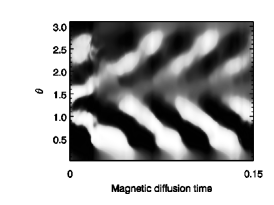
Figure 2: Contour plot of the azimuthally averaged radial magnetic field of model3m versus time and colatitude. The contour plot was normalised by the maximum absolute value at each time step. The grey-scale coding ranges from -1, white, to +1, black.

Moreover, we tested 13 arbitrarily chosen models (see the caption of Table LABEL:tab:2) for kinematic stability and found the dipolar models to be kinematically stable, whereas all multipolar models considered exhibited at least periods of instability. Figure 3 shows as an example the evolution of the kinematically advanced tracer field for model2m and model54d. For the first, the tracer field grows exponentially but it stays stable for the latter although it has been permanently perturbed during the simulation.

Figure 3: Evolution of the energy of the tracer field normalised by the energy of the actual magnetic field for model2m (dashed line) and model54d (solid line).

Figure 4: Relative dipole field strength versus $Ro_{\ell}$ for a sequence of models with $E=3\times 10^{-4}$, $Ra=4Ra_{c}$, $Pm=3$, and $Pr=1$. The meaning of the symbols is as defined in the caption of Fig. 1.

A transition from the dipolar to the multipolar regime can be triggered by a decrease in the rotation rate or the dynamical length scale (possibly associated with a change in the aspect ratio), or an increase in the velocity amplitude. These three quantities influence the local Rossby number directly. In Fig. 4, we show that a transition towards the multipolar regime may also be forced by increasing $N_{\varrho}$. A higher density stratification with all the other parameters fixed causes smaller length scales and larger velocity amplitudes. This leads to an increase of $Ro_{\ell}$ and to a decrease of $f_{\mathrm{dip}}$ at $Ro_{\ell}\approx 0.12$ in Fig. 4.

3.2 Equatorial dipole

An example of a model strongly influenced by an equatorial dipole mode is presented in Fig. 5. A strong mean zonal flow often present in these models seems to be in conflict with the generation of non-axisymmetric fields.

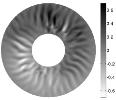
Figure 5: Contour plot (equatorial cut) of the radial magnetic field of model2m at a given time.

Figure 6 demonstrates that the strong equatorial dipole mode of model5m is indeed maintained and rebuilt by the columnar convection and damped by the differential rotation. In Fig. 6 the mean zonal kinetic energy normalised by an arbitrary value (dotted line) and the ratio of the axisymmetric magnetic energy to the total magnetic energy (solid line) are displayed. The action of the mean zonal flow, or more precisely the differential rotation, tends to damp non-axisymmetric components of the magnetic field. Thus, a burst of the mean zonal kinetic energy is followed by a maximum of the axisymmetric and a dip in the non-axisymmetric magnetic energy. Subsequently, the mean zonal flow is quenched by the axisymmetric field, the axisymmetric field decays and the non-axisymmetric field is rebuilt. The interaction between the mean zonal flow and the magnetic field observed in this model is still fairly weak, although the mean zonal flow contributes already $58\%$ to the total kinetic energy. Therefore, the magnetic field of model5m stays on average highly non-axisymmetric. We note that this is very different from the Sun, for instance, where probably an even more efficient differential rotation causes a predominantly axisymmetric large-scale magnetic field (Charbonneau 2010), but also non-axisymmetric stellar magnetic fields were reported (Donati & Landstreet 2009).

Figure 6: Dotted line: axisymmetric kinetic energy of model5m normalised by an arbitrary value; solid line: ratio of axisymmetric to total magnetic energy.

3.3 Discussion

The fundamental cause of the high dipolarity of dynamo models in the low Rossby number regime is an outstanding question. Schrinner et al. (2012) argued for Boussinesq models that cylindrical convection in a spherical fluid domain leads to a characteristic pattern of the axisymmetric toroidal field which eventually results in the clear preference of only one, dipolar eigenmode. The argument relies on the idea that a line of fluid elements moving towards the outer spherical boundary has to shorten and causes a converging flow towards the equatorial plane. The toroidal field is then advected and markedly shaped by this flow component (see also Olson et al. 1999). This advection process could be rigorously identified and quantified as a strong $\gamma-$effect in a corresponding mean-field description (Schrinner et al. 2007, 2012). In addition, the recent finding that the dichotomy of dipolar and multipolar dynamos seems to be absent in convective dynamo simulations in Cartesian geometry (Tilgner 2012) is consistent with this argument and points again to the significance of the underlying symmetry constraints.

What has been said above about Boussinesq models largely applies to anelastic models, too. However, geometrical constraints are somewhat relaxed for a compressible fluid. Therefore, compressibility might damp the advection of the mean toroidal field towards the equatorial plane ($\gamma-$effect) and we hypothesize that this results in at least two specific differences.

First, depending on the density contrast applied, it is more difficult to obtain dipolar solutions for anelastic than for Boussinesq models, even if $Ro_{\ell}<0.12$. However, unlike Gastine et al. (2012), we did not find that dipolar solutions become impossible if $N_{\varrho}$ exceeds a certain threshold. Instead, we observe that for a given $N_{\varrho}$, Ekman and Prandtl number, there seems to exist a critical magnetic Prandtl number for dipolar dynamos. For $E=10^{-4}$ and $Pr=1$, and $N_{\varrho}\geq 1.5$, we found $Pm_{\mathrm{crit}}=2N_{\varrho}-2$, as apparent from Fig. 7. We emphasize again that the results of Fig. 7 depend of course on $E$ and $Pr$; the data of our numerical study indicate that decreasing $E$ and increasing $Pr$ is favorable to dipolar dynamo models.

Second, magnetic field configurations dominated by an equatorial dipole seem to be more easily realized in anelastic than in Boussinesq simulations. For the latter, only a few examples under very specific conditions were reported (Aubert & Wicht 2004; Gissinger et al. 2012). The preference of non-axisymmetric modes is well known from dynamo models based on columnar convection (e.g. Ruediger 1980; Tilgner 1997), it is also the case of the Karlsruhe dynamo experiment (Müller & Stieglitz 2002). This agrees with our reasoning on the importance of the $\gamma-$effect in the axial dipole generation mechanisms (see also Schrinner et al. 2012). Indeed, the $\gamma-$effect vanishes in the above examples, as the geometrical constraints are relaxed.

Figure 7: Magnetic Prandtl number versus $N_{\varrho}$ for models with $E=10^{-4}$ and $Pr=1$ and variable Rayleigh numbers. Filled circles stand for parameters for which dipolar solutions were obtained.

4 Scaling laws

Because of computational limitations, very small length scales and time scales associated with extreme parameter values relevant for planets and stars cannot be resolved in global direct numerical dynamo simulations. Therefore, numerical models are in general not directly comparable to planetary or stellar dynamos. Instead, scaling laws, in particular for the field strength, have been derived from theory and simulations and then extrapolated to realistic parameter regimes (see Christensen 2010, and references therein).

Subsequently, their predictions may be compared with planetary or stellar magnetic-field data obtained from observations (Christensen et al. 2009; Christensen 2010; Davidson 2013). By this consistency test, scaling laws may provide some evidence about the reliability of numerical dynamo models.

Moreover, different scaling laws typically represent different force balances or dynamo mechanisms and their investigation might enable us to better distinguish between different types of dynamo models. It is in particular this second aspect which is of interest in the following. We adopt here the approach by Christensen & Aubert (2006) and derive scaling laws for the field strength, the velocity, the magnetic dissipation time, and the convective heat transport and compare them with previous results from Boussinesq simulations. A similar study was recently published by Yadav et al. (2013b) based on a somewhat different sample of models. Similarities and differences with their findings will be discussed.

Most of the proposed scaling laws are independent of diffusivities, which are thought to be negligible under astrophysical conditions (Christensen 2010). However, present, global dynamo simulations run in parameter regimes where diffusivities still influence the overall dynamics and weak dependencies on the magnetic Prandtl number seem to persist in purely empirically derived scalings (Christensen & Tilgner 2004; Christensen & Aubert 2006; Christensen 2010; Yadav et al. 2013a; Stelzer & Jackson 2013). In this study we do not attempt to resolve this secondary dependence on $Pm$ because the magnetic Prandtl number varies only between 1 and 5 in our sample of models.

4.1 Magnetic field scaling

The magnetic field strength measured in terms of the Lorentz number scales with the available energy flux to the power of approximately $1/3$. We find for the dipolar dynamos of our sample

$$\frac{Lo}{f_{\mathrm{ohm}}^{1/2}}\simeq 1.58\,Ra_{Q}^{0.35}\,,$$ (25)

and for the multipolar models

$$\frac{Lo}{f_{\mathrm{ohm}}^{1/2}}\simeq 1.19\,Ra_{Q}^{0.34}\,.$$ (26)

Except for somewhat larger exponential prefactors, this is in good agreement with previous results from Boussinesq simulations (Christensen 2010; Schrinner et al. 2012; Yadav et al. 2013a) and very similar to the magnetic field scaling given by Yadav et al. (2013b). We note however, that unlike Yadav et al. (2013b), we scale the Lorentz number with the flux based Rayleigh number $Ra_{Q}$ and not directly with the power released by buoyancy forces. Of course, both should be closely related to each other. The same remark applies for the velocity scaling discussed below.

Models on the multipolar branch exhibit lower field strengths compared to their dipolar counterparts. This is not only apparent by the smaller prefactor in the multipolar scaling, but also the dynamo efficiency $f_{\mathrm{ohm}}$ for multipolar models is systematically lower than for the corresponding dipolar ones. The latter indicates that the bistable behaviour for models at $Ro_{\ell}\leq 0.12$ is caused by different dynamo mechanisms. This was already seen in Boussinesq simulations (Schrinner et al. 2012) and later confirmed by Gastine et al. (2012) for anelastic models.

Apart from a few exceptions, the shift between the two scalings in Fig. 8 may serve to separate dipolar from multipolar dynamos. In agreement with Yadav et al. (2013b), we obtained several models with dipole field strengths up to $f_{\mathrm{dip}}\approx 0.5$ which nevertheless clearly follow the multipolar scaling and belong to the multipolar class of dynamos.

Figure 8: Lorentz number compensated by $f_{\mathrm{ohm}}$ versus the flux-based Rayleigh number for our sample of models. Filled symbols correspond to dipolar models, open symbols are multipolar models and the symbol shape indicates $N_{\rho}$ as explained in the caption of Fig. 1.

4.2 Velocity scaling

There is an ongoing discussion about the velocity scaling in dynamo models (Christensen 2010; Davidson 2013; Yadav et al. 2013b). It is probably not surprising that the velocity measured in terms of the Rossby number scales with the flux based Rayleigh number, but the correct exponent and its theoretical justification is debated. The lower bound is set by the assumption of a balance between inertia and buoyancy forces (mixing length balance), which leads to an exponent of $1/3$ (Christensen 2010). If however, the predominant force balance is assumed to be between the Lorentz force, the buoyancy and the Coriolis force (MAC-balance) the exponent is closer to $1/2$ (Christensen 2010; Davidson 2013). As most previous studies (Christensen & Aubert 2006; Christensen 2010; Yadav et al. 2013a; Stelzer & Jackson 2013; Yadav et al. 2013b) we obtained for our sample of models an exponent in between these two values,

$$Ro=1.66\,Ra_{Q}^{0.42}\,.$$ (27)

The scatter in Fig. 9 is considerable, but the standard error is of the same order as for Boussinesq models with stress-free mechanical boundary conditions (Yadav et al. 2013a). Compressible effects do not seem to deteriorate the scaling.

Figure 9: Rossby number versus the flux-based Rayleigh number for our sample of models.

However, as in Yadav et al. (2013b), we are not able to distinguish between dipolar and multipolar models in our velocity scaling contrary to what has been previously reported by Yadav et al. (2013a) for Boussinesq models.

4.3 Scaling of Ohmic dissipation time

The scaling of magnetic dissipation time,

$$\tau_{\mathrm{diss}}=E_{M}/D=\ell_{B}^{2}/\eta\,,$$ (28)

is used to evaluate the characteristic length scale $\ell_{B}$ of the magnetic field. Christensen & Tilgner (2004) originally identified a linear dependence of $\tau_{\mathrm{diss}}$ on the inverse Rossby number provided that time is measured in units of $\Omega^{-1}$. Their finding was supported by dipole-dominated Boussinesq models with no-slip mechanical boundary conditions and the evaluation of the Ohmic dissipation time in the Karlsruhe dynamo experiment. The best fit for our data points in Fig. 10, however, gives an exponent with a significantly lower absolute value,

$$\tau_{\mathrm{diss}}=0.75\,Ro^{-0.76}\,.$$ (29)

An almost identical result was found by Yadav et al. (2013b) from their somewhat more diverse and scattered data set. Apparently, the application of stress-free boundary conditions and maybe also compressible effects flatten the slope of $\tau_{\mathrm{diss}}$ as a function of the Rossby number. Moreover, it would seem plausible that $\tau_{\mathrm{diss}}$ followed different scaling relations for dipolar and multipolar models. Indeed, for bistable pairs, the dissipation time is systematically larger for dipolar than for multipolar models. However, separate least square fits for all dipolar and all multipolar models of our sample lead to very similar results.

Figure 10: Ohmic dissipation time versus Rossby number for all models considered in this study.

4.4 Nusselt number scaling

The convective heat transport in dynamo models is very sensitive to rotation and depends to a much lower degree on the magnetic field, boundary conditions or the geometry of the fluid domain (Christensen 2002; Christensen & Aubert 2006; Aurnou 2007; Schmitz & Tilgner 2009; Busse & Simitev 2011; Gastine & Wicht 2012; Yadav et al. 2013a; Stelzer & Jackson 2013). The power law for the Nusselt number inferred from Fig. 11,

$$Nu^{\star}=0.25\,Ra_{Q}^{0.59}\,,$$ (30)

is consistent with previous results and confirms this finding also for anelastic dynamo models; the exponent of $0.59$ is very close to the value of $5/9$ established by the above mentioned references. However, the scaling is somewhat more scattered than for Boussinesq models (Yadav et al. 2013a). We excluded in a test all models for which convection is only marginaly above the onset ($Nu^{\star}<2$), but this reselection of models did not improve the quality of the fit.

Figure 11: Nusselt number versus the flux-based Rayleigh number for our sample of models.

4.5 Discussion

Table 1: Scaling laws for anelastic and Boussinesq models. Results for Boussinesq models were taken from Yadav et al. (2013a) (see also Schrinner et al. 2012).

Scaling	Anelastic			Boussinesq
	c	x	$\sigma$	c	x	$\sigma$
$Lo/f_{\mathrm{ohm}}^{1/2}=c\,Ra_{Q}^{x}$	1.58	0.35	0.017	1.08	0.37	0.017
multipolar branch	1.19	0.34	0.067	0.65	0.35	0.006
$Ro=c\,Ra_{Q}^{x}$	1.66	0.42	0.025	0.73	0.39	0.013
				1.79	0.44	0.010
$\tau_{\mathrm{diss}}=c\,Ro^{-x}$	0.75	0.76	0.024	–	0.8	–
$Nu=c\,Ra_{Q}^{x}$	0.25	0.59	0.032	0.06	0.52	0.004

In an overall view, the scaling relations for Boussinesq and anelastic models are very similar (see Table 1). Beyond that, there is no obvious effect of compressibility on the scaling results and they might be even considered as consistent irrespective of the density stratification of the underlying models (Yadav et al. 2013b). However, the reason for the good agreement could be that the flux-based scaling laws are insensitive to different physical conditions. Using the example of the magnetic field scaling, we argue in the following that differences in the dynamo processes might not be visible in the scaling relation and some caution is needed in generalizing results from Boussinesq simulations.

If the magnetic energy density follows a simple power law in terms of the convective energy flux an exponent of $2/3$ is already required for dimensional reasons (e.g. Christensen 2010). Moreover, the flux-based scaling law for the magnetic field is composed of the scalings for the velocity and the magnetic dissipation time. By definition, we have $E_{M}\sim f_{\mathrm{ohm}}\,\tau_{\mathrm{diss}}\,P$ and with $Ro\sim P^{\alpha}$ and $\tau_{\mathrm{diss}}\sim Ro^{\beta}$, we find $E_{M}\sim f_{\mathrm{ohm}}\,P\,P^{\alpha\beta}$. Dimensional arguments require $\alpha\,\beta=-1/3$ which establishes relations (25) and (26). Whereas the exponent in the flux-based scaling law for the magnetic field is fix, $\alpha$ and $\beta$ are to some extend variable and may change according to the specific physical conditions. This reflects the outcome of more and more extended parameter studies: the exponent of $1/3$ in the magnetic-field scaling is reliably reproduced but the values for $\alpha$ and $\beta$ seem to be less certain and are under debate.

In addition, scaling relations (25) and (26) require that the field strength, measured by $Lo$, is compensated by the square root of $f_{\mathrm{ohm}}$ (interpreted as dynamo efficiency in Schrinner 2013). However, $f_{\mathrm{ohm}}$ probably is a complicated function of several control parameters and might depend strongly on the specific physical conditions. The often made assumption that $f_{\mathrm{ohm}}\rightarrow 1$ for $Pm\ll 1$ (e.g. Davidson 2013) is probably too simple. For example, Schrinner (2013) demonstrated recently that $f_{\mathrm{ohm}}$ in dynamo models might depend strongly on the rotation rate. The dynamo efficiency dropped by two orders of magnitude as the rotation rate of these models was decreased. A further counterexample could be the solar dynamo. Independent estimates result in $f_{\mathrm{ohm}}\sim O(10^{-3})$ (Schrinner 2013; Rempel 2006) although the magnetic Prandtl number is thought to be much smaller than one in the solar interior. In other words, the flux based scaling laws probably do not discriminate between different types of dynamos because differences in the field strength are absorbed by changes in $f_{\mathrm{ohm}}$.

5 Conclusions

Our study revealed a number of similarities between Boussinesq and anelastic dynamo models. The dichotomy between dipolar and multipolar models seems to extend to anelastic models, and the flux-based scaling laws originally proposed for Boussineq models appear to hold similarly for models in the anelastic approximation. Thus, large scale, dipolar magnetic fields for both types of models can only be produced if rotation is important (as measured by the local Rossby number) and the magnetic field strength is directly related to the energy flux via (25) and (26) (see Fig. 8).

However, we also pointed out some significant differences between Boussinesq and anelastic dynamo simulations. Magnetic field configurations with a significant equatorial dipole contribution are less typical for Boussinesq than for anelastic models. Moreover, a large density stratification in anelastic models may inhibit the generation of magnetic fields dominated by an axial dipole. The above claimed consistency of the scalings for Boussinesq and anelastic simulations partly relies on the very general formulation of the flux-based scaling laws and does not necessarily imply similar dynamo processes. We also stress that the assumption of a radially varying conductivity may introduce additional effects which were not examined here. Whereas Yadav et al. (2013b) obtained very similar scaling laws for models with variable conductivities, Duarte et al. (2013) reported that the field topology of some models depends on the radial conductivity profile. A mean-field analysis (Schrinner et al. 2007; Schrinner 2011) of numerical dynamo models in the anelastic approximation might give more detailed insight in relevant dynamo processes and is envisaged for a future study.

Appendix A Benchmark results

Table 2: Hydrodynamic benchmark ($E=10^{-3},\,N_{\varrho}=5,\,\chi=0.35,\,Ra=3.52\times 10^{5},\,Pr=1,\,n=2$)

Code	PaRoDy	Leeds
K.E.	81.85	81.86
Zonal K.E.	9.388	9.377
Meridional K.E.	0.02198	0.02202
Luminosity	4.170	4.199
$v_{\phi}$ at $v_{r}=0$	0.8618	0.8618
$S$ at $u_{r}=0$	0.9334	0.9330
Resolution	$288\,\times\,192\times\,384$	$128\,\times\,192\times\,384$
Timestep	$5\times 10^{-6}$	$2.5\times 10^{-6}$

Table 3: The steady dynamo benchmark ( $E=2\times 10^{-3},\,N_{\varrho}=3,\,\chi=0.35,\,Ra=8.00\times 10^{4},\,Pr=1,\,Pm=50,\,n=2$)

Code	PaRoDy	Leeds
K.E.	$4.189\times 10^{6}$	$4.194\times 10^{5}$
Zonal K.E.	$5.993\times 10^{4}$	$6.018\times 10^{4}$
Meridional K.E.	52.98	53.02
M.E.	$3.216\times 10^{5}$	$3.202\times 10^{5}$
Zonal M.E.	$2.424\times 10^{5}$	$2.412\times 10^{5}$
Meridional M.E.	$1.704\times 10^{5}$	$1.697\times 10^{4}$
Luminosity	11.48	11.50
$v_{\phi}$ at $v_{r}=0$	-91.84	-91.78
$B_{\theta}$ at $v_{r}=0$	$\pm 0.0343$	$\pm 0.03395$
$S$ at $u_{r}=0$	0.7864	0.7865
Resolution	$288\,\times\,126\times\,252$	$128\,\times\,144\times\,252$
Timestep	$5\times 10^{-7}$	$10^{-6}$

Table 4: The unsteady dynamo benchmark ($E=5\times 10^{-5},\,N_{\varrho}=3,\,\chi=0.35,\,Ra=2.50\times 10^{7},\,Pr=2,\,Pm=2,\,n=2$)

Code	PaRoDy	Leeds
K.E.	$2.33\times 10^{5}$	$2.32\times 10^{5}$
Zonal K.E.	$1.38\times 10^{4}$	$1.36\times 10^{4}$
Meridional K.E.	111	105
M.E.	$2.41\times 10^{5}$	$2.42\times 10^{5}$
Zonal M.E.	$9.35\times 10^{3}$	$9.45\times 10^{3}$
Meridional M.E.	$2.10\times 10^{4}$	$2.13\times 10^{4}$
Luminosity	42.4	42.5
Resolution	$288\,\times\,255\times\,510$	$96\,\times\,288\times\,576$
Timestep	$5\times 10^{-7}$	$3\times 10^{-6}$

Appendix B Critical Rayleigh numbers for the onset of convection

Table 5: Overview of the critical Rayleigh numbers and the corresponding critical azimuthal wavenumbers for the onset of convection determined as explained in Jones et al. (2009).

$E$	$Pr$	$N_{\varrho}$	$\chi$	$Ra_{c}$	$m_{c}$
$3\times 10^{-5}$	$1$	$2.0$	$0.35$	$6.79\times 10^{6}$	$24$
$1\times 10^{-4}$	$1$	$0.5$	$0.35$	$3.34\times 10^{5}$	$10$
$1\times 10^{-4}$	$1$	$1.0$	$0.35$	$5.67\times 10^{5}$	$12$
$1\times 10^{-4}$	$1$	$1.5$	$0.35$	$9.25\times 10^{5}$	$14$
$1\times 10^{-4}$	$1$	$1.7$	$0.35$	$1.09\times 10^{6}$	$15$
$1\times 10^{-4}$	$1$	$2.0$	$0.35$	$1.43\times 10^{6}$	$16$
$1\times 10^{-4}$	$1$	$2.5$	$0.35$	$2.18\times 10^{6}$	$19$
$1\times 10^{-4}$	$1$	$3.0$	$0.35$	$3.02\times 10^{6}$	$29$
$1\times 10^{-4}$	$1$	$3.5$	$0.35$	$3.62\times 10^{6}$	$37$
$1\times 10^{-4}$	$1$	$4.0$	$0.35$	$4.09\times 10^{6}$	$43$
$1\times 10^{-4}$	$2$	$3.0$	$0.35$	$7.48\times 10^{6}$	$33$
$1\times 10^{-4}$	$1$	$2.0$	$0.55$	$5.35\times 10^{6}$	$42$
$3\times 10^{-4}$	$1$	$0.5$	$0.35$	$9.66\times 10^{4}$	$7$
$3\times 10^{-4}$	$1$	$1.0$	$0.35$	$1.52\times 10^{5}$	$9$
$3\times 10^{-4}$	$1$	$1.5$	$0.35$	$2.32\times 10^{5}$	$10$
$3\times 10^{-4}$	$1$	$2.0$	$0.35$	$3.51\times 10^{5}$	$12$
$3\times 10^{-4}$	$1$	$2.5$	$0.35$	$5.19\times 10^{5}$	$14$
$3\times 10^{-4}$	$1$	$3.0$	$0.35$	$7.12\times 10^{5}$	$19$
$3\times 10^{-4}$	$1$	$3.5$	$0.35$	$8.71\times 10^{5}$	$25$
$3\times 10^{-4}$	$1$	$2.0$	$0.45$	$6.83\times 10^{5}$	$18$
$3\times 10^{-4}$	$1$	$2.0$	$0.55$	$1.26\times 10^{6}$	$28$
$3\times 10^{-4}$	$2$	$3.0$	$0.35$	$8.90\times 10^{5}$	$22$
$1\times 10^{-3}$	$1$	$2.0$	$0.35$	$7.70\times 10^{4}$	$8$
$2\times 10^{-3}$	$1$	$2.5$	$0.35$	$4.60\times 10^{4}$	$7$

Appendix C Numerical models

htbp]

Table 6: Overview of the simulations carried out, ordered with respect to their local Rossby number.

Model	$E$	$Ra$	$Pm$	$Pr$	$\chi$	$N_{\varrho}$	$Ro_{\ell}$	$Rm$	$Lo$	$f_{\mathrm{dip}}$	$f_{\mathrm{ohm}}$	$Nu$
1m	$1\times 10^{-4}$	$5.00\times 10^{6}$	2.0	2	0.35	3.0	$1.54\times 10^{-2}$	34	$1.10\times 10^{-3}$	0.07	0.05	1.3
2m	$1\times 10^{-4}$	$5.00\times 10^{6}$	3.0	2	0.35	3.0	$1.69\times 10^{-2}$	57	$2.06\times 10^{-3}$	0.55	0.09	1.4
3m	$1\times 10^{-4}$	$5.00\times 10^{6}$	4.0	2	0.35	3.0	$1.80\times 10^{-2}$	78	$2.35\times 10^{-3}$	0.26	0.12	1.4
4m	$1\times 10^{-4}$	$5.00\times 10^{6}$	5.0	2	0.35	3.0	$1.80\times 10^{-2}$	95	$2.21\times 10^{-3}$	0.28	0.11	1.4
5m	$1\times 10^{-4}$	$2.00\times 10^{6}$	1.0	1	0.35	0.5	$2.52\times 10^{-2}$	65	$2.16\times 10^{-3}$	0.43	0.08	1.5
6d	$2\times 10^{-3}$	$8.00\times 10^{4}$	50	1	0.35	3.0	$2.71\times 10^{-2}$	240	$8.38\times 10^{-3}$	0.83	0.01	1.1
7d	$5\times 10^{-5}$	$1.50\times 10^{7}$	2.0	1	0.35	1.5	$2.72\times 10^{-2}$	128	$3.89\times 10^{-3}$	0.79	0.31	1.6
7m	$5\times 10^{-5}$	$1.50\times 10^{7}$	2.0	1	0.35	1.5	$2.51\times 10^{-2}$	164	$2.84\times 10^{-3}$	0.20	0.22	1.6
8m	$1\times 10^{-4}$	$2.00\times 10^{6}$	1.5	1	0.35	0.5	$2.77\times 10^{-2}$	83	$3.08\times 10^{-3}$	0.39	0.13	1.7
9d	$3\times 10^{-4}$	$4.00\times 10^{5}$	3.0	1	0.35	0.5	$2.94\times 10^{-2}$	78	$8.78\times 10^{-3}$	0.85	0.28	1.5
10d	$1\times 10^{-4}$	$7.64\times 10^{5}$	2.0	1	0.60	1.5	$3.19\times 10^{-2}$	44	$2.89\times 10^{-3}$	0.78	0.14	1.2
10m	$1\times 10^{-4}$	$7.64\times 10^{5}$	2.0	1	0.60	1.5	$3.12\times 10^{-2}$	42	$2.03\times 10^{-3}$	0.35	0.11	1.2
11d	$1\times 10^{-4}$	$2.78\times 10^{6}$	2.0	1	0.35	1.5	$3.39\times 10^{-2}$	104	$5.72\times 10^{-3}$	0.78	0.26	1.6
12d	$3\times 10^{-5}$	$1.96\times 10^{7}$	2.0	1	0.35	2.0	$3.39\times 10^{-2}$	213	$3.87\times 10^{-3}$	0.68	0.32	2.1
12m	$3\times 10^{-5}$	$1.96\times 10^{7}$	2.0	1	0.35	2.0	$3.33\times 10^{-2}$	207	$3.02\times 10^{-3}$	0.24	0.23	2.0
13d	$1\times 10^{-4}$	$6.14\times 10^{6}$	2.0	1	0.60	1.0	$3.41\times 10^{-2}$	49	$2.75\times 10^{-3}$	0.68	0.12	1.2
13m	$1\times 10^{-4}$	$6.14\times 10^{6}$	2.0	1	0.60	1.0	$3.44\times 10^{-2}$	49	$2.32\times 10^{-3}$	0.05	0.12	1.2
14m	$1\times 10^{-4}$	$2.50\times 10^{6}$	1.5	1	0.35	0.5	$3.51\times 10^{-2}$	106	$4.59\times 10^{-3}$	0.49	0.19	2.0
15d	$1\times 10^{-4}$	$4.01\times 10^{6}$	3.0	1	0.35	2.5	$3.76\times 10^{-2}$	144	$6.74\times 10^{-3}$	0.52	0.24	1.7
15m	$1\times 10^{-4}$	$4,01\times 10^{6}$	3.0	1	0.35	2.5	$4.51\times 10^{-2}$	182	$6.48\times 10^{-3}$	0.47	0.23	1.7
16d	$1\times 10^{-4}$	$5,00\times 10^{6}$	4.0	1	0.35	3.0	$3.76\times 10^{-2}$	182	$6.64\times 10^{-3}$	0.47	0.23	1.5
17d	$1\times 10^{-4}$	$3.00\times 10^{6}$	2.0	1	0.35	0.5	$3.90\times 10^{-2}$	148	$8.15\times 10^{-3}$	0.75	0.37	2.3
18d	$1\times 10^{-4}$	$3.01\times 10^{6}$	1.5	1	0.35	0.5	$4.00\times 10^{-2}$	112	$7.83\times 10^{-3}$	0.87	0.35	2.3
18m	$1\times 10^{-4}$	$3.01\times 10^{6}$	1.5	1	0.35	0.5	$4.32\times 10^{-2}$	127	$6.09\times 10^{-3}$	0.39	0.23	2.3
19m	$5\times 10^{-5}$	$2.52\times 10^{7}$	2.0	2	0.35	3.0	$4.46\times 10^{-2}$	176	$4.62\times 10^{-3}$	0.30	0.26	3.4
20d	$1\times 10^{-4}$	$3.40\times 10^{6}$	1.0	1	0.35	1.0	$4.71\times 10^{-2}$	80	$8.55\times 10^{-3}$	0.86	0.37	2.4
20m	$1\times 10^{-4}$	$3.40\times 10^{6}$	1.0	1	0.35	1.0	$4.62\times 10^{-2}$	97	$5.93\times 10^{-3}$	0.32	0.24	2.3
21d	$3\times 10^{-4}$	$6.08\times 10^{5}$	3.0	1	0.35	1.0	$4.86\times 10^{-2}$	115	$1.27\times 10^{-2}$	0.64	0.31	1.9
22d	$1\times 10^{-4}$	$3.40\times 10^{6}$	1.5	1	0.35	1.0	$4.88\times 10^{-2}$	124	$8.76\times 10^{-3}$	0.75	0.35	2.4
22m	$1\times 10^{-4}$	$3.40\times 10^{6}$	1.5	1	0.35	1.0	$4.78\times 10^{-2}$	132	$6.62\times 10^{-3}$	0.39	0.25	2.3
23m	$1\times 10^{-4}$	$1.00\times 10^{7}$	3.0	2	0.35	3.0	$5.13\times 10^{-2}$	203	$6.26\times 10^{-3}$	0.14	0.19	3.6
24d	$1\times 10^{-4}$	$4.00\times 10^{6}$	2.0	1	0.35	1.5	$5.30\times 10^{-2}$	170	$8.37\times 10^{-3}$	0.69	0.33	2.6
25d	$3\times 10^{-4}$	$1.00\times 10^{6}$	3.0	1	0.35	2.5	$5.36\times 10^{-2}$	226	$1.17\times 10^{-2}$	0.75	0.21	1.6
26m	$1\times 10^{-4}$	$1.14\times 10^{7}$	2.0	1	0.60	2.0	$5.38\times 10^{-2}$	70	$3.41\times 10^{-3}$	0.24	0.14	1.4
27m	$1\times 10^{-4}$	$1.00\times 10^{7}$	3.0	2	0.35	3.0	$5.46\times 10^{-2}$	205	$6.24\times 10^{-3}$	0.21	0.19	3.6
28d	$3\times 10^{-4}$	$8.00\times 10^{5}$	3.0	1	0.35	0.5	$6.06\times 10^{-2}$	161	$2.14\times 10^{-2}$	0.76	0.41	2.5
29d	$1\times 10^{-4}$	$5.00\times 10^{6}$	3.0	1	0.35	2.0	$6.10\times 10^{-2}$	270	$1.00\times 10^{-2}$	0.61	0.36	2.6
30m	$1\times 10^{-4}$	$5.00\times 10^{6}$	1.0	1	0.35	1.7	$6.50\times 10^{-2}$	100	$8.06\times 10^{-3}$	0.5	0.26	2.6
31d	$1\times 10^{-4}$	$5.00\times 10^{6}$	1.0	1	0.35	0.5	$6.70\times 10^{-2}$	126	$1.41\times 10^{-2}$	0.83	0.48	3.8
31m	$1\times 10^{-4}$	$5.00\times 10^{6}$	1.0	1	0.35	0.5	$7.10\times 10^{-2}$	140	$1.05\times 10^{-2}$	0.45	0.34	3.8
32d	$1\times 10^{-4}$	$5.00\times 10^{6}$	2.0	1	0.35	1.5	$6.70\times 10^{-2}$	220	$1.16\times 10^{-2}$	0.65	0.40	3.2
33d	$1\times 10^{-4}$	$5.00\times 10^{6}$	3.0	1	0.35	1.7	$6.70\times 10^{-2}$	300	$1.08\times 10^{-2}$	0.63	0.37	2.9
34d	$1\times 10^{-4}$	$5.00\times 10^{6}$	2.0	1	0.35	1.7	$6.80\times 10^{-2}$	200	$1.07\times 10^{-2}$	0.67	0.35	3.0
35d	$3\times 10^{-4}$	$6.08\times 10^{5}$	3.0	1	0.35	1.5	$6.99\times 10^{-2}$	160	$1.78\times 10^{-2}$	0.59	0.34	2.3
36d	$1\times 10^{-4}$	$8.00\times 10^{6}$	4.0	1	0.35	3.0	$7.00\times 10^{-2}$	380	$1.41\times 10^{-2}$	0.62	0.40	2.9
37d	$3\times 10^{-4}$	$1.05\times 10^{6}$	3.0	1	0.35	2.0	$7.21\times 10^{-2}$	152	$1.60\times 10^{-2}$	0.67	0.31	2.1
38m	$1\times 10^{-4}$	$1.20\times 10^{7}$	5.0	1	0.35	4.0	$7.22\times 10^{-2}$	458	$1.15\times 10^{-2}$	0.19	0.32	2.6
39d	$1\times 10^{-4}$	$5.55\times 10^{6}$	2.0	1	0.35	1.5	$7.40\times 10^{-2}$	247	$1.52\times 10^{-2}$	0.63	0.49	3.6
40d	$1\times 10^{-4}$	$6.00\times 10^{6}$	1.0	1	0.35	0.5	$8.00\times 10^{-2}$	150	$1.64\times 10^{-2}$	0.82	0.49	4.7
41d	$1\times 10^{-4}$	$1.00\times 10^{7}$	5.0	1	0.35	3.5	$8.20\times 10^{-2}$	500	$1.23\times 10^{-2}$	0.63	0.33	3.2
42d	$1\times 10^{-4}$	$6.50\times 10^{6}$	1.0	1	0.35	1.5	$8.80\times 10^{-2}$	150	$1.64\times 10^{-2}$	0.77	0.45	4.6
43d	$1\times 10^{-4}$	$7.00\times 10^{6}$	2.0	1	0.35	2.0	$8.80\times 10^{-2}$	280	$1.64\times 10^{-2}$	0.66	0.46	4.3
44m	$1\times 10^{-4}$	$7.00\times 10^{6}$	1.0	1	0.35	2.0	$9.05\times 10^{-2}$	140	$1.18\times 10^{-2}$	0.04	0.34	3.7
45d	$1\times 10^{-3}$	$2.50\times 10^{5}$	3.0	1	0.35	2.5	$9.07\times 10^{-2}$	87	$2.76\times 10^{-2}$	0.82	0.23	1.7
45m	$1\times 10^{-3}$	$2.50\times 10^{5}$	3.0	1	0.35	2.5	$6.35\times 10^{-2}$	86	$2.17\times 10^{-2}$	0.31	0.19	1.6
46m	$1\times 10^{-4}$	$6.00\times 10^{6}$	1.0	1	0.35	0.5	$9.20\times 10^{-2}$	170	$1.26\times 10^{-2}$	0.52	0.35	4.6
47d	$3\times 10^{-4}$	$1.50\times 10^{6}$	3.0	1	0.35	2.5	$9.35\times 10^{-2}$	191	$2.29\times 10^{-2}$	0.59	0.37	2.6
47m	$3\times 10^{-4}$	$1.50\times 10^{6}$	3.0	1	0.35	2.5	$8.67\times 10^{-2}$	234	$1.67\times 10^{-2}$	0.39	0.22	2.2
48m	$3\times 10^{-4}$	$2.52\times 10^{6}$	3.0	1	0.55	2.0	$9.81\times 10^{-2}$	112	$1.12\times 10^{-2}$	0.27	0.21	1.8
49d	$3\times 10^{-4}$	$1.40\times 10^{6}$	3.0	1	0.35	2.0	$1.01\times 10^{-1}$	221	$2.47\times 10^{-2}$	0.51	0.36	2.8
50d	$3\times 10^{-4}$	$1.50\times 10^{6}$	3.0	1	0.35	1.5	$1.09\times 10^{-1}$	265	$3.18\times 10^{-2}$	0.67	0.45	3.7
51d	$1\times 10^{-4}$	$8.00\times 10^{6}$	1.0	1	0.35	1.5	$1.10\times 10^{-1}$	190	$1.97\times 10^{-2}$	0.77	0.49	5.8
52d	$1\times 10^{-4}$	$1.52\times 10^{7}$	3.0	1	0.55	2.0	$1.13\times 10^{-1}$	369	$2.10\times 10^{-2}$	0.64	0.54	4.3
53d	$3\times 10^{-4}$	$2.05\times 10^{6}$	3.0	1	0.45	2.0	$1.14\times 10^{-1}$	186	$2.27\times 10^{-2}$	0.60	0.35	2.6
54d	$1\times 10^{-3}$	$3.00\times 10^{5}$	3.0	1	0.35	2.5	$1.19\times 10^{-1}$	108	$4.14\times 10^{-2}$	0.74	0.33	2.2
54m	$1\times 10^{-3}$	$3.00\times 10^{5}$	3.0	1	0.35	2.5	$1.13\times 10^{-1}$	114	$2.97\times 10^{-2}$	0.27	0.28	2.1
55d	$3\times 10^{-4}$	$2.00\times 10^{6}$	3.0	1	0.35	2.5	$1.22\times 10^{-1}$	277	$2.91\times 10^{-2}$	0.56	0.38	3.6
56d	$3\times 10^{-4}$	$2.39\times 10^{6}$	3.0	1	0.45	2.0	$1.29\times 10^{-1}$	215	$2.73\times 10^{-2}$	0.59	0.42	3.1
56m	$3\times 10^{-4}$	$2.39\times 10^{6}$	3.0	1	0.45	2.0	$1.25\times 10^{-1}$	243	$2.05\times 10^{-2}$	0.32	0.29	3.3
57m	$3\times 10^{-4}$	$2.08\times 10^{6}$	3.0	1	0.35	2.5	$1.30\times 10^{-1}$	291	$2.71\times 10^{-2}$	0.32	0.36	3.7
58m	$3\times 10^{-4}$	$2.50\times 10^{6}$	3.0	1	0.35	3.0	$1.28\times 10^{-1}$	272	$2.58\times 10^{-2}$	0.26	0.35	3.4
59m	$3\times 10^{-4}$	$5.00\times 10^{5}$	2.0	2	0.35	3.0	$1.34\times 10^{-1}$	191	$1.98\times 10^{-2}$	0.28	0.29	5.4
60m	$3\times 10^{-4}$	$3.50\times 10^{6}$	3.0	1	0.35	3.5	$1.41\times 10^{-1}$	294	$2.58\times 10^{-2}$	0.17	0.34	3.6
61m	$3\times 10^{-4}$	$2.85\times 10^{6}$	3.0	1	0.35	3.0	$1.43\times 10^{-1}$	314	$2.79\times 10^{-2}$	0.21	0.36	3.8
62m	$3\times 10^{-4}$	$2.50\times 10^{6}$	3.0	1	0.35	2.5	$1.47\times 10^{-1}$	342	$3.15\times 10^{-2}$	0.28	0.39	4.2
63m	$1\times 10^{-4}$	$1.10\times 10^{7}$	1.0	1	0.35	2.5	$1.50\times 10^{-1}$	240	$1.58\times 10^{-2}$	0.28	0.37	5.2
64m	$3\times 10^{-4}$	$3.78\times 10^{6}$	3.0	1	0.55	2.0	$1.52\times 10^{-1}$	200	$1.92\times 10^{-2}$	0.17	0.31	2.7
65m	$1\times 10^{-3}$	$4.00\times 10^{5}$	3.0	1	0.35	2.5	$1.66\times 10^{-1}$	162	$4.39\times 10^{-2}$	0.26	0.26	2.6
66m	$2\times 10^{-3}$	$2.00\times 10^{5}$	3.0	1	0.35	2.5	$2.18\times 10^{-1}$	150	$4.66\times 10^{-2}$	0.19	0.17	2.6

Table 6: continued.