A state-constrained differential game
arising in optimal portfolio liquidation

Abstract

We consider $n$ risk-averse agents who compete for liquidity in an Almgren–Chriss market impact model. Mathematically, this situation can be described by a Nash equilibrium for a certain linear-quadratic differential game with state constraints. The state constraints enter the problem as terminal boundary conditions for finite and infinite time horizons. We prove existence and uniqueness of Nash equilibria and give closed-form solutions in some special cases. We also analyze qualitative properties of the equilibrium strategies and provide corresponding financial interpretations.

Keywords: Optimal portfolio liquidation, optimal trade execution, illiquid markets, differential game with state constraints

1 Introduction

In this paper, we analyze a state-constrained differential game that arises for risk-averse agents aiming to liquidate a given asset position by a given time $T>0$. Agents face both price impact and volatility risk. For each agent, there is hence a tradeoff between slow trading so as to reduce transaction costs from price impact and fast liquidation in view of volatility risk. Beginning with Bertsimas and Lo (1998) and Almgren and Chriss (2000), a large numbers of papers have studied the corresponding single-agent optimization problems in various settings; see Lehalle (2013) and Gatheral and Schied (2013) for recent overviews and more complete lists of references. The problem becomes even more interesting when considering not just one, but $n$ agents who are aware of each others initial positions, a situation that is not unlikely to occur in reality; see Carlin et al. (2007) and Schöneborn and Schied (2009). Together with Brunnermeier and Pedersen (2005), these two papers were among the first to consider a game theoretic approach, but only study open-loop Nash equilibria for risk-neutral agents using deterministic strategies. Moallemi et al. (2012) extend the analysis to a model with asymmetric information. Carmona and Yang (2011) use numerical simulations to study a system of coupled HJB equations arising from a closed-loop Nash equilibrium for two utility-maximizing agents. Lachapelle et al. (2013) apply mean-field games to model the price formation process in the presence of high-frequency traders. A two-player Nash equilibrium in a market impact model with exponentially decaying transient price impact is analyzed in Schied and Zhang (2013).

Here, we consider agents maximizing a mean-variance functional in a continuous-time Almgren and Chriss (2000) framework, which is a common setup for portfolio liquidation. It leads to a linear-quadratic differential game, which has the interesting additional feature of a terminal state constraint arising from the liquidation constraint on the portfolio. This state constraint leads to two-point boundary problems in place of the usual initial value problems connected with unconstrained differential games. Aside from the financial interpretation of our results, this paper thus also provides a natural case study for a class state-constrained differential games.

Our main results establish existence and uniqueness for the corresponding Nash equilibria with both finite and infinite time horizon. In several cases, we can also give closed-form solutions for the equilibrium strategies. These formulas enable us to discuss some qualitative properties of the Nash equilibrium. Some of these properties are surprising, as they show that certain monotonicity properties that are discussed in the finance literature may break down under certain market conditions. See Lebedeva et al. (2012) for discussions and for an empirical analysis of a large data set of portfolio liquidations of large investors.

The paper is organized as follows. In Section 2.1, we recall some background material on portfolio liquidation in the Almgren–Chriss framework. Existence, uniqueness, and representation results for Nash equilibria with finite time horizon are stated in Section 2.2. Section 2.3 contains a discussion of the qualitative properties of the corresponding two-player Nash equilibrium. Nash equilibria with infinite time horizon are discussed in Section 3. All proofs can be found in Section 4.

2 Nash equilibrium with finite time horizon

2.1 Background

We consider a standard continuous-time Almgren and Chriss (2000) framework for investors who are active over a fixed time period $[0,T]$. An investor may hold an initial position of $x$ shares and is required to close this position by time $T$. The information flow available to an investor is modeled by a filtration $({\mathscr{F}}_{t})_{t\geq 0}$ on a given probability space $(\Omega,{\mathscr{F}},{\mathbb{P}})$. The trading strategy employed by the investor is denoted by $X=(X(t))_{t\in[0,T]}$. It needs to satisfy the following conditions of admissibility:
$\bullet$ $X$ satisfies the liquidation constraint $X(T)=0$;
$\bullet$ $X$ is adapted to the filtration $({\mathscr{F}}_{t})_{t\geq 0}$;
$\bullet$ $X$ is absolutely continuous in the sense that there exists a progressively measurable process $(\dot{X}(t))_{t\in[0,T]}$ such that for all $\omega\in\Omega$, $\int_{0}^{T}(\dot{X}(t,\omega))^{2}\,dt<\infty$ and

$$X(t,\omega)=X(0,\omega)+\int_{0}^{t}\dot{X}(s,\omega)\,ds,\qquad t\in[0,T];$$

$\bullet$ there exists a constant $c\geq 0$ such that $|X(t,\omega)|\leq c$ for all $t$ and $\omega$.
The class of all strategies that are admissible in this sense and satisfy $X(0)=x$ for given $x\in\mathbb{R}$ will be denoted by ${\mathscr{X}}(x,T)$. Let us also introduce the subclass ${\mathscr{X}}_{\text{det}}(x,T)$ of all strategies in ${\mathscr{X}}(x,T)$ that are deterministic in the sense that they do not depend on $\omega$. The ‘unaffected price process’ $S^{0}$ will describe the fluctuations of asset prices perceived by an investor who has no inside information on large trades carried out by other market participants during the time interval $[0,T]$. In the Almgren–Chriss model, it is usually assumed that $S^{0}$ follows a Bachelier model. Here we are sometimes also going to allow for an extra drift to describe current price trends. Thus,

$$S^{0}(t)=S_{0}+\sigma W(t)+\int_{0}^{t}b(s)\,ds,$$

where $S_{0}$ is a constant, $W$ is a standard Brownian motion, $\sigma\geq 0$, and $b$ is deterministic and continuous.

When an investor is using a strategy $X\in{\mathscr{X}}(x,T)$, the strategy $X$ will influence the prices at which assets are traded. In the linear Almgren–Chriss framework, the resulting price is assumed to be

$$S^{X}(t):=S^{0}(t)+\gamma(X(t)-X(0))+\lambda\dot{X}(t),\qquad t\in[0,T],$$ (1)

where the constants $\gamma\geq 0$ and $\lambda>0$ describe the permanent and temporary price impact components. At each time $t\in[0,T]$, the infinitesimal amount of $-\dot{X}(t)\,dt$ shares are sold at price $S^{X}(t)$. The total revenues generated by the strategy $X\in{\mathscr{X}}(x,T)$ are therefore given by

$$\begin{split}\mathscr{R}(X)&:=-\int_{0}^{T}\dot{X}(t)S^{X}(t)\,dt.\end{split}$$

The optimal trade execution problem consists in maximizing a cost-risk functional of the revenues over all admissible strategies in ${\mathscr{X}}(x,T)$. One possibility is the maximization of expected revenues,

$$\text{maximize}\quad{\mathbb{E}}[\,\mathscr{R}(X)\,],$$ (2)

as considered in many papers on optimal execution and, with the notable exception of Carmona and Yang (2011), all other papers dealing with corresponding Nash equilibria. Bertsimas and Lo (1998) were among the first to propose the problem (2). In practice, it is common to account for the volatility risk arising from late execution by maximizing a mean-variance criterion:

$$\text{maximize}\quad{\mathbb{E}}[\,\mathscr{R}(X)\,]-\frac{\alpha}{2}\,\text{var\,}(\mathscr{R}(X));$$ (3)

here $\alpha$ is a nonnegative risk-aversion parameter. When dealing with the problem (3), admissible strategies are usually restricted to the class ${\mathscr{X}}_{\text{det}}(x,T)$ of deterministic strategies; see Almgren and Chriss (2000) and Almgren (2003). Except for the results in Lorenz and Almgren (2011), little is known when general adapted strategies are used in (3); best of the authors’ knowledge, not even the existence of maximizers has been established to date. The main reason for this is the lack of time consistency of the variance functional, which does not fit well into a dynamic optimization context. On the other hand, Schied et al. (2010) show that the maximization of (3) over deterministic strategies $X\in{\mathscr{X}}_{\text{det}}(x,T)$ is equivalent to the maximization of the expected utility of revenues,

$$\text{maximize}\quad{\mathbb{E}}[\,u_{\alpha}(\mathscr{R}(X))\,],$$ (4)

over all strategies in ${\mathscr{X}}(x,T)$, when

$$u_{\alpha}(x):=\begin{cases}\frac{1}{\alpha}(1-e^{-\alpha x})&\text{if $\alpha>0$,}\\ x&\text{if $\alpha=0$,}\end{cases}$$ (5)

is a CARA utility function with absolute risk aversion $\alpha\geq 0$. See Lehalle (2013) and Gatheral and Schied (2013) for recent overviews on portfolio liquidation and related market microstructure issues.

2.2 Nash equilibrium

Now suppose that $n$ investors are active in the market, using the respective strategies $X_{1},\dots,X_{n}$. As in (1), each strategy $X_{i}$ will impact the price process $S^{0}$, thus leading to the following price with aggregated price impact:

$$S^{X_{1},\dots,X_{n}}(t):=S^{0}(t)+\gamma\sum_{j=1}^{n}(X_{j}(t)-X_{j}(0))+\lambda\sum_{j=1}^{n}\dot{X}_{j}(t),\qquad t\in[0,T].$$ (6)

Let us denote by $\bm{X}_{-i}:=\{X_{1},\dots,X_{i-1},X_{i+1},\dots,X_{n}\}$ the collection of the strategies of all competitors of player $i$. Then, player $i$ will obtain the following revenues,

$$\mathscr{R}(X_{i}|\bm{X}_{-i})=-\int_{0}^{T}\dot{X}_{i}(t)S^{X_{1},\dots,X_{n}}(t)\,dt,$$

and seek to maximize one of the objective functionals (2), (3), or (4). A natural question is whether there exists a Nash equilibrium in which all players maximizes their objective functionals given the strategies of their competitors. For the maximization of the expected revenues and vanishing drift, this problem is solved in Carlin et al. (2007) within the class of deterministic strategies. It was later extended in Schöneborn and Schied (2009) to the case in which players have different time horizons and in Moallemi et al. (2012) to a situation with asymmetric information. A system of coupled HJB equations arising from a closed-loop Nash equilibrium for two utility-maximizing agents is studied through numerical simulations by Carmona and Yang (2011). Here, we will conduct a mathematical analysis of $n$-player open-loop Nash equilibria for mean-variance optimization (3) and CARA utility maximization (4).

Definition 2.1.

Suppose that $n\in\mathbb{N}$, $x_{1},\dots,x_{n}\in\mathbb{R}$ are initial asset positions, and $\alpha_{1},\dots,\alpha_{n}$ are nonnegative coefficients of risk aversion.
(a) A Nash equilibrium for mean-variance optimization consists of a collection $X_{1}^{*},\dots,X_{n}^{*}$ of deterministic strategies such that, for each $i$ and ${\bm{X}}^{*}_{-i}=\{X^{*}_{1},\dots,X^{*}_{i-1},X^{*}_{i+1},\dots,X^{*}_{n}\}$, the strategy $X^{*}_{i}\in{\mathscr{X}}_{\text{det}}(x_{i},T)$ maximizes the mean-variance functional

$${\mathbb{E}}[\,\mathscr{R}(X|{\bm{X}}^{*}_{-i})\,]-\frac{\alpha_{i}}{2}\,\text{var\,}(\mathscr{R}(X|{\bm{X}}^{*}_{-i}))$$

over all $X\in{\mathscr{X}}_{\text{det}}(x_{i},T)$.
(b) A Nash equilibrium for CARA utility maximization consists of a collection $X_{1}^{*},\dots,X_{n}^{*}$ of admissible strategies such that, for each $i$, the strategy $X^{*}_{i}\in{\mathscr{X}}(x_{i},T)$ maximizes the expected utility

$${\mathbb{E}}[\,u_{\alpha_{i}}(\mathscr{R}(X|{\bm{X}}^{*}_{-i}))\,]$$

over all $X\in{\mathscr{X}}(x_{i},T)$.

Note that the equilibrium strategies $X^{*}_{i}$ for CARA utility maximization are allowed to be adapted, whereas, for reasons explained above, only deterministic strategies are admitted in mean-variance optimization. We start by formulating a general existence and uniqueness result for the Nash equilibrium for mean-variance optimization.

Theorem 2.2.

For given $n\in\mathbb{N}$, $\alpha_{1},\dots,\alpha_{n}\geq 0$, and $x_{1},\dots,x_{n}$, there exists a unique Nash equilibrium $X_{1}^{*},\dots,X_{n}^{*}$ for mean-variance optimization. It is given as the unique solution of the following second-order system of differential equations

$${\alpha_{i}}\sigma^{2}X_{i}(t)-2\lambda\ddot{X}_{i}(t)=b(t)+\gamma\sum_{j\neq i}\dot{X}_{j}(t)+\lambda\sum_{j\neq i}\ddot{X}_{j}(t)$$ (7)

with two-point boundary conditions

$$X_{i}(0)=x_{i} X_{i}(T)=0$$ and (8)

for $i=1,2,\dots,n$.

It will become clear from (23) and (24) below that, from a mathematical point of view, the Nash equilibrium constructed above corresponds to an open-loop linear-quadratic differential game with state constraints. The state constraints are provided by the liquidation constraints $X_{i}(T)=0$, $i=1,\dots,n$. They are responsible for the fact that we cannot apply standard results on the existence and uniqueness of open-loop linear-quadratic differential games, and significantly complicate the proof for the existence of Nash equilibria, especially in the case of an infinite time horizon as studied in Section 3. It may also be of interest that the proof of the existence of solutions to (7), (8) rests on the uniqueness of Nash equilibria, which will be established in Lemma 4.1 below.

Our next result states that the unique Nash equilibrium for mean-variance optimization is also a Nash equilibrium for CARA utility maximization. It is an open question, however, whether there may be more than one Nash equilibrium for CARA utility maximization.

Corollary 2.3.

For given $n\in\mathbb{N}$, $\alpha_{1},\dots,\alpha_{n}\geq 0$, and $x_{1},\dots,x_{n}$, the Nash equilibrium for mean-variance optimization constructed in Theorem 2.2 is also a Nash equilibrium for CARA utility maximization.

Let $(\widetilde{\mathscr{F}}_{t})_{t\geq 0}$ be any sub-filtration of $({\mathscr{F}}_{t})_{t\geq 0}$. It will follow from the proof of Corollary 2.3 that the Nash equilibrium for mean-variance optimization constructed in Theorem 2.2 is also a Nash equilibrium for CARA utility maximization within the class of all strategies that are adapted to $(\widetilde{\mathscr{F}}_{t})_{t\geq 0}$. In particular, it is a Nash equilibrium for CARA utility maximization within the class of deterministic strategies.

Let us now have a closer look at the system (7). It simplifies when all agents have the same risk aversion.

Corollary 2.4.

In the setting of Theorem 2.2, suppose that $\alpha_{1}=\cdots=\alpha_{n}=\alpha\geq 0$. Then

$$\Sigma(t):=\sum_{i=1}^{n}X^{*}_{i}(t)$$

is the unique solution of the following one-dimensional two-point boundary value problem,

$$\alpha\sigma^{2}\Sigma(t)-(n-1)\gamma\dot{\Sigma}(t)-(n+1)\lambda\ddot{\Sigma}(t)=nb(t),\qquad\Sigma(0)=\sum_{i=1}^{n}x_{i},\ \Sigma(T)=0.$$ (9)

Given $\Sigma$, each equilibrium strategy $X^{*}_{i}$ is equal to the unique solution of the following one-dimensional two-point boundary value problem,

$$\alpha\sigma^{2}X_{i}(t)+\gamma\dot{X}_{i}(t)-\lambda\ddot{X}_{i}(t)=b(t)+\gamma\dot{\Sigma}(t)+\lambda\ddot{\Sigma}(t),\qquad X_{i}(0)=x_{i},\ X_{i}(T)=0.$$ (10)

It is possible to obtain closed-form solutions of (9) and (10), but the corresponding expressions are quite involved. The situation simplifies when the drift $b$ vanishes identically.

Theorem 2.5.

In the setting of Corollary 2.4, assume that, in addition, $b=0$ and $\alpha>0$. For

$$\widehat{\theta}=\frac{\sqrt{\gamma^{2}+4\alpha\sigma^{2}\lambda}}{2\lambda}\qquad\text{and}\qquad\widehat{\rho}=\frac{\sqrt{(n-1)^{2}\gamma^{2}+4(n+1)\alpha\sigma^{2}\lambda}}{2(n+1)\lambda},$$ (11)

we define

$$\theta_{\pm}=\frac{\gamma}{2\lambda}\pm\widehat{\theta}\quad\text{and}\quad\rho_{\pm}=-\frac{(n-1)\gamma}{2(n+1)\lambda}\pm\widehat{\rho}.$$ (12)

Then, the $i^{\text{th}}$ equilibrium strategy $X^{*}_{i}$ is of the form

$$X^{*}_{i}(t)=c_{i}(\theta_{+})e^{\theta_{+}t}+c_{i}(\theta_{-})e^{\theta_{-}t}+c(\rho_{+})e^{\rho_{+}t}+c(\rho_{-})e^{\rho_{-}t},$$ (13)

where, for $\overline{x}_{n}:=\frac{1}{n}\sum_{j=1}^{n}x_{j}$,

$$c_{i}(\theta_{+})=\frac{\overline{x}_{n}-x_{i}}{e^{2\widehat{\theta}T}-1},\quad c_{i}(\theta_{-})=\frac{-(\overline{x}_{n}-x_{i})}{1-e^{-2\widehat{\theta}T}},\quad c(\rho_{+})=\frac{-\overline{x}_{n}}{e^{2\widehat{\rho}T}-1},\quad c(\rho_{-})=\frac{\overline{x}_{n}}{1-e^{-2\widehat{\rho}T}}.$$ (14)

Moreover, the solution $\Sigma(t)=\sum_{i=1}^{n}X^{*}_{i}(t)$ of the two-point boundary value problem (9) is given by

$$\Sigma(t)=\frac{n\overline{x}_{n}}{2\sinh(\widehat{\rho}T)}\Big{(}e^{\widehat{\rho}T}e^{\rho_{-}t}-e^{-\widehat{\rho}T}e^{\rho_{+}t}\Big{)}.$$ (15)

The formulas in Theorem 2.5 can be further simplified in a two-player setting:

Corollary 2.6.

In the setting of Theorem 2.5, assume in addition that $n=2$. Then

$$X^{*}_{1}(t)=\frac{1}{2}\big{(}\Sigma(t)+\Delta(t)\big{)}\qquad\text{and}\qquad X^{*}_{2}(t)=\frac{1}{2}\big{(}\Sigma(t)-\Delta(t)\big{)},$$ (16)

where

$$\Sigma(t) =(x_{1}+x_{2})e^{-\frac{\gamma t}{6\lambda}}\frac{\sinh\Big{(}\frac{(T-t)\sqrt{\gamma^{2}+12\alpha\lambda\sigma^{2}}}{6\lambda}\Big{)}}{\sinh\Big{(}\frac{T\sqrt{\gamma^{2}+12\alpha\lambda\sigma^{2}}}{6\lambda}\Big{)}},$$ (17)

$$\Delta(t) =(x_{1}-x_{2})e^{\frac{\gamma t}{2\lambda}}\frac{\sinh\Big{(}\frac{(T-t)\sqrt{\gamma^{2}+4\alpha\lambda\sigma^{2}}}{2\lambda}\Big{)}}{\sinh\Big{(}\frac{T\sqrt{\gamma^{2}+4\alpha\lambda\sigma^{2}}}{2\lambda}\Big{)}}.$$ (18)

The following mean-field limit is obtained in a straightforward manner by sending $n$ to infinity in Theorem 2.5.

Corollary 2.7.

In the setting of Theorem 2.5, suppose that $\lim_{n\uparrow\infty}\frac{1}{n}\sum_{j=1}^{n}x_{j}=\overline{x}\in\mathbb{R}$. Then, as $n\uparrow\infty$, the equilibrium strategy of agent $i$ converges to

$$\frac{\overline{x}-x_{i}}{e^{2\widehat{\theta}T}-1}e^{\theta_{+}t}-\frac{\overline{x}-x_{i}}{1-e^{-2\widehat{\theta}T}}e^{\theta_{-}t}+\frac{\overline{x}}{1-e^{-\frac{\gamma T}{\lambda}}}e^{-\frac{\gamma t}{\lambda}}-\frac{\overline{x}}{e^{\frac{\gamma T}{\lambda}}-1},$$

where $\theta_{+}$, $\theta_{-}$, and $\widehat{\theta}$ are as in (12) and (11).

Note that the mean-field limit in the preceding corollary need not correspond to an infinite-player equilibrium. For instance, if $x_{i}=1$ for all $i$, then the conditions of Corollary 2.7 are satisfied, but the combined price impact of all players will be infinite so that the price process in the infinite-player limit does not exist. A discussion of infinite-player equilibria for market impact games will be left for future research.

2.3 Qualitative discussion of the two-player Nash equilibrium

Throughout this section, $(X^{*}_{1},X^{*}_{2})$ will denote the two-player Nash equilibrium constructed in Corollary 2.6. It is interesting to compare the strategies $X^{*}_{i}$ with the optimal strategy of a single agent without competitors, which, as observed by Almgren (2003), is given by

$$X_{0}^{*}(t)=x_{0}\frac{\sinh(\kappa(T-t))}{\sinh(\kappa T)},$$

where $x_{0}$ is the initial asset position and $\kappa=\sqrt{\alpha\sigma^{2}/2\lambda}$. This formula can also be obtained by taking $n=1$ in (15). To study the behavior of the strategies $X^{*}_{0},X^{*}_{1},X^{*}_{2}$, we will need the following elementary fact, whose proof is left to the reader.

For $$0<\nu<1 x\longmapsto\frac{\sinh(\nu x)}{\sinh(x)} [0,\infty)$$ the function is strictly decreasing on . (19)

It follows immediately from this fact that $X^{*}_{0}(t)$ is a strictly decreasing function of $\alpha\sigma^{2}$ if $x_{0}>0$ and $0<t<T$. Economically, this means that the agent will liquidate the initial asset position faster when the perceived volatility risk increases, because $\text{var\,}(\mathscr{R}(X^{*}_{0}))$ is proportional to $\alpha\sigma^{2}$ according to (23) and (24) below. So the first guess would be that the equilibrium strategy $X_{1}^{*}$ should also be a decreasing function of $\alpha\sigma^{2}$ when $x_{1}>0$. This guess is analyzed and tested empirically by Lebedeva et al. (2012) for a large data set of block executions by large insiders. In our equilibrium model, however, all we get from applying (19) to (16) is the following partial result.

Proposition 2.8.

If $x_{1}\geq x_{2}\geq 0$, then $X^{*}_{1}(t)$ is a strictly decreasing function of $\alpha\sigma^{2}$ for $0<t<T$.

As a matter of fact, the monotonicity in $\alpha\sigma^{2}$ may break down in the two-player Nash equilibrium if the conditions $x_{1}\geq x_{2}$ and $x_{2}\geq 0$ in Proposition 2.8 are not both satisfied; see Figures 1 and 2. An intuitive explanation for this failure of monotonicity is provided in Figure 3.

Next, $X_{0}^{*}(t)$ is independent of $\gamma$, whereas both two-player equilibrium strategies are nontrivial functions of $\gamma$. The intuitive reason for this dependence is the fact that the permanent price impact created by the liquidation strategy of one agent is perceived as an additional price trend by the other agent.

Moreover, $X_{0}^{*}(t)$ is an increasing function of $\lambda$ by (19). The monotonicity in $\lambda$ has the clear economic intuition that increasing the transaction costs from temporary price impact reduces the benefits from an early liquidation and thus drives the optimal strategy toward the linear liquidation strategy, which is optimal in the risk-neutral case $\alpha=0$. The monotonicity of liquidation strategies as a function of $\lambda$ is tested and analyzed empirically by Lebedeva et al. (2012). In our equilibrium model, the monotonic dependence of $X^{*}_{1}(t)$ on $\gamma$ and $\lambda$ can be obtained by applying (19) to (16), but only if $x_{1}=x_{2}$. We thus get the following result.

Proposition 2.9.

If $x_{1}=x_{2}\geq 0$ then $X^{*}_{1}(t)=X_{2}^{*}(t)$ is a strictly decreasing function of $\gamma$ and a strictly increasing function of $\lambda$ for $0<t<T$.

As shown in Figures 4 and 5, the monotonic dependence on $\gamma$ or $\lambda$ may break down if the condition $x_{1}=x_{2}$ from Proposition 2.9 is not satisfied. The intuitive explanation for these effects is similar to the one for the breakdown of monotonicity for $\alpha\sigma^{2}$. For instance, when $\lambda$ increases in a Nash equilibrium with $0<x_{1}\ll x_{2}$, both agents receive an incentive to reduce the curvature of their strategies, that is, to sell slower in the first part of the trading interval and to sell faster during the second part. Agent 2 will therefore create less price impact during the first part of $[0,T]$ and more price impact in the second part. In equilibrium, this change in price impact generated by one trader also creates a second, competing incentive for the other trader, namely to increase trading speed during the first part of $[0,T]$ and to reduce it during the second part when the unfavorable price impact generated by the competitor is increased. When the position of agent 1 is smaller than the one of agent 2, this second incentive can dominate the first one quantitatively and hence trigger a decrease of $X^{*}_{1}(1)$, as observed in Figure 4 for $\lambda<0.05$.

Figure 1: $X^{*}_{1}(1)$ as a function of $\alpha\sigma^{2}$ for $x_{1}=1.12$, $x_{2}=2.06$, $T=2$, and $\lambda=\gamma=1$.

Figure 2: $X^{*}_{1}(1)$ as a function of $\alpha\sigma^{2}$ for $x_{1}=0.7$, $x_{2}=-1.9$, $T=2$, $\lambda=0.2$, and $\gamma=0.1$.

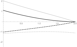
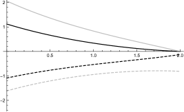
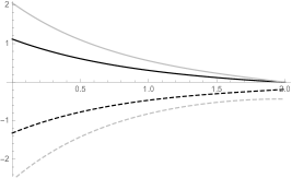
Figure 3: Equilibrium strategies $X^{*}_{i}(t)$ (solid) and trading rates $\dot{X}^{*}_{i}(t)$ (dashed) for agents $i=1$ (black) and $i=2$ (grey) as functions of $t\in[0,T]$ for $\alpha\sigma^{2}=0$ (left), $\alpha\sigma^{2}=0.8$ (center), and $\alpha\sigma^{2}=3$ (right); the remaining parameters are as in Figure 1. When $\alpha\sigma^{2}$ is increased from 0 to 0.8, agent 2 receives a relatively high increase in volatility risk and therefore speeds up liquidation throughout the first half of $[0,T]$, while slowing down in the second half. The volatility risk of agent 1 also increases, but it does so less than for agent 2 and leads only to a small initial increase of the liquidation speed $-\dot{X}_{1}^{*}(t)$. On the other hand, the increased price pressure from the temporary impact of agent 2 results in unfavorable asset prices for agent 1 in the first half of $[0,T]$, and this latter effect can outweigh the increased volatility risk to some extend. Therefore, it is beneficial for agent 1 to delay selling in the central part of the time interval $[0,T]$ and to compensate by accelerating the strategy toward the end. This effect leads to the increase of the intermediate asset position $X_{1}^{*}(1)$ as observed in Figure 1. When $\alpha\sigma^{2}$ increases even further, the increase in volatility risk becomes dominant, and so $X_{1}^{*}(1)$ starts to decrease again.

Figure 4: $X^{*}_{1}(1)$ as a function of $\lambda$ for $x_{1}=0.2$, $x_{2}=4$, $T=2$, $\alpha\sigma^{2}=1$, and $\gamma=0.3$.

Figure 5: $X^{*}_{1}(1)$ as a function of $\gamma$ for $x_{1}=0.86$, $x_{2}=0.28$, $T=2$, $\alpha\sigma^{2}=1$, and $\lambda=1$.

3 Nash equilibrium with infinite time horizon

Now, we consider mean-variance optimization and CARA utility maximization for an infinite time horizon $[0,\infty)$. Financially, this problem corresponds to a situation in which none of the agents faces a material time constraint. To simplify the discussion, we assume from the beginning that the drift $b(\cdot)$ vanishes identically. Then, the unaffected price process is given by $S^{0}(t)=S_{0}+\sigma W(t)$ for $t\geq 0$. Here, we need to assume that $\sigma\neq 0$. If only one agent is active, we are in the situation of Schied and Schöneborn (2009), where the problem of maximizing the expected utility of revenues is discussed for an infinite time horizon. As discussed there, a strategy $(X(t))_{t\geq 0}$ should satisfy the following conditions of admissibility so that the utility-maximization problem is well-defined for a single agent:
$\bullet$ $X$ is adapted to the filtration $({\mathscr{F}}_{t})_{t\geq 0}$;
$\bullet$ $X$ is absolutely continuous in the sense that $X(t)=X(0)+\int_{0}^{t}\dot{X}(s)\,ds$ for some progressively measurable process $(\dot{X}(t))_{t\geq 0}$ for which

$$\int_{0}^{\infty}(\dot{X}(t))^{2}\,dt<\infty\qquad\text{${\mathbb{P}}$-a.s.;}$$ (20)

$\bullet$ $X$ is bounded and satisfies

$${\mathbb{E}}\Big{[}\,\int_{0}^{\infty}X(t)^{2}\,dt\,\Big{]}<\infty\qquad\text{and}\qquad\lim_{t\uparrow\infty}(X(t))^{2}t\log\log t=0\text{ ${\mathbb{P}}$-a.s.}$$ (21)

The class of all strategies that are admissible in this sense and satisfy $X(0)=x$ for given $x\in\mathbb{R}$ will be denoted by ${\mathscr{X}}(x,\infty)$. As before, we denote by ${\mathscr{X}}_{\text{det}}(x,\infty)$ the subclass of all deterministic strategies in ${\mathscr{X}}(x,\infty)$. When the admissible strategy $X$ is used, the affected price process is

$$S^{X}(t)=S^{0}(t)+\gamma(X(t)-X(0))+\lambda\dot{X}(t).$$

It is shown in Schied and Schöneborn (2009, Section 3.1) that the total revenues of $X\in{\mathscr{X}}(x,\infty)$ are ${\mathbb{P}}$-a.s. well-defined as the limit

$$\mathscr{R}(X):=-\lim_{T\uparrow\infty}\int_{0}^{T}\dot{X}(t)S^{X}(t)\,dt=xS_{0}-\frac{\gamma}{2}x^{2}+\sigma\int_{0}^{\infty}X(t)\,dW(t)-\lambda\int_{0}^{\infty}(\dot{X}(t))^{2}\,dt$$

(see also Lemma 4.5 below). Moreover, for $\alpha>0$ and $u_{\alpha}$ as in (5), the unique strategy that maximizes the expected utility ${\mathbb{E}}[\,u_{\alpha}(\mathscr{R}(X))\,]$ over $X\in{\mathscr{X}}(x,\infty)$ is given by

$$X^{*}_{0}(t)=x\exp\Big{(}-t\sqrt{\frac{\alpha\sigma^{2}}{2\lambda}}\Big{)},\qquad t\geq 0;$$

see Corollary 4.4 in Schied and Schöneborn (2009). As $\mathscr{R}(X)$ is a Gaussian random variable for $X\in{\mathscr{X}}_{\text{det}}(x,\infty)$, one sees that

$${\mathbb{E}}[\,u_{\alpha}(\mathscr{R}(X))\,]=\frac{1}{\alpha}\Big{(}1-e^{-\alpha{\mathbb{E}}[\,\mathscr{R}(X)\,]+\frac{\alpha^{2}}{2}\text{var\,}(\mathscr{R}(X))}\Big{)},\qquad X\in{\mathscr{X}}_{\text{det}}(x,\infty),$$

and so $X^{*}_{0}$ also maximizes the mean-variance functional ${\mathbb{E}}[\,\mathscr{R}(X)\,]-\frac{\alpha}{2}\text{var\,}(\mathscr{R}(X))$ over $X\in{\mathscr{X}}_{\text{det}}(x,\infty)$.

When $n$ investors apply admissible strategies $X_{1},X_{2},\dots,X_{n}$, the affected price $S^{X_{1},\dots,X_{n}}(t)$ is again given by (6), as in the case of a finite time horizon. It will follow from Lemma 4.5 below that the admissibility of $X_{1},X_{2},\dots,X_{n}$ guarantees that the following limit exists ${\mathbb{P}}$-a.s.:

$$\mathscr{R}(X_{i}|\bm{X}_{-i}):=-\lim_{T\uparrow\infty}\int_{0}^{T}\dot{X}_{i}(t)S^{X_{1},\dots,X_{n}}(t)\,dt.$$

The Nash equilibria for mean-variance optimization and CARA utility maximization can now be defined by taking $T=\infty$ in Definition 2.1. Here is our result on the existence and uniqueness of Nash equilibria.

Theorem 3.1.

Suppose that one of the following two conditions holds:

1. $n\in\mathbb{N}$ is arbitrary and $\alpha_{1}=\cdots=\alpha_{n}=\alpha>0$;

2. $n=2$ and $\alpha_{1}$ and $\alpha_{2}$ are distinct and strictly positive.

Then, for all $x_{1},\dots,x_{n}\in\mathbb{R}$, there exists a unique Nash equilibrium $(X^{*}_{1},\dots,X^{*}_{n})$ for mean-variance optimization with infinite time horizon. Moreover, $(X^{*}_{1},\dots,X^{*}_{n})$ is also a Nash equilibrium for CARA utility maximization with infinite time horizon.

In case (a), the optimal strategies are given by

$$X^{*}_{i}(t)=(x_{i}-\overline{x}_{n})e^{\theta_{-}t}+\overline{x}_{n}e^{\rho_{-}t},$$ (22)

where again $\overline{x}_{n}=\frac{1}{n}\sum_{j=1}^{n}x_{j}$ and $\rho_{-}$ and $\theta_{-}$ are as in (12).

In case (b), the fourth-order equation

$$\tau^{4}-\frac{2\gamma}{3\lambda}\tau^{3}-\frac{\gamma^{2}+2\lambda\sigma^{2}(\alpha_{1}+\alpha_{2})}{3\lambda^{2}}\tau^{2}+\frac{\sigma^{4}\alpha_{1}\alpha_{2}}{3\lambda^{2}}=0$$

has precisely two distinct roots, $\tau_{1}$, $\tau_{2}$, in $(-\infty,0)$, and the equilibrium strategies $X^{*}_{1}(t)$ and $X^{*}_{2}(t)$ are linear combinations of the exponential functions $e^{\tau_{1}t}$ and $e^{\tau_{2}t}$.

On the one hand, the structure of the equilibrium strategies for an infinite time horizon appears to be simpler than for the finite-time situation. On the other hand, the assumptions of Theorem 3.1 are more restrictive than those of Theorem 2.2. More restrictive assumptions are needed, because all solutions $X_{1}(t),\dots,X_{n}(t)$ of the system (7) are linear combinations of exponential functions and thus can only take the limits $\pm\infty$ and $0$ for $t\uparrow\infty$. We must single out those with limit $0$. To this end, we cannot apply standard results on the existence of solutions for boundary value problems on noncompact intervals such as those in Cecchi et al. (1980), where it is required that the possible boundary values at $t=\infty$ include the full space $\mathbb{R}^{n}$. Instead, we show here that the eigenspaces associated with the negative eigenvalues of a certain nonsymmetric matrix $M$ are sufficiently rich. For $n>2$, we are only able to understand these eigenspaces when $\alpha_{1}=\cdots=\alpha_{n}$.

Remark 3.2.

In the situation of part (a) of Theorem 3.1, consider the corresponding Nash equilibrium $X_{1}^{(T)},\dots,X_{n}^{(T)}$ for the finite time interval $[0,T]$ as constructed in Theorem 2.5. Then, we conclude from (13) and (14) that

$$\lim_{T\uparrow\infty}X_{i}^{(T)}(t)=X_{i}^{*}(t),\qquad\text{for $i=1,\dots,n$ and $t\geq 0$,}$$

where $X_{i}^{*}$ is as in (22).

Let us finally discuss some qualitative properties of the Nash equilibrium in part (a) of Theorem 3.1. Carlin et al. (2007) and Schöneborn and Schied (2009) study, among other things, whether the liquidation of a large block of shares by agent 1 leads either to predatory trading or liquidity provision by the other agents if these all have zero initial capital (i.e., $x_{i}=0$ for $i\neq 1$). Here, predatory trading refers to a strategy during which the asset is shortened at the initial high price and then bought back later when the sell strategy of agent 1 has depreciated the asset price. This strategy is “predatory” in the sense that the revenues it generates for agent $i$ are made at the expense of agent 1. Liquidity provision refers to exactly the opposite strategy: agent $i$ acquires a long position by first buying and later re-selling some of the shares agent 1 is liquidating. It can hence be seen as a cooperative behavior on behalf of agent $i$. Both Carlin et al. (2007) and Schöneborn and Schied (2009) consider risk-neutral agents who need to close their positions in finite time. In Carlin et al. (2007), all agents face the same time constraint. In this case, liquidity provision can only be observed if cooperation is enforced by repeating the game. Schöneborn and Schied (2009) admit a longer time horizon for agents $i=2,\dots,n$ than for agent 1 and find that this relaxation can lead to liquidity provision for certain parameter values without having to repeat the game. Our corresponding result is Corollary 3.3 below. It states that, on an infinite time horizon, both predatory trading and liquidity provision can occur, depending on the parameters of the model; see also Figure 6 for an illustration. Together with Remark 3.2, Corollary 3.3 implies that liquidity provision can also occur if all agents share the same time horizon $T$, provided that $T$ is sufficiently large. This fact that is markedly different from the risk-neutral case $\alpha=0$ considered in Carlin et al. (2007).

Corollary 3.3.

In the situation of part (a) of Theorem 3.1, suppose that $\sum_{i=1}^{n}x_{i}>0$. Then an agent with $x_{i}=0$ engages in liquidity provision in the sense that $X^{*}_{i}(t)>0$ for all $t>0$, if and only if $\alpha\sigma^{2}\lambda>2\gamma^{2}$. When $\alpha\sigma^{2}\lambda<2\gamma^{2}$ this agent engages in predatory trading, and for $\alpha\sigma^{2}\lambda=2\gamma^{2}$ the agent does not trade at all.

Finally, we briefly discuss the behavior of equilibrium strategies as a function of the number $n$ of agents active in the market. Lebedeva et al. (2012) discuss the following two hypotheses and analyze their validity for a large data set of block executions by large insiders:
Hypothesis 1: “Trade duration decreases if several insiders compete for exploiting the same long-lived information.”
Hypothesis 2: “Trade duration increases if several insiders trade simultaneously in the same direction for liquidity reasons.”
In the situation of part (a) of our Theorem 3.1, the effective trade duration can be both increasing or decreasing in $n$, or even lack monotonicity entirely; see Figure 7. Here, the effective trade duration is defined as the time until a certain high percentage of the initial inventory has been liquidated. So both hypotheses from Lebedeva et al. (2012) are compatible with risk-averse agents in an Almgren–Chriss setting.

Figure 6: Strategies $X^{*}_{i}(t)$ for $\lambda=0.15$ (left) and $\lambda=0.16$ (right) for various choices of $n$ and for $x_{i}=0$, $\sum_{j=1}^{n}x_{j}=1$, $\gamma=0.16$, and $\alpha\sigma^{2}=0.33$.

Figure 7: Effective liquidation time of $X^{*}_{1}$, defined as the time until 99% of the initial inventory $x_{1}$ have been liquidated, plotted as a function of $n\in\{1,\dots,40\}$. In the left-hand panel, we we see that monotonicity in $n$ can be reversed by a very small change in $\gamma$; we took $\gamma=0.155$ (circles) and $\gamma=0.16$ (bullets) with $x_{1}=1$, $\sum_{i=1}^{n}x_{i}=3.5$, $\lambda=0.15$, and $\alpha\sigma^{2}=0.33$. In the right-hand panel, we observe that the effective liquidation time need not be monotone in $n$; here we chose $x_{1}=5$, $\sum_{i=1}^{n}x_{i}=10$, $\lambda=2$, $\gamma=0.1$, and $\alpha\sigma^{2}=0.33$.

4 Proofs

4.1 Proofs for a finite time horizon

Let admissible strategies $X_{i}\in{\mathscr{X}}(x_{i},T)$ be given and write $\bm{X}_{-i}:=\{X_{1},\dots,X_{i-1},X_{i+1},\dots,X_{n}\}$ for $i=1,\dots,n$. For $Y\in{\mathscr{X}}(y,T)$, we note first that, after integrating by parts,

$$\mathscr{R}(Y|\bm{X}_{-i}) =yS_{0}-\frac{\gamma}{2}y^{2}+\int_{0}^{T}Y(t)\Big{(}b(t)+\gamma\sum_{j\neq i}\dot{X}_{j}(t)\Big{)}\,dt$$

$$\qquad-\lambda\sum_{j\neq i}^{n}\int_{0}^{T}\dot{Y}(t)\dot{X}_{j}(t)\,dt-\lambda\int_{0}^{T}\dot{Y}(t)^{2}\,dt+\sigma\int_{0}^{T}Y(t)\,dW(t).$$

When all $X_{i}$ and $Y$ are deterministic, it follows that

$${\mathbb{E}}[\,\mathscr{R}(Y|\bm{X}_{-i})\,]-\frac{\alpha_{i}}{2}\,\text{var\,}(\mathscr{R}(Y|\bm{X}_{-i}))=c+\int_{0}^{T}\mathscr{L}^{i}(t,Y(t),\dot{Y}(t)|\bm{X}_{-i})\,dt,$$ (23)

where $c=yS_{0}-\frac{\gamma}{2}y^{2}$ and the Lagrangian $\mathscr{L}^{i}$ is given by

$$\mathscr{L}^{i}(t,q,p|\bm{X}_{-i})=q\Big{(}b(t)+\gamma\sum_{j\neq i}\dot{X}_{j}(t)\Big{)}-\frac{{\alpha_{i}}\sigma^{2}}{2}q^{2}-\lambda p\Big{(}\sum_{j\neq i}\dot{X}_{j}(t)+p\Big{)}.$$ (24)

Lemma 4.1.

In the context of Theorem 2.2, there exists at most one Nash equilibrium for mean-variance optimization.

Proof.

We assume by way of contradiction that $X^{0}_{1},\dots,X^{0}_{n}$ and $X^{1}_{0},\dots,X^{1}_{n}$ are two distinct Nash equilibria with $X^{k}_{i}\in{\mathscr{X}}(x_{i},T)$ for $i=1,\dots,n$ and $k=0,1$. For $\beta\in[0,1]$, let $X^{\beta}_{i}:=\beta X^{1}_{i}+(1-\beta)X^{0}_{i}$ and define

$$f(\beta):=\sum_{i=1}^{n}\int_{0}^{T}\Big{(}\mathscr{L}^{i}(t,X_{i}^{\beta}(t),\dot{X}_{i}^{\beta}(t)|{\bm{X}}^{0}_{-i})+\mathscr{L}^{i}(t,X_{i}^{1-\beta}(t),\dot{X}_{i}^{1-\beta}(t)|{\bm{X}}^{1}_{-i})\Big{)}\,dt.$$

By assumption, the strategy $X_{i}^{k}$ maximizes the functional $Y\mapsto\int_{0}^{T}\mathscr{L}^{i}(t,Y(t),\dot{Y}(t)|{\bm{X}}^{k}_{-i})\,dt$ within the class ${\mathscr{X}}_{\text{det}}(x_{i},T)$ for $k=0,1$. We therefore must have $f(\beta)\leq f(0)$ for $\beta>0$, which implies that

$$\frac{d}{d\beta}\Big{|}_{\beta=0+}f(\beta)\leq 0.$$ (25)

On the other hand, by interchanging differentiation and integration, which is permitted due to our assumptions on admissible strategies and due to the linear-quadratic form of the Lagrangian, a short computation shows that

$$\frac{d}{d\beta}\Big{|}_{\beta=0+}f(\beta)$$

$$=\sum_{i=1}^{n}\int_{0}^{T}\bigg{[}\gamma(X^{1}_{i}(t)-X^{0}_{i}(t))\sum_{j=1}^{n}(\dot{X}_{j}^{0}(t)-\dot{X}_{j}^{1}(t))-\gamma(X^{1}_{i}(t)-X^{0}_{i}(t))(\dot{X}_{i}^{0}(t)-\dot{X}^{1}_{i}(t))$$

$$\quad+{\alpha_{i}}\sigma^{2}(X^{1}_{i}(t)-X^{0}_{i}(t))^{2}+\lambda(\dot{X}^{1}_{i}(t)-\dot{X}^{0}_{i}(t))\sum_{j=1}^{n}(\dot{X}^{1}_{j}(t)-\dot{X}_{j}^{0}(t))+\lambda(\dot{X}^{0}_{i}(t)-\dot{X}^{1}_{i}(t))^{2}\bigg{]}\,dt.$$

We note next that

$$\int_{0}^{T}(X^{1}_{i}(t)-X^{0}_{i}(t))(\dot{X}^{0}_{i}(t)-\dot{X}^{1}_{i}(t))\,dt=\frac{1}{2}(X^{1}_{i}(T)-X^{0}_{i}(T))^{2}-\frac{1}{2}(X^{1}_{i}(0)-X^{0}_{i}(0))^{2}=0.$$

Moreover, by the same argument,

$$\int_{0}^{T}(X^{1}_{i}(t)-X^{0}_{i}(t))(\dot{X}^{0}_{j}(t)-\dot{X}^{1}_{j}(t))\,dt=-\int_{0}^{T}(X^{1}_{j}(t)-X^{0}_{j}(t))(\dot{X}^{0}_{i}(t)-\dot{X}^{1}_{i}(t))\,dt,$$

and hence

$$\sum_{i=1}^{n}\sum_{j=1}^{n}\int_{0}^{T}(X^{1}_{i}(t)-X^{0}_{i}(t))(\dot{X}^{0}_{j}(t)-\dot{X}^{1}_{j}(t))\,dt=0.$$

It follows that

$${\frac{d}{d\beta}\Big{|}_{\beta=0+}f(\beta)}=\int_{0}^{T}\bigg{[}{\alpha_{i}}\sigma^{2}\sum_{i=1}^{n}(X^{1}_{i}(t)-X^{0}_{i}(t))^{2}+\lambda\sum_{i=1}^{n}(\dot{X}^{0}_{i}(t)-\dot{X}^{1}_{i}(t))^{2}+\lambda\Big{(}\sum_{i=1}^{n}(\dot{X}^{0}_{i}(t)-\dot{X}^{1}_{i}(t))\Big{)}^{2}\bigg{]}\,dt,$$

which is strictly positive because the two Nash equilibria $X^{0}_{1},\dots,X^{0}_{n}$ and $X^{1}_{0},\dots,X^{1}_{n}$ are distinct. But strict positivity contradicts (25). ∎

Lemma 4.2.

For $i=1,\dots,n$ there exists at most one maximizer in ${\mathscr{X}}_{\text{det}}(y,T)$ of the functional $Y\mapsto\int_{0}^{T}\mathscr{L}^{i}(t,Y(t),\dot{Y}(t)|\bm{X}_{-i})\,dt$. If, moreover, $X_{1},\dots,X_{n}\in C^{2}[0,T]$, then there exists a unique maximizer $Y^{*}\in{\mathscr{X}}_{\text{det}}(y,T)\cap C^{2}[0,T]$, which is given as the unique solution of the two-point boundary value problem

$$\left\{\begin{array}[]{l}{\alpha_{i}}\sigma^{2}Y(t)-2\lambda\ddot{Y}(t)=b(t)+\gamma\sum_{j\neq i}\dot{X}_{j}(t)+\lambda\sum_{j\neq i}\ddot{X}_{j}(t),\\ Y(0)=y,\ Y(T)=0.\end{array}\right.$$

Proof.

It follows from the strict concavity of the Lagrangian $\mathscr{L}^{i}$ and the convexity of the set ${\mathscr{X}}_{\text{det}}(y,T)$ that there can be at most one maximizer in ${\mathscr{X}}_{\text{det}}(y,T)$.

Now, we show the existence of a maximizer under the additional assumption $X_{1},\dots,X_{n}\in C^{2}[0,T]$. Under this assumption, we may formulate the Euler–Lagrange equation $\mathscr{L}^{i}_{q}(t,Y(t),\dot{Y}(t)|\bm{X}_{-i})=\frac{d}{dt}\mathscr{L}^{i}_{p}(t,Y(t),\dot{Y}(t)|\bm{X}_{-i})$, which for our specific Lagrangian becomes:

$${\alpha_{i}}\sigma^{2}Y(t)-2\lambda\ddot{Y}(t)=b(t)+\gamma\sum_{j\neq i}\dot{X}_{j}(t)+\lambda\sum_{j\neq i}\ddot{X}_{j}(t).$$ (26)

Denoting the right-hand side of (26) by $u(t)$, the general solution of this second-order ODE is of the form

$$Y(t)=c_{1}e^{-\kappa_{i}t}+c_{2}e^{\kappa_{i}t}-\frac{1}{4\lambda\kappa_{i}}\int_{0}^{t}e^{\kappa_{i}(t-s)}u(s)\,ds+\frac{1}{4\lambda\kappa_{i}}\int_{0}^{t}e^{-\kappa_{i}(t-s)}u(s)\,ds,$$

where $c_{1}$ and $c_{2}$ are constants and $\kappa_{i}=\sqrt{{\alpha_{i}\sigma^{2}}/{2\lambda}}$. It is clear that the two constants $c_{1}$ and $c_{2}$ can be uniquely determined by imposing the boundary conditions $Y(0)=y$ and $Y(T)=0$. From now on, let $Y^{*}\in{\mathscr{X}}_{\text{det}}(y,T)\cap C^{2}[0,T]$ denote the corresponding solution. We will now verify that $Y^{*}$ is indeed a maximizer of our problem. To this end, let $Y\in{\mathscr{X}}_{\text{det}}(y,T)$ be arbitrary. Using first the concavity of $(q,p)\mapsto\mathscr{L}^{i}(t,q,p|\bm{X}_{-i})$ and then the fact that $Y^{*}$ solves the Euler–Lagrange equation, we get

$$\mathscr{L}^{i}(t,Y^{*}(t),\dot{Y}^{*}(t)|\bm{X}_{-i}))-\mathscr{L}^{i}(t,Y(t),\dot{Y}(t)|\bm{X}_{-i})$$

$$\geq\mathscr{L}^{i}_{q}(t,Y^{*}(t),\dot{Y}^{*}(t)|\bm{X}_{-i}))(Y^{*}(t)-Y(t))+\mathscr{L}^{i}_{p}(t,Y^{*}(t),\dot{Y}^{*}(t)|\bm{X}_{-i}))(\dot{Y}^{*}(t)-\dot{Y}(t))$$

$$=\Big{(}\frac{d}{dt}\mathscr{L}^{i}_{p}(t,Y^{*}(t),\dot{Y}^{*}(t)|\bm{X}_{-i})\Big{)}(Y^{*}(t)-Y(t))+\mathscr{L}^{i}_{p}(t,Y^{*}(t),\dot{Y}^{*}(t)|\bm{X}_{-i}))(\dot{Y}^{*}(t)-\dot{Y}(t))$$

$$=\frac{d}{dt}\Big{(}\mathscr{L}^{i}_{p}(t,Y^{*}(t),\dot{Y}^{*}(t)|\bm{X}_{-i})(Y^{*}(t)-Y(t))\Big{)}.$$

Therefore,

$$\int_{0}^{T}\mathscr{L}^{i}(t,Y^{*}(t),\dot{Y}^{*}(t)|\bm{X}_{-i})\,dt-\int_{0}^{T}\mathscr{L}^{i}(t,Y(t),\dot{Y}(t)|\bm{X}_{-i})\,dt$$

$$\geq\int_{0}^{T}\frac{d}{dt}\Big{(}\mathscr{L}^{i}_{p}(t,Y^{*}(t),\dot{Y}^{*}(t)|\bm{X}_{-i})(Y^{*}(t)-Y(t))\Big{)}\,dt=0,$$

where in the final step we have used that $Y^{*}(0)=Y(0)$ and $Y^{*}(T)=Y(T)$. This proves the lemma. ∎

Proof of Theorem 2.2.

According to Lemma 4.1, there exists at most one Nash equilibrium. We will now show that there exists a Nash equilibrium $X^{*}_{1},\dots,X^{*}_{n}$ such that each strategy $X^{*}_{i}$ belongs to ${\mathscr{X}}_{\text{det}}(x_{i},T)\cap C^{2}[0,T]$. By Lemma 4.2, each strategy $X^{*}_{i}$ must then be a solution of the second-order differential equation

$${\alpha_{i}}\sigma^{2}X_{i}(t)-2\lambda\ddot{X}_{i}(t)=b(t)+\gamma\sum_{j\neq i}\dot{X}^{*}_{j}(t)+\lambda\sum_{j\neq i}\ddot{X}^{*}_{j}(t),$$ (27)

with boundary conditions

$$X_{i}(0)=x_{i} X_{i}(T)=0$$ and . (28)

We can clearly combine the $n$ differential equations (27) into a system of $n$ coupled second-order linear ordinary differential equations for the vector $\bm{X}^{*}:=(X^{*}_{1},\dots,X^{*}_{n})^{\top}$. It follows again from Lemma 4.2 that every $C^{2}$-solution of the system (27), (28) is a Nash equilibrium. Therefore the assertion of the theorem will follow if we can show the existence of a $C^{2}$-solution to the $n$-dimensional two-point boundary value problem (27), (28).

By introducing the auxiliary function $\bm{Y}(t)$ for the derivative $\dot{\bm{X}}(t)$, by letting $\bm{b}(t)$ be the vector with all components equal to $b(t)$, and by defining the $n\times n$ matrices $A:=\sigma^{2}\text{diag}(\alpha_{1},\dots,\alpha_{n})$, the identity matrix $I=\text{diag}(1,\dots,1)$, and the matrix $J$ with all entries equal to one, the system (27) can be re-written as follows:

$$\begin{pmatrix}A&-\gamma(J-I)\\ 0&I\end{pmatrix}\begin{pmatrix}\bm{X}(t)\\ \bm{Y}(t)\end{pmatrix}-\begin{pmatrix}0&\lambda(J+I)\\ I&0\end{pmatrix}\begin{pmatrix}\dot{\bm{X}}(t)\\ \dot{\bm{Y}}(t)\end{pmatrix}=\begin{pmatrix}\bm{b}(t)\\ \bm{0}\end{pmatrix}.$$ (29)

Clearly, $\bm{X}$ is a $C^{2}$-solution of (27) if and only if ${\bm{X}\choose\dot{\bm{X}}}$ is a $C^{1}$-solution of (29). In particular, every $C^{1}$-solution of (29) with boundary conditions (28) yields a Nash equilibrium.

Now consider the homogeneous system (29), (28) with $\bm{b}(t)=0$ and initial values $x_{1}=\cdots=x_{n}=0$. The corresponding boundary condition can be written as

$$(\bm{X}(0),\bm{Y}(0),\bm{X}(T),\bm{Y}(T))^{\top}\in V,$$ (30)

where $V\subset\mathbb{R}^{4n}$ is the $2n$-dimensional linear space

$$V=\big{\{}(\bm{x}_{0},\bm{y}_{0},\bm{x}_{1},\bm{y}_{1})^{\top}\in\mathbb{R}^{4n}\,|\,\bm{x}_{0}=\bm{x}_{1}=\bm{0}\big{\}}.$$

It is clear that ${\bm{X}\choose{\bm{Y}}}={\bm{0}\choose\bm{0}}$ is a solution. In fact, this trivial solution is the only solution as every solution must be a Nash equilibrium, and Nash equilibria are unique by Lemma 4.1. It therefore follows from the general theory of linear boundary value problems for systems of ordinary differential equations that the two-point boundary value problem (29), (30) has a unique $C^{1}$-solution for every continuous $\bm{b}:[0,T]\to\mathbb{R}^{n}$ (and in fact for every continuous $\mathbb{R}^{2n}$-valued function substituting ${\bm{b}(t)\choose\bm{0}}$ on the right-hand side of (29)); see Kurzweil (1986, (9.22), p. 189). Using this fact, we let ${\bm{X}^{0}\choose{\bm{Y}}^{0}}$ be the solution of (29), (30) when $\bm{b}(t)$ in (29) is replaced by $\bm{b}^{0}(t)=(b_{1}^{0}(t),\dots,b^{0}_{n}(t))$ for

$$b^{0}_{i}(t)=b(t)+\frac{T-t}{T}\alpha_{i}\sigma^{2}x_{i}+\frac{\gamma}{T}\sum_{j\neq i}x_{j}.$$

One then checks that

$$X_{i}^{*}(t):=X^{0}_{i}(t)+\frac{T-t}{T}x_{i},\qquad i=1,\dots,n,$$

solves (27), (28) and is thus the desired Nash equilibrium. ∎

Remark 4.3.

For $A:=\sigma^{2}\text{diag}(\alpha_{1},\dots,\alpha_{n})$, the identity matrix $I$, and the matrix $J$ with all entries equal to one, let

$$M:=\begin{pmatrix}0&\lambda(J+I)\\ I&0\end{pmatrix}^{-1}\begin{pmatrix}A&-\gamma(J-I)\\ 0&I\end{pmatrix}.$$

and

$$\bm{f}(t):=-\begin{pmatrix}0&\lambda(J+I)\\ I&0\end{pmatrix}^{-1}\begin{pmatrix}\bm{b}(t)\\ \bm{0}\end{pmatrix}.$$

With this notation and $\bm{Z}(t):=(\bm{X}(t),\bm{Y}(t))^{\top}$, the system (29) can now be written as

$$\dot{\bm{Z}}(t)=M\bm{Z}(t)+\bm{f}(t).$$ (31)

Note that $J^{2}=nJ$ and that hence $(J+I)(I-\frac{1}{n+1}J)=I=(I-\frac{1}{n+1}J)(J+I)$. It follows that

$$\begin{pmatrix}0&\lambda(J+I)\\ I&0\end{pmatrix}^{-1}=\begin{pmatrix}0&I\\ \frac{1}{\lambda}(I-\frac{1}{n+1}J)&0\end{pmatrix},$$

and hence that

$$M=\begin{pmatrix}0&I\\ \frac{1}{\lambda}(A-\frac{1}{n+1}JA)&\frac{\gamma}{\lambda}(I-\frac{2}{n+1}J)\end{pmatrix}.$$ (32)

Proof of Corollary 2.3.

Let $X^{*}_{1},\dots,X^{*}_{n}$ be the unique Nash equilibrium for mean-variance optimization as constructed in Theorem 2.2. When ${\bm{X}}^{*}_{-i}=\{X^{*}_{1},\dots,X^{*}_{i-1},X^{*}_{i+1},\dots,X^{*}_{n}\}$ is fixed, the $i^{\text{th}}$ agent perceives

$$S^{{\bm{X}}^{*}_{-i}}(t):=S^{0}(t)+\gamma\sum_{j\neq i}(X_{j}(t)-X_{j}(0))+\lambda\sum_{j\neq i}\dot{X}_{j}(t),\qquad t\in[0,T],$$

as “unaffected” price process. It is of the form

$$S^{{\bm{X}}^{*}_{-i}}(t)=S_{0}+\sigma W(t)+\int_{0}^{t}b^{i}(s)\,ds$$

for a deterministic and continuous function $b^{i}:[0,T]\to\mathbb{R}$. As the process $S^{{\bm{X}}^{*}_{-i}}$ has independent increments and $S^{{\bm{X}}^{*}_{-i}}_{T}$ has all exponential moments, i.e., ${\mathbb{E}}\big{[}\,e^{\beta S^{{\bm{X}}^{*}_{-i}}_{t}}\,\big{]}<\infty$ for all $\beta\in\mathbb{R}$ and $t\geq 0$, it follows as in Schied et al. (2010, Theorem 2.1) that for $\alpha_{i}>0$

$$\sup_{X\in{\mathscr{X}}(x_{i},T)}{\mathbb{E}}[\,u_{\alpha_{i}}(\mathscr{R}(X|\bm{X}_{-i}))\,]=\sup_{X\in{\mathscr{X}}_{\text{det}}(x_{i},T)}{\mathbb{E}}[\,u_{\alpha_{i}}(\mathscr{R}(X|\bm{X}_{-i}))\,].$$

But for $\alpha_{i}>0$ and $X\in{\mathscr{X}}_{\text{det}}(x_{i},T)$ we have

$${\mathbb{E}}[\,u_{\alpha_{i}}(\mathscr{R}(X|\bm{X}_{-i}))\,]=\frac{1}{\alpha_{i}}\Big{(}1-e^{-\alpha_{i}{\mathbb{E}}[\,\mathscr{R}(X|\bm{X}_{-i})\,]+\frac{\alpha_{i}^{2}}{2}\,\text{var\,}(\mathscr{R}(X|\bm{X}_{-i})}\Big{)},$$

which shows that CARA utility maximization is equivalent to the maximization of the corresponding mean-variance functional. The corresponding result for $\alpha_{i}=0$ is obvious. ∎

Proof of Corollary 2.4.

Letting $\Sigma(t):=\sum_{j=1}^{n}X_{j}(t)$ and re-writing (7) yields

$${\alpha}\sigma^{2}X_{i}(t)+\gamma\dot{X}_{i}(t)-\lambda\ddot{X}_{i}(t)=b(t)+\gamma\dot{\Sigma}(t)+\lambda\ddot{\Sigma}(t)$$

and hence (10). Summing over $i$ then implies (9). ∎

Now we prepare for the proof of Theorem 2.5.

Lemma 4.4.

For $\alpha_{1}=\cdots=\alpha_{n}=\alpha>0$, the matrix $M$ from (32) has four real eigenvalues $\theta_{+},\theta_{-},\rho_{+},\rho_{-}$ given by (12). Moreover, with $\bm{1}\in\mathbb{R}^{n}$ denoting the vector with all entries equal to $1$, the corresponding eigenspaces are given by

$$E(\rho_{\pm})=\text{\rm span}{\bm{1}\choose\rho_{\pm}\bm{1}}\qquad\text{and}\qquad E(\theta_{\pm})=\bigg{\{}{\bm{v}\choose\theta_{\pm}\bm{v}}\,\Big{|}\,\bm{v}\in\mathbb{R}^{n},\ \bm{v}\perp\bm{1}\bigg{\}}.$$

Proof.

Let us write an arbitrary vector in $\mathbb{R}^{2n}$ as ${\bm{v}_{1}\choose\bm{v}_{2}}$ for $\bm{v}_{1},\bm{v}_{2}\in\mathbb{R}^{n}$. By applying $M$ to ${\bm{v}_{1}\choose\bm{v}_{2}}$ we see that we must have $\bm{v}_{2}=\tau\bm{v}_{1}$ for ${\bm{v}_{1}\choose\bm{v}_{2}}$ to be an eigenvector with eigenvalue $\tau$. So let us consider vectors in $\mathbb{R}^{2n}$ of the form ${\bm{v}\choose\tau\bm{v}}$ for $\bm{v}\in\mathbb{R}^{n}$ and $\tau\in\mathbb{R}$. The equation $M{\bm{v}\choose\tau\bm{v}}=\tau{\bm{v}\choose\tau\bm{v}}$ is equivalent to

$$\Big{(}\frac{\alpha\sigma^{2}}{\lambda}+\frac{\tau\gamma}{\lambda}\Big{)}\bm{v}-\frac{\alpha\sigma^{2}+2\tau\gamma}{{\lambda(n+1)}}J\bm{v}=\tau^{2}\bm{v}.$$ (33)

When $\bm{v}=\bm{1}$, then $J\bm{v}=n\bm{v}$ and (33) becomes the quadratic equation

$$\alpha\sigma^{2}+\gamma\tau-\frac{n(\alpha\sigma^{2}+2\gamma\tau)}{n+1}-\lambda\tau^{2}=0,$$

which is solved for $\tau=\rho_{+}$ and $\tau=\rho_{-}$. When $\bm{v}\perp\bm{1}$, then $J\bm{v}=0$ and (33) becomes the quadratic equation

$$\alpha\sigma^{2}+\gamma\tau-\lambda\tau^{2}=0,$$

which is solved for $\tau=\theta_{+}$ and $\tau=\theta_{-}$. As the eigenvectors found thus far span the entire space $\mathbb{R}^{2n}$, the proof is complete. ∎

Proof of Theorem 2.5..

It follows from Theorem 2.2 and its proof that $X^{*}_{1},\dots,X^{*}_{n}$ are obtained from the solutions of (31) for $\bm{f}(t)=\bm{0}$. The general solution of this system is of the form $\bm{Z}(t)=e^{tM}\bm{Z}(0)$. By Lemma 4.4, $M$ is diagonalizable and so every solution $\bm{Z}(t)$ must be a linear combination of exponential functions $e^{\tau t}$, where $\tau$ is an eigenvalue of $M$. Another application of Lemma 4.4 thus implies that each $X^{*}_{i}$ can be represented as in (13). One finally checks that for $c_{i}(\theta_{+}),c_{i}(\theta_{-}),c(\rho_{+}),c(\rho_{-})$ as in (14) the boundary conditions $X^{*}_{i}(0)=x_{i}$ and $X^{*}_{i}(T)=0$ are satisfied. That $\Sigma$ from (15) solves the two-point boundary problem (9) can be verified by a straightforward computation.∎

Proof of Corollary 2.6.

From (15) we have that $\Sigma(t)=X_{1}^{*}(t)+X_{2}^{*}(t)$ is given by (17). When letting $\Delta(t):=X^{*}_{1}(t)-X^{*}_{2}(t)$, we get from (10) that $\Delta$ solves the two-point boundary value problem

$$\alpha\sigma^{2}\Delta(t)+\gamma\dot{\Delta}(t)-\lambda\ddot{\Delta}(t)=0,\qquad\Delta(0)=x_{1}-x_{2},\ \Delta(T)=0.$$

This boundary value problem is solved by (18). ∎

4.2 Proofs for an infinite time horizon

Lemma 4.5.

For $X_{i}\in{\mathscr{X}}(x_{i},\infty)$ and $i=1,\dots,n$, the limit $\mathscr{R}(X_{i}|\bm{X}_{-i}):=-\lim_{T\uparrow\infty}\int_{0}^{T}\dot{X}_{i}(t)S^{X_{1},\dots,X_{n}}(t)\,dt$ exists, is finite, and is given by

$$\mathscr{R}(X_{i}|\bm{X}_{-i})=x_{i}S_{0}-\frac{\gamma}{2}x_{i}^{2}+\sigma\int_{0}^{\infty}\!\!X_{i}(t)\,dW(t)+\gamma\sum_{j\neq i}\int_{0}^{\infty}\!\!X_{i}(t)\dot{X}_{j}(t)\,dt-\lambda\sum_{j=1}^{n}\int_{0}^{\infty}\!\!\dot{X}_{i}(t)\dot{X}_{j}(t)\,dt.$$

Proof.

Integrating by parts yields

$$-\int_{0}^{T}\dot{X}_{i}(t)S^{X_{1},\dots,X_{n}}(t)\,dt$$

$$\qquad=(x_{i}-X_{i}(T))S_{0}-X(T)W(T)+\sigma\int_{0}^{T}X_{i}(t)\,dW(t)-\frac{\gamma}{2}(X_{i}(T)-X_{i}(0))^{2}$$

$$\qquad\qquad-\gamma\sum_{j\neq i}X_{i}(T)(X_{j}(T)-X_{j}(0))+\gamma\sum_{j\neq i}\int_{0}^{T}X_{i}(t)\dot{X}_{j}(t)\,dt-\lambda\sum_{j=1}^{n}\int_{0}^{T}\dot{X}_{i}(t)\dot{X}_{j}(t)\,dt.$$

The assertion now follows by using the law of the iterated logarithm for $W$, (20), (21), and the Cauchy–Schwarz inequality. ∎

Now let $X_{i}\in{\mathscr{X}}(x_{i},\infty)$, $i=1,\dots,n$, be given. As in (23), (24), we get that for $Y\in{\mathscr{X}}(y,\infty)$,

$${\mathbb{E}}[\,\mathscr{R}(Y|\bm{X}_{-i})\,]-\frac{\alpha_{i}}{2}\,\text{var\,}(\mathscr{R}(Y|\bm{X}_{-i}))=c+\int_{0}^{\infty}\mathscr{L}^{i}(t,Y(t),\dot{Y}(t)|\bm{X}_{-i})\,dt,$$

where $c=yS_{0}-\frac{\gamma}{2}y^{2}$ and the Lagrangian $\mathscr{L}^{i}$ is given by (24). Recall that we assume $\sigma^{2}>0$.

Lemma 4.6.

For $i=1,\dots,n$ and $\alpha_{i}>0$, the functional $Y\mapsto\int_{0}^{\infty}\mathscr{L}^{i}(t,Y(t),\dot{Y}(t)|\bm{X}_{-i})\,dt$ has at most one maximizer in ${\mathscr{X}}_{\text{det}}(y,\infty)$. If, moreover, $X_{1},\dots,X_{n}$ belong to $C^{2}[0,\infty)$ and are such that

$$\int_{0}^{\infty}\bigg{|}\gamma\sum_{j\neq i}\dot{X}_{j}(t)+\lambda\sum_{j\neq i}\ddot{X}_{j}(t)\bigg{|}\,dt<\infty,$$ (34)

then there exists a unique maximizer $Y^{*}\in{\mathscr{X}}_{\text{det}}(y,\infty)\cap C^{2}[0,\infty)$, which is given as the unique solution of the boundary value problem

$${\alpha_{i}}\sigma^{2}Y(t)-2\lambda\ddot{Y}(t)=\gamma\sum_{j\neq i}\dot{X}_{j}(t)+\lambda\sum_{j\neq i}\ddot{X}_{j}(t),\qquad Y(0)=y,\ \lim_{t\uparrow\infty}Y(t)=0.$$ (35)

Moreover, $Y$ satisfies $\int_{0}^{\infty}|\dot{Y}(t)|+|\ddot{Y}(t)|\,dt<\infty$.

Proof.

It follows from the strict concavity of the Lagrangian $\mathscr{L}^{i}$, the convexity of the set ${\mathscr{X}}_{\text{det}}(y,\infty)$, and the finiteness of the integral $\int_{0}^{\infty}\mathscr{L}^{i}(t,Y(t),\dot{Y}(t)|\bm{X}_{-i})\,dt$ that there can be at most one maximizer in ${\mathscr{X}}_{\text{det}}(y,\infty)$.

Now, we show the existence of a maximizer under the additional assumptions $X_{1},\dots,X_{n}\in C^{2}[0,\infty)$ and (34). As noted in the proof of Lemma 4.2, the general solution of the Euler–Lagrange equation (26) is given by

$$Y(t)=c_{1}e^{-\kappa_{i}t}+c_{2}e^{\kappa_{i}t}-\frac{1}{4\lambda\kappa_{i}}\int_{0}^{t}e^{\kappa_{i}(t-s)}u(s)\,ds+\frac{1}{4\lambda\kappa_{i}}\int_{0}^{t}e^{-\kappa_{i}(t-s)}u(s)\,ds,$$ (36)

where $u(t)=\gamma\sum_{j\neq i}\dot{X}_{j}(t)+\lambda\sum_{j\neq i}\ddot{X}_{j}(t)$, $c_{1}$ and $c_{2}$ are constants, and $\kappa_{i}=\sqrt{{\alpha_{i}\sigma^{2}}/{2\lambda}}>0$. One checks that (34) implies that $\int_{0}^{t}e^{-\kappa_{i}(t-s)}u(s)\,ds\to 0$ as $t\uparrow\infty$. Therefore, when letting

$$c_{2}:=\frac{1}{4\lambda\kappa_{i}}\int_{0}^{\infty}e^{-\kappa_{i}s}u(s)\,ds$$ (37)

and $c_{1}:=y-c_{2}$, one sees that the corresponding function $Y^{*}$ solves (35).

Next, by (35), (36), and (37), $Y^{*}(t)$, $\dot{Y}^{*}(t)$, and $\ddot{Y}^{*}(t)$ are linear combinations of the following functions:

$$u(t),\quad e^{-\kappa_{i}t},\quad\int_{0}^{t}e^{-\kappa_{i}(t-s)}u(s)\,ds,\quad\int_{t}^{\infty}e^{\kappa_{i}(t-s)}u(s)\,ds.$$

We have

$$\int_{0}^{T}\int_{0}^{t}e^{-\kappa_{i}(t-s)}|u(s)|\,ds\,dt=\frac{1}{\kappa_{i}}\int_{0}^{T}|u(s)|\,ds-\frac{1}{\kappa_{i}}\int_{0}^{T}e^{-\kappa_{i}(T-s)}|u(s)|\,ds$$

and

$$\int_{0}^{T}\int_{t}^{\infty}e^{\kappa_{i}(t-s)}|u(s)|\,ds\,dt=\frac{1}{\kappa_{i}}\int_{0}^{\infty}(e^{\kappa_{i}(s\wedge T-s)}-1)|u(s)|\,ds,$$

which by (34) both converge to finite limits for $T\uparrow\infty$. It thus follows that $\int_{0}^{\infty}|\dot{Y}^{*}(t)|+|\ddot{Y}^{*}(t)|\,dt<\infty$. In the same way, we get $\int_{0}^{\infty}|Y^{*}(t)|\,dt<\infty$. Adding the facts that $Y^{*}$ is continuous and tends to zero as $t\uparrow\infty$, we obtain $\int_{0}^{\infty}(Y^{*}(t))^{2}\,dt<\infty$ and in turn $Y^{*}\in{\mathscr{X}}_{\text{det}}(y,\infty)\cap C^{2}[0,\infty)$. The optimality of $Y^{*}$ follows as in the second part of the proof of Lemma 4.2. ∎

Proof of Theorem 3.1.

One first shows just as in Lemma 4.1 that there can be at most one Nash equilibrium for mean-variance optimization. Moreover, one shows as in the proof of Corollary 2.3 that a Nash equilibrium for mean-variance optimization is also a Nash equilibrium for CARA utility maximization.

Now, we turn to the proof of existence of a Nash equilibrium for given initial values $x_{1},\dots,x_{n}\in\mathbb{R}$. Let $M$ be the $2n\times 2n$-matrix defined in Remark 4.3. As observed in the proof of Lemma 4.4, any eigenvector of $M$ with eigenvalue $\tau$ must be of the form ${\bm{v}\choose\tau\bm{v}}$ for some $\bm{v}\in\mathbb{R}^{n}$. We will show below that in both cases, (a) and (b), there exists a basis $\bm{v}_{1},\dots,\bm{v}_{n}$ of $\mathbb{R}^{n}$ and numbers $\tau_{1},\dots,\tau_{n}<0$ (which are not necessarily distinct) such that ${\bm{v}_{1}\choose\tau_{1}\bm{v}_{1}},\dots,{\bm{v}_{n}\choose\tau_{n}\bm{v}_{n}}$ are eigenvectors of $M$. Taking this fact as given, let $c_{1},\dots,c_{n}\in\mathbb{R}$ be such that $c_{1}\bm{v}_{1}+\cdots+c_{n}\bm{v}_{n}=(x_{1},\dots,x_{n})^{\top}$ and define

$$\bm{Z}(0):=c_{1}{\bm{v}_{1}\choose\tau_{1}\bm{v}_{1}}+\cdots+c_{n}{\bm{v}_{n}\choose\tau_{n}\bm{v}_{n}}\qquad\text{and}\qquad\bm{Z}(t):=e^{tM}\bm{Z}(0).$$

We denote by $\bm{X}^{*}(t)$ the first $n$ components of $\bm{Z}(t)$. As observed in the proof of Theorem 2.2 and Remark 4.3, $\bm{X}^{*}(t)$ will solve the system (27) of coupled Euler–Lagrange equations, which by Lemma 4.6 is sufficient for optimality in the infinite-horizon setting, provided that the components correspond to admissible strategies and satisfy the integrability conditions of Lemma 4.6. But each component of $\bm{X}^{*}(t)$ is by construction a linear combination of the decreasing exponential functions $e^{\tau_{1}t},\dots,e^{\tau_{n}t}$, and so these conditions are clearly satisfied.

Now, we consider case (a). Then $\theta_{-}$ and $\rho_{-}$ defined in (12) are strictly negative, and so the required existence of $\bm{v}_{1},\dots,\bm{v}_{n}$ follows from Lemma 4.4. It follows from the preceding part of the proof that each component of $\bm{X}^{*}(t)$ can be written as

$$X^{*}_{i}(t)=c_{i}(\theta_{-})e^{\theta_{-}t}+c(\rho_{-})e^{\rho_{-}t}.$$

Letting again $\Sigma(t):=\sum_{j=1}^{n}X^{*}_{j}(t)$ and arguing as in the proof of Theorem 2.5 yields first that $\Sigma(t)=\sum_{i=1}^{n}x_{i}e^{\rho_{-}t}$ and then that

$$c(\rho_{-})=\frac{1}{n}\sum_{j=1}^{n}x_{j}\quad\text{and}\quad c_{i}(\theta_{-})=x_{i}-c(\rho_{-}).$$

This establishes (22) and completes the proof of Theorem 3.1 under assumption (a).

Now we turn toward case (b). We may assume without loss of generality that $\sigma=1$. The characteristic polynomial of the matrix $M$ of the system (31) for $n=2$ is

$$\chi(\tau):=\tau^{4}-\frac{2\gamma}{3\lambda}\tau^{3}-\frac{\gamma^{2}+2\lambda(\alpha_{1}+\alpha_{2})}{3\lambda^{2}}\tau^{2}+\frac{\alpha_{1}\alpha_{2}}{3\lambda^{2}}.$$

Its derivative, $\chi^{\prime}$, has three distinct roots, $t_{0},t_{+},t_{-}$, which are given by

$$t_{0}=0,\quad t_{\pm}=\frac{3\gamma\pm\sqrt{33\gamma^{2}+48\left(\alpha_{1}+\alpha_{2}\right)\lambda}}{12\lambda}.$$

Note first that $t_{0}$ is a strictly positive local maximum of $\chi$ because

$$\chi(t_{0})=\frac{\alpha_{1}\alpha_{2}}{3\lambda^{2}}>0,\quad\chi^{\prime\prime}(t_{0})=-\frac{2\left(2\alpha_{1}\lambda+2\alpha_{2}\lambda+\gamma^{2}\right)}{3\lambda^{2}}<0.$$

Next, $t_{+}>0$, $t_{-}<0$, and

$$\chi(t_{-}) =\frac{1}{864\lambda^{5}}\Big{(}-96\lambda^{3}\left(\alpha_{1}^{2}-\alpha_{1}\alpha_{2}+\alpha_{2}^{2}\right)-168\gamma^{2}\lambda^{2}(\alpha_{1}+\alpha_{2})-69\gamma^{4}\lambda$$

$$\qquad+16\gamma\lambda(\alpha_{1}+\alpha_{2})\sqrt{48\lambda^{3}(\alpha_{1}+\alpha_{2})+33\gamma^{2}\lambda^{2}}+11\gamma^{3}\sqrt{48\lambda^{3}(\alpha_{1}+\alpha_{2})+33\gamma^{2}\lambda^{2}}\Big{)}.$$

If we can show that $\chi(t_{-})<0$ then $\chi$ will have precisely two distinct strictly negative roots, due to the intermediate value theorem. It is, however, not easy to determine by direct inspection of our preceding formula whether indeed $\chi(t_{-})<0$. But, we already know that for $\alpha_{1}=\alpha_{2}$ the matrix $M$ has exactly two strictly negative (though not necessarily distinct) eigenvalues, $\rho_{-}$ and $\theta_{-}$. So in this case, both eigenvalues must be strictly negative roots of $\chi$. We moreover know that $\chi(0)>0$, $\lim_{\tau\downarrow-\infty}\chi(\tau)=+\infty$, and that $t_{-}$ is the only strictly negative critical point of $\chi$. It follows that we must have $\chi(t_{-})\leq 0$ when $\alpha_{1}=\alpha_{2}$. Now suppose that $\alpha_{1}\neq\alpha_{2}$ and let $\overline{\alpha}:=\frac{1}{2}(\alpha_{1}+\alpha_{2})$. Then $\alpha_{1}+\alpha_{2}=\overline{\alpha}+\overline{\alpha}$ and

$$\alpha_{1}^{2}-\alpha_{1}\alpha_{2}+\alpha_{2}^{2}-\overline{\alpha}^{2}=\frac{3}{4}(\alpha_{1}-\alpha_{2})^{2}>0$$

It therefore follows that $\chi(t_{-})<\overline{\chi}(t_{-})$, where $\overline{\chi}$ denotes the characteristic polynomial of $M$ when both $\alpha_{1}$ and $\alpha_{2}$ have been substituted by $\overline{\alpha}$. As the formula for $t_{-}$ is invariant under this substitution, we must have $\overline{\chi}(t_{-})\leq 0$ according to what has been said before, and so we arrive at $\chi(t_{-})<0$.

It follows from the preceding paragraph that $M$ has two distinct strictly negative eigenvalues $\tau_{1}$ and $\tau_{2}$. Hence, there exist corresponding eigenvectors of the form ${\bm{v}_{1}\choose\tau_{1}\bm{v}_{1}}$ and ${\bm{v}_{2}\choose\tau_{2}\bm{v}_{2}}$. But, we still need to exclude the possibility that $\bm{v}_{1}$ and $\bm{v}_{2}$ are linearly dependent to complete the proof. To this end, note that it follows from (32) that we must have

$$\frac{1}{\lambda}\Big{(}A-\frac{1}{n+1}JA\Big{)}\bm{w}+\tau\frac{\gamma}{\lambda}\Big{(}I-\frac{2}{n+1}J\Big{)}\bm{w}=\tau^{2}\bm{w}$$ (38)

for ${\bm{w}\choose\tau\bm{w}}$ to be an eigenvector of $M$ with eigenvalue $\tau$.

Let us first suppose that the components $w_{1}$ and $w_{2}$ of $\bm{w}$ do not add up to zero: $w_{1}+w_{2}\neq 0$. Then, taking the inner product of the vector equation (38) with the vector ${1\choose 1}$ yields the equation

$$\alpha_{1}w_{1}+\alpha_{2}w_{2}-\tau\gamma(w_{1}+w_{2})=3\tau^{2}\lambda(w_{1}+w_{2}).$$

This quadratic equation in $\tau$ has the two possible roots

$$\tau_{\pm}=\frac{-\gamma\pm\sqrt{\gamma^{2}+12\lambda\frac{\alpha_{1}w_{1}+\alpha_{2}w_{2}}{w_{1}+w_{2}}}}{6\lambda},$$

one of which must be equal to $\tau$. As $\tau_{-}<0<\tau_{+}$ it follows that ${\bm{w}\choose\widetilde{\tau}\bm{w}}$ cannot be an eigenvector of $M$ for any $\widetilde{\tau}$ that is different from $\tau$ and has the same sign as $\tau$.

Let us now consider the case in which $w_{1}=-w_{2}$. Taking the inner product of the equation (38) with the vector ${-1\choose 1}$ and using the requirement $w_{1},w_{2}\neq 0$ yields the equation $\alpha_{2}+\alpha_{1}+2\tau\gamma=2\tau^{2}\lambda$, which is independent of $w_{1}$ and $w_{2}$. It has the roots

$$\frac{\gamma\pm\sqrt{\gamma^{2}+4\lambda(\alpha_{1}+\alpha_{2})}}{2\lambda},$$

which again have different signs. We thus conclude as in the case $w_{1}+w_{2}\neq 0$. ∎

Proof of Corollary 3.3.

It follows from (22) that $X_{i}^{*}(t)$ has the same sign as

$$\rho_{-}-\theta_{-}=\frac{\gamma}{2\lambda}\bigg{(}\frac{-2n}{n+1}+\sqrt{1+\xi}-\sqrt{\Big{(}\frac{n-1}{n+1}\Big{)}^{2}+\frac{\xi}{n+1}}\bigg{)},$$

where $\xi=4\alpha\sigma^{2}\lambda/\gamma^{2}$. The right-hand side is a strictly increasing function of $\xi$ and vanishes for $\xi=8$. ∎

References

• (1)
• Almgren (2003) Almgren, R. (2003), ‘Optimal execution with nonlinear impact functions and trading-enhanced risk’, Applied Mathematical Finance 10, 1–18.
• Almgren and Chriss (2000) Almgren, R. and Chriss, N. (2000), ‘Optimal execution of portfolio transactions’, Journal of Risk 3, 5–39.
• Bertsimas and Lo (1998) Bertsimas, D. and Lo, A. (1998), ‘Optimal control of execution costs’, Journal of Financial Markets 1, 1–50.
• Brunnermeier and Pedersen (2005) Brunnermeier, M. K. and Pedersen, L. H. (2005), ‘Predatory trading’, Journal of Finance 60(4), 1825–1863.
• Carlin et al. (2007) Carlin, B. I., Lobo, M. S. and Viswanathan, S. (2007), ‘Episodic liquidity crises: cooperative and predatory trading’, Journal of Finance 65, 2235–2274.
• Carmona and Yang (2011) Carmona, R. A. and Yang, J. (2011), ‘Predatory trading: a game on volatility and liquidity’, Preprint .
http://www.princeton.edu/~rcarmona/download/fe/PredatoryTradingGameQF.pdf
• Cecchi et al. (1980) Cecchi, M., Marini, M. and Zezza, P. L. (1980), ‘Linear boundary value problems for systems of ordinary differential equations on noncompact intervals’, Ann. Mat. Pura Appl. (4) 123, 267?285.
• Gatheral and Schied (2013) Gatheral, J. and Schied, A. (2013), Dynamical models of market impact and algorithms for order execution, in J.-P. Fouque and J. Langsam, eds, ‘Handbook on Systemic Risk’, Cambridge University Press, pp. 579–602.
• Kurzweil (1986) Kurzweil, J. (1986), Ordinary differential equations, Vol. 13 of Studies in Applied Mechanics, Elsevier Scientific Publishing Co., Amsterdam. Introduction to the theory of ordinary differential equations in the real domain, Translated from the Czech by Michal Basch.
• Lachapelle et al. (2013) Lachapelle, A., Lasry, J.-M., Lehalle, C.-A. and Lions, P.-L. (2013), ‘Efficiency of the price formation process in presence of high frequency participants: a mean field game analysis’, arXiv:1305.6323 .
• Lebedeva et al. (2012) Lebedeva, O., Maug, E. and Schneider, C. (2012), ‘Trading strategies of corporate insiders’, Preprint, available at SSRN 2118110 .
• Lehalle (2013) Lehalle, C.-A. (2013), Market microstructure knowledge needed to control an intra-day trading process, in J.-P. Fouque and J. Langsam, eds, ‘Handbook on Systemic Risk’, Cambridge University Press, pp. 549–578.
• Lorenz and Almgren (2011) Lorenz, J. and Almgren, R. (2011), ‘Mean-variance optimal adaptive execution’, Appl. Math. Finance 18(5), 395–422.
• Moallemi et al. (2012) Moallemi, C. C., Park, B. and Roy, B. V. (2012), ‘Strategic execution in the presence of an uninformed arbitrageur’, Journal of Financial Markets 15(4), 361 – 391.
• Schied and Schöneborn (2009) Schied, A. and Schöneborn, T. (2009), ‘Risk aversion and the dynamics of optimal trading strategies in illiquid markets’, Finance Stoch. 13, 181–204.
• Schied et al. (2010) Schied, A., Schöneborn, T. and Tehranchi, M. (2010), ‘Optimal basket liquidation for CARA investors is deterministic’, Applied Mathematical Finance 17, 471–489.
• Schied and Zhang (2013) Schied, A. and Zhang, T. (2013), ‘A hot-potato game under transient price impact and some effects of a transaction tax’, arXiv preprint arXiv:1305.4013 .
• Schöneborn and Schied (2009) Schöneborn, T. and Schied, A. (2009), ‘Liquidation in the face of adversity: stealth vs. sunshine trading’, SSRN Preprint 1007014.
http://ssrn.com/abstract=1007014