Spatial correlation functions and dynamical exponents in very large samples of 4D spin glasses

Abstract

The study of the low temperature phase of spin glass models by means of Monte Carlo simulations is a challenging task, because of the very slow dynamics and the severe finite size effects they show. By exploiting at the best the capabilities of standard modern CPUs (especially the SSE instructions), we have been able to simulate the four-dimensional (4D) Edwards-Anderson model with Gaussian couplings up to sizes $L=70$ and for times long enough to accurately measure the asymptotic behavior. By quenching systems of different sizes to the the critical temperature and to temperatures in the whole low temperature phase, we have been able to identify the regime where finite size effects are negligible: $\xi(t)\lesssim L/7$. Our estimates for the dynamical exponent ($z\simeq 1/T$) and for the replicon exponent ($\alpha\simeq 1.0$ and $T$-independent), that controls the decay of the spatial correlation in the zero-overlap sector, are consistent with the RSB theory, but the latter differs from the theoretically conjectured value.

I Introduction

Even though much progress has been made in the past decades, our comprehension of the underlying nature of the spin glass phase in finite dimensions faces many open problems Parisi (2008). The two major scenarios stem from theories that are exact in opposite dimensional limits. Exact in one dimension, the droplet picture Bray and Moore (1986); Fisher and Huse (1986) considers only two equilibrium pure states related by spin-flip symmetry. In contrast, in the mean-field picture Mézard et al. (1987), replica symmetry is fully broken in a hierarchical pattern and the many equilibrium pure states are organized in an ultrametric fashion Marinari et al. (2000a); Parisi and Ricci-Tersenghi (2000).

These central features of the mean-field solution survive in finite dimensions, as the mean-field solution is amenable to computations down to, and around, the upper critical dimension ($d_{u}=6$), in the form of a replicated field theory. It is well known that at and below the critical temperature there is a massless mode associated with the breaking of the continuous replica symmetry. Therefore, a spin glass is always in a critical state due to the coexistence of many equilibrium states, and the associated overlap-overlap connected correlation functions decay as a power-law. This Goldstone mode is called the replicon mode. In this work we will present results restricted to the zero overlap sector . Note that since there is no replica symmetry breaking in the droplet theory (only two pure states exist), the overlap-overlap correlation function is not even defined for the zero overlap sector, and in the $q_{EA}$ sector, where it is defined, it decays in a standard way.

As it happens in the wider framework of renormalization group for random systems, spin glasses in zero magnetic field face technical difficulties, especially for long distances behavior in $6-\epsilon$ dimensions inside the broken phase Parisi (2012). At this point, numerical simulations are very useful and we feel that studying the four-dimensional case is very important to interpolate between the field theoretical results above $d_{u}$ and the tridimensional case. The latter is the most explored case in large scale numerical simulations, which is indeed the crucial case, but also very close to the lower critical dimension (most probably $d_{l}\simeq 2.5$ Franz et al. (1994); Boettcher (2005)).

Above $d_{u}=6$, the strongest infrared behavior among all propagators is exhibited by the zero overlap replicon, where the associated overlap-overlap correlations decay as $r^{-\alpha}$ with $\alpha=d-4$ below $T<T_{c}$ and $\alpha=d-2$ at $T=T_{c}$de Dominicis et al. (1998) - verified by numerical simulations in large-$d$ diluted hypercubes Fernández et al. (2010) and in $d=6$ Parisi et al. (1997). This scenario should change for $d<6$, leading to the standard relation $\alpha=d-2+\eta$ at $T=T_{c}$ (being $\eta$ the anomalous dimension). Moreover field theoretical arguments suggest Dominicis and Giardina (2006) that $\alpha=(d-2+\eta)/2$ for $T<T_{c}$.

The large majority of works devoted to the numerical estimation of the replicon exponents have been done by Monte Carlo simulations of tridimensional models. Non-equilibrium methods Marinari et al. (1996); Marinari et al. (2000b); Belletti et al. (2008, 2009) are an alternative to equilibrium studies Marinari and Parisi (2000, 2001); Contucci et al. (2009), presenting compatible values; the latest estimates are $\alpha\simeq 0.4$ at $T<T_{c}$ for the zero overlap sector.

Non-equilibrium methods rely on the extrapolation of the dynamical evolution to allow one to estimate the equilibrium correlation functions Marinari et al. (2000b), assuming a simple and yet general Ansatz Marinari et al. (1996) for the time dependence in the overlap-overlap correlation function. However, a very powerful method based on a set of integral estimators of characteristic length scales was introduced recently Belletti et al. (2009), allowing a more robust and Ansatz-independent determination of the equilibrium correlation functions. Although such non-equilibrium methods allow the study of equilibrium spatial correlations only in a restricted overlap sector, they benefit from the use of very large lattices and thus having finite size effects under control, while equilibration of large system sizes deep in the cold phase is computationally cumbersome.

The only previous numerical determination of the four-dimensional case used a similar non-equilibrium analysis based on the definition of an Ansatz, but in rather small system sizes and time windows ($L\leq 26$ and $t<60000$ MCS), with a replicon exponent lying in the range $0.9<\alpha<1.35$ below $T_{c}$Berthier and Bouchaud (2002). In this work we report, using non-equilibrium methods mentioned above, an almost constant in temperature replicon exponent $\alpha\simeq 1.0$ and the dynamical critical exponent (inversely proportional to $T$) with high accuracy, using unprecedented sizes and time range, where we can observe clearly the finite-size effects and have them under control.

II Model and the correlation function

We have simulated the Edwards-Anderson model for spin glasses on a four-dimensional cubic lattice of volume $L^{4}$ with helicoidal boundary conditions. The Hamiltonian is

$$\mathcal{H}=-\sum_{\left<\mathbf{x},\mathbf{y}\right>}J_{\mathbf{x}\mathbf{y}}\sigma_{\mathbf{x}}\sigma_{\mathbf{y}},$$ (1)

where $\sigma_{\mathbf{x}}=\pm 1$ are Ising spin variables located at lattice position $\mathbf{x}$ and $J_{\mathbf{x}\mathbf{y}}$ are quenched coupling constants joining pairs of lattice nearest neighbors (denoted by $\left<\mathbf{x},\mathbf{y}\right>$), drawn from a Gaussian probability distribution of zero mean and unitary variance.

Our study concentrates in the behavior of the correlations of the replica field $q_{\mathbf{x}}(t)=\sigma^{(1)}_{\mathbf{x}}(t)\sigma^{(2)}_{\mathbf{x}}(t)$:

$$C_{4}(\mathbf{r},t)=\overline{L^{-4}\sum_{\mathbf{x}}q_{\mathbf{x}}(t)q_{\mathbf{x}+\mathbf{r}}(t)},$$ (2)

where $\sigma^{(1)}$ and $\sigma^{(2)}$ are two real replicas, meaning two independent systems evolving with the same couplings. We denote by $\overline{(\cdots)}$ the average over different realizations of disorder. In our study we have used the data for $C_{4}(\mathbf{r},t)$ measured along the directions of the principal axis. We have not found significant improvement of the statistical errors by averaging $C_{4}(\mathbf{r},t)$ over spherical shells.

We always consider the time evolution of this system quenched from high temperatures (initial conditions are chosen randomly, i.e. $T=\infty$) to a fixed working temperature, below or at the estimated critical temperature $T_{c}=1.805(10)$ Jörg and Katzgraber (2008). To mimic the physical evolution we have used the standard Metropolis dynamics. Since we start with two uncorrelated replicas, they will typically relax in two orthogonal valleys, so that the system will remain in the $q=0$ sector for large times (much longer than times used in this study, due to the very large lattices we simulate). As a consequence, from dynamics we extract the properties of the equilibrium $q-q$ correlation in the zero overlap sector.

In order to reach large-scale space and time regimes, we have developed an optimized code dedicated to the use of SIMD (Single Instruction Multiple Data) technology, present in practically every modern CPU, where a single processor is able to perform four floating-point operations simultaneously. With the help of Streaming SIMD Extensions (SSE) instructions int (2010) we could benefit from this intrinsic paralelization to perform all the operations involved in a Monte Carlo simulation (see Ref. Owens and Parikh, 2009 for the linear congruential pseudo-random number generator and Ref. Pommier, 2007 for the implementation of the exponential function), updating four non-interacting spin simultaneously, one in each quarter of the whole volume.

Since this optimization pushes the processor performances to its theoretical limit, the overall computation time is strongly affected by the type and size of the cache memory, as well as its availability. For a Intel(R) Xeon(R) CPU X5365 at 3.00GHz with a L2 Cache of 4MB, the speedup is of 19 times faster than an equivalently optimized but non-vectorized code.

We have simulated the off-equilibrium dynamics using linear sizes ranging from $L=30$ up to $L=70$, for seven temperatures ranging approximately from $0.3T_{c}$ to $0.8T_{c}$, plus $T_{c}$ — see the complete set of simulation parameters in Table 1. For each sample, we saved to disk the couplings and the configurations of each replica at $2^{i/2}$ MC steps; the analysis was performed offline.

Table 1: Set of the simulation parameters. Configurations of the 2 replicas at each $2^{i/2}$ MC step where saved to disc, as well as the couplings realization.

$T$	$L$	$N_{S}$	MC steps
1.805	70	40	$2^{22.5}$
	42	20	$2^{23}$
	30	90	$2^{23}$
1.400	70	34	$2^{19.5}$
	42	20	$2^{23}$
	30	60	$2^{23}$
1.263	70	50	$2^{21}$
	54	20	$2^{21.5}$
	42	36	$2^{26}$
	30	211	$2^{23}$
1.100	54	38	$2^{21}$
	42	16	$2^{22}$
	30	60	$2^{23}$
0.900	54	40	$2^{20}$
	30	91	$2^{23}$
0.700	30	55	$2^{23}$
0.540	30	87	$2^{23}$

III Results

First we analyze the overlap correlation function starting with an Ansatz known to be a good representation of its functional formMarinari et al. (1996):

$$C_{4}(r,t)=\frac{\mathrm{const}}{r^{\alpha}}\exp\left[-\big{(}r/\xi(t)\big{)}^{\delta}\right]\;.$$ (3)

Assuming that the coherence length grows algebraically as $\xi(t)=Bt^{1/z}$, and following Ref. Marinari et al., 2000b we perform a fit to Eq. (3) in two steps. First the time dependence for each fixed distance is fitted to:

$$-\log C_{4}(r,t)=A(r)+B(r)t^{-\delta/z}\;,$$ (4)

from which the optimal $\delta/z$ is determined through the minimization of a spatially averaged $\chi^{2}$,

$$\hat{\chi}^{2}=\frac{1}{r_{\mathrm{M}}-2}\sum_{r=3}^{r_{\mathrm{M}}}\chi^{2}(r)/\mathrm{d.o.f.}(r)\;,$$ (5)

up to distance $r_{\mathrm{M}}$ where fit to Eq. (4) is still meaningful. Then we interpolate the coefficients in Eq.(4) with the laws $B(r)=B^{-\delta}r^{\delta}$ and $A(r)=\mathrm{const}+\alpha\log(r)$ at the optimal $\delta/z$ to obtain the best estimates for the exponents $\alpha$, $\delta$ and $z$. In general the $\hat{\chi}^{2}$ minimization has been performed for distances $r\geq 3$. However in some cases we found necessary to use shorter distances for the estimate of $\alpha$ and eventually a quadratic term $C(r)t^{-2\delta/z}$ in Eq. (4) has been added.

Table 2: Best fitting parameters and corresponding fitting ranges obtained by interpolating spatial correlation functions with the Ansatz in Eq. (3). In the cases marked by ^∗ a second order term, $t^{-2\delta/z}$, has been added to Eq. (4).

$T$	$L$	$[r_{i},r_{f}]$	$\delta$	$B^{-\delta}$	$z$	$[r_{i},r_{f}]$	$\alpha$
1.400	70	[3,11]	1.47(4)	1.00(5)	6.18(32)	[1,7]	1.10(6)
	42	[3,8]	1.49(5)	0.98(9)	6.26(48)	[1,8]	1.11(4)∗
1.263	70	[3,12]	1.48(3)	0.96(2)	6.79(17)	[1,5]	1.07(2)∗
	42	[3,12]	1.52(8)	0.78(2)	7.68(37)	[1,6]	1.05(3)∗
	30	[3,10]	1.48(4)	0.92(4)	6.91(37)	[1,6]	1.09(2)∗
1.100	54	[3,9]	1.51(4)	0.88(6)	7.82(74)	[1,4]	1.04(6)
	30	[3,9]	1.52(8)	0.76(6)	8.9(1.5)	[1,7]	1.03(7)∗
0.900	30	[3,8]	1.51(7)	0.77(6)	10.1(2.2)	[1,4]	1.05(7)∗
0.700	30	[2,6]	1.50(4)	0.86(4)	11.0(1.6)	[1,3]	1.08(11)
0.540	30	[2,6]	1.54(6)	0.81(3)	13.0(2.8)	[1,3]	1.09(15)

Table 2 summarizes the best estimates obtained with this procedure. With high accuracy the exponent of the stretched exponential is constant throughout the low temperature phase with value $\delta=1.50(1)$. The dynamical critical exponent dependence on the temperature is very well described by the law $z\simeq 8.9(2)/T$ and the replicon exponent is nearly constant with average $\alpha\simeq 1.06(6)$.

This fitting method provides a reliable estimation for the exponents and it is certainly a robust way to get the $t\rightarrow\infty$ limit through a global fit Berthier and Bouchaud (2002) to the Ansatz in Eq. (3). Still it suffers from some drawbacks: it is Ansatz dependent and some technical aspects are not perfectly under control. For example, in order to ensure a fair spatial average of the $\hat{\chi}^{2}$ in the first step of the procedure, short distances have to be carefully selected in order not to dominate over the longer distances. It can be difficult to precise whether this time window sits between an initial fast transient dynamics and a near equilibrium dynamics when $\xi(t)\gg r$.

To overcome these issues, we move to an Ansatz-independent method to estimate $z$ and $\alpha$, through a set of integrals of the correlation function in the form

$$I_{k}(t)\equiv\int_{0}^{L/2}dr\,r^{k}\,C_{4}(r,t)\;,$$ (6)

and, since we expect a scaling form $C_{4}(\mathbf{r},t)\sim r^{-\alpha}f(\frac{r}{\xi})$, then

$$I_{k}(t)\,\propto\,\,\xi(t)^{k+1-\alpha}\;,$$ (7)

and we can estimate the coherence length as

$$\xi_{k,k+1}(t)\equiv\frac{I_{k+1}(t)}{I_{k}(t)}\;.$$ (8)

From Eqs. (7,8) it is possible to estimate the replicon exponent $\alpha$. As matter of example, in case the correlation function is given exactly by Eq.(3) with $\alpha=1$ and $\delta=1.5$ we have that

$$\xi_{2,3}(t)=\xi(t)/\Gamma(4/3)=1.12\;\xi(t)\;,$$ (9)

with the constant weakly depending on $\alpha$ and $\delta$.

In order to evaluate the integrals above, we adopt the same procedure used in Refs. Belletti et al., 2009; Yllanes, 2011, introducing a self-consistent integration cutoff at a distance where the correlation function first becomes less than $X$ times its statistical error, with $X=5$ but for $T=T_{c}$ ($X=7$) and $T=0.9$ ($X=4$). As this method alleviates the integrals from the wide fluctuations of the non self-averaging tails, it also induces a systematic error. To avoid such a systematic error, we estimate the contribution of the tail by performing a fit to the Ansatz in Eq. (3) using our previous estimates of $\delta\simeq 1.5$ and $\alpha\simeq 1.0$ for $T<T_{c}$ and the best previous estimateJörg and Katzgraber (2008); Parisi et al. (1996) $\alpha\simeq 1.7$ for $T=T_{c}$. The fit is performed in the range $[3,\min(r_{\mathrm{max}},r_{\mathrm{cutoff}})]$ with $r_{\mathrm{max}}=10$, $12$ and $15$ for $L=30$, $42$ and $L\geq 54$ respectively, and is used to estimate the integral in the range $\left[r_{\mathrm{cutoff}},L/2\right]$.

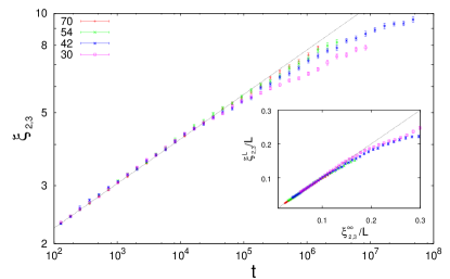
Figure 1: Time dependence of the coherence length for $T=1.263$ and all system sizes simulated. The line accounts for the power-law fit to $L=70$ data in the range $\xi_{2,3}\in[3,5]$, that corresponds to $\xi^{\infty}_{2,3}(t)\equiv 1.20(1)\,t^{1/7.44(10)}$. The inset shows the scaling function of the coherence length, evidencing the point where finite-size effects become important, $L\lesssim 6.5\,\xi_{2,3}(t)$.

In Fig. 1 we report the time dependence of $\xi_{2,3}(t)$ for various system sizes at $T=1.263$. In the early stage of the dynamics, in general for $\xi(t)\lesssim 3$, spatial correlation functions show the effects due to the lattice discretization and the growth of $\xi(t)$ shows some pre-asymptotic behavior. In the inset of Fig. 1 we show that finite-size effects come to play when $L\lesssim 6.5\,\xi_{2,3}(t)\simeq 7\xi(t)$, much earlier than the standard expectation, $\xi(t)\simeq L/2$. On top of the finite size effects, we also observe some deviations due to the uncertainty in estimating the contribution of the tail. As a consequence the estimation of the $z$ exponent from the fit $\xi_{2,3}(t)\,\propto\,t^{1/z}$ must be restricted to a time window that excludes both the short time dynamics (affected by lattice discretization) and the very long time dynamics, even for the largest volumes.

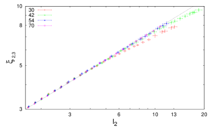
Figure 2: Data for $T=1.263$; different sizes have different number of data point, according to the length of the simulation shown in Table 1. The line corresponds to $\alpha=1.033$ obtained from fitting the $L=70$ data. Deviations from this line are finite size effects. Although the simulations for $L=42$ have been run longer for a factor 32, it is clear that the last part of the simulation is affected by strong finite size effects and practically useless for the estimation of the exponent.

Fortunately enough, all integrals $I_{k}$ experience the same inaccuracy in the extrapolation of the tail contribution, so that these errors compensate each other in the relation between $\xi_{k,k+1}$ and $I_{k}$. In Fig. 2 we clearly identify the finite size effects, but there are no other systematic errors due to the tail extrapolation. Since $I_{2}\,\propto\,\xi_{k,k+1}^{3-\alpha}$ we can extract the replicon exponent from a direct fit to the relation (7), without discarding late time data for the largest sizes. We use a standard method for linear fits with errors in both coordinates Press et al. (1992).

In principle, we could have used other values for $k$ and $m$ in $\xi_{k,k+1}$ and $I_{m}$ appearing in the relation (7). The choice for $\xi_{2,3}$ and $I_{2}$ is justified because it brings the highest amount of points for the fits of $\xi_{k,k+1}(I_{k})$ to a power-law, namely from 20% to 50% less discarded short-time data. To keep consistency with the $\alpha$ estimation, we have chosen $\xi_{2,3}$ for the estimate of exponent $z$.

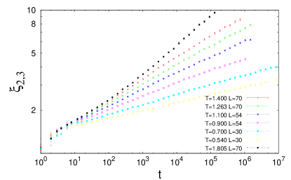
Figure 3: Time dependence of the coherence length $\xi_{2,3}$ for the largest size $L=70$ and several temperatures, ranging from the critical one $T_{c}=1.805$ down to very low temperatures.

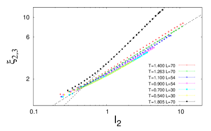
Figure 4: Data for $L=70$ and several temperatures. The relation $\xi_{2,3}\,\propto\,I_{2}^{1/(3-\alpha)}$ provides, at large times, a reliable estimate for the replicon exponent $\alpha$. Lines correspond to $\alpha=1.02$ for $T=1.263$ and $\alpha=1.77$ for $T=T_{c}=1.805$. The latter exponent corresponds to $\eta=-0.23(1)$, which is compatible with the latest estimate using equilibrium finite size scaling analysisJörg and Katzgraber (2008): $\eta=-0.275(25)$.

Table 3: Best estimates for the dynamical and replicon exponents from the fitting of the data shown in Fig. 3 and Fig. 4. The fits are performed on the range $[\xi_{\mathrm{min}},\xi_{\mathrm{max}}]$ for $z$, and with $\xi_{2,3}\geq\xi_{\mathrm{min}}$ in the case of $\alpha$. Errors are obtained through jackknife methods.

$T$	$[\xi_{\mathrm{min}},\xi_{\mathrm{max}}]$	$z$	$\chi^{2}_{\xi}$/d.o.f.	$\alpha$	$\chi^{2}_{I_{2}(\xi)}$/d.o.f.
1.805	[3.5,13.0]	4.95(04)	19/21	1.766(03)	3.4/21
1.400	[3.5,8.0]	6.86(14)	5.1/16	1.055(19)	1.5/18
	[4.0,8.0]	6.89(17)	3.3/14	1.050(22)	0.7/16
1.263	[3.0,5.0]	7.44(10)	6.2/11	1.020(10)	3.4/20
	[3.0,5.5]	7.45(08)	7.1/13
	[3.5,5.5]	7.46(10)	3.4/10	1.015(13)	2.1/17
1.100	[3.0,5.5]	9.15(15)	4.0/15	0.996(19)	7.8/20
	[3.5,5.5]	9.21(20)	3.4/11	1.024(29)	5.5/16
	[3.0,6.5]	9.19(16)	7.8/20
	[3.5,6.5]	9.23(27)	6.6/16
0.900	[2.7,4.0]	11.32(33)	6.6/14	0.909(31)	1.8/19
	[3.0,4.0]	11.50(46)	5.9/10	0.921(42)	1.4/15
0.700	[2.7,4.5]	15.31(67)	2.3/18	0.900(36)	1.1/18
	[3.0,4.5]	15.47(77)	1.3/14	0.923(40)	0.4/14
0.540	[2.3,3.3]	17.9(1.3)	12/17	0.896(39)	2.0/17
	[2.6,3.3]	19.6(2.1)	5.4/11	0.86(20)	1.8/11

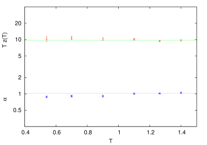
Figure 5: Best estimates for $z(T)$, multiplied by $T$, (above) and $\alpha$ (below) taken from Table 3. Lines are best fits: $Tz(T)=9.7(2)$ and $\alpha=1.025(9)$.

Our main results are summarized in Fig. 3 and Fig. 4 where $\xi_{2,3}(t)$ is shown as a function of time and $I_{2}(t)$, respectively, for several temperatures. From data in Fig. 3 we estimate the dynamical exponent $z$ by fitting to a power law in the range $\xi\in[\xi_{\mathrm{min}},\xi_{\mathrm{max}}]$, and from the data in Fig. 4 we get the replicon exponent $\alpha$ fitting in the range $\xi\geq\xi_{\mathrm{min}}$. It is immediately clear from the observation that all data with $T<T_{c}$ in Fig. 4 become parallel at large times that $\alpha$ is roughly constant in the low temperature phase. Our best estimates for the exponents $z$ and $\alpha$ are reported in Table 3, together with the fitting ranges, the corresponding $\chi^{2}$ and number of degree of freedom (d.o.f.). In Fig. 5 we plot the best estimate for the exponents $z$ and $\alpha$ in a way that makes evident that $z(T)\simeq 9.7(2)/T$ and $\alpha\simeq 1.025(9)$ for $T<T_{c}$. Actually the best value for $\alpha$ has been estimated only from data in the range $T\in[1,1.5]$, because for lower temperatures we observe a systematic decrease in the $\alpha$ value that we explain as follows. From data plotted in Fig. 4 we see that systems at the lowest temperatures are still approaching the asymptotic dynamics; so, it is likely that the small drift of the exponents for these low temperatures does not reflect a real change, but rather a preasymtotic effect due to a not large enough value of $\xi(t)$. Moreover in the $T=0$ limit we could have in principle a different exponent and we are maybe observing the beginning of the crossover region. Please note that the relatively small sizes used at lowest temperatures (see Table 1) do not induce any finite size effect, because the growth of $\xi(t)$ is extremely slow and barely reaches $\xi\sim 4<L/7$.

IV Conclusions

We have performed an extensive numerical study of the 4D Gaussian EA model with the aim of measuring the dynamical and the replicon exponents. We have used very large system sizes (up to $70^{4}$), which were never used before. These huge sizes are required to overcome finite size effects, which appear when the coherence length $\xi(t)$ is of the order of $1/7$ of the system size. The values of the replicon exponent $\alpha$, controlling the spatial decay of the correlation function, $C_{4}(r,t)\sim r^{-\alpha}$, are roughly constant in the low temperature region (apart from some pre-asymptotic effects at very low temperatures). Our final conservative estimate is $\alpha=1.03(2)$, which is not far, but definitely different from the one conjectured by the field theoretical arguments based on the analysis of the first order in the $\epsilon=6-d$ expansion, $(d-2+\eta)/2=0.883$. We also confirm that the dynamical exponent $z(T)$ is inversely proportional to the temperature in the entire temperature range we studied.

Appendix A A closer look on integral estimators

In this appendix we explore in some detail the properties of the integrals $I_{k}$ defined by Eq. (6) as well as the related estimators for the coherence length defined by Eq. (8). Note that the spin glass susceptibility is given by $\chi^{\mathrm{SG}}(t)=2\pi^{2}I_{3}(t)$. This relation offers a check for the correctness of the computation of the integrals. Since $\chi^{\mathrm{SG}}=N\overline{q^{2}}$ is a non self-averaging quantity we do such a comparison for the case in which we dispose the largest set of samples, see Fig. 6.

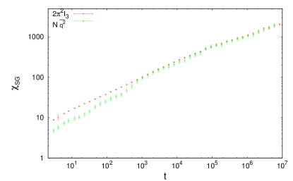
Figure 6: We check the reliability of the integral estimator $I_{3}$ comparing it to the SG susceptibility for the $L=30$ and $T=1.263$ case, where we have the largest number of samples (211).

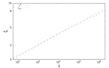
Figure 7: Comparison between the integral estimator for the coherence length, $\xi_{2,3}$, and the $\xi^{\mathrm{fit}}$ obtained by fitting to the Ansatz in Eq. (3). Data are for $L=70$, $T=1.263$ and the values of $\xi^{\mathrm{fit}}$ have been multiplied by a factor $1/\Gamma(4/3)=1.12$ in order to be equal to $\xi_{2,3}$ in case Ansatz in Eq. (3) is asymptotically exact. Fitting these data in the range $3<\xi<5$ we get $z(\xi_{2,3})=7.4(1)$ and $z(\xi^{\mathrm{fit}})=7.23(7)$. We draw a line of slope 1/7.3 as a guide for the eyes.

A comparison between the integral estimator $\xi_{2,3}$ for the coherence length and another estimator $\xi^{\mathrm{fit}}$ can be seen in Fig. 7. The latter is obtained by fitting correlation functions $C_{4}(r,t)$ with the Ansatz in Eq. (3) with $\alpha=1.0$ and $\delta=1.5$. These two estimators are in agreement with each other, once normalized according to Eq. (9). A closer inspection reveals the deviation of $\xi_{2,3}$ at larger times due to the badness of the estimation of the tail contribution, so that a secure range for a fit to obtain $z$ is $\xi_{2,3}\in[3,5]$, though compatible results are obtained in a wider time window, as can be seen in Table 3.