Spin echo dynamics under an applied drift field in graphene nanoribbon superlattices

Abstract

We investigate the evolution of spin dynamics in graphene nanoribbon superlattices (GNSLs) with armchair and zigzag edges in the presence of a drift field. We determine the exact evolution operator and show that it exhibits spin echo phenomena due to rapid oscillations of the quantum states along the ribbon. The evolution of the spin polarization is accompanied by strong beating patterns. We also provide detailed analysis of the band structure of GNSLs with armchair and zigzag edges.

Manipulation of electron spins using gate potentials in low dimensional semiconductor nanostructures is of interest, among other things, in that it provides a promising approach for the practical realization of robust qubit operations. Trauzettel et al. (2007); Wang et al. (2012a); Barnes and Das Sarma (2012); Wang et al. (2012b); Szumniak et al. (2013); Ban et al. (2012); Prabhakar et al. (2013a); Elzerman et al. (2004); Prabhakar et al. (2010); Shi et al. (2012) In recent years, experimental and theoretical research has sought a better understanding of the underlying physics of electrostatically defined quantum dots formed in two-dimensional electron gases for applications to solid state based quantum computing.Pryor and Flatté (2006); Flatté (2011); Prabhakar and Raynolds (2009); Prabhakar et al. (2011, 2012, 2013b); Amasha et al. (2008) In these devices, the spin-orbit interaction gives rise to decoherence due to the coupling of the electron spins to lattice vibrations. Hyperfine interactions between electron and nuclear spins are also a factor in some systems. Much work has focused on III-V systems although Si quantum dots Yang et al. (2013) are also of interest because of their relatively long decoherence times due to weak spin-orbit and hyperfine interactions. Shi et al. (2012) In another promising approach, experimentalists have succeeded in fabricating and testing a low operation voltage organic field effect transistor using graphene as the gate electrode placed over a thin polymer gate dielectric layer. Song et al. (2013) Graphene is promising because it exhibits extremely weak spin orbit coupling and hyperfine interactions. Min et al. (2006); Trauzettel et al. (2007); Recher et al. (2009); Recher and Trauzettel (2010); Allen et al. (2012); Fuchs et al. (2012); Krueckl and Richter (2012); Longhi (2012); Lim et al. (2012); Jung et al. (2012) In this paper, we present a theoretical investigation of the spin echo phenomena in GNSLs under an externally applied drift field. We find that the spin echo is accompanied by a strong beating pattern in the evolution of spin dynamics along the GNSLs with armchair and zigzag edges. We show that with a particular choice of the period and drift field, the spin polarization can be controlled to propagate on the surface of the Bloch sphere in a desired fashion.

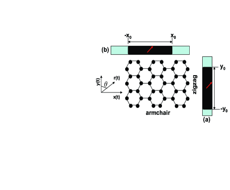
Figure 1: (Color online) Schematic diagram of graphene sheet with armchair along x-axis and zigzag along y-axis. Spin orientation shown by arrow sign in Fig. 1 (a) and (b) move rapidly between $-x_{0}$ and $+x_{0}$ for armchair and between $-y_{0}$ and $+y_{0}$ for zigzag GNSLs that induce spin echo under an externally applied drift field.

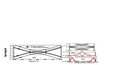
Figure 2: (Color online) Band structure of GNSLs with zigzag edge. Localized and edge states wave function squared are plotted in Fig. 2 (b) and (c) at $k=0.1\mathrm{nm^{-1}}$. Here we chose $U_{0}=+60~{}\mathrm{meV}$ for electron-like state and $U_{0}=-60~{}\mathrm{meV}$ for hole-like state. Also we chose $\Delta=60~{}\mathrm{meV}$, $v{{}_{{}_{F}}}=10^{4}~{}\mathrm{cm/s}$, $E_{D}=10^{6}~{}\mathrm{V/cm}$, $y_{0}=100~{}\mathrm{nm}$, $\ell_{0}=150~{}\mathrm{nm}$, $m=0.007m_{e}$ and $a=5~{}\mathrm{nm}$.

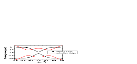
Figure 3: (Color online) Quasi-eigen energy of GNSLs with zigzag and armchair edges. The material parameters are chosen to be the same as in Fig. 2 but $E_{D}=10^{5}~{}\mathrm{V/cm}$ .

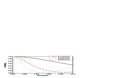
Figure 4: (Color online) Fidelity, $F=|\langle\chi_{-}|\chi\left(t\right)\rangle|$, vs time in GNSLs with zigzag edge. Here we chose $y_{0}=100~{}\mathrm{nm}$, $a=3~{}\mathrm{nm}$ and $\Delta=10~{}\mathrm{meV}$.

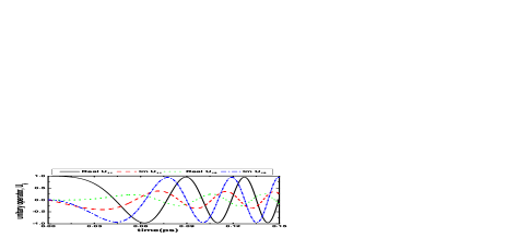
Figure 5: (Color online) Components of the evolution operator (exact results) for zigzag GNSLs under an applied drift field $E_{D}=1~{}\mathrm{mV/nm}$. The material constants are chosen to be the same as in Fig. 4.

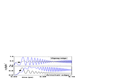
Figure 6: (Color online) Spin-flip transition probability vs time in both zigzag and armchair GNSLs at $a=1~{}\mathrm{nm}$ (solid lines with circles) and $a=3~{}\mathrm{nm}$ (solid lines). The material constants are chosen to be the same as in Fig. 4.

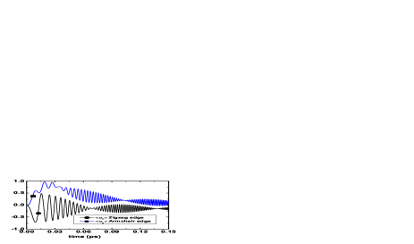
Figure 7: (Color online) Spin echo is observed in armchair and zigzag GNSLs under an externally applied drift field. Spin waves propagate in the form of temporal constructive and destructive interferences. Here we chose $x_{0}=y_{0}=100~{}\mathrm{nm}$, $E_{D}=10~{}\mathrm{mV/nm}$, $a=3~{}\mathrm{nm}$ and $\Delta=10~{}\mathrm{meV}$.

The effective mass Hamiltonian for single layer GNSLs elongated along either armchair or zigzag direction (see Fig. 1) near the K point of the Brillouin zone can be written as: $H=v{{}_{{}_{F}}}\bm{\sigma}\bm{\cdot}\mathbf{p}+\Delta\sigma_{z}+U(r,t)$. Here $v{{}_{{}_{F}}}$ is the Fermi velocity, $\Delta$ is the miniband width, $\sigma_{i}(i=x,y,z)$ are the Pauli spin matrices and $U\left(r,t\right)$ is the confining potential.

For GNSLs with zigzag edge, we consider $U(r,t)=U_{0}\left(y+y(t)\right)^{2}/\ell_{0}^{2}$ and the wave function of the above Hamiltonian $H$ is $\psi\left(x,y\right)=\exp{\left(ik_{x}x\right)\phi\left(y\right)}$ (see Ref. Castro Neto et al., 2009 for details). Now, we define the relative coordinate $Y=y-y(t)$ and relative momentum $P_{Y}=p_{y}-p_{y}\left(t\right)$ and formulate the total Hamiltonian in the form: $H=H\left(P_{Y},Y\right)+H_{qz}$. Here,

$$H\left(P_{Y},Y\right)=v{{}_{{}_{F}}}\sigma_{y}P_{Y}+U_{0}Y^{2}/\ell_{0}^{2},$$ (1)

$$H_{qz}=C_{1}\sigma_{x}+C_{2}\sin\left(k_{x}a\right)\sigma_{y}+\Delta\sigma_{z},$$ (2)

where $C_{1}=\hbar v{{}_{{}_{F}}}k_{x}$ and $C_{2}=v{{}_{{}_{F}}}my_{0}\alpha_{0}a$. Under an externally applied drift field $E_{D}$, we write the equation of motion for $k_{x}$ as: $\hbar\partial_{t}k_{x}(t)=eE_{D}$ (see Ref. Krueckl and Richter, 2012 for details). Thus we can write $k_{x}(t)=\alpha_{0}t$ with $\alpha_{0}=eE_{D}/\hbar$. In (2), we have written the quasi momentum $p_{y}(t)=m\dot{y}=-my_{0}\alpha_{0}a\sin\left(k_{x}(t)a\right)$. We have used the Finite Element Method and solved the corresponding eigenvalue problems for (1) and (2) and plotted the band structures of GNSLs with zigzag edge in Fig. 2(a). In addition to the localized states (Fig. 2 (b)), we also see the presence of edge states (Fig. 2 (c)) in GNSLs.

The Hamiltonian $H\left(P_{Y},Y\right)$ associated to the relative coordinates and relative momentum does not couple to the lowest spin states. Only the quasi-Hamiltonian $H_{qz}$ induces Bloch oscillations in the evolution of spin dynamics in GNSLs. Krueckl and Richter (2012) For convenience, we write Eq. (2) as:

$$H_{qz}(t)=Cs_{+}+C^{\star}s_{-}+2\Delta s_{z},$$ (3)

where $C=C_{1}-iC_{2}\sin\left(k_{x}(t)a\right)$, $C^{\star}=conj(C)$ and $s_{\pm}=s_{x}\pm is_{y}$. The band structures of quasi electron-hole states described by the Hamiltonian (3) can be written as

$$\delta=\pm\left[{|C|}^{2}+\Delta^{2}\right]^{1/2}.$$ (4)

The band structure of electron and hole states in the first Brillouin zone $[-\pi/a,\pi/a]$ with the specific choice of the parameters is shown in Fig. 3.

We construct a normalized orthogonal set of eigenspinors of the quasi-Hamiltonian (3) as:

$$\mathbf{\chi^{z}_{+}}\left(t\right)=\frac{\delta-\Delta}{\left[{{|C|}^{2}+\left(\delta-\Delta\right)^{2}}\right]^{1/2}}\left(\begin{array}[]{c}\frac{C}{\delta-\Delta}\\ 1\\ \end{array}\right),$$ (5)

$$\mathbf{\chi^{z}_{-}}\left(t\right)=\frac{\delta-\Delta}{\left[{{|C|}^{2}+\left(\delta-\Delta\right)^{2}}\right]^{1/2}}\left(\begin{array}[]{c}-1\\ \frac{C^{\star}}{\delta-\Delta}\\ \end{array}\right).$$ (6)

The above spinors (5) and (6) satisfy $\langle\chi^{z}_{+}|\chi^{z}_{+}\rangle=\langle\chi^{z}_{-}|\chi^{z}_{-}\rangle=1$ and $\langle\chi^{z}_{+}|\chi^{z}_{-}\rangle=\langle\chi^{z}_{-}|\chi^{z}_{+}\rangle=0$.

With the use of the Feynman disentangling technique, the exact evolution operator of Hamiltonian (3) can be written as (see also supplementary material sup, ):

$$U(t,0) = T\exp\left\{-\frac{i}{\hbar}\int H(t)dt\right\}$$ (7)

$$= \exp\left({\alpha(t)s_{+}}\right)\exp\left({\beta(t)s_{0}}\right)\exp\left({\gamma(t)s_{-}}\right),$$

where $T$ is the time ordering operator. At present, the time dependent functions $\alpha,\beta,\gamma$ are unknown and can be found by the Feynman disentangling scheme as discussed below. Feynman (1951); Popov (2007); Prabhakar et al. (2010, 2013a)

For a spin-1/2 particle, the exact evolution operator (7) can be written as:

$$U(t)=\left(\begin{array}[]{cc}\exp\left\{{\frac{\beta}{2}}\right\}+\alpha\gamma\exp\left\{{-\frac{\beta}{2}}\right\}&~{}~{}~{}\alpha\exp\left\{-{\frac{\beta}{2}}\right\}\\ \gamma\exp\left\{-{\frac{\beta}{2}}\right\}&~{}~{}~{}\exp\left\{-{\frac{\beta}{2}}\right\}\end{array}\right),$$ (8)

which can be seen to satisfy $U_{22}=\mathrm{conj}(U_{11})$ and $U_{12}=-\mathrm{conj}(U_{21})$ due to the fact that $U(t)$ is unitary.

At $t=0$, we use the initial condition $\chi^{z}\left(0\right)=\left(0~{}1\right)^{\top}$, where $\top$ denotes transpose and write $\chi^{z}\left(t\right)=U(t,0)\chi^{z}\left(0\right)$ as

$$\chi^{z}\left(t\right)=\left(\alpha\exp\left\{-\beta/2\right\}~{}~{}\exp\left\{-\beta/2\right\}\right)^{\top}.$$ (9)

Next, we find the functional form of $\alpha(t)$, $\beta(t)$, and $\gamma(t)$ of GNSLs with zigzag edge by utilizing the Feynman disentangling scheme. Feynman (1951); Popov (2007); Prabhakar et al. (2010, 2013a)

The exact evolution operator of Hamiltonian (3) can be written as:

$$U(t) = \exp{\left\{\alpha(t)s_{+}\right\}}T$$ (10)

$$\exp\left[-\frac{i}{\hbar}\int_{0}^{t}\left\{\left(C-x\right)s^{\prime}_{+}+C^{\star}s^{\prime}_{-}+2\Delta s^{\prime}_{0}\right\}dt^{\prime}\right],~{}~{}~{}~{}~{}~{}$$

where

$$\alpha\left(t\right)=-\frac{i}{\hbar}\int^{t}_{0}x(t)dt^{\prime},$$ (11)

$$s^{\prime}_{\mu}\left(t\right)=\exp\left(-\alpha s_{+}\right)s_{\mu}\exp\left(\alpha s_{+}\right).$$ (12)

Differentiating Eq. (12) with respect to $\alpha$, we find

$$\frac{ds^{\prime}_{\mu}\left(t\right)}{d\alpha}=-\exp\left(-\alpha s_{+}\right)\left(s_{+}s_{\mu}-s_{\mu}s_{+}\right)\exp\left(\alpha s_{+}\right).$$ (13)

By utilizing initial condition $s^{\prime}_{\mu}\left(0\right)=s_{\mu}$, the primed operators are determined

$$s^{\prime}_{+}=s_{+},~{}s^{\prime}_{0}=s_{+}\alpha+s_{0},~{}s^{\prime}_{-}=s_{-}-s_{+}\alpha^{2}-2s_{0}\alpha.$$ (14)

By substituting Eq. (14) in Eq. (10) and equating the coefficient of $s_{+}$ to zero, we find the following Riccatti equation:

$$\frac{d\alpha}{dt}=-\frac{i}{\hbar}\left\{C-C^{\star}\alpha^{2}+2\Delta\alpha\right\}.$$ (15)

Hence the dependence on $s_{+}$ in (10) has been disentangled. By following the above procedure and by disentangling $s_{0}$ and $s_{-}$, another set of the Riccatti equations for the time dependent functions $\beta(t)$ and $\gamma(t)$ can be written as

$$\frac{d\beta}{dt}=-\frac{2i}{\hbar}\left\{\Delta-C^{\star}\alpha\right\},$$ (16)

$$\frac{d\gamma}{dt}=-\frac{i}{\hbar}C^{\star}\exp\left\{\beta\right\}.$$ (17)

In a similar way, for armchair GNSLs, we write the total Hamiltonian $H=H\left(P_{X},X\right)+H_{qa}$, where

$$H\left(P_{X},X\right)=v{{}_{{}_{F}}}\sigma_{x}P_{x}+U_{0}X^{2}/\ell_{0}^{2},$$ (18)

$$H_{qa}=-C^{\prime}_{2}\cos\left(k_{y}(t)a\right)\sigma_{x}+C^{\prime}_{1}\sigma_{y}+\Delta\sigma_{z}.$$ (19)

Here $C_{1}^{\prime}=\hbar v{{}_{{}_{F}}}k_{y}(t)$ and $C_{2}^{\prime}=v{{}_{{}_{F}}}mx_{0}\alpha_{0}a$. We construct a normalized orthogonal set of eigenspinors of the quasi-Hamiltonian (19) as:

$$\mathbf{\chi^{a}_{+}}\left(t\right)=\frac{\delta-\Delta}{\left[{{|C^{\prime}|}^{2}+\left(\delta-\Delta\right)^{2}}\right]^{1/2}}\left(\begin{array}[]{c}-1\\ \frac{-i{C^{\prime}}^{\star}}{\Delta-\delta}\\ \end{array}\right),$$ (20)

$$\mathbf{\chi^{a}_{-}}\left(t\right)=\frac{\delta-\Delta}{\left[{{|C^{\prime}|}^{2}+\left(\delta-\Delta\right)^{2}}\right]^{1/2}}\left(\begin{array}[]{c}\frac{iC^{\prime}}{\Delta-\delta}\\ 1\\ \end{array}\right),$$ (21)

where $C^{\prime}=C^{\prime}_{1}-iC^{\prime}_{2}\cos\left(a\alpha_{0}t\right)$. At $t=0$, we use the initial condition

$$\mathbf{\chi^{a}}\left(0\right)=\frac{\delta-\Delta}{\left[C_{2}^{\prime 2}+\left(\delta-\Delta\right)^{2}\right]^{1/2}}\left(\begin{array}[]{c}\frac{C^{\prime}_{2}}{\Delta-\delta}\\ 1\\ \end{array}\right),$$ (22)

and find $\chi^{a}\left(t\right)=U(t,0)\chi^{a}\left(0\right)$. The three coupled Riccatti equations for the quasi-Hamiltonian of GNSLs with armchair edge can be written as

$$\frac{d\alpha}{dt}=-\frac{i}{\hbar}\left\{\tilde{C}-{\tilde{C}}^{\star}\alpha^{2}+2\Delta\alpha\right\},$$ (23)

$$\frac{d\beta}{dt}=-\frac{2i}{\hbar}\left\{\Delta-{\tilde{C}}^{\star}\alpha\right\},$$ (24)

$$\frac{d\gamma}{dt}=-\frac{i}{\hbar}{\tilde{C}}^{\star}\exp\left\{\beta\right\},$$ (25)

where $\tilde{C}=-iC^{\prime}$. We have solved the three coupled Riccatti equations for zigzag and armchair GNSLs numerically and found the exact evolution operator (8). The supplementary material provides an additional example of finding exact evolution operator for a spin-1/2 particle in presence of tilted magnetic field. sup

In Fig. 4, we have plotted the fidelity vs time for several different values of the applied drift field. As expected from the analytical solutions (see Eqs. 6 and 9), with the increasing drift field, the fidelity becomes enhanced because the amplitude of the spin polarization increases as the magnitude of the applied drift field is increased while the spatial frequency of the propagating waves is reduced. These effects cause dips in fidelity at an early stage with increasing magnitude of the drift field.

In Fig. 5, we study the evolution operator in graphene under a drift field. The components of $U_{ij}$ are superposed leading to constructive and destructive interferences. We observe Hahn echo patterns in a constructive interference regime of the evolution of spin dynamics.Belonenko et al. (2012); Hahn (1950) This will be separately discussed with reference to Fig. 7. Spin flip occurs when the localized states in GNSLs with armchair and zigzag edges move rapidly along the ribbon with the application of the time dependent gate controlled electric field. Such spin flip probabilities are plotted in Fig. 6 for both the armchair and zigzag GNSLs at different values of the period of the superlattices. As can be seen, the spin-flip probabilities in both the armchair and zigzag GNSLs are enhanced with increasing value of the period of the superlattice. This is due to the fact that the enhancement in the amplitude of the spin waves occur with the increasing value of the period of the superlattice.

In Fig. 7, we have plotted the expectation values of the Pauli spin matrices vs time under an externally applied drift field in both GNSLs with zigzag and armchair edges. For $t>0$, the components of the spin waves fluctuate rapidly and thus we observed Hahn echo patterns in GNSLs. In this regime, where the spin echo can be observed, the spin waves are superposed which induce constructive interference. When the superposed spin waves induce destructive interference, we find strong beating patterns. The Hahn echo accompanied by strong beating patterns can be seen at different intervals of time in GNSLs with zigzag (solid line with circles) and armchair (solid lines with diamond) edges due to the fact that the spin waves in both kinds of superlattices travel with different velocities. Note that the Hahn echo patterns in $\langle\sigma_{x}\rangle$ of zigzag edge resemble to the $\langle\sigma_{y}\rangle$ of armchair edge. This is due to the fact that the coefficients of $\sigma_{x}$ and $\sigma_{y}$ of the quasi-Hamiltonian of the GNSLs with zigzag and armchair edges Eq. (2) and (19) respectively interchanges during the evolution of spin dynamics.

To conclude, we have shown that the quasi-Hamiltonian of the GNSLs with zigzag and armchair edges can be used to investigate the evolution of spin dynamics under an externally applied drift field. We have shown that the exact evolution operator can be found for such Hamiltonian via the Feynman disentangling technique. With a particular choice of the period and drift field, the spin polarization can be controlled to propagate on the surface of the Bloch sphere in a desired fashion. During the transportation of the spin on the surface of the Bloch sphere, the Hahn echo, accompanied by strong beating patterns, is observed. The authors in Ref. Song et al., 2013 have fabricated a field effect transistors (FET) using graphene where the gate electrode was placed over a thin polymer gate dielectric layer. Such devices show excellent output and transfer characteristics (mobility $\approx 0.1\mathrm{cm^{2}/Vs}$) for gate and drain operations (see Fig.(4b) in Ref. Song et al., 2013). The present work was motivated in part by these experimental studies and our results (e.g., Figs. 1-7) might provide useful information for the design of quantum logic gates based on the application of the externally applied drift fields in GNSLs with both the armchair and zigzag edges.

This work has been supported by NSERC (Canada) and Canada Research Chair programs.

Supplementary materials:

To verify that the evolution operator (Eq. 8) is exact, we provide an example associated with the Hamiltonian of spin-1/2 particle in an effective magnetic field having a known solution: Griffiths (1995)

$$H(t)=\Omega\cos\left(\omega t\right)s_{x}+\Omega\sin\left(\omega t\right)s_{y}+\Delta s_{z}.$$ (26)

The energy eigenvalues of (26) are $\varepsilon_{\pm}=\pm\hbar\delta/2,$ where $\delta=\left[\Delta^{2}+\Omega^{2}\right]^{1/2}$. We construct a normalized orthogonal set of eigenspinors of Hamiltonian (26) as:

$$\mathbf{\chi_{+}}\left(t\right)=\frac{1}{\sqrt{N}}\left(\begin{array}[]{c}\Omega\\ \left(\delta-\Delta\right)\exp\left\{i\omega t\right\}\\ \end{array}\right),$$ (29)

$$\mathbf{\chi_{-}}\left(t\right)=\frac{1}{\sqrt{N}}\left(\begin{array}[]{c}\left(\delta-\Delta\right)\exp\left\{-i\omega t\right\}\\ -\Omega\\ \end{array}\right),$$ (32)

where

$$N^{2}=\Omega^{2}+\left(\delta-\Delta\right)^{2}.$$ (33)

Since the Hamiltonian (26) is time dependent, the general time dependent Schrödinger equations can be written as

$$\partial_{t}a(t)=-\frac{i}{2}\left(\Delta a+\Omega\exp\left\{-i\omega t\right\}b\right),$$ (34)

$$\partial_{t}b(t)=-\frac{i}{2}\left(\Omega\exp\left\{i\omega t\right\}a-\Delta b\right).$$ (35)

The exact solution of time dependent Schrödinger Eqs. (34) and (35) can be written as: Griffiths (1995)

$$a\left(t\right)=\frac{\Omega}{\sqrt{N}}\left\{\cos\left(\frac{\lambda^{\prime}t}{2}\right)-\frac{i}{\lambda^{\prime}}\left(\delta-\omega\right)\sin\left(\frac{\lambda^{\prime}t}{2}\right)\right\}\exp\left(-\frac{i\omega t}{2}\right),$$ (36)

$$b\left(t\right)=\frac{\delta-\Delta}{\sqrt{N}}\left\{\cos\left(\frac{\lambda^{\prime}t}{2}\right)-\frac{i}{\lambda^{\prime}}\left(\delta+\omega\right)\sin\left(\frac{\lambda^{\prime}t}{2}\right)\right\}\exp\left(\frac{i\omega t}{2}\right),$$ (37)

where

$$\lambda^{\prime}=\sqrt{\Omega^{2}+\left(\Delta-\omega\right)^{2}}.$$ (38)

Expressing (36) and (37) as a linear combination of $|\chi_{+}\rangle$ and $|\chi_{-}\rangle$, we have

$$\psi\left(t\right)=\left\{\cos\left(\frac{\lambda^{\prime}t}{2}\right)-\frac{i}{\lambda^{\prime}}\left(\delta-\frac{\omega\Delta}{\delta}\right)\sin\left(\frac{\lambda^{\prime}t}{2}\right)\right\}\exp\left(-\frac{i\omega t}{2}\right)\chi_{+}\left(t\right)+i\frac{\omega\Omega}{\lambda^{\prime}\delta}\sin\left(\frac{\lambda^{\prime}t}{2}\right)\exp\left(\frac{i\omega t}{2}\right)\chi_{-}\left(t\right).$$ (39)

Clearly, one can immediately write the transition probability:

$$|\langle\chi_{-}\left(t\right)|\psi\left(t\right)\rangle|^{2}=\left(\frac{\omega\Omega}{\lambda^{\prime}\delta}\right)^{2}\sin^{2}\left(\frac{\lambda^{\prime}t}{2}\right),\\$$ (40)

provided that

$$|\langle\chi_{-}\left(t\right)|\psi\left(t\right)\rangle|^{2}+|\langle\chi_{+}\left(t\right)|\chi\left(t\right)\rangle|^{2}=1.$$ (41)

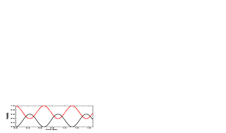
Figure 8: (Color online) Transition probability vs time. Here we chose $\omega=10~{}\mathrm{THz}$ and $\Omega=\Delta=1~{}\mathrm{THz}$. Transition probabilities obtained from Eqs. (40) and (41) (solid and dashed lines, respectively) are seen to be in excellent agreement to the ones obtained from the Feynman disentangling operator scheme. The transition probabilities are given by $|\langle\chi_{+}\left(t\right)|U\left(t,0\right)\chi\left(0\right)\rangle|^{2}$ (circles) and $|\langle\chi_{-}\left(t\right)|U\left(t,0\right)\chi\left(0\right)\rangle|^{2}$ (triangles).

Next, we apply the Feynman disentangling operator scheme and find the exact evolution operator of the Hamiltonian (26) which initially takes the form of (Eq.9, see the paper) but with three different coupled Riccati equations (evolved during the disentangling operator scheme of the Hamiltonian (26)). These are:

$$\frac{d\alpha}{dt}=-\frac{i}{\hbar}\left\{\frac{\Omega}{2}\exp\left(-i\omega t\right)+\Delta\alpha-\frac{\Omega}{2}\exp\left(i\omega t\right)\alpha^{2}\right\},~{}~{}~{}~{}$$ (42)

$$\frac{d\beta}{dt}=-\frac{i}{\hbar}\left\{\Delta-\Omega\exp\left(i\omega t\right)\alpha\right\},~{}~{}~{}~{}~{}~{}$$ (43)

$$\frac{d\gamma}{dt}=-\frac{i}{\hbar}\frac{\Omega}{2}\exp\left\{\beta+i\omega t\right\}.~{}~{}~{}~{}~{}~{}$$ (44)

Usually, an exact solution of such Riccati differential equations does not exist. However, in this case, it is possible to find the exact solution of Eqs. (42), (43) and (44) as:

$$\alpha\left(t\right)=\frac{\exp\left(-i\lambda t\right)-\exp\left(-i\omega t\right)}{n_{2}-n_{1}\exp\left(-i\varpi t\right)},$$ (45)

$$\beta\left(t\right)=\frac{\exp\left(-i\lambda t\right)\left(n_{2}-n_{1}\right)^{2}}{\left\{n_{2}-n_{1}\exp\left(-i\varpi t\right)\right\}^{2}},$$ (46)

$$\gamma\left(t\right)=\frac{\exp\left(-i\varpi t\right)-1}{n_{2}-n_{1}\exp\left(-i\varpi t\right)},$$ (47)

where $\lambda=\varpi+\omega$, $\varpi=\Omega\left(n_{2}-n_{1}\right)/2$,

$$n_{1}=\frac{\Delta-\omega}{\Omega}+\frac{\left[\left(\Delta-\omega\right)^{2}+\Omega^{2}\right]^{1/2}}{\Omega},$$ (48)

$$n_{2}=\frac{\Delta-\omega}{\Omega}-\frac{\left[\left(\Delta-\omega\right)^{2}+\Omega^{2}\right]^{1/2}}{\Omega}.$$ (49)

In Fig. 8, the transition probability obtained from Eqs. (40) and (41) (solid and dashed lines) is seen to be in excellent agreement to the one obtained from the disentangling scheme (circles and triangles). Thus, we have demonstrated that the evolution operator obtained from the disentangling operator scheme is exact. Finding an exact unitary operator is one of the requirements for quantum computing and is one of the motivations of the present work.

References

Trauzettel et al. (2007)B. Trauzettel, D. V. Bulaev, D. Loss, and G. Burkard, Nat Phys 3, 192 (2007).
Prabhakar et al. (2013a)S. Prabhakar, R. Melnik, and L. L. Bonilla, Journal of Physics
D: Applied Physics 46, 265302 (2013a).
Elzerman et al. (2004)J. M. Elzerman, R. Hanson,
L. H. Willems van
Beveren, B. Witkamp,
L. M. K. Vandersypen, and L. P. Kouwenhoven, Nature 430, 431 (2004).
Prabhakar et al. (2010)S. Prabhakar, J. Raynolds,
A. Inomata, and R. Melnik, Phys. Rev. B 82, 195306 (2010).
Shi et al. (2012)Z. Shi, C. B. Simmons,
J. R. Prance, J. K. Gamble, T. S. Koh, Y.-P. Shim, X. Hu, D. E. Savage, M. G. Lagally, M. A. Eriksson, M. Friesen, and S. N. Coppersmith, Phys. Rev. Lett. 108, 140503 (2012).
Amasha et al. (2008)S. Amasha, K. MacLean,
I. P. Radu, D. M. Zumbühl, M. A. Kastner, M. P. Hanson, and A. C. Gossard, Phys. Rev. Lett. 100, 046803 (2008).
Yang et al. (2013)C. H. Yang, A. Rossi,
R. Ruskov, N. S. Lai, F. A. Mohiyaddin, S. Lee, C. Tahan, G. Klimeck, A. Morello, and A. S. Dzurak, Nat Commun 4, 2069 (2013).
Song et al. (2013)J. Song, F.-Y. Kam,
R.-Q. Png, W.-L. Seah, J.-M. Zhuo, G.-K. Lim, P. K. H. Ho, and L.-L. Chua, Nat Nano 8, 356 (2013).
Min et al. (2006)H. Min, J. E. Hill,
N. A. Sinitsyn, B. R. Sahu, L. Kleinman, and A. H. MacDonald, Phys.
Rev. B 74, 165310
(2006).