Modified melting crystal model and Ablowitz-Ladik hierarchy

Abstract

This is a review of recent results on the integrable structure of the ordinary and modified melting crystal models. When deformed by special external potentials, the partition function of the ordinary melting crystal model is known to become essentially a tau function of the 1D Toda hierarchy. In the same sense, the modified model turns out to be related to the Ablowitz-Ladik hierarchy. These facts are explained with the aid of a free fermion system, fermionic expressions of the partition functions, algebraic relations among fermion bilinears and vertex operators, and infinite matrix representations of those operators.

1 Introduction

Recently, we extended our previous work [1, 2] on the integrable structure of the melting crystal model — a model of random 3D Young diagrams — to a modified model [3, 4]. In the context of string theory [5], the modified model is related to topological string theory on the so called resolved conifold. Our study was motivated by Brini’s conjecture [6] that all genus Gromov-Witten invariants of this non-compact complex Calabi-Yau 3-fold can be captured by the Ablowitz-Ladik hierarchy [7]. Brini confirmed his conjecture to the first order (i.e., genus $\leq 1$) of genus expansion. Proving the conjecture in the full genus case remained open. We believe that our results show an affirmative answer (or, at least, a decisive piece of evidence) to this question.

In our previous work [1, 2], the partition function of the melting crystal model is shown to be related to a tau function of the 1D Toda hierarchy. This fact is proven with the aid of a free fermion system, a fermionic realization of the quantum torus algebra, and algebraic relations called shift symmetries in this algebra. We could use these tools for the modified model as well to show that the partition function is related to a tau function of the 2D Toda hierarchy [3]. Although this was an important step, a new technique was wanted to reach the goal.

A final clue was found in the work of Brini et al. [8]. They presented a characterization of the Ablowitz-Ladik hierarchy (or, rather, the relativistic Toda hierarchy ) in the Lax formalism of the 2D Toda hierarchy. According to the characterization by Brini et al., the Ablowitz-Ladik hierarchy amounts to the case where the Lax operators of the 2D Toda hierarchy have a special quotient (or rational) form. We examined the Lax operators of the aforementioned tau function, and confirmed that they do have the special form [4].

2 Melting crystal model

2.1 Crystal corner, 3D Young diagrams and plane partitions

The melting crystal model is a statistical model of a crystal corner (Figure 2). The crystal consists of unit cubes and occupies an octant of the $xyz$ space. The complement of the crystal in the octant is a 3D Young diagram, which conversely determines the shape of the crystal (Figure 2).

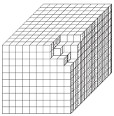
Figure 1: Melting crystal corner

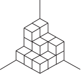
Figure 2: 3D Young diagram

Just as ordinary Young diagrams are identified with ordinary partitions

$$\lambda=(\lambda_{i})_{i=1}^{\infty},\quad\lambda_{1}\geq\lambda_{2}\geq\ldots\geq 0,\quad|\lambda|=\sum_{i=1}^{\infty}\lambda_{i}<\infty,$$

of integers [11], 3D Young diagrams are in one-to-one correspondence with plane partitions. Plane partitions are 2D arrays of non-negative integers that are decreasing in two directions:

$$\pi=(\pi_{ij})_{i,j=1}^{\infty}=\left(\begin{array}[]{ccc}\pi_{11}&\pi_{12}&\cdots\\ \pi_{21}&\pi_{22}&\cdots\\ \vdots&\vdots&\ddots\end{array}\right),\quad\begin{array}[]{ccc}\pi_{ij}&\geq&\pi_{i,j+1}\\ \mbox{\rotatebox[origin={c}]{-90.0}{$\geq$}}&&\\ \pi_{i+1,j}&&\end{array},\quad|\pi|=\sum_{i,j=1}^{\infty}\pi_{ij}<\infty.$$

Such a plane partition determines a 3D Young diagram that consists of stacks of unit cubes of height $\pi_{ij}$ on the unit squares $[i-1,i]\times[j-1,j]$, $i,j=1,2,\ldots$, of the $xy$ plane. For example, the 3D Young diagram of Figure 2 corresponds to

$$\pi=\left(\begin{array}[]{ccc}3&2&2\\ 3&2&1\\ 1&1&1\end{array}\right).$$

The partition function of this model is the sum

$$Z=\sum_{\pi\in\mathcal{P}\mathcal{P}}q^{|\pi|}$$ (3)

of the Boltzmann weight $q^{|\pi|}$ ($0<q<1$) over the set $\mathcal{P}\mathcal{P}$ of all plane partitions.

2.2 Method of diagonal slicing

The partition function (3) can be calculated by the method of diagonal slicing [12]. Let us define the $m$-th diagonal slice $\pi(m)$, $m\in\mathbf{Z}$, of $\pi$ as

$$\pi(m)=\begin{cases}(\pi_{i,i+m})_{i=1}^{\infty}&\mbox{if $m\geq 0$},\\ (\pi_{j-m,j})_{j=1}^{\infty}&\mbox{if $m<0$}.\end{cases}$$

$\pi(m)$ represents the slice of the 3D Young diagram along the vertical plane $y=x+m$ (Figure 4). The two sets $\{\pi(-m)\}_{m=0}^{\infty}$ and $\{\pi(m)\}_{m=0}^{\infty}$ of these slices give two increasing sequences of Young diagrams that fill up the Young diagram of shape $\lambda=\pi(0)$.

These increasing sequences of Young diagrams can be encoded to semi-standard tableaux $T,T^{\prime}$ of shape $\lambda$ [11]. These tableaux are obtained by entering the numbers $m+1$, $m=0,1,2,\ldots$, to the boxes of the skew Young diagrams $\pi(-m)/\pi(-m-1)$ and $\pi(m)/\pi(m+1)$ (Figure 4). It is easy to see that the entries $T(i,j)$ and $T^{\prime}(i,j)$ of $T,T^{\prime}$ satisfy the conditions

$$\begin{array}[]{ccc}T(i,j)&\geq&T(i,j+1)\\ \mbox{\rotatebox[origin={c}]{-90.0}{$>$}}&&\\ T(i+1,j)&&\end{array},\quad\begin{array}[]{ccc}T^{\prime}(i,j)&\geq&T^{\prime}(i,j+1)\\ \mbox{\rotatebox[origin={c}]{-90.0}{$>$}}&&\\ T^{\prime}(i+1,j)&&\end{array}$$ (10)

that characterize semi-standard tableaux . Thus any plane partition $\pi$ determines a triple $(\lambda,T,T^{\prime})$ of a partition $\lambda$ and semi-standard tableaux $T,T^{\prime}$ of shape $\lambda$. It is also easy to see that any such triple determine a plane partition. The mapping $\pi\to(\lambda,T,T^{\prime})$ thus turns out to be a bijection between $\mathcal{P}\mathcal{P}$ and the set of all triples.

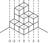
Figure 3: Diagonal slices

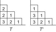
Figure 4: Semi-standard tableaux

The sum in (3) can be thus converted to a sum over $(\lambda,T,T^{\prime})$’s. Moreover, the weight $q^{|\pi|}$ can be factorized as

$$q^{|\pi|}=q^{T}q^{T^{\prime}},\quad q^{T}=\prod_{m=0}^{\infty}q^{(m+1/2)|\pi(-m)/\pi(-m-1)|},\quad q^{T^{\prime}}=\prod_{m=0}^{\infty}q^{(m+1/2)|\pi(m)/\pi(m+1)|}.$$ (11)

Because of this factorization, the sum in (3) can be separated to partial sums with respect to $T,T^{\prime}$ and a sum with respect to $\lambda$ as

$$Z=\sum_{\lambda\in\mathcal{P}}\left(\sum_{T:\;\mathrm{shape}\;\lambda}q^{T}\right)\left(\sum_{T^{\prime}:\;\,\mathrm{shape}\;\lambda}q^{T^{\prime}}\right),$$

where $\mathcal{P}$ denotes the set of all partitions. According to the combinatorial definition

$$s_{\lambda}(\boldsymbol{x})=\sum_{T:\;\mathrm{shape}\;\lambda}\boldsymbol{x}^{T},\quad\boldsymbol{x}^{T}=\prod_{(i,j)}x_{T(i,j)},$$ (12)

of Schur functions of $\boldsymbol{x}=(x_{1},x_{2},\ldots)$ [11], the partial sums over $T,T^{\prime}$ become a special value of $s_{\lambda}(\boldsymbol{x})$:

$$\sum_{T:\;\mathrm{shape}\;\lambda}q^{T}=\sum_{T^{\prime}:\;\mathrm{shape}\;\lambda}q^{T^{\prime}}=s_{\lambda}(q^{-\rho}),\quad q^{-\rho}=\left(q^{1/2},q^{3/2},\ldots,q^{k+1/2},\ldots\right).$$ (13)

The partition function can be thus reduced to a sum over $\mathcal{P}$:

$$Z=\sum_{\lambda\in\mathcal{P}}s_{\lambda}(q^{-\rho})^{2}.$$ (14)

One can now use the Cauchy identity [11]

$$\sum_{\lambda\in\mathcal{P}}s_{\lambda}(x_{1},x_{2},\ldots)s_{\lambda}(y_{1},y_{2},\ldots)=\prod_{i,j=1}^{\infty}(1-x_{i}y_{j})^{-1}$$ (15)

to calculate (14) explicitly:

$$Z=\sum_{\lambda\in\mathcal{P}}s_{\lambda}(q^{-\rho})^{2}=\prod_{i,j=1}^{\infty}(1-q^{i+j-1})^{-1}=\prod_{n=1}^{\infty}(1-q^{n})^{-n}.$$ (16)

This function is known as the MacMahon function.

2.3 Deformations by external potentials

A simplest deformation of this model is obtained by inserting the extra weight $Q^{|\pi(0)|}$, where $Q$ is a new positive constant. The foregoing partition function (3) is thereby deformed as

$$Z=\sum_{\pi\in\mathcal{P}\mathcal{P}}q^{|\pi|}Q^{|\pi(0)|}.$$ (17)

This is a deformation induced by the external potential $|\pi(0)|\log Q$. By the mapping $\pi\mapsto(\lambda,T,T^{\prime})$, this sum, too, can be reduced to a sum of the form

$$Z=\sum_{\lambda\in\mathcal{P}}s_{\lambda}(q^{-\rho})^{2}Q^{|\lambda|},$$ (18)

and eventually boils down to a generalization of the MacMahon function:

$$Z=\prod_{i,j=1}^{\infty}(1-Qq^{i+j-1})^{-1}=\sum_{n=1}^{\infty}(1-Qq^{n})^{-n}.$$ (19)

An integrable hierarchy emerges in a deformed partition function $Z(s,\boldsymbol{t})$ that depends on a discrete variable $s\in\mathbf{Z}$ and a set of continuous variables $\boldsymbol{t}=(t_{1},t_{2},\ldots)$. The deformations are induced by the external potential

$$\Phi(\lambda,s,\boldsymbol{t})=\sum_{k=1}^{\infty}t_{k}\Phi_{k}(\lambda,s),\quad\Phi_{k}(\lambda,s)=\sum_{i=1}^{\infty}(q^{k(\lambda_{i}+s-i+1)}-q^{k(s-i+1)})+\frac{1-q^{ks}}{1-q^{k}}q^{k}.$$ (20)

Note that the sum in the definition of $\Phi_{k}(\lambda,s)$ is actually a finite sum. This expression is an analytic continuation of the expression

$$\Phi_{k}(\lambda,s)=\sum_{i=1}^{\infty}q^{k(\lambda_{i}+s-i+1)}-\sum_{i=1}^{\infty}q^{k(-i+1)}$$ (21)

in the domain $|q|>1$ of the $q$-plane. The term $Q^{|\lambda|}$ in (18), too, has to be replaced by the $s$-dependent form $Q^{|\lambda|+s(s+1)/2}$. With the aid of 2D complex free fermion system (which will be briefly reviewed in the next section), we obtained the following result [1, 2]:

Theorem 1.

The deformed partition function

$$Z(s,\boldsymbol{t})=\sum_{\lambda\in\mathcal{P}}s_{\lambda}(q^{-\rho})^{2}Q^{|\lambda|+s(s+1)/2}e^{\Phi(\lambda,s,\boldsymbol{t})}$$ (22)

is related to a special tau function $\tau(s,\boldsymbol{t})$ of the 1D Toda hierarchy as

$$Z(s,\boldsymbol{t})=\exp\left(\sum_{k=1}^{\infty}\frac{t_{k}q^{k}}{1-q^{k}}\right)q^{-s(s+1)(2s+1)/6}\tau(s,\iota(\boldsymbol{t})),$$ (23)

where $\iota(\boldsymbol{t})$ denotes the alternating inversion

$$\iota(\boldsymbol{t})=(-t_{1},t_{2},-t_{3},\ldots,(-1)^{k}t_{k},\ldots)$$

of $\boldsymbol{t}=(t_{1},t_{2},\ldots)$.

3 Modified melting crystal model

3.1 Partition function

The modified model is obtained by replacing

$$s_{\lambda}(q^{-\rho})^{2}\;\to\;s_{\lambda}(q^{-\rho})s_{\>{}^{\mathrm{t}}\lambda}(q^{-\rho}),$$

where $\>{}^{\mathrm{t}}\lambda$ denotes the conjugate partition that represents the transpose of the associated Young diagram. The $Q$-dependent partition function reads

$$Z^{\prime}=\sum_{\lambda\in\mathcal{P}}s_{\lambda}(q^{-\rho})s_{\>{}^{\mathrm{t}}\lambda}(q^{-\rho})Q^{|\lambda|}.$$ (24)

This is no longer a statistical model of 3D Young diagrams. $s_{\lambda}(q^{-\rho})$ and $s_{\>{}^{\mathrm{t}}\lambda}(q^{-\rho})$ are partial sums of contributions from “half” pieces of 3D Young diagrams, but these pieces cannot be glued along the plane $x=y$. By the Cauchy identity

$$\sum_{\lambda\in\mathcal{P}}s_{\lambda}(x_{1},x_{2},\ldots)s_{\>{}^{\mathrm{t}}\lambda}(y_{1},y_{2},\ldots)=\prod_{i,j=1}^{\infty}(1+x_{i}y_{j})$$ (25)

of another type [11], one can convert (24) to an infinite product of the form

$$Z^{\prime}=\sum_{i,j=1}^{\infty}(1+Qq^{i+j-1})=\prod_{n=1}^{\infty}(1+Qq^{n})^{n}.$$ (26)

We deform (24) by the external potential

$$\Phi(\lambda,s,\boldsymbol{t},\bar{\boldsymbol{t}})=\sum_{k=1}^{\infty}t_{k}\Phi_{k}(\lambda,s)+\sum_{k=1}^{\infty}\bar{t}_{k}\Phi_{-k}(\lambda,s)$$

that depends on a discrete variable $s$ and two sets of continuous variables $\boldsymbol{t}=(t_{1},t_{2},\ldots)$ and $\bar{\boldsymbol{t}}=(\bar{t}_{1},\bar{t}_{2},\ldots)$. The deformed partition function reads

$$Z^{\prime}(s,\boldsymbol{t},\bar{\boldsymbol{t}})=\sum_{\lambda\in\mathcal{P}}s_{\lambda}(q^{-\rho})s_{\>{}^{\mathrm{t}}\lambda}(q^{-\rho})Q^{|\lambda|+s(s+1)/2}e^{\Phi(\lambda,s,\boldsymbol{t},\bar{\boldsymbol{t}})}.$$ (27)

To identify an integrable hierarchy hidden therein, we translate the partition function to the language of the same 2D complex free fermion system as used in our previous work [1, 2].

3.2 Perspectives from fermions

Let $\psi_{n}$ and $\psi^{*}_{n}$, $n\in\mathbf{Z}$, be the Fourier modes of 2D complex free fermion fields [14]

$$\psi(z)=\sum_{n\in\mathbf{Z}}\psi_{n}z^{-n-1},\quad\psi^{*}(z)=\sum_{n\in\mathbf{Z}}\psi^{*}_{n}z^{-n}.$$

They satisfy the anti-commutation relations

$$\psi_{m}\psi^{*}_{n}+\psi^{*}_{n}\psi_{n}=\delta_{m+n,0},\quad\psi_{m}\psi_{n}+\psi_{n}\psi_{m}=\psi^{*}_{m}\psi^{*}_{n}+\psi^{*}_{n}\psi^{*}_{m}=0.$$

The associated Fock and dual Fock space can be decomposed to charge-$s$ ($s\in\mathbf{Z}$) sectors. Let $\langle s|$ and $|s\rangle$ denote the normalized ground states in the charge-$s$ sector:

$$\langle s|=\langle-\infty|\cdots\psi^{*}_{s-1}\psi^{*}_{s},\quad|s\rangle=\psi_{-s}\psi_{-s+1}\cdots|-\infty\rangle$$

Excited states are labelled by partitions $\lambda\in\mathcal{P}$ as $\langle\lambda,s|$ and $|\lambda,s\rangle$:

$$\langle\lambda,s|=\langle-\infty|\cdots\psi^{*}_{\lambda_{2}+s-1}\psi^{*}_{\lambda_{1}+s},\quad|\lambda,s\rangle=\psi_{-\lambda_{1}-s}\psi_{-\lambda_{2}-s+1}\cdots|-\infty\rangle.$$

Let us introduce the fermion bilinears

$$\begin{gathered}L_{0}=\sum_{n\in\mathbf{Z}}n{:}\psi_{-n}\psi^{*}_{n}{:},\quad W_{0}=\sum_{n\in\mathbf{Z}}n^{2}{:}\psi_{-n}\psi^{*}_{n}{:},\\ H_{k}=\sum_{n\in\mathbf{Z}}q^{kn}{:}\psi_{-n}\psi^{*}_{n}{:},\quad J_{k}=\sum_{n\in\mathbf{Z}}{:}\psi_{-n}\psi^{*}_{n+k}{:},\end{gathered}$$

the vertex operators [12, 13]

$$\Gamma_{\pm}(z)=\exp\left(\sum_{k=1}^{\infty}\frac{z^{k}}{k}J_{\pm k}\right),\quad\Gamma^{\prime}_{\pm}(z)=\exp\left(-\sum_{k=1}^{\infty}\frac{(-z)^{k}}{k}J_{\pm k}\right),$$

and the infinite products

$$\Gamma_{\pm}(q^{-\rho})=\prod_{i=1}^{\infty}\Gamma_{\pm}(q^{i-1/2}),\quad\Gamma^{\prime}_{\pm}(q^{-\rho})=\prod_{i=1}^{\infty}\Gamma^{\prime}_{\pm}(q^{i-1/2})$$

of the vertex operators specialized to $z=q^{i-1/2}$, $i=1,2,\ldots$. Building blocks of (27) can be expressed with these operators as

$$\begin{gathered}s_{\lambda}(q^{-\rho})=\langle s|\Gamma_{+}(q^{-\rho})|\lambda,s\rangle,\quad s_{\>{}^{\mathrm{t}}\lambda}(q^{-\rho})=\langle\lambda,s|\Gamma^{\prime}(q^{-\rho})|s\rangle,\\ Q^{|\lambda|+s(s+1)/2}=\langle\lambda,s|Q^{L_{0}}|\lambda,s\rangle,\quad\Phi_{k}(\lambda,s)=\langle\lambda,s|H_{k}|\lambda,s\rangle.\end{gathered}$$ (31)

Note that $L_{0}$ and $H_{k}$ are diagonal with respect to the orthonormal bases $\langle\lambda,s|$ and $|\lambda,s\rangle$ ($\lambda\in\mathcal{P}$, $s\in\mathbf{Z}$) of the Fock and dual Fock spaces. Thus (27) turns out to be expressed as

$$Z^{\prime}(s,\boldsymbol{t},\bar{\boldsymbol{t}})=\langle s|\Gamma_{+}(q^{-\rho})Q^{L_{0}}e^{H(\boldsymbol{t},\bar{\boldsymbol{t}})}\Gamma^{\prime}_{-}(q^{-\rho})|s\rangle,$$ (32)

where

$$H(\boldsymbol{t},\bar{\boldsymbol{t}})=\sum_{k=1}^{\infty}t_{k}H_{k}+\sum_{k=1}^{\infty}\bar{t}_{k}H_{-k}.$$

For comparison, let us recall that the deformed partition function (22) of the previous model has a similar fermionic expression

$$Z(s,\boldsymbol{t})=\langle s|\Gamma_{+}(q^{-\rho})Q^{L_{0}}e^{H(\boldsymbol{t})}\Gamma_{-}(q^{-\rho})|s\rangle,\quad H(\boldsymbol{t})=\sum_{k=1}^{\infty}t_{k}H_{k}.$$ (33)

In our previous work [1, 2], we derived (23) from this fermionic expression of $Z(s,\boldsymbol{t})$ by manipulation of operators on the fermionic Fock space. The tau function $\tau(s,\boldsymbol{t})$ is defined by the fermionic formula

$$\tau(s,\boldsymbol{t})=\langle s|\exp\left(\sum_{k=1}^{\infty}t_{k}J_{k}\right)g|s\rangle=\langle s|g\exp\left(\sum_{k=1}^{\infty}t_{k}J_{-k}\right)|s\rangle,$$ (34)

where $g$ is an operator of the form

$$g=q^{W_{0}/2}\Gamma_{-}(q^{-\rho})\Gamma_{+}(q^{-\rho})Q^{L_{0}}\Gamma_{-}(q^{-\rho})\Gamma_{+}(q^{-\rho})q^{W_{0}/2}.$$ (35)

The existence of two apparently different expressions in (34) is a consequence of the algebraic relations

$$J_{k}g=gJ_{-k},\quad k=1,2,\ldots.$$ (36)

Extending this work, we have been able to show the following result [3].

Theorem 2.

The partition function $Z^{\prime}(s,\boldsymbol{t},\bar{\boldsymbol{t}})$ of the modified model is related to a tau function $\tau^{\prime}(s,\boldsymbol{t},\bar{\boldsymbol{t}})$ of the 2D Toda hierarchy as

$$Z^{\prime}(s,\boldsymbol{t},\bar{\boldsymbol{t}})=\exp\left(\sum_{k=1}^{\infty}\frac{q^{k}t_{k}-\bar{t}_{k}}{1-q^{k}}\right)\tau^{\prime}(s,\iota(\boldsymbol{t}),-\bar{\boldsymbol{t}}).$$ (37)

$\tau^{\prime}(s,\boldsymbol{t},\bar{\boldsymbol{t}})$ is defined by the fermionic formula

$$\tau^{\prime}(s,\boldsymbol{t},\bar{\boldsymbol{t}})=\langle s|\exp\left(\sum_{k=1}^{\infty}t_{k}J_{k}\right)g^{\prime}\exp\left(-\sum_{k=1}^{\infty}\bar{t}_{k}J_{-k}\right)|s\rangle,$$ (38)

where $g^{\prime}$ is an operator of the form

$$g^{\prime}=q^{W_{0}/2}\Gamma_{-}(q^{-\rho})\Gamma_{+}(q^{-\rho})Q^{L_{0}}\Gamma^{\prime}_{-}(q^{-\rho})\Gamma^{\prime}_{+}(q^{-\rho})q^{-W_{0}/2}.$$ (39)

Derivation of this result is parallel to the case of $Z(s,\boldsymbol{t})$ [1, 2]. “Shift symmetries” in the quantum torus algebra of fermion bilinears imply the following algebraic relations ($k>0$):

$$\begin{gathered}\Gamma_{+}(q^{-\rho})H_{k}\Gamma_{+}(q^{-\rho})^{-1}=(-1)^{k}\Gamma_{-}(q^{-\rho})^{-1}q^{-W_{0}/2}J_{k}q^{W_{0}/2}\Gamma_{-}(q^{-\rho})+\frac{q^{k}}{1-q^{k}},\\ \Gamma^{\prime}_{-}(q^{-\rho})^{-1}H_{-k}\Gamma^{\prime}_{-}(q^{-\rho})=\Gamma^{\prime}_{+}(q^{-\rho})q^{-W_{0}/2}J_{-k}q^{W_{0}/2}\Gamma^{\prime}_{+}(q^{-\rho})^{-1}-\frac{1}{1-q^{k}}.\end{gathered}$$ (42)

With the aid of these algebraic relations, one can derive (23) and (37) by rather straightforward calculations.

This is not the end of the story. To uncover hidden properties of $\tau^{\prime}(s,\boldsymbol{t},\bar{\boldsymbol{t}})$, we now translate the fermionic machinery to the language of infinite matrices.

3.3 From fermions to infinite matrices

It is well known [14] that fermion bilinears are in one-to-one correspondence with $\mathbf{Z}\times\mathbf{Z}$ matrices as

$$\hat{X}=\sum_{i,j\in\mathbf{Z}}x_{ij}{:}\psi_{-i}\psi^{*}_{j}{:}\;\longleftrightarrow\;X=\sum_{i,j\in\mathbf{Z}}x_{ij}E_{ij}.$$

Apart from c-number corrections, they obey the same commutation relations, namely,

$$[\hat{X},\hat{Y}]=\widehat{[X,Y]}+c(X,Y),$$ (43)

where $c(X,Y)$ is a c-number term.

Actually, the set of infinite matrices is equipped with multiplication as well as Lie brackets. This provides us with more freedom. For example, matrix representation of our fundamental fermion bilinears $L_{0},M_{0},H_{k},J_{k}$ (let us use the same notations as fermion bilinears) can be written as

$$L_{0}=\Delta,\quad W_{0}=\Delta^{2},\quad H_{k}=q^{k\Delta},\quad J_{k}=\Lambda^{k},$$ (44)

where

$$\Delta=\sum_{n\in\mathbf{Z}}nE_{nn},\quad\Lambda=\sum_{n\in\mathbf{Z}}E_{n,n+1},\quad E_{mn}=(\delta_{im}\delta_{jn})_{i,j\in\mathbf{Z}}.$$

Matrix representation of the vertex operators reveals an even more significant feature. Since

$$\sum_{k=1}^{\infty}\frac{z^{k}}{k}\Lambda^{\pm 1}=-\log(1-z\Lambda^{\pm}),\quad\sum_{k=1}^{\infty}\frac{(-z)^{k}}{k}\Lambda^{\pm k}=-\log(1+z\Lambda^{\pm}),$$ (45)

$\Gamma_{\pm}(z)$ and $\Gamma_{\pm}^{\prime}(z)$ can be expressed as

$$\Gamma_{\pm}(z)=(1-z\Lambda^{\pm 1})^{-1},\quad\Gamma^{\prime}_{\pm}(z)=1+z\Lambda^{\pm 1},$$ (46)

hence

$$\Gamma_{\pm}(q^{-\rho})=\prod_{i=1}^{\infty}(1-q^{i-1/2}\Lambda^{\pm 1})^{-1},\quad\Gamma^{\prime}_{\pm}(q^{-\rho})=\prod_{i=1}^{\infty}(1+q^{i-1/2}\Lambda^{\pm 1}).$$ (47)

The latter may be thought of as matrix-valued quantum dilogarithm [15, 16]. Moreover, these vertex operators show up in $g$ and $g^{\prime}$ in such a form as $\Gamma_{-}(q^{-\rho})\Gamma_{+}(q^{-\rho})$ and $\Gamma_{-}^{\prime}(q^{-\rho})\Gamma_{+}^{\prime}(q^{-\rho})$. As one can see from Jacobi’s triple product formula

$$\vartheta(z)=\prod_{n=1}^{\infty}(1-q^{n})\prod_{n=1}^{\infty}(1+q^{n-1/2}z)\prod_{n=1}^{\infty}(1+q^{n-1/2}z^{-1}),$$ (48)

this indicates a possible relation with the theta function. This issue deserves to be studied in more detail .

3.4 Perspectives from infinite matrices

The set of $\mathbf{Z}\times\mathbf{Z}$ matrices is the place where the Lax formalism of the 2D Toda hierarchy can be reformulated [18]. Note that $\Delta$ and $\Lambda$ amount to the scalar operator $s$ and the shift operator $e^{\partial_{s}}$ that are fundamental in the Lax formalism based on difference operators [19]. In this setting, one can consider a factorization problem that captures all solutions of the 2D Toda hierarchy [20]:

Factorization problem

Given a constant invertible $\mathbf{Z}\times\mathbf{Z}$ matrix $U$, find two $\mathbf{Z}\times\mathbf{Z}$ matrices $W=W(\boldsymbol{t},\bar{\boldsymbol{t}})$ and $\bar{W}=\bar{W}(\boldsymbol{t},\bar{\boldsymbol{t}})$ that satisfy the following conditions:

• $W$ is lower triangular, and all diagonal elements are equal to $1$.

• $\bar{W}$ is upper triangular, and all diagonal elements are nonzero.

• They satisfy the factorization relation

  $$\exp\left(\sum_{k=1}^{\infty}t_{k}\Lambda^{k}\right)U\exp\left(-\sum_{k=1}^{\infty}\bar{t}_{k}\Lambda^{-k}\right)=W^{-1}\bar{W}.$$ (49)

If one can find such a pair $W,\bar{W}$, the Lax matrices

$$L=W\Lambda W^{-1},\quad\bar{L}=\bar{W}\Lambda\bar{W}^{-1}$$ (50)

satisfy the Lax equations (hence become a solution) of the 2D Toda hierarchy.

To derive a solution that corresponds to $\tau^{\prime}(s,\boldsymbol{t},\bar{\boldsymbol{t}})$, we choose the matrix $U$ to be matrix representation of $g^{\prime}$:

$$U=q^{\Delta^{2}/2}\Gamma_{-}(q^{-\rho})\Gamma_{+}(q^{-\rho})Q^{\Delta}\Gamma^{\prime}_{-}(q^{-\rho})\Gamma^{\prime}_{+}(q^{-\rho})q^{-\Delta^{2}/2}.$$ (51)

Remarkably, this matrix can be factorized as follows:

$$U=W^{-1}\bar{W},\quad\begin{array}[]{l}W=q^{\Delta^{2}/2}\Gamma^{\prime}_{-}(Qq^{-\rho})^{-1}\Gamma_{-}(q^{-\rho})^{-1}q^{-\Delta^{2}/2},\\ \bar{W}=q^{\Delta^{2}/2}Q^{\Delta}\Gamma_{+}(Qq^{-\rho})\Gamma^{\prime}_{+}(q^{-\rho})q^{-\Delta^{2}/2}.\end{array}$$ (54)

This means that the factors $W,\bar{W}$ give a solution of the factorization problem (49) at the “initial time” $\boldsymbol{t}=\bar{\boldsymbol{t}}=\boldsymbol{0}$. This allows us to find an explicit form of the associated Lax matrices (50) as well:

$$\begin{gathered}L=(\Lambda-q^{\Delta})(1+Qq^{\Delta-1}\Lambda^{-1})^{-1},\\ \bar{L}^{-1}=(1+Qq^{\Delta-1}\Lambda^{-1})(q^{\Delta}-\Lambda)^{-1}.\end{gathered}$$ (57)

Thus the “initial values” of the Lax matrices at $\boldsymbol{t}=\bar{\boldsymbol{t}}=\boldsymbol{0}$ take a very special form (so to speak, “quotients” of first order difference operators).

As pointed out by Brini et al. [8], the “quotient” ansatz

$$\begin{gathered}L=BC^{-1},\quad\bar{L}^{-1}=C(-B)^{-1},\\ B=e^{\partial_{s}}-b,\quad C=I-ce^{-\partial_{s}},\end{gathered}$$ (60)

of the Lax operators, where $b$ and $c$ are scalar-valued functions of $s$, $\boldsymbol{t}$ and $\bar{\boldsymbol{t}}$, is preserved under time evolutions of the 2D Toda hierarchy. In other words, this is a reduction condition, and the reduced system is the Ablowitz-Ladik hierarchy [7] (or the relativistic Toda hierarchy [9, 10]). (57) amount to Lax operators of this type. We are thus led to the following conclusion:

Theorem 3.

$\tau^{\prime}(s,\boldsymbol{t},\bar{\boldsymbol{t}})$ is the tau function of a solution of the Ablowitz-Ladik hierarchy embedded in the 2D Toda hierarchy.

References

References

• [1] Nakatsu T and Takasaki K 2009 Melting crystal, quantum torus and Toda hierarchy Comm. Math. Phys. 285 445–468 (preprint arXiv:0710.5339 [hep-th])
• [2] Nakatsu T and Takasaki K 2010 Integrable structure of melting crystal model with external potentials Adv. Stud. Pure Math. vol. 59 (Tokyo: Mathematical Society of Japan) pp. 201–223 (preprint arXiv:0807.4970 [math-ph])
• [3] Takasaki K 2012 Integrable structure of modified melting crystal model preprint arXiv:1208.4497 [math-ph]
• [4] Takasaki K 2013 Modified melting crystal model and Ablowitz-Ladik hierarchy J. Phys. A: Math. Theor. 46 245202 (preprint arXiv:1302.6129 [math-ph])
• [5] Mariño M 2005 Chern-Simons theory, matrix models, and topological strings (Oxford: Oxford University Press)
• [6] Brini A 2012 The local Gromov-Witten theory of $\mathbb{CP}^{1}$ and integrable hierarchies Comm. Math. Phys. 313 571–605 (preprint arXiv:1002.0582 [math-ph])
• [7] Ablowitz M J and Ladik J F 1975 Nonlinear differential-difference equations J. Math. Phys. 16 598–603
• [8] Brini A Carlet G and Rossi P 2012 Integrable hierarchies and the mirror model of local $\mathbb{CP}^{1}$ Physica D 241 2156–2167 (preprint arXiv:1105.4508 [math.AG])
• [9] Kharchev S, Mironov A and Zhedanov A 1997 Faces of relativistic Toda chain Int. J. Mod. Phys. A12 2675–2724 (preprint arXiv:hep-th/9606144)
• [10] Suris Yu B 1997 A note on the integrable discretization of the nonlinear Schrödinger equation Inverse Problem 13 1121–1136 (preprint arXiv:solv-int/9606144)
• [11] Macdonald I G 1995 Symmetric functions and Hall polynomials, (Oxford: Oxford University Press)
• [12] Okounkov A and Reshetikhin N 2003 Correlation function of Schur process with application to local geometry of a random 3-dimensional young diagram J. Amer. Math. Soc. 16 581–603 (preprint arXiv:math.CO/0107056)
• [13] Bryan J and Young B 2012 Generating functions for coloured 3D Young diagrams and the Donaldson-Thomas invariants of orbifolds Duke Math. J. 152 115–153 (preprint arXiv:0802.3948 [math.CO])
• [14] Miwa T, Jimbo M and Date E 2000 Solitons: Differential equations, symmetries, and infinite-dimensional algebras (Cambridge: Cambridge University Press)
• [15] Faddeev L D and Volkov A Yu 1993 Abelian current algebra and the Virasoro algebra on the lattice Phys. Lett. B315 311–318 (preprint arXiv:hep-th/9307048)
• [16] Faddeev L D and Kashaev R M 1994 Quantum dilogarithm Mod. Phys. Lett. A9 427–434 (preprint arXiv:hep-th/9310070)
• [17] Orlov A Yu 2003 Hypergeometric tau functions $\tau(\boldsymbol{t},T,\boldsymbol{t}^{*})$ as $\infty$-soliton tau function in $T$ variables preprint arXv:hep-th/0305001
• [18] Ueno K and Takasaki K 1984 Toda lattice hierarchy Adv. Stud. Pure Math. vol. 4 (Amsterdam: North-Holland) pp. 1–95
• [19] Takasaki K and Takebe T 1995 Integrable hierarchies and dispersionless limit Rev. Math. Phys. 7 743–808 (preprint arXiv:hep-th/9405096)
• [20] Takasaki K 1984 Initial value problem for the Toda lattice hierarchy Adv. Stud. Pure Math. vol. 4 (Amsterdam: North-Holland) pp. 136–163