Numerical simulation of solutions and moments of the smoluchowski coagulation equation

Abstract

Researchers have employed variations of the Smoluchowski coagulation equation to model a wide variety of both organic and inorganic phenomena and with relatively few known analytical solutions, numerical solutions play an important role in studying this equation. In this article, we consider numerical approximations, focusing on how different discretization schemes impact the accuracy of approximate solution moments. Pursuing the eventual goal of comparing simulated solutions to experimental data, we must carefully choose the numerical method most appropriate to the type of data we attain. Within this context, we compare and contrast the accuracy and computational cost of a finite element approach and a finite volume-based scheme.

Our study provides theoretical and numerical evidence that the finite element approach achieves much more accuracy when the system aggregates slowly, and it does so with much less computation cost. Conversely, the finite volume method is slightly more accurate approximating the zeroth moment when the system aggregates quickly and is much more accurate approximating the first moment in general.

Lastly, our study also provides numerical evidence that the finite element method (conventionally considered first order) actually belongs to a class of discontinuous Galerkin methods that exhibit superconvergence, or second order in our case.

1 Introduction

The Smoluchowski coagulation equation was originally developed by Marian von Smoluchowski in the early 1900’s [33, 34] to study gelling colloids. More recently, researchers have employed variations of this model to study organic phenomena such as bacterial growth [8], marine snow [14], algal blooms [1, 2, 29], and schooling fish [25] and inorganic phenomena such as powder metallurgy [16], astronomy [17, 18, 23, 31], aerosols [10], irradiation of metals [32], and meteorology [26]. Furthermore, because only a few known analytic solutions exist, numerical solutions to the Smoluchowski coagulation equation play an important role in the study of this equation [18]. A number of computational approaches have been formulated using finite elements [8, 22], finite volumes [12, 35], successive approximations [27], method of moments [6, 21], Monte Carlo simulations [15, 20], and mesh-free approaches that capitalize on radial basis functions [28]. This overview is just a survey of some important works in the field. For more comprehensive treatments we direct the interested reader to the reviews concerning mathematical results by Wattis [36] and Aldous [3] and a an empirical comparison of numerical techniques by Lee [18].

Before proceeding, we note that while a mean-field approach to modeling particles in suspension can be very useful, we must use care with our terminology. Throughout this paper, we refer to two types of distributions over a particle volume domain of interest, ${\bf X}\subset\mathbb{R}_{+}$. In both cases, we use distribution in the sense that we identify a quantity of aggregates per total volume of the aggregates in ${\bf X}$. First we denote a size distribution $f=f(t,x)\geq 0$ as the number density of aggregates of a given volume $x$ at time $t\geq 0$. We denote a volume distribution $g=g(t,x)$ as the volume density of aggregates of a given volume $x$. A superscript $N$ will denote numerical approximation, e.g., $f^{N}$, $g^{N}$, etc. Note that the volume distribution relates to the size distribution as $g(t,x)=xf(t,x)$.

To further promote clarity, we define the partial $i^{th}$ moment as

$$M_{i}(f(t,\cdot);x_{1},x_{2})=\int_{x_{1}}^{x_{2}}x^{i}f(t,x)dx$$ (1)

where $f(t,\cdot)$ is the size distribution at time $t$. For example, $M_{0}(f(t,\cdot);x_{1},x_{2})$ or $M_{0}(\frac{g(t,\cdot)}{(\cdot)};x_{1},x_{2})$ represents the total number of clusters having volumes between $x_{1}$ and $x_{2}$, and $M_{1}(f(t,\cdot);x_{1},x_{2})$ or $M_{1}(\frac{g(t,\cdot)}{(\cdot)};x_{1},x_{2})$ represents the total volume of clusters where each cluster included in the total volume individually has a volume between $x_{1}$ and $x_{2}$.

When using models derived from the Smoluchowski equation to study the real world, we will compare a simulated solution to experimental data with the eventual goal to illuminate some scientific phenomenon. Naturally, different experiments yield different types of data, just as different discretization schemes yield varying accuracies for the approximations of different quantities. Accordingly, the type of data should guide the choice of numerical scheme. For example, experimentalists utilizing a Coulter counter [38] often provide data in the form of a vector of partial zeroth moments. Conversely, when employing a flow cytometer [30] or dynamic light scattering instrumentation [7], data is often reported as a partial first moment. Therefore it is important to choose a discretization scheme based on which moment is reported by the specific experimental apparatus. In addition, no experimental device will provide full information about the whole positive real axis; there will always be limited ranges for reliable data. Accordingly, we must also address the additional issue of how to deal with a lack of information about particle aggregates outside the detection limits of a given device.

In this paper, we consider a Finite Element Method (FEM) approach developed in Banks and Kappel [5] (extended by Ackleh and Fitzpatrick [2], and explored in Bortz et al. [8]). We also consider a finite volume-type scheme, which we designate as the Filbet and Laurençot Flux Method (FLFM), developed in [12].

For both discretization approaches, we pay particular attention to the aggregate volume domain $\mathbf{X}$ and its limits. With both discretizations of ${\bf X},$ we lose information, and the impact of that loss on the respective method’s accuracies deserves investigation. In that light, a goal of this work is to fully compare the two schemes in terms of their accuracy in approximating a solution and their accuracy in approximating zeroth and first moments and in terms of computation cost. Our investigation supports second order convergence of both methods to fine grid solutions and to the zeroth and first moments. Additionally, our investigation reveals that when modeling slowly aggregating systems, the FEM can provide as little error approximating a true solution as the FLFM and more accurately approximates the zeroth moment, but does so with significantly less computation cost. Conversely, the FLFM approximates the zeroth moment slightly more accurately for slowly aggregating systems, and approximates the first moment more accurately in general.

The paper is organized as follows. Section 2 describes each of the two methods. Section 3 provides a description of the explicit solutions studied. Section 4 discusses the results of our numerical computations. Finally, Section 5 summarizes the conclusions of this work.

2 Numerical Methods

Of the multiple numerical schemes mentioned in the introduction, we restrict ourselves to the FEM originally developed in Banks and Kappel [5] and extended by Ackleh and Fitzpatrick [2] and the FLFM described by Filbet and Laurençot in [12]. In Section 2.1, we give a brief description of the Smoluchowski coagulation equation and the common assumptions both methods use in numerically solving the equation. In Section 2.2, we highlight the most important parts of the FEM model and the aggregation vectors it creates. Then in Section 2.3, we do the same for the FLFM model.

2.1 Model and Discretization Overview

In the early 1900’s, van Smoluchowski developed a model to study the coagulation of colloids,

$$\frac{d}{dt}f_{k}=\frac{1}{2}\sum_{i+j=k}K(i,j)f_{i}f_{j}-\sum_{i}K(i,k)f_{i}f_{k},$$ (2)

where $f_{k}$ represents the number density of aggregates of volume $k$, and $K(i,j)$ is the aggregation kernel denoting the rate at which aggregates of size $i$ and $j$ form a combined aggregate of size $i+j$ [8, 33, 34]. Müller subsequently extended this model to a continuous PDE [24, 12]

$$\partial_{t}f = A(f),\,\,(t,x)\in\mathbb{R}_{+}^{2},$$ (3)

$$f(0) = f_{0},\,\,x\in\mathbb{R}_{+}$$

where we describe each aggregate solely by its volume $x>0$, with $f=f(t,\cdot)$ representing the continuous size distribution function of aggregates at time $t\geq 0$. The coagulation term is

$$A(f) = A_{in}(f)-A_{out}(f)$$ (4)

$$= \frac{1}{2}\int_{0}^{x}K_{A}(y,x-y)f(t,y)f(t,x-y)dy-f(x)\int_{0}^{\infty}K_{A}(x,y)f(y)dy$$

where $K_{A}(x,y)$ is the aggregation kernel indicating the rate at which aggregates of volumes $x$ and $y$ join together creating an aggregate of volume $x+y$. Notice the first integral, $A_{in}(f)$, describes aggregates with volumes $y$ and $x-y$ aggregating to a combined volume $x$, and the second integral, $A_{out}(f)$, models interactions between the aggregate of volume $x$ with all other aggregates of volume $y$ forming an aggregate of volume $x+y$. Also, note that the aggregation kernel $K_{A}(x,y)$ is positive and symmetric

$$0<K_{A}(x,y)=K_{A}(y,x),\,(x,y)\in\mathbb{R}_{+}^{2},$$

as well as homogeneous, which literature in this field defines as

$$K_{A}(\lambda x,\lambda y)=\lambda^{m}K_{A}(x,y),\,\,\,\lambda>0,\,m\geq 0,\,x,y<\infty.$$ (5)

Because only aggregation is considered, the total number of particles decreases with each coagulation event.

The conservation properties of the model in (4) warrant a brief discussion. The model is based on conservation of mass principles, but practically speaking, in our simulations, we expect to lose mass from the system. First, for aggregation kernels such as the multiplicative kernel, $K_{A}(x,y)=xy$, the system experiences growth rapid enough that aggregates with infinite volume develop in finite time [36]. This phenomenon is commonly referred to as gelation. Mass is not physically lost, but the aggregates with infinite volume possess fundamentally different mathematical properties than the individual aggregates that make up the gel. We direct the interested reader to [39], in which Ziff and Stell provide a thorough description of the implications of various assumptions on the post-gelation behavior of the solutions and of the moments. Second, when we discretize the equation, the domain will naturally have a finite maximum value, $x_{max}$, replacing the infinite upper integration limit of the second integral in (4). Therefore, the approximate solution will not include any impact of aggregates larger than $x_{max}$.

In the study that follows, we consider two aggregation kernels, the identity kernel, $K_{A}(x,y)\equiv 1$, and the multiplicative kernel, $K_{A}(x,y)=xy$ (both of which have experienced widespread use). In order to solve the governing PDE, (3), we must first discretize ${\bf X}$, which leads to a system of ODEs. We then advance the solution to the system of ODEs in discrete time steps by employing a variable order solver based on the numerical differentiation formulas (NDFs) as implemented in Matlab’s ode15s. In this study, we only consider uniform grids, so $\Delta x=\Delta x_{i}=x_{i+1}-x_{i,\,}\forall i$. To provide a sense for the subtle differences between the grids used with both approaches, as well as to provide a visual representation of the notation used throughout the rest of this study, we have included Figure 1. Note that $x_{mid(i)}$ is the midpoint between $x_{i}$ and $x_{i+1}$.

Figure 1: Discretization - Grid used for both FEM and FLFM where $\Delta x=\Delta x_{i}=x_{i+1}-x_{i\,}\forall i.$ Only uniform grids are used in this study.

2.2 Finite Element Approach (FEM)

We now provide a brief overview of the important details of the FEM as discussed in Bortz et al. [8] and Ackleh and Fitzpatrick [2]. First we define our solution space as $H=L^{1}([x_{min},x_{max}],\mathbb{R}_{+})$, the space of integrable functions mapping a closed, bounded subset of positive reals into the positive reals where $x_{min}$ and $x_{max}$ are the respective minimum and maximum aggregate volumes. We use $N-1$ elements in our numeric grid (see Figure 1), where each element boundary is denoted $x_{i}$ for $i=1,\dots,N$ such that $x_{1}=x_{min}$ and $x_{N}=x_{max}$. We then choose a set of hat basis functions for $i\in[1,N-1]$

$$\beta_{i}^{N}(x)=\left\{\begin{array}[]{ll}1;&x_{i}^{N}\leq x<x_{i+1}^{N}\\ 0;&\mbox{otherwise}\end{array}\right\}$$

that form an orthogonal basis for our solution space

$$H^{N}=\left\{h\in H:\,h=\sum_{i=1}^{N-1}\alpha_{i}\beta_{i}^{N},\,\alpha_{i}\in\mathbb{R}\right\}.$$

The coefficients are $\alpha_{j}=\frac{1}{\Delta x}\int_{x_{j}}^{x_{j+1}}h(x)dx$, which allows us to define the projections $\pi^{N}:H\rightarrow H^{N}$ as

$$\pi^{N}h=\sum_{j=1}^{N-1}\alpha_{j}\beta_{j}^{N}$$

providing an orthogonal projection of $H$ onto $H^{N}$. We can now approximate (3) with a set of $N-1$ ODEs

$$f_{t}^{N} = \pi^{N}\left(A(f^{N})\right),$$ (6)

$$f^{N}(0,x) = \pi^{N}\left(f(0,x)\right).$$

The discretization described in (6) is a discontinuous Galerkin (DG) approximation using a zeroth order polynomial basis, and from Section 4 of [2], $f^{N}\rightarrow f$ uniformly in norm. As reported in [2], the FEM converges at first order on $L^{\infty}[\mathbf{X}]$. However, recent work by Yang and Shu in [37] on the supercovergence of DG methods and results from our numerical experiments support second order convergence in $L^{1}[\boldsymbol{X}]$. Future efforts will include an analytical investigation of the following conjecture.

Conjecture 2.1.

The approximate solution, $f^{N}(t_{k},x)$, converges to the analytical solution with order 2 in $L^{1}[\boldsymbol{X}]$.

Using this result, we note that the convergence of the $i$th moment is second order (or faster) in $\Delta x$.

Remark 2.1.

The i^th moment $M_{i}^{N}$ of the approximate solution converges to the i^th moment $M_{i}$ of the analytical solution with order 2 (or faster) in $L^{1}[\mathbb{X}]$.

Proof.

Recall that for fixed $t_{k}$, there is second order convergence in $\Delta x$ of $f^{N}$ to $f$.

$$\lim_{N\rightarrow\infty}\left|M_{i}^{N}(f(t_{k},\cdot);\mathbf{X})-M_{i}(f(t_{k},\cdot);\mathbf{X})\right| = \lim_{N\rightarrow\infty}\left|\int_{\mathbf{X}}x^{i}f^{N}(t_{k},x)dx-\int_{\mathbf{X}}x^{i}f(t_{k},x)dx\right|$$

$$= \lim_{N\rightarrow\infty}\left|\int_{\mathbf{X}}x^{i}\left\{f^{N}(t_{k},x)-f(t_{k},x)\right\}dx\right|$$

$$\leq \lim_{N\rightarrow\infty}\int_{\mathbf{X}}x^{i}\left|f^{N}(t_{k},x)-f(t_{k},x)\right|dx$$

$$\leq \int_{\mathbf{X}}x^{i}dx\lim_{N\rightarrow\infty}\left\|f^{N}(t_{k},x)-f(t_{k},x)\right\|_{L^{1}[x_{j},x_{j+1}]}$$

∎

Before giving a detailed description of each term in the discretized system, we must highlight a few considerations. For the FEM, we use $f_{i}^{N}$ for $i\in[1,N-1]$ to represent the discretized size distribution of aggregates in the $i^{th}$ element. In our discretization scheme, the $i^{th}$ element spans $[x_{i},x_{i+1})$ with $x_{1}=x_{min}$ (depicted in Figure 1). For simplification of the explanations below, we let $x_{1}=0$. In the validation section, however, we compare our solution with an analytical solution to (3), which has a singularity at zero. Therefore in practice, we set $x_{1}>0$ in some scenarios. We then take the approach that all aggregates in a given element, $i$, have the discrete volume infinitesimally close to $x_{i+1}$ with discretized size distribution, $f_{i}^{N}$. Under that rationale, no two aggregates can combine to produce one of size $x_{2}$, so the rate of change of $f_{1}^{N}$ is strictly negative. Furthermore, we account for the interactions of all particles with volumes up to $x_{max}$. As mentioned above, the implication of this choice is that when two particles with volumes $x_{i}$ and $x_{j}$ aggregate to form a particle with volume $x_{i}+x_{j}$ and $x_{i}+x_{j}>x_{N}=x_{max}$, we lose mass from our system.

We can now describe our discretized system fully. At $t=0$, we project our initial conditions such that,

$$\pi^{N}(f(0,\cdot))=\sum_{j=1}^{N-1}\alpha_{j}\beta_{j}^{N}(\cdot)$$ (7)

and for $x\in[x_{i},x_{i+1})$

$$\sum_{j=1}^{N-1}\alpha_{j}\beta_{j}^{N}(x)=\frac{1}{\Delta x}\int_{x_{i}}^{x_{i+1}}f(0,y)dy.$$

Then for each discrete time step, $t_{k}$, we create two discretized vectors with $N-1$ elements. The first vector represents aggregation of particles out of each element, while the second represents aggregation of particles into each element. These two vectors take on a different form for each of the two aggregation kernels ($K_{A}(x,y)\equiv 1$ and $K_{A}(x,y)=xy$) used in our study, and we present both vectors below. For aggregates which coagulate with an aggregate of size $x$ to aggregates greater than size $x$, i.e., aggregation out,

$$A_{out}(f)=-f(x)\int_{0}^{\infty}K_{A}(x,y)f(y)dy.$$

To discretize this integral at each $t_{k}$, we have to truncate it to some finite maximum, $x_{max}$. For the general aggregation kernel, $K_{A}(x,y)$, and for a given element, $i$,

$$\pi^{N}\left(A_{out}(f_{i}^{N})\right) = -\alpha_{i}\int_{x_{1}}^{x_{max}}K_{A}(x_{i+1},y)\alpha(y)dy$$ (8)

$$= -\alpha_{i}\sum_{j=1}^{N-1}\left(\int_{x_{j}}^{x_{j+1}}K_{A}(x_{i+1},y)\alpha(y)dy\right).$$ (9)

Now note that $\alpha_{j}=\frac{1}{\Delta x}\int_{x_{j}}^{x_{j+1}}h(x)dx=\frac{1}{\Delta x}\int_{x_{j}}^{x_{j+1}}f_{j}^{N}dx=f_{j}^{N}$ for any $t_{k}$ where $k>0$, therefore $\alpha_{j}$ is simply the approximated, discrete size distribution, $f_{j}^{N}$, from the previous time step. Then after making the appropriate substitutions and integrating, for $K_{A}(x,y)\equiv 1$,

$$\pi^{N}\left(A_{out}(f_{i}^{N})\right)=-f_{i}^{N}\Delta x\sum_{j=1}^{N-1}f_{j}^{N},$$ (10)

and for $K_{A}(x,y)=xy$,

$$\pi^{N}\left(A_{out}(f_{i}^{N})\right)=\frac{-f_{i}^{N}x_{i+1}}{2}\left[\sum_{j=1}^{N-1}\left(x_{j+1}^{2}-x_{j}^{2}\right)f_{j}^{N}\right].$$ (11)

We enter (10) and (11) for our respective aggregation out vectors. Now we consider the aggregates which coagulate to form an aggregate of size $x$, i.e., aggregation in. In the continuous case,

$$A_{in}(f)=\frac{1}{2}\int_{0}^{x}K_{A}(y,x-y)f(t,y)f(t,x-y)dy.$$

Discretizing this integral for the general aggregation kernel, $K_{A}(x,y)$, and for a given element, $i>1$,

$$\pi^{N}\left(A_{in}(f_{i}^{N})\right) = \frac{1}{2}\int_{x_{1}}^{x_{i}}K_{A}(y,x_{i}-y)\alpha(y)\alpha(x_{i}-y)dy$$ (12)

$$= \frac{1}{2}\sum_{j=1}^{i-1}\int_{x_{j}}^{x_{j+1}}K_{A}(y,x_{i}-y)\alpha_{j}\alpha(x_{i}-y)dy$$ (13)

Again note that $\alpha_{j}=\frac{1}{\Delta x}\int_{x_{j}}^{x_{j+1}}h(x)dx=\frac{1}{\Delta x}\int_{x_{j}}^{x_{j+1}}f_{j}^{N}dx=f_{j}^{N}$ for any $t_{k}$ where $k>0$, therefore $\alpha_{j}$ is simply the approximated, discrete size distribution, $f_{j}^{N}$, from the previous time step. Then after making the appropriate substitutions and integrating for $K_{A}(x,y)\equiv 1$,

$$\pi^{N}\left(A_{in}(f_{i}^{N})\right)=\frac{1}{2}\Delta x\sum_{j=1}^{i-1}f_{j}^{N}f_{i-j}^{N},$$ (14)

and for $K_{A}(x,y)=xy$,

$$\pi^{N}\left(A_{in}(f_{i}^{N})\right)=\frac{1}{2}\sum_{j=1}^{i-1}\left[x_{i}\frac{x_{j+1}^{2}-x_{j}^{2}}{2}-\frac{x_{j+1}^{3}-x_{j}^{3}}{3}\right]f_{j}^{N}f_{i-j}^{N}.$$ (15)

We enter (14) and (15) for our respective aggregation in vectors.

2.3 Filbet and Laurençot Flux Method (FLFM)

Our second approach for numerically solving the Smoluchowski coagulation equation is a scheme developed by Filbet and Laurençot in [12]. They base their scheme on a finite volume method and calculate a mass flux quantity, which we denote, $J[f](t,x)$. Here, $J[f](t,x)$ represents a mass flux from aggregates with volumes at most $x$ to aggregates with volumes greater than $x$. Then similar to Filbet and Laurençot, we reformulate [12, 23] the Smoluchowski coagulation equation (3)

$$x\partial_{t}f=-\partial_{x}J[f],\,(t,x)\in\mathbb{R}_{+}^{2}$$ (16)

where

$$J[f](t,x)=\int_{0}^{x}\int_{x-u}^{\infty}uK_{A}(u,v)f(t,u)f(t,v)dvdu,\,x\in\mathbb{R}_{+};\,t\in\mathbb{R}_{+}.$$ (17)

We can recover the conventional formulation of the Smoluchowski coagulation equation, (3), by substituting (17) into (16) and applying Leibniz’s rule. Once again, for numerical purposes, we must truncate the volume variable, $x$, to a finite value, $x_{max}$. Filbet and Laurençot [12] describe a number of choices (conservative and nonconservative) for truncating the inner integral in (17). We follow their recommendation by using the nonconservative formulation

$$J[f](t,x)=\int_{0}^{x}\int_{x-u}^{x_{max}}uK_{A}(u,v)f(t,u)f(t,v)dvdu,\,x\in(0,x_{max});\,t\in\mathbb{R}_{+}$$ (18)

because it generates accurate approximations when solutions include gelation [4, 9, 12]. As mentioned in [12], we can rewrite (16) in terms of a volume distribution, which we denote $g(t,x)=xf(t,x)$. Then (16) and (17) become

$$\partial_{t}g=-\partial_{x}J[g],\,(t,x)\in\mathbb{R}_{+}^{2}$$ (19)

and

$$J[g](t,x)=\int_{0}^{x}\int_{x-u}^{x_{max}}\frac{K_{A}(u,v)}{v}g(t,u)g(t,v)dvdu,\,x\in(0,x_{max});\,t\in\mathbb{R}_{+}.$$ (20)

This formulation is especially useful in application when the data has the form of a volume distribution, and we discuss the advantages of this formulation in more detail in Section 4.2.

Numerically solving the formulation in (16) differs fundamentally from numerically solving the formulation for which we used finite elements. With FEM, we track the changes in size distribution for given elements. With the formulation in (16), we track the discretized volume distribution, which we denote, $g_{i}^{N}(t_{k})$, representing the approximated mean value of $g(t_{k},x)$ in the element, $[x_{i},x_{i+1})$ at discrete time steps, $t_{k}$. This formulation also includes the discretized mass flux, which we denote, $J_{i}^{N}(t_{k})$, across element boundaries (recall Figure 1 with boundaries, $x_{i}$) at discrete time steps. To understand how we determine the flux, $J_{i}^{N}(t_{k}),$ at each element boundary, $x_{i}$, for any time step, consider the following. First, $J_{1}^{N}(t_{k})=0\,\forall k$, and for all other element boundaries, flux across a given boundary, $x_{r}$, requires $x_{mid(i)}+\tilde{x}\geq x_{r}$. We now fix $x_{r}$ and $x_{mid(i)}<x_{r}$ to determine the discretized volumes, $x_{mid(j)}$, that are equal to or larger than $\tilde{x}$. For each $j$ such that this is true, the aggregation of $x_{mid(i)}+x_{mid(j)}$ adds to flux across $x_{r}$. Therefore the discretized flux contributed to $J_{r}^{N}(t_{k})$ by $x_{mid(i)}$ and a given $x_{mid(j)}$ is

$$\Delta xg_{i}^{N}(t_{k})\int_{x_{j}}^{x_{j+1}}\frac{K_{A}(x_{mid(i)},y)}{y}g_{j}^{N}(t_{k})dy,$$

and we can simply sum across all $j$ for which $x_{mid(j)}\geq\tilde{x}$. The small exception to this rule occurs for the lowest $j$. In that case, the lower limit of integration is $x_{mid(j)}$ instead of $x_{j}$.

Now we can use the FLFM to solve the Smoluchowski equation. For consistency, $N$ represents the number of element boundaries, where each element boundary is denoted $x_{i}$ for $i=1,\dots,N$ such that $x_{1}=x_{min}$ and $x_{N}=x_{max}$. Again we only consider uniform grids, so $\Delta x=\Delta x_{i}=x_{i+1}-x_{i\,}\forall i$. Then at each time step and at each element midpoint, we approximate (19) with

$$\frac{g_{i}^{N}(t_{k+1})-g_{i}^{N}(t_{k})}{\Delta t}=\frac{J_{i+1}^{N}(t_{k})-J_{i}^{N}(t_{k})}{\Delta x},\,i\in[1,N-1]$$ (21)

and we approximate our initial conditions with

$$g_{i}^{N}(0)=\frac{1}{\Delta x}\int_{x_{i}}^{x_{i+1}}xf(0,x)dx.$$ (22)

Now recall that $J[g]$ is defined as $\int_{0}^{x}\int_{x-u}^{x_{max}}\frac{K_{A}(u,v)}{v}g(t,u)g(t,v)dvdu$ with $x\in(0,x_{max})$ and $t\in\mathbb{R}_{+}$, so evaluation of the right hand side of (21) is less obvious. To illustrate how we calculate the right hand side of our second order approximation in (21), we present it in Appendix A. In [12], Filbet and Laurençot demonstrate second order convergence in $\Delta x$ of the FLFM in the $L^{1}$ norm. Using similar arguments as those made in Section 2.2, we note the convergence of the $i^{th}$ moments is second order (or faster) in $\Delta x$.

Remark 2.2.

The i^th moment $M_{i}^{N}$ of the approximate solution converges to the i^th moment $M_{i}$ of the analytical solution with order 2 (or faster) in $L^{1}[\mathbb{X}]$.

Proof.

Recall that for fixed $t_{k}$, there is second order convergence in $\Delta x$ of $g^{N}$ to g.

$$\lim_{N\rightarrow\infty}\left|M_{i}^{N}(f(t_{k},\cdot);\mathbf{X})-M_{i}(f(t_{k},\cdot);\mathbf{X})\right| = \lim_{N\rightarrow\infty}\left|\int_{\mathbf{X}}x^{i}f^{N}(t_{k},x)dx-\int_{\mathbf{X}}x^{i}f(t_{k},x)dx\right|$$

$$= \lim_{N\rightarrow\infty}\left|\int_{\mathbf{X}}x^{i-1}g^{N}(t_{k},x)dx-\int_{\mathbf{X}}x^{i-1}g(t_{k},x)dx\right|$$

$$= \lim_{N\rightarrow\infty}\left|\int_{\mathbf{X}}x^{i-1}\left\{g^{N}(t_{k},x)-g(t_{k},x)\right\}dx\right|$$

$$\leq \lim_{N\rightarrow\infty}\int_{\mathbf{X}}x^{i-1}\left|g^{N}(t_{k},x)-g(t_{k},x)\right|dx$$

$$\leq \int_{\mathbf{X}}x^{i-1}\lim_{N\rightarrow\infty}\left\|g^{N}(t_{k},x)-g(t_{k},x)\right\|_{L^{1}[x_{j},x_{j+1}]}$$

∎

3 Analytical Solutions

In Figure 2 of [36], Wattis provides a diagram partitioning regions of different generic behavior for varying aggregation kernels with general form $K_{A}(x,y)=x^{\mu}y^{\nu}+x^{\nu}y^{\mu}$ where $\mu,\nu\in\mathbb{\mathbb{R}}^{+}$, including the exactly solvable cases. Lee generates similar conclusions with respect to the generic behavior for varying aggregation kernels in [18]. In order to make fair comparisons between the FEM and the FLFM, we use known solutions to (3) for the two aggregation kernels, $K_{A}(x,y)\equiv 1$ and $K_{A}(x,y)=xy$. The aggregation kernel, $K_{A}(x,y)\equiv 1$, represents a system with slower aggregation and no gelation, while $K_{A}(x,y)=xy$ represents a system with rapid aggregation where gelation does occur. By including both kernels, not only can we compare the FEM and FLFM to known solutions, but we cover a breadth of possible systems. We also recognize that the information lost in the interval $[0,x_{1})$ degrades the overall accuracy of the respective methods, and we address this in more detail in Section 4.1.

A known analytical solution for $K_{A}(x,y)\equiv 1$ is [12]

$$f(t,x)=\left(\frac{2}{2+t}\right)^{2}e^{-\frac{2}{2+t}x}.$$ (23)

We depict the solution (23) in Figure 2a for several different snapshots in time. Similarly, a known analytical solution for $K_{A}(x,y)=xy$ is [11, 12]

$$f(t,x)=e^{(-T(t)x)}\frac{I_{1}(2x\sqrt{t})}{x^{2}\sqrt{t}}.$$ (24)

Here

$$T(t)=\left\{\begin{array}[]{ll}1+t&\mbox{if}\,\,t\leq 1\\ 2\sqrt{t}&\mbox{otherwise}\end{array}\right.,$$

and

$$I_{1}(x)=\frac{1}{\pi}\int_{0}^{\pi}e^{x\,\cos\theta}\cos\theta d\theta$$

is a modified Bessel function of the first kind. We depict in Figure 2b the solution (24) for several different snapshots in time. For this solution, note that $f(0,x)=\frac{e^{-x}}{x}$, which is not necessarily obvious (see Appendix B for the derivation).

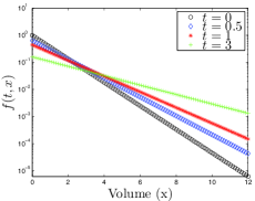
(a) $K_{A}(x,y)\equiv 1$

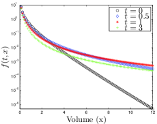
(b) $K_{A}(x,y)=xy$

Figure 2: Analytic solutions - size distribution, $f(t,x)$, vs volume, $x$, for several snapshots in time: $t=0$, $t=0.5$, $t=1$, and $t=3$ in semilog scale. We use $K_{A}(x,y)\equiv 1$ and $K_{A}(x,y)=xy$ as the two aggregation kernels representing a breadth of modeled systems from which we can base comparisons of the two methods studied, the FEM and the FLFM.

4 Computational Results

Using the analytical solutions described in the previous section, we can test both numeric schemes, the FEM and the FLFM, to compare their results. In Section 4.1, we define our measure of error and compare the resulting convergence rates achieved by both methods. In Section 4.2, we compare the FEM’s and the FLFM’s accuracy in approximating the zeroth and first moments. In Section 4.3, we discuss the computation cost required for each of our simulations. Finally, in Section 4.4, we examine the effects of grid spacing and our truncation parameter, $x_{max}$.

4.1 Validation

We cannot overstate the importance of computing the correct norm when determining the error in a particular numerical scheme. In particular, when using the FEM, we approximate $f$, but using the FLFM, we approximate $g$. We then denote the mean analytical solution across the $i^{th}$ element at $t_{k}$ as $f_{i}(t_{k})$ and $g_{i}(t_{k})$ respectively. To compute the error for both methods, we use the grid function norm. For the FEM, we denote the error

$$e_{i}(t_{k})=\left|f_{i}^{N}(t_{k})-\frac{M_{0}(f(t_{k},\cdot);x_{i},x_{i+1})}{\Delta x}\right|=\left|f_{i}^{N}(t_{k})-\pi^{N}(f(t_{k}))\right|$$

and for the FLFM, we denote the error

$$e_{i}(t_{k})=\left|g_{i}^{N}(t_{k})-\frac{M_{1}(\frac{g(t_{k},\cdot)}{\cdot};x_{i},x_{i+1})}{\Delta x}\right|=\left|g_{i}^{N}(t_{k})-g_{i}(t_{k})\right|.$$

In both cases, we generate vectors discretizing an error function, $e(t_{k},x)$, so we calculate the grid function norm as

$$\left\|e(t_{k})\right\|_{1}=\Delta x\sum_{i=1}^{N-1}e_{i}(t_{k}).$$

With our error defined, we aim to reduce the impact of information lost from excluding the interval $[0,x_{1})$ by using the domain $t=[1,3]$. We now compare the accuracy of the two methods for each aggregation kernel, and we plot the results in Figures 3 and 4.

When $K_{A}(x,y)\equiv 1$, the average analytical solution across the $i^{th}$ element is

$$f_{i}(t_{k}) = \frac{1}{\Delta x}\int_{x_{i}}^{x_{i+1}}\left(\frac{2}{2+t}\right)^{2}e^{-\left(\frac{2}{2+t}\right)y}dy$$

$$= \frac{1}{\Delta x}\left(-\frac{2}{2+t}\right)\left[e^{-\frac{2x_{i+1}}{2+t}}-e^{-\frac{2x_{i}}{2+t}}\right],$$

from which we calculate the error in the FEM. Conversely, when we calculate the error in the FLFM, the analytical solution across the $i^{th}$ element is

$$g_{i}(t_{k}) = \frac{1}{\Delta x}\int_{x_{i}}^{x_{i+1}}\left(\frac{2}{2+t}\right)^{2}ye^{-\left(\frac{2}{2+t}\right)y}dy$$

$$= \frac{1}{\Delta x}\left[\left(\frac{2x_{i}}{2+t}+1\right)\left(e^{-\frac{2x_{i}}{2+t}}\right)-\left(\frac{2x_{i+1}}{2+t}+1\right)\left(e^{-\frac{2x_{i+1}}{2+t}}\right)\right].$$

With $K_{A}(x,y)\equiv 1$, $x_{1}$ can be as small as we wish, but physically, $x_{1}>0$, so we choose $x_{1}=10^{-3}$. We should also note that for any choice of $x_{1}>0$, we introduce error by disregarding information generated in the true solution by volumes in the range $[0,x_{1}).$ Under these conditions, we achieve approximately first order accuracy using the finite element approach as depicted in Figure 5. We achieve approximately 1.5 order accuracy using the flux approach, also depicted in Figure 5, and the overall error is much smaller.

When $K_{A}(x,y)=xy$, to calculate error in the FEM approach, we use the average analytical solution across the $i^{th}$ element

$$f_{i}(t_{k})=\frac{1}{\Delta x}\int_{x_{i}}^{x_{i+1}}e^{(-Ty)}\frac{I_{1}(2y\sqrt{t})}{y^{2}\sqrt{t}}dy.$$ (25)

To calculate the error in the FLFM approach, we use the average analytical solution across the $i^{th}$ element

$$g_{i}(t_{k})=\frac{1}{\Delta x}\int_{x_{i}}^{x_{i+1}}e^{(-Ty)}\frac{I_{1}(2y\sqrt{t})}{y\sqrt{t}}dy.$$ (26)

Neither (25) or (26) have analytic integrals, so we apply global adaptive quadrature, as implemented in Matlab’s integral2, with the default relative tolerance of $10^{-6}$ and absolute tolerance of $10^{-10}$, to approximate $f_{i}$ and $g_{i}$ respectively at each time step. Additionally, extremely small volume sizes create large numerical inaccuracies in these integrals, so to achieve the best results, we choose $x_{1}=0.75$. Under these assumptions, we achieve approximately 0.3 order accuracy using the FEM approach, whereas we achieve approximately first order accuracy using FLFM as depicted in Figure 5. For both methods, and with both aggregation kernels, we achieve less accuracy than the maximum achievable by the respective methods, which we address below.

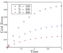
(a) FEM

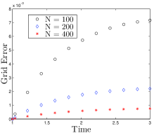
(b) FLFM

Figure 3: Error vs. Time - $L^{1}$ grid error norm vs. time when $K_{A}(x,y)\equiv 1$ for increasing grid densities: $N=100$, $N=200$, and $N=400$ in linear scale. We define the error for the FEM based on the difference between analytic and numeric size distribution, $f$, but we base the error for the FLFM on the difference between analytic and numeric volume distribution, $xf$. The FLFM provides a higher order of accuracy with this aggregation kernel, which represents a system that aggregates slowly and does not experience gelation.

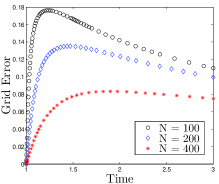
(a) FEM

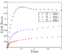
(b) FLFM

Figure 4: Error vs. Time - $L^{1}$ grid error norm vs. time when $K_{A}(x,y)=xy$ for increasing grid densities: $N=100$, $N=200$, and $N=400$ in linear scale. We define the error for the FEM based on the difference between analytic and numeric size distribution, $f$, but we base the error for the FLFM on the difference between analytic and numeric volume distribution, $xf$. The FLFM provides a higher order of accuracy than FEM as well for this aggregation kernel, which represents a rapidly aggregating system where gelation occurs.

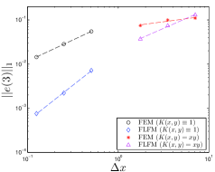
Figure 5: Error vs. $\Delta x$ - $L^{1}$ grid error norm at $t=3$ vs. $\Delta x$ in log scale for both the FEM and the FLFM using both aggregation kernels, $K_{A}(x,y)\equiv 1$ and $K_{A}(x,y)=xy$. The slope of the dashed lines represent the approximate order of accuracy of each method using each respective aggregation kernel. The FEM achieves approximately first and 0.3 order accuracy for the kernels $K_{A}(x,y)\equiv 1$ and $K_{A}(x,y)=xy$ respectively. The FLFM achieves approximately 1.5 and first order for the kernels $K_{A}(x,y)\equiv 1$ and $K_{A}(x,y)=xy$ respectively.

Undoubtedly, the information lost in the interval $[0,x_{1})$ degrades the overall accuracy of the respective methods. In light of these inaccuracies, we offer another test of the methods’ convergence rates for both aggregation kernels. In this second test, we compare solutions for both kernels using 100, 200, 400, 800, and 1600 points to a fine grid solution of 3200 points. The error here is analogous to the error measured when we compare our approximated solutions for varying $N$ to the analytic solution. In the interest of clarity, we use a superscript, *, to denote the error measured when we compare our approximated solutions for varying $N$ to the fine grid solution where $N=3200.$ For the FEM, we then denote the error

$$e_{i}^{*}(t_{k})=\left|f_{i}^{N}(t_{k})-f_{i}^{3200}(t_{k})\right|,$$

and for the FLFM, we denote the error

$$e_{i}^{*}(t_{k})=\left|g_{i}^{N}(t_{k})-g_{i}^{3200}(t_{k})\right|.$$

In both cases, we generate vectors discretizing an error function, $e^{*}(t_{k},x)$, so we calculate the grid function norm as

$$\left\|e^{*}(t_{k})\right\|_{1}=\Delta x\sum_{i=1}^{N-1}e_{i}^{*}(t_{k}).$$

With this test, we achieve an order of accuracy that trends towards second order with each doubling of the number of grid points. These results support our conjecture of second order accuracy for the FEM and support the work in [12] that demonstrates second order accuracy for the FLFM. We depict these results in Figure 6.

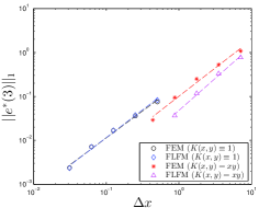
Figure 6: Error vs. $\Delta x$ - $L^{1}$ grid error norm at $t=3$ vs. $\Delta x$ in log scale for both the FEM and the FLFM using the aggregation kernel, $K_{A}(x,y)=xy$. The slope of the dashed lines represents the approximate order of accuracy of each method. Both methods trend towards approximately second order accuracy.

4.2 Moment calculations

In this section, we investigate both methods’ accuracy in approximating the moments. Our study reveals that an inherent advantage of the FEM in its use of a size distribution results in a much more accurate approximation of the zeroth moment when $K_{A}(x,y)\equiv 1$. Conversely, the FLFM’s use of a volume distribution results in a more accurate approximation of the first moment for both aggregation kernels.

Mathematically, we represent total aggregates as the zeroth moment, $M_{0}$, and total volume as the first moment, $M_{1}$, as defined in (1). Different formulations of the governing Smoluchowski equation induce different approaches to calculating the moments numerically. For example, Guy, Fogelson, and Keener [13] extend the generating function approach described in [39] to study blood clots. In the FEM approach, we approximate the size distribution across the $i^{th}$ element as $f_{i}^{N}(t_{k})$, whereas with the FLFM, we approximate the volume distribution across the $i^{th}$ element as $g_{i}^{N}(t_{k})$. Using (1) with our known analytical solutions for $f(t,x)$, the analytical total number of particles in our truncated system is

$$M_{0}(t_{k})=\int_{x_{1}}^{x_{N}}f(t_{k},y)dy=\int_{x_{1}}^{x_{N}}\frac{g(t_{k},y)}{y}dy,$$ (27)

and the analytical total volume in our truncated system is

$$M_{1}(t_{k})=\int_{x_{1}}^{x_{N}}yf(t_{k},y)dy=\int_{x_{1}}^{x_{N}}g(t_{k},y)dy.$$ (28)

We acknowledge the mild abuse of the notation in redefining $M_{i}$ in (27) and (28) in the name of focusing attention on how the moment changes as a function of time. In what follows we will clearly note when referring to moments of the FEM or the FLFM solutions. We demonstrate below that the FEM more accurately approximates the zeroth moment when $K_{A}(x,y)\equiv 1$.

Through contrasting our approximations of the zeroth moment by the two methods studied in this paper, we derive an important advantage that the FEM possesses at $t=0$ for a slowly aggregating system (e.g., $K_{A}(x,y)\equiv 1$). In this case, for the FEM,

$$M_{0}^{N}(t_{k})=\sum_{i=1}^{N-1}\int_{x_{i}}^{x_{i+1}}e^{-y}dy=M_{0}(0),$$

but for the FLFM

$$M_{0}^{N}(0)=\sum_{i=1}^{N-1}\left[\left(\frac{1}{\Delta x}\left\{\left(x_{i}+1\right)e^{-x_{i}}-\left(x_{i+1}+1\right)e^{-x_{i+1}}\right\}\right)\ln\left(\frac{x_{i+1}}{x_{i}}\right)\right]\approx M_{0}(0).$$

To derive this result, we start with the general formulation of the zeroth moment at $t_{k}$. For the FEM,

$$M_{0}^{N}(t_{k})=\int_{x_{1}}^{x_{N}}f_{i}^{N}(t_{k})dy=\Delta x\sum_{i=1}^{N-1}f_{i}^{N}(t_{k}),$$

whereas with the FLFM

$$M_{0}^{N}(t_{k})=\int_{x_{1}}^{x_{N}}\frac{g_{i}^{N}(t_{k})}{y}dy=\sum_{i=1}^{N-1}\left[g_{i}^{N}(t_{k})\ln\left(\frac{x_{i+1}}{x_{i}}\right)\right].$$

Then at $t=0$ and with $K_{A}(x,y)\equiv 1$, we have $f(0,x)=e^{-x}$ and $g(0,x)=xe^{-x}$, which we initialize numerically via (7) and (22) respectively. The analytical zeroth moment,

$$M_{0}(0)=\int_{x_{1}}^{x_{N}}f(0,y)dy=\sum_{i=1}^{N-1}\int_{x_{i}}^{x_{i+1}}e^{-y}dy,$$

matches the approximation by the FEM,

$$M_{0}^{N}(0)=\int_{x_{1}}^{x_{N}}f_{i}^{N}(0)dy=\Delta x\sum_{i=1}^{N-1}f_{i}^{N}(0)=\sum_{i=1}^{N-1}\int_{x_{i}}^{x_{i+1}}e^{-y}dy.$$

Conversely, the approximation by the FLFM,

$$M_{0}^{N}(0) = \int_{x_{1}}^{x_{N}}\frac{g_{i}^{N}(0)}{y}dy=\sum_{i=1}^{N-1}\left[g_{i}^{N}(0)\ln\left(\frac{x_{i+1}}{x_{i}}\right)\right]$$

$$= \sum_{i=1}^{N-1}\left[\left(\frac{1}{\Delta x}\left\{\left(x_{i}+1\right)e^{-x_{i}}-\left(x_{i+1}+1\right)e^{-x_{i+1}}\right\}\right)\ln\left(\frac{x_{i+1}}{x_{i}}\right)\right],$$

is clearly not the same as $M_{0}(0)$. Not surprisingly, our outputs for $M_{0}^{N}(0)$ vary slightly in Figure 7a such that $M_{0}^{N}(0)=M_{0}(0)\approx 0.999$ using the FEM, but $M_{0}^{N}(0)\approx 1.169$ using the FLFM. Along similar lines, when $K_{A}(x,y)=xy$, we have $M_{0}(0)$ matching the approximation by the FEM where $M_{0}^{N}(0)\approx 0.34$, but the FLFM produces $M_{0}^{N}(0)\approx 0.2916$ as depicted in Figure 7b. We summarize these results in Table 1. Clearly, with experimental data in the form of a size distribution, the FLFM starts at a disadvantage approximating the zeroth moment since its approximation at $t=0$ contains error. Furthermore, the FEM maintains a better approximation of the zeroth moment as depicted in Figure 8a.

Now contrasting our approximations of the first moment, we demonstrate more accuracy by the FLFM than by the FEM. Using the FEM,

$$M_{1}^{N}(t_{k})=\int_{x_{1}}^{x_{N}}yf(t_{k},y)dy\approx\frac{1}{2}\sum_{i=1}^{N-1}f_{i}^{N}(t_{k})(x_{i+1}^{2}-x_{i}^{2}),$$

whereas using the FLFM,

$$M_{1}^{N}(t_{k})\approx\int_{x_{1}}^{x_{N}}g_{i}^{N}(t_{k})dy=\Delta x\sum_{i=1}^{N-1}g_{i}^{N}(t_{k}).$$

In this case, with $t=0$ and $K_{A}(x,y)\equiv 1$, $M_{1}^{N}(0)=M_{1}(0)\approx 1.0000$ using the FLFM, but $M_{1}^{N}(0)\approx 1.0013$ using the FEM. Similarly, when $t=0$ and $K_{A}(x,y)=xy$, $M_{1}(0)$ matches the approximation using the FLFM where $M_{1}^{N}(0)\approx 0.472$, but the FEM produces $M_{1}^{N}(0)\approx 0.602$. We summarize these results in Table 1.

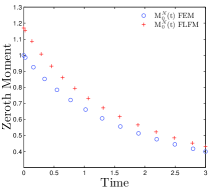
(a) $K_{A}(x,y)\equiv 1$

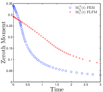
(b) $K_{A}(x,y)=xy$

Figure 7: $M_{0}^{400}(t)$ vs. Time - Numerical approximation of the zeroth moment for a truncated volume domain, $x_{1}$ to $x_{400}$, for both aggregation kernels. Note, with the FEM, $M_{0}^{400}(0)=M_{0}(0),$ but with the FLFM, $M_{0}^{400}(0)\approx M_{0}(0)$. When given data in the form of a size distribution, the FEM’s approximation of the total particles in a system starts with an advantage over the FLFM’s approximation, which has error at $t=0$. We use a linear scale for both plots.

	Analytical	FEM	FLFM
$M_{0}(0)$	0.999	0.999	1.169
$M_{1}(0)$	1.0000	1.0013	1.0000

(a) $K_{A}(x,y)\equiv 1$

	Analytical	FEM	FLFM
$M_{0}(0)$	0.34	0.34	0.2916
$M_{1}(0)$	0.472	0.602	0.472

(b) $K_{A}(x,y)=xy$

Table 1: Comparison of analytical partial $i^{th}$ moments ($i=0,1$) at $t=0$ with the approximations by both the FEM and the FLFM. The analytical $M_{0}(0)$ exactly matches that of the FEM, but the FLFM’s approximation of $M_{0}(0)$ contains error. Conversely, the analytical $M_{1}(0)$ exactly matches that of the FLFM, but the FEM’s approximation of $M_{1}(0)$ contains error.

Having illuminated the respective advantages the FEM has approximating the zeroth moment, and the FLFM has approximating the first moment, we now examine the convergence rates of the two methods to a fine grid ($N=3200$) approximation of the moments. In this case, we compute the difference between the lower resolution grid ($N=100,\,200,\,400,\,800,\,1600)$ approximations of the moments at $t=3$, and the fine grid ($N=3200$) approximation. We denote the difference in the approximations of the zeroth moment, $M_{0}^{diff}$, and the difference in the approximations of the first moment, $M_{1}^{diff}$ where

$$M_{0}^{diff} = \left|M_{0}^{N}(3)-M_{0}^{3200}(3)\right|$$

$$M_{1}^{diff} = \left|M_{1}^{N}(3)-M_{1}^{3200}(3)\right|.$$

Our simulations include both aggregation kernels, and we depict the convergence rates in Figures 8a and 8b. As expected, for both methods, we observe a trend towards second order accuracy (more evidence supporting our claim of second order convergence for the FEM). Intriguingly, when $K_{A}(x,y)\equiv 1$, the FEM more accurately predicts the zeroth moment. In this case, given experimental data in the form of a size distribution and a system experiencing slow aggregation, the FEM is a better choice of methods. We summarize convergence rates of these simulations in Table 2, and note that as the number of grid points double the convergence rates tend toward the expected convergence rates described in Sections 2.2 and 2.3.

	Method	Moment	100$\rightarrow$200	200$\rightarrow$400	400$\rightarrow$800	800$\rightarrow$1600
$K\equiv 1$	FEM	Zeroth	0.2	1.1	1.2	1.4
		First	1.1	1.1	1.2	1.6
	FLFM	Zeroth	1.2	1.3	1.5	1.8
		First	0.6	1.4	1.7	2
$K=xy$	FEM	Zeroth	0.2	0.5	1.3	1.6
		First	0.5	1.0	1.0	1.5
	FLFM	Zeroth	0.7	1.5	1.4	*4
		First	1.4	6.6	*	*4

Table 2: Convergence rates of coarse grid ($N=100,\,200,\,400,\,800,\,1600)$ approximations of the zeroth and first moments to a fine grid ($N=3200$) approximation of the moments. In all cases, we observe a trend towards second order convergence.

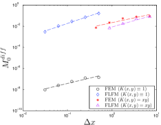
(a) Zeroth Moment

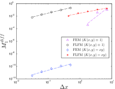
(b) First Moment

Figure 8: Moment differences at $t=3$ vs. $\Delta x$ - Difference between approximations of the zeroth and first moments by coarse grid ($N=100,\,200,\,400,\,800,\,1600$) simulations and the approximation by the fine grid ($N=3200$) simulation. In all cases, we observe a trend towards second order convergence, with one case (slow aggregation, e.g., $K_{A}(x,y)\equiv 1$ and zeroth moment approximation) where the FEM is more accurate.

4.3 Computation cost

Clearly, order of accuracy is important, but we also want to know which method requires more computation in terms of floating point operations. To make the comparisons, we compute the floating point operations for the simulations discussed in Section 4.1 for both the FEM and the FLFM. The number of operations counted includes only the computations required for each algorithm to solve the system of ODEs at a given point in time, $t_{k}$. We implement the simulations using Matlab version 2013a on an Intel(R) Core(TM) i-5 2410M CPU @ 2.3 GHz. For each simulation, the FEM requires significantly less floating point operations than the FLFM. The results are summarized in Table 3 and give us important insights. When $K_{A}(x,y)\equiv 1$, the required number of floating point operations and an extrapolation of the error data in Figure 5 imply that the FEM with 800 grid points can achieve nearly equal accuracy as the FLFM with 100 grid points. The FEM achieves this accuracy with only 38% of the floating point operations that it takes the FLFM, so when computation cost is more valuable to the user, the FEM provides a better choice.

		$N=100$	$N=200$	$N=400$	$N=800$
$K(x,y)\equiv 1$	FEM	$1.46\times 10^{4}$	$5.93\times 10^{4}$	$2.39\times 10^{5}$	$9.57\times 10^{5}$
	FLFM	$2.49\times 10^{6}$	$1.99\times 10^{7}$	$1.60\times 10^{8}$	$1.28\times 10^{9}$
$K(x,y)=xy$	FEM	$6.71\times 10^{4}$	$2.74\times 10^{5}$	$1.11\times 10^{6}$	$4.46\times 10^{6}$
	FLFM	$2.48\times 10^{6}$	$1.99\times 10^{7}$	$1.60\times 10^{8}$	$1.28\times 10^{9}$

Table 3: Comparison of floating point operations required to solve the right hand side system of ODEs for any $t_{k}$ for both the FEM and the FLFM. We perform the simulations on a 2.3 GHz processor. When $K(x,y)\equiv 1$, the number of floating point operations performed for the FEM simulation with 800 grid points requires only 38% of the number of floating point operations that the FLFM simulation with 100 grid points requires. The error is nearly the same for both simulations implying that if computation cost is more valuable to the user, the FEM should be the choice of methods.

4.4 Relationship between $x_{max}$ and $\Delta x$

In [12], Filbet and Laurençot report sensitivity of the FLFM to the truncation parameter, $x_{max}.$ We study the error as a function of both $x_{max}$ and $\Delta x$, and in particular, we would like determine to what extent the truncation parameter, $x_{max}$, impacts the overall accuracy of the two schemes. We do not find the following results conclusive, but they do reveal intriguing patterns that we plan to study more extensively in future work.

Note that for each run and a given value of $x_{max}$, we initialize our grid with $x_{1}=0.001$ when $K_{A}(x,y)\equiv 1$ and with $x_{1}=0.75$ when $K_{A}(x,y)=xy$. Notice in Figures 9 and 10, for a given $\Delta x$, using both the FEM and the FLFM, the error is the same regardless of the value of $x_{max}$ for both kernels, and we achieve the expected behavior of decreasing error with refinement of the grid. We suggest that when $K_{A}(x,y)\equiv 1$ with the initial conditions used in this study, the analytic solutions decay so quickly that the numeric approximations do not suffer greatly from the truncation parameter, $x_{max}$, for either method as evidenced in Figure 9. However, when $K_{A}(x,y)=xy$, we cannot make the same general statement. Using the FLFM with $x_{max}=80$, $x_{max}=160$, and $x_{max}=320$, we actually achieve reduced error for larger grid spacing as depicted in Figure 10b, which is consistent with the poor results noted by Filbet and Laurençot in [12]. Practically speaking, if we wanted to model a system experiencing rapid aggregation and faced limits on gathering data for aggregates with large volume, the FEM would provide more accurate results.

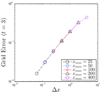
(a) FEM

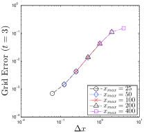
(b) FLFM

Figure 9: Error vs $\Delta x$ - Grid error at $t=3$ vs. uniform grid spacing, $\Delta x$, when $K_{A}(x,y)\equiv 1$, for $x_{max}=25,$ $x_{max}=50,$ $x_{max}=100$, $x_{max}=200$, and $x_{max}=400$ in log scale. Clearly, with a slowly aggregating system, grid spacing plays the primary role in accuracy for both methods studied in the paper.

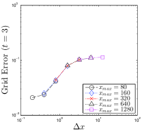
(a) FEM

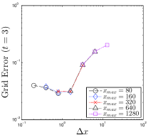
(b) FLFM

Figure 10: Error vs $\Delta x$ - Grid error at $t=3$ vs. uniform grid spacing, $\Delta x$, when $K_{A}(x,y)=xy$, for $x_{max}=80,$ $x_{max}=160,$ $x_{max}=320$, $x_{max}=640$, and $x_{max}=1280$ in log scale. For the FEM, grid spacing plays a more important role in accuracy than the truncation parameter, $x_{max}$, but the FLFM experiences poor behavior when $x_{max}$ is too small.

5 Conclusions and Future Work

The Smoluchowski coagulation equation provides a useful model of particles in suspension in diverse fields of study. Because only a few analytical solutions exist, researchers have developed numerical approaches to approximate solutions to the model. With an eventual goal of comparing simulated solutions with experimental data, we compare two method’s accuracies in approximating known and fine grid solutions as well as their accuracies in approximating the zeroth and first moments. We also compare the computation cost of the two methods.

In [2], Ackleh and Fitzpatrick report first order convergence of the FEM in $L^{\infty}[\boldsymbol{X}]$, and in [12], Filbet and Laurençot, report second order convergence of the FLFM in $L^{1}[\boldsymbol{X}]$. Our results support (our conjecture) of second order convergence of the FEM in $L^{1}[\boldsymbol{X}]$ and second order convergence of the FLFM in $L^{1}[\boldsymbol{X}]$, which eliminates any speed advantage the FLFM was previously understood to possess. Furthermore, when approximating a fine grid solution the two methods achieve nearly equal accuracy, with the FLFM achieving slightly higher accuracy for the multiplicative kernel.

Experimental data comes in different forms such as partial zeroth moment distributions or partial first moment distributions. We also theoretically consider the moment approximations and provide numerical evidence that .the FLFM is slightly more accurate approximating the zeroth moment for quickly aggregating systems, and the FEM is much more accurate approximating the zeroth moment when the system aggregates slowly. In terms of approximating the first moment, the FLFM is more accurate for both quickly and slowly aggregating systems.

We also identified discretization resolutions where for the same level of accuracy, the FEM exhibits substantial savings in computational cost over the FLFM For example, the FEM on 800 grid points offers an opportunity of computation cost savings over using the FLFM on 100 grid points while achieving nearly equal accuracy.

We also study the error as a function of both $x_{max}$ and $\Delta x$ in an effort to determine the extent to which the truncation parameter, $x_{max}$, impacts the overall accuracy of the two schemes. Our initial results suggest two important results. The first is not surprising: in general, for the aggregation kernels in this study, reduced grid spacing plays the predominant role in improving numerical accuracy. Second, the FLFM suffers from sensitivity to truncation parameter, $x_{max},$ when $K_{A}(x,y)=xy,$ so if experimental data includes a small $x_{max}$, the FEM should be the method of choice. These intriguing patterns will motivate a more extensive theoretical study of these issue in the future.

6 Acknowledgements

This work was supported in part by the National Science Foundation grant DMS-1225878.

Appendix A Example Calculation of Flux Derivative for FLFM

To illustrate how we calculate the right hand side of our second order spatial approximation in (21), we offer the following example set of calculations. At a given time step, $k$, consider $J_{3}^{N}(t_{k}).$ We have fixed $r=3$, and then we fix $x_{mid(1)}$, therefore on a uniform grid, $\tilde{x}\geq x_{3}-x_{mid(1)}=x_{mid(2)}$. We now know that $x_{mid(1)}+x_{mid(j)}\geq x_{3}\,\mbox{for}\,j\in[2,N]$, so the contribution to $J_{3}^{N}(t_{k})$ by aggregates in the first element is

$$\Delta xg_{1}^{N}(t_{k})\left[\int_{x_{mid(2)}}^{x_{3}}\frac{K_{A}(x_{mid(1)},y)}{y}g_{2}^{N}(t_{k})dy+\sum_{j=3}^{N-1}\left(\int_{x_{j}}^{x_{j+1}}\frac{K_{A}(x_{mid(1)},y)}{y}g_{j}^{N}(t_{k})dy\right)\right].$$

We then consider contributions of aggregates with volume $x_{mid(2)}$, which leads to $\tilde{x}\geq x_{3}-x_{mid(2)}=x_{mid(1)}$. This implies $j\in[1,N]$ for contributions to $J_{3}^{N}(t_{k})$ by aggregates in the second element amounting to

$$\Delta xg_{2}^{N}(t_{k})\left[\int_{x_{mid(1)}}^{x_{2}}\frac{K_{A}(x_{mid(1)},y)}{y}g_{1}^{N}(t_{k})dy+\sum_{j=2}^{N-1}\left(\int_{x_{j}}^{x_{j+1}}\frac{K_{A}(x_{mid(1)},y)}{y}g_{j}^{N}(t_{k})dy\right)\right].$$

We now have our total flux across $x_{3}$

$$J_{3}^{N}(t_{k}) = \Delta xg_{1}^{N}(t_{k})\left[\int_{x_{mid(2)}}^{x_{3}}\frac{K_{A}(x_{mid(1)},y)}{y}g_{2}^{N}(t_{k})dy+\sum_{j=3}^{N-1}\left(\int_{x_{j}}^{x_{j+1}}\frac{K_{A}(x_{mid(1)},y)}{y}g_{j}^{N}(t_{k})dy\right)\right]$$

$$+ \Delta xg_{2}^{N}(t_{k})\left[\int_{x_{mid(1)}}^{x_{2}}\frac{K_{A}(x_{mid(1)},y)}{y}g_{1}^{N}(t_{k})dy+\sum_{j=2}^{N-1}\left(\int_{x_{j}}^{x_{j+1}}\frac{K_{A}(x_{mid(1)},y)}{y}g_{j}^{N}(t_{k})dy\right)\right].$$

At this point, we can generalize the flux at any given element boundary ($i\in[2,N]$) as

$$J_{i}^{N}(t_{k})=\sum_{p=1}^{i-1}\Delta xg_{p}^{N}(t_{k})\left\{\int_{x_{mid(i-p)}}^{x_{i-p+1}}\frac{K_{A}(x_{mid(p)},y)}{y}dy\,g_{i-p}^{N}(t_{k})+\sum_{j=i-p+1}^{N-1}\int_{x_{j}}^{x_{j+1}}\frac{K_{A}(x_{mid(p)},y)}{y}dy\,g_{j}^{N}(t_{k})\right\}.$$ (29)

Specifically, when $K_{A}(x,y)\equiv 1$,

$$J_{i}^{N}(t_{k})=\sum_{p=1}^{i-1}\Delta xg_{p}^{N}(t_{k})\left\{\int_{x_{mid(i-p)}}^{x_{i-p+1}}\frac{1}{y}dy\,g_{i-p}^{N}(t_{k})+\sum_{j=i-p+1}^{N-1}\int_{x_{j}}^{x_{j+1}}\frac{1}{y}dy\,g_{j}^{N}(t_{k})\right\},$$

which after integration gives us

$$J_{i}^{N}(t_{k})=\sum_{p=1}^{i-1}\Delta xg_{p}^{N}(t_{k})\left\{\ln\frac{x_{i-p+1}}{x_{mid(i-p)}}\,g_{i-p}^{N}(t_{k})+\sum_{j=i-p+1}^{N-1}\ln\frac{x_{j+1}}{x_{j}}\,g_{j}^{N}(t_{k})\right\},$$

and when $K_{A}(x,y)=xy$,

$$J_{i}^{N}(t_{k})=\sum_{p=1}^{i-1}\Delta xg_{p}^{N}(t_{k})\left\{\int_{x_{mid(i-p)}}^{x_{i-p+1}}\frac{x_{mid(p)}y}{y}dy\,g_{i-p}^{N}(t_{k})+\sum_{j=i-p+1}^{N-1}\int_{x_{j}}^{x_{j+1}}\frac{x_{mid(p)}y}{y}dy\,g_{j}^{N}(t_{k})\right\},$$

which after integration gives us

$$J_{i}^{N}(t_{k})=\sum_{p=1}^{i-1}\Delta xg_{p}^{N}(t_{k})\left\{.5\Delta x\cdot x_{mid(p)}\,g_{i-p}^{N}(t_{k})+\sum_{j=i-p+1}^{N-1}x_{mid(p)}\Delta x\,g_{j}^{N}(t_{k})\right\}.$$

Appendix B Solution at $t=0$ for $K_{A}(x,y)=xy$

For the analytical solution used in the paper when $K_{A}(x,y)=xy$, note that $f(0,x)=\frac{e^{-x}}{x}$, which is not necessarily obvious. The derivation of those initial conditions follow. From (24),

$$f(t,x)=e^{(-Tx)}\frac{I_{1}(2x\sqrt{t})}{x^{2}\sqrt{t}},$$ (30)

where

$$T=\left\{\begin{array}[]{ll}1+t&\mbox{if}\,\,t\leq 1\\ 2\sqrt{t}&\mbox{otherwise}\end{array}\right.,$$

and we use the modified Bessel function of the first kind

$$I_{1}(x)=\frac{1}{\pi}\int_{0}^{\pi}e^{x\,\cos\theta}\cos\theta d\theta.$$

For this solution, $f(0,x)=\frac{e^{-x}}{x}$. Note that for $t\leq 1$,

$$f(t,x)=\frac{e^{(-x-tx)}I_{1}(2x\sqrt{t})}{x^{2}\sqrt{t}}$$

with

$$I_{1}(2x\sqrt{t})=\frac{1}{\pi}\int_{0}^{\pi}e^{(2x\sqrt{t}\cos\theta)}\cos\theta d\theta.$$

Now note the following:

1. $\lim_{t\rightarrow 0}\frac{I_{1}(2x\sqrt{t})}{x^{2}\sqrt{t}}=\lim_{t\rightarrow 0}\frac{1}{\pi}\int_{0}^{\pi}\frac{e^{(2x\sqrt{t}cos\theta)}\cos\theta}{x^{2}\sqrt{t}}d\theta$

2. e${}^{(2x\sqrt{t}\cos\theta)}=1+(2x\sqrt{t}\cos\theta)+\frac{(2x\sqrt{t}\cos\theta)^{2}}{2!}+\cdots$

therefore,

$$\lim_{t\rightarrow 0}\frac{I_{1}(2x\sqrt{t})}{x^{2}\sqrt{t}} = \lim_{t\rightarrow 0}\frac{1}{\pi}\int_{0}^{\pi}\frac{\cos\theta+2x\sqrt{t}\cos^{2}\theta}{x^{2}\sqrt{t}}d\theta+\frac{1}{\pi}\int_{0}^{\pi}\lim_{t\rightarrow 0}\left[\frac{(2x\sqrt{t}\cos\theta)^{2}\cos\theta}{2!x^{2}\sqrt{t}}+\cdots\right]d\theta$$

$$= \lim_{t\rightarrow 0}\frac{1}{\pi}\int_{0}^{\pi}\frac{\cos\theta}{x^{2}\sqrt{t}}d\theta+\lim_{t\rightarrow 0}\frac{1}{\pi}\int_{0}^{\pi}\frac{2\cos^{2}\theta}{x}d\theta+0$$

$$= 0+\lim_{t\rightarrow 0}\frac{2}{\pi x}(\frac{\pi}{2})=\frac{1}{x}$$

from which it follows that

$$\lim_{t\rightarrow 0}f(t,x)=\left[\lim_{t\rightarrow 0}e^{(-x-tx)}\right]\left[\lim_{t\rightarrow 0}\frac{I_{1}(2x\sqrt{t})}{x^{2}\sqrt{t}}\right]=\frac{e^{-x}}{x}.$$

References

• [1] A. S. Ackleh. Parameter estimation in a structured algal coagulation-fragmentation model. Nonlinear Anal., 28(5):837–854, Mar. 1997.
• [2] A. S. Ackleh and B. G. Fitzpatrick. Modeling aggregation and growth processes in an algal population model: analysis and computations. J. Math. Biol., 35(4):480–502, Mar. 1997.
• [3] D. J. Aldous. Deterministic and Stochastic Models for Coalescence (Aggregation, Coagulation): A Review of the Mean-Field Theory for Probabilists. Bernoulli, 5(1):3–48, 1999.
• [4] T. A. Bak and O. Heilmann. A finite version of Smoluchowski’s coagulation equation. J. Phys. A. Math. Gen., 24(20):4889–4893, Oct. 1991.
• [5] H. T. Banks and F. Kappel. Transformation semigroups andL 1-approximation for size structured population models. Semigr. Forum, 38(1):141–155, Dec. 1989.
• [6] J. C. Barrett and J. S. Jheeta. Improving the accuracy of the moments method for solving the aerosol general dynamic equation. J. Aerosol Sci., 27(8):1135–1142, Dec. 1996.
• [7] B. J. Berne and R. Pecora. Dynamic Light Scattering: With Applications to Chemistry, Biology, and Physics. Courier Dover Publications, 2000.
• [8] D. M. Bortz, T. L. Jackson, K. A. Taylor, A. P. Thompson, and J. G. Younger. Klebsiella pneumoniae flocculation dynamics. Bull. Math. Biol., 70(3):745–68, Apr. 2008.
• [9] F. P. da Costa. A Finite-Dimensional Dynamical Model for Gelation in Coagulation Processes. J. Nonlinear Sci., 8(6):619–653, Dec. 1998.
• [10] R. L. Drake. A General Mathematical Survey of the Coagulation Equation. In G. M. Hidy and J. R. Brock, editors, Top. Curr. Aerosol Res. (Part 2), volume 3 of International Reviews in Aerosol Physics and Chemistry, pages 201–376. Pergamon Press, New York, NY, 1972.
• [11] M. H. Ernst, R. M. Ziff, and E. M. Hendriks. Coagulation processes with a phase transition. J. Colloid Interface Sci., 97(1):266–277, Jan. 1984.
• [12] F. Filbet and P. Laurençot. Numerical Simulation of the Smoluchowski Coagulation Equation. SIAM J. Sci. Comput., 25(6):2004, 2004.
• [13] R. D. Guy, A. L. Fogelson, and J. P. Keener. Fibrin gel formation in a shear flow. Math. Med. Biol., 24(1):111–130, 2007.
• [14] T. Kiørboe. Formation and fate of marine snow: small-scale processes with large-scale implications. Sci. Mar., 65:57–71, 2001.
• [15] F. E. Kruis, A. Maisels, and H. Fissan. Direct simulation Monte Carlo method for particle coagulation and aggregation. AIChE J., 46(9):1735–1742, Sept. 2000.
• [16] J. Kumar, G. Warnecke, M. Peglow, and S. Heinrich. Comparison of numerical methods for solving population balance equations incorporating aggregation and breakage. Powder Technol., 189(2):218–229, Jan. 2009.
• [17] M. H. Lee. On the Validity of the Coagulation Equation and the Nature of Runaway Growth. Icarus, 143(1):74–86, Jan. 2000.
• [18] M. H. Lee. A survey of numerical solutions to the coagulation equation. J. Phys. A. Math. Gen., 34(47):10219–10241, Nov. 2001.
• [19] R. J. LeVeque. Finite Difference Methods for Ordinary and Partial Differential Equations: Steady-State and Time-Dependent Problems. SIAM, Philadelphia, PA, 2007.
• [20] Y. Lin, K. Lee, and T. Matsoukas. Solution of the population balance equation using constant-number Monte Carlo. Chem. Eng. Sci., 57:2241–2252, 2002.
• [21] G. Madras and B. J. McCoy. Reversible crystal growth dissolution and aggregation breakage: numerical and moment solutions for population balance equations. Powder Technol., 143-144:297–307, June 2004.
• [22] A. W. Mahoney and D. Ramkrishna. Efficient solution of population balance equations with discontinuities by finite elements. Chem. Eng. Sci., 57:1107–1119, 2002.
• [23] J. Makino, T. Fukushige, Y. Funato, and E. Kokubo. On the mass distribution of planetesimals in the early runaway stage. New Astron., 3:411–417, 1998.
• [24] H. Müller. Zur allgemeinen Theorie der raschen Koagulation. Kolloidchem. Beihefte, 27:257–311, 1928.
• [25] H.-S. Niwa. School size statistics of fish. J. Theor. Biol., 195(3):351–61, Dec. 1998.
• [26] H. R. Pruppacher and J. D. Klett. Microphysics of Clouds and Precipitation. Riedel, Boston, MA, 1980.
• [27] D. Ramkrishna. Population Balances: Theory and Applications to Particulate Systems in Engineering. Academic Press, San Diego, CA, 2000.
• [28] M. Ranjbar, H. Adibi, and M. Lakestani. Numerical solution of homogeneous Smoluchowski’s coagulation equation. Int. J. Comput. Math., 87(9):2113–2122, July 2010.
• [29] U. Riebesell and D. A. Wolf-Gladrow. The relationship between physical aggregation of phytoplankton and particle flux: A numerical model. Deep. Res., 39(7/8):1085–1102, 1992.
• [30] H. M. Shapiro. Practical Flow Cytometry. John Wiley and Sons, 2005.
• [31] J. Silk and S. D. White. The development of structure in the expanding universe. Astrophys. J., 1978.
• [32] M. P. Surh, J. B. Sturgeon, and W. G. Wolfer. Void nucleation, growth, and coalescence in irradiated metals. J. Nucl. Mater., 378(1):86–97, Aug. 2008.
• [33] M. van Smoluchowski. Drei Vorträge über Diffusion, Brownsche Bewegung und Koagulation von Kolloidteilchen. Zeitschrift für Phys., 17:557–571, 1916.
• [34] M. van Smoluchowski. Versuch einer mathematischen theorie der koagulation kinetic kolloider losungen. Zeitschrift für Phys. Chemie, 92:129–168, 1917.
• [35] D. Verkoeijen, G. A. Pouw, G. M. H. Meesters, and B. Scarlett. Population balances for particulate processes a volume approach. Chem. Eng. Sci., 57(12):2287–2303, June 2002.
• [36] J. A. D. Wattis. An introduction to mathematical models of coagulation-fragmentation processes: A discrete deterministic mean-field approach. Phys. D Nonlinear Phenom., 222(1-2):1–20, Oct. 2006.
• [37] Y. Yang and C.-W. Shu. Analysis of optimal superconvergence of discontinuous Galerkin method for linear hyperbolic equations. SIAM J. Numer. Anal., 50(6):3110–3133, Jan. 2012.
• [38] J. Zhe, A. Jagtiani, P. Dutta, J. Hu, and J. Carletta. A micromachined high throughput Coulter counter for bioparticle detection and counting. J. Micromechanics Microengineering, 17(2):304–313, Feb. 2007.
• [39] R. M. Ziff and G. Stell. Kinetics of polymer gelation. J. Chem. Phys., 73(7):3492, 1980.