Sub-Classifier Construction for Error Correcting Output Code Using Minimum Weight Perfect Matching

Abstract

Multi-class classification is mandatory for real world problems and one of promising techniques for multi-class classification is Error Correcting Output Code. We propose a method for constructing the Error Correcting Output Code to obtain the suitable combination of positive and negative classes encoded to represent binary classifiers. The minimum weight perfect matching algorithm is applied to find the optimal pairs of subset of classes by using the generalization performance as a weighting criterion. Based on our method, each subset of classes with positive and negative labels is appropriately combined for learning the binary classifiers. Experimental results show that our technique gives significantly higher performance compared to traditional methods including the dense random code and the sparse random code both in terms of accuracy and classification times. Moreover, our method requires significantly smaller number of binary classifiers while maintaining accuracy compared to the One-Versus-One.

I Introduction

Error Correcting Output Code (ECOC) [1, 2] is one of the well-known techniques for solving multiclass classification. Based on this framework, an unknown-class instance will be classified by all binary classifiers corresponding to designed columns of the code matrix, and then the class with the closet codeword is assigned to the final output class. Each individual binary function including the large number of classes indicates the high capability as a shared classifier. Generally, when the number of classes increases, the complexity for creating the hyperplane also increases. The suitable combination of classes with the proper number of classes for constructing the model is still a challenge issue to obtain the effective classifier.

Several classic works are applied to the design of the code matrix such as One-Versus-One (OVO) [3], One-Versus-All (OVA) [4], dense random code, and sparse random code [1, 2], and for an $N$ class problem, they provide the number of binary models of $N(N-1)/2$, $N$, $\lceil 10log_{2}N\rceil$, and $\lceil 15log_{2}N\rceil$, respectively. Moreover, some approaches using the genetic algorithm have been proposed [5, 6]. However, according to the complexity of the problem that the solutions are searched from a large space including all possible $2^{N-1}-1$ columns [1] in case of dense code, and $\frac{3^{N}-2^{N+1}+1}{2}$ columns [7] in case of sparse code, design of code matrix is still ongoing research.

This research aims to find the suitable combination of classes for creating the binary models in the ECOC framework by providing both good classification accuracy and the small number of classifiers. Our method is based on the minimum weight perfect matching algorithm by using the relation between pair of subset of classes defined by the generalization performance as the criterion for constructing the code matrix. We study this multiclass classification based on Support Vector Machines [8, 9] as base learners. We also empirically evaluate our technique by comparing with the traditional methods on ten datasets from the UCI Machine Learning Repository [10].

This paper is organized as follows. Section II reviews the traditional ECOC frameworks. Section III presents our proposed method. Section IV performs experiments and explains the results and discussions. Section V concludes the research and directions for the future work.

II Error Correcting Output Codes

Error Correcting Output Code (ECOC) was introduced by Dietterich and Bakiri [1] as a combining framework for multiclass classification. For a given code matrix with $N$ rows and $L$ columns, each element contains either $\textquoteleft$1’, or $\textquoteleft$-1’. This code matrix is designed to represent a set of $L$ binary learning problems for $N$ classes. Each specific class is defined by the unique bit string called codeword and each sub-problem is indicated by the combination of positive and negative classes corresponding to the elements of the code matrix. Moreover, in order to allow the binary model learned without considering some particular classes, Allwein et al. [2] extended the coding method by adding the third symbol $\textquoteleft$0’ as “ don’t care bit”. Unlike the previous method, the number of classes for training a binary classifier can be varied from 2 to $N$ classes.

Several classic coding designs have been proposed, e.g., One-Versus-All (OVA) [4], dense random codes, sparse random codes [2], and One-Versus-One (OVO) [3]; the first two techniques and the last two techniques are binary and ternary strategies, respectively. One-Versus-All codes including $N$ columns were designed by setting the $i^{th}$ class, and the remaining classes labeled with the positive and negative classes, respectively. Dense random codes and sparse random were introduced by randomizing sets of $\lceil 10log_{2}N\rceil$ and $\lceil 15log_{2}N\rceil$ binary functions, respectively. In case of One-Versus-One codes, they were designed to define each column by labeling $\textquoteleft$1’ and $\textquoteleft$-1’ to only two out of $N$ classes, and therefore there are $N(N-1)/2$ possible columns.

For a decoding process, an instance with unknown-class will be classified by all $L$ binary functions corresponding to designed columns of the code matrix. This output vector is compared to each row of the code matrix. The class corresponding the row of code matrix that provides highest similarity is assigned as the final output class. Several similarity measures have been proposed such as Hamming distance [1], Euclidean distance [11], extended strategies based on these two methods  [11], and the loss-based technique [2].

III Proposed Method

We aim to construct the code matrix in which each column is a suitable combination of positive and negative classes encoded to represent a binary model. As mentioned before, the best code matrix can be obtained by searching from all possible $\frac{3^{N}-2^{N+1}+1}{2}$ columns for an $N$-class problem, and thus this is comparatively difficult when the number of classes increases. Our objective is to construct the code matrix providing high quality of compression (the low number of binary classifiers) with high accuracy of classification. Although the highest compression of code can be possible by using $\lceil log_{2}N\rceil$ binary classifiers, compression without proper combination of classes may lead to suffer with the complexity of classifier construction. To design a code matrix, for any classes i and j, some binary classifier(s) has to be selected that constructs a pairing between a set of classes containing class i, and another set containing class j. We believe that the most important pairings affecting the classification accuracy are the pairs of classes with hard separation. These pairings cannot be avoided as they must be included in some combinations of classes to distinguish between each other. The number of classes combined in each classifier is varied from 2 to $N$ classes. If we do not construct a classifier to separate between pair difficult classes, to distinguish the two classes, we still have to build a classifier by using other classes together with these two classes that increases the complexity of classifier construction. For example, Fig. 1 shows that if we build the model with a linear function to distinguish classes 1 vs 2, which are hard-to-separate classes, by setting classes 1,3,4,7,8 as positive classes and classes 2,5,6 as negative classes, it will not be easy to learn a good hyperplane.

Algorithm 1 Optimal matching of subset of classes.

1:procedure Optimal matching of subset of classes.

2:     Initialize set of classes $C\leftarrow\{1,2,3,...,N\}$, and set of subset of classes $S\leftarrow\{S_{1},S_{2},S_{3},...,S_{N}\}$ where $S_{m}$ $\leftarrow$ $\{m\}$ and $m\in C$.

3:     Construct binary models of all possible pairs of $S_{p}$ and $S_{n}$ as a subset of classes with the positive label and the negative label respectively, where $1\leq p<n\leq|S|$.

4:     Calculate generalization performances of all possible pairs of $S_{p}$ and $S_{n}$ by using $k$-fold cross-validation as shown in Algorithm 2.

5:     do

6:         Apply the minimum weight perfect matching [13] to find the optimal. $\lfloor\frac{|S|}{2}\rfloor$ pairs of subset of classes from all possible pairs on $S$ to obtain the closest pair of subset of classes based on the minimum generalization performance.

7:         Add all of optimal pairs as binary classifiers into the columns of the code matrix.

8:         $S\leftarrow\emptyset$

9:         Combine each pair of subsets of classes into the same subset and then add it into $S$ as the new subset of classes.

10:         Construct binary models of all possible pairs of $S_{p}$ and $S_{n}$.

11:         Calculate generalization performances of all possible pairs of $S_{p}$ and $S_{n}$.

12:     while $|S|>2$

13:     Add the last remaining two subsets as binary classifier into the last column of the code matrix.

14:     return code matrix.

15:end procedure

Algorithm 2 An estimation of the generalization performance of a classifier by using $k$-fold cross-validation.

1:procedure Cross Validation

2:     Set of training data $T$ is partitioned into $k$ disjoint equal-sized subsets.

3:     Initialize the number of examples with correct classifications of round $i$: $w_{i}\leftarrow 0$.

4:     for $i$=1 to $k$  do

5:         validate set $\leftarrow$ $i^{th}$ subset.

6:         training set $\leftarrow$ all remaining subsets.

7:         Learn model based on training set.

8:         $w_{i}$ $\leftarrow$ Evaluate the learned model by validate set, and find the number of examples with correct classifications.

9:     end for

10:     generalization performance $\leftarrow$ $\sum_{i=1}^{k}w_{i}\times\frac{1}{|T|}$.

11:     return generalization performance.

12:end procedure

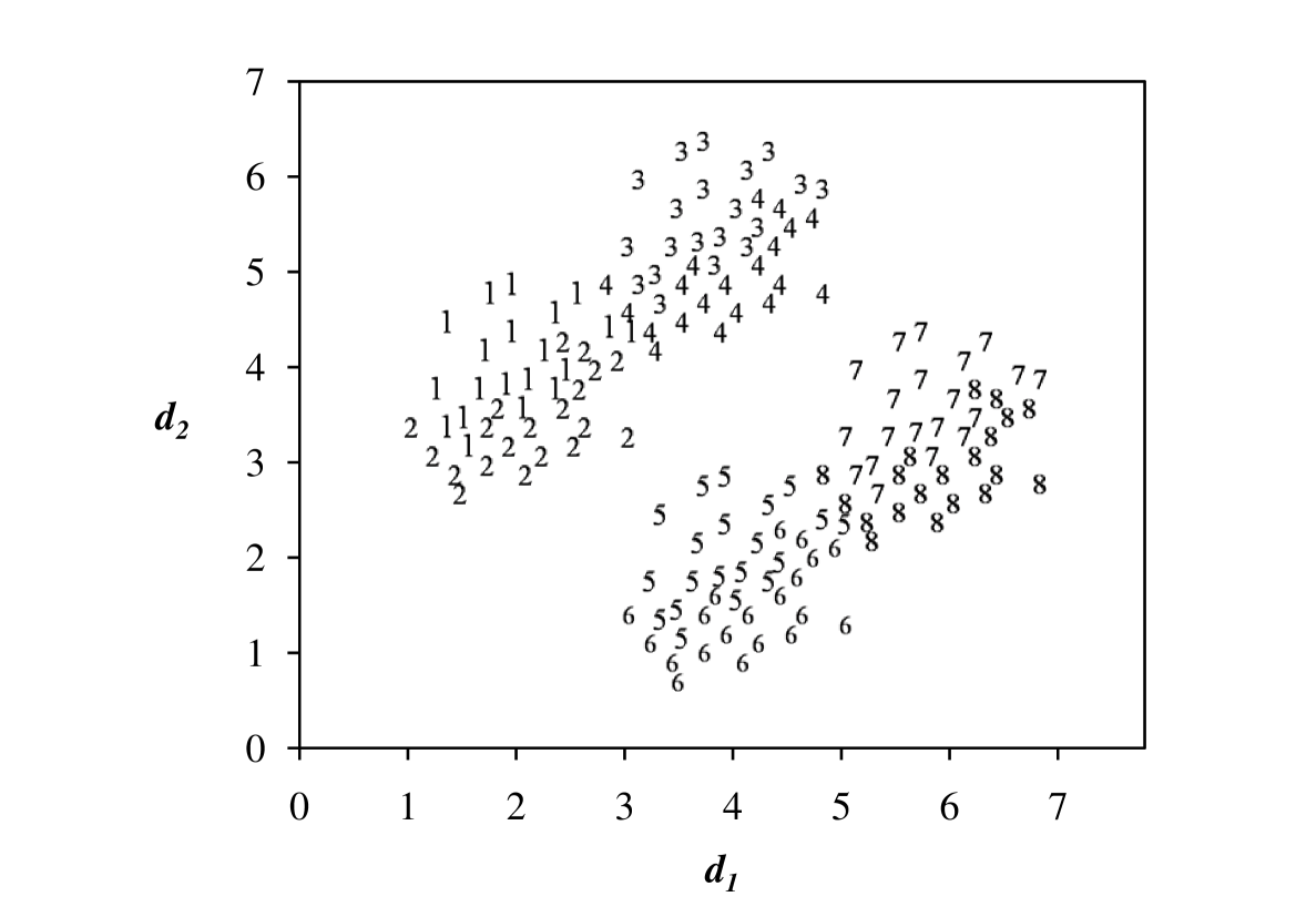
Figure 1: An example of two-dimensional artificial data including eight classes.

(a)

(b)

Figure 2: An example of the output of the minimum weight perfecting matching algorithm: (a) all possible matchings of eight subsets of classes and (b) an output of the matching algorithm.

Figure 3: An example of the code matrix constructed by the proposed method based on Linear Support Vector Machines with $C$ = 1 for the artificial data from Fig. 1 (The white region, the dark region, and the gray region represent $\textquoteleft$1’, $\textquoteleft$-1’, and $\textquoteleft$0’, respectively).

By the above reason, we carefully design the code matrix by considering the pairs of classes with hard separation as the first priority pairings and these pairings also indicate the high similarity between the classes. Intuitively, the pair of classes with difficult separation are allowed to combine with the low number of classes in order to avoid situation mentioned before, and we expect that the easier pairing can be combined with the large number of classes without affecting the classification ability much. Based on our idea, the classes with high similarity are grouped together as the same class label, and the classes with low similarity are separated. For example, consider two-dimensional artificial data shown in Fig. 1; classes 1,2,3,4 have high similarity and should be assigned with the same label (e.g. positive class), and classes 5,6,7,8 also have high similarity and should be assigned with the same label (e.g. negative class). Additionally, these two groups have low similarity by observation, and thus if we learn the binary model with a linear function, we will obtain absolutely separable hyperplane.

In order to obtain the code matrix satisfying the above requirements, we employ the minimum weight perfect matching algorithm [13] applied to find the optimal pairs of subset of classes by using the generalization performance [12] as a weighting criterion. Our method is called optimal matching of subset of classes algorithm described in Algorithm 1.

For solving the optimal matching problem, let $G=(V,E)$ be a graph with node set $V$ and edge set $E$. Each node in $G$ denotes one subset of classes and each edge indicates one binary classifier of which generalization performance is estimated from Algorithm 2 (see Fig. 2(a)). The output of the matching algorithm for graph $G$ is a subset of edges with the minimum sum of generalization performances of all edges and each node in $G$ is met by exactly one edge in the subset (see Fig. 2(b)).

Given a real weight $w_{e}$ being generalization performance for each edge $e$ of $G$, the problem of matching algorithm can be solved by the minimum weight perfect matching that finds a perfect matching $M$ of minimum weight $\sum(w_{e}:e\in M)$.

For $U\subseteq V$, let $E(U)=\{(i,j):(i,j)\in E,i\in U,j\in U\}$. $E(U)$ is the set of edges with both endpoints in $U$. The set of edges incident to node $i$ in the node-edge incidence matrix is denoted by $\delta(i)$. The convex hull of perfect matchings on a graph $G=(V,E)$ with $|V|$ even is given by
      a) $x\in\{0,1\}^{m}$
      b) $\sum_{e\in\delta(v)}x_{e}=1$ for $v\in V$
      c) $\sum_{e\in E(U)}x_{e}\leq\lfloor\frac{|U|}{2}\rfloor$ for all odd sets $U\subseteq V$ with $|U|\geq 3$
where $|E|=m$, and $x_{e}=1$ ($x_{e}=0$) means that $e$ is (is not) in the matching. Hence, the minimum weight of a perfect matching (mp) is at least as large as the following value.

$$mp=min\sum_{e\in E}w_{e}x_{e}$$ (1)

where $x$ satisfies (a), (b), and (c). Therefore, the matching problem can be solved by the integer program in Eq. (1).

On each round of Algorithm 1, we consider a sub-problem including $|S|$ subsets of classes, and calculate optimal pairs of subsets of classes by using the minimum weight perfect matching algorithm. The cost function employed in the minimum weight perfect matching algorithm is the sum of generalization performance calculated from Algorithm 2 [14]. The obtained subsets of classes are then used as a column of the code matrix. Consider data on Fig. 1 and the designed code matrix in Fig. 3, at the first round, each element of $S$ contains only set of one class, and the size of $S$ is 8. After applying the minimum weight perfect matching algorithm, we get four optimal pairings, i.e., classifier 1 vs 2, classifier 3 vs 4, classifier 5 vs 6, and classifier 7 vs 8. All of optimal four pairs as binary classifiers are added into the columns of the code matrix, i.e., classifiers $h_{1}$ to $h_{4}$ (see Fig. 3). The set $S$ is re-assigned by the empty set. The classes from each pairing are combined together into the same subset and then are added into $S$ as new members. Currently, the size of $S$ is 4, so we continue the next round. After applying the minimum weight perfect matching algorithm, we get two optimal pairings, i.e., classifier 1,2 vs 3,4, and classifier 5,6 vs 7,8. These two optimal pairs as binary classifiers are added into the columns of the code matrix, i.e., classifiers $h_{5}$ to $h_{6}$. The set $S$ is re-assigned by the empty set again, and then the classes from each pairing are combined together into the same subset and then are added into $S$ as new members. Now, the size of $S$ is 2, so we exit the loop. After that, the last remaining two subsets (the first subset including classes 1,2,3,4 and the second subset including classes 5,6,7,8) are added into the last column of the code matrix as binary classifier, i.e., classifier $h_{7}$.

In our methodology, a pair of classes that already are paired will not be considered again. In the later round, the number of the members in $S$ increases. For example at the last round, $S_{1}\leftarrow\{1,2,3,4\}$ and $S_{2}\leftarrow\{5,6,7,8\}$. It seems that this leads to complexity for calculating the hyperplane to separate between $S_{1}$ and $S_{2}$. However, the remaining classes that can be paired trend to allow easier separation due to the combination of classes in the same subset of classes having high similarity (in Fig. 1, classes 1,2,3,4 are very close, and classes 5,6,7,8 are also close), while the possible sixteen pairings including 1 vs 5, 1 vs 6, 1 vs 7, 1 vs 8, 2 vs 5, …, 4 vs 8 contain classes with high dissimilarity. It illustrates that these sixteen pairings are encoded in only one binary classifier as the One-Versus-One requires sixteen binary classifiers. This example also confirms that based on our technique although the number of classes for constructing a binary model increases, each subset of positive and negative classes is combined appropriately, and this leads to effective separation.

IV Experiments

In this section, we design the experiment to evaluate the performance of the proposed method. We compare our method with the classic codes, i.e., the dense random code, the sparse random code [1, 2], and the One-Versus-One [3]. This section is divided into two parts as experimental settings, and results & discussions.

IV-A Experimental Settings

We run experiments on ten datasets from the UCI Machine Learning Repository [10]. For the datasets containing both training data and test data, we added up both of them into one set, and used 5-fold cross validation for evaluating the classification accuracy.

TABLE I: Description of the datasets used in the experiments.

Datasets	#Classes	#Features	#Cases
Segment	7	18	2,310
Arrhyth	9	255	438
Mfeat-factor	10	216	2,000
Optdigit	10	62	5,620
Vowel	11	10	990
Primary Tumor	13	15	315
Libras Movement	15	90	360
Soybean	15	35	630
Abalone	16	8	4,098
Spectrometer	21	101	475

TABLE II: A comparison of the classification accuracies by using the dense random code and the proposed method.

Data sets	Dense random code		Proposed method
Segment	91.018$\pm$0.112		92.857$\pm$0.159*
Arrhyth	64.626$\pm$0.246*		60.731$\pm$0.298
Mfeat-factor	97.073$\pm$0.228		97.050$\pm$0.188
Optdigit	99.034$\pm$0.056		99.093$\pm$0.075
Vowel	59.632$\pm$0.980		80.808$\pm$0.479*
Primary Tumor	43.931$\pm$0.567		44.127$\pm$1.085
Libras Movement	82.507$\pm$0.372		84.722$\pm$0.621*
Soybean	93.273$\pm$0.418		93.651$\pm$0.251
Abalone	23.126$\pm$0.012		26.940$\pm$0.152*
Spectrometer	50.428$\pm$0.420		57.474$\pm$1.080*

TABLE III: A comparison of the classification accuracies by using the sparse random code and the proposed method.

Data sets	Sparse random code		Proposed method
Segment	91.937$\pm$0.105		92.857$\pm$0.159*
Arrhyth	62.112$\pm$0.225*		60.731$\pm$0.298
Mfeat-factor	97.048$\pm$0.212		97.050$\pm$0.188
Optdigit	99.072$\pm$0.059		99.093$\pm$0.075
Vowel	61.986$\pm$0.951		80.808$\pm$0.479*
Primary Tumor	44.770$\pm$0.864		44.127$\pm$1.085
Libras Movement	83.421$\pm$0.311		84.722$\pm$0.621
Soybean	93.115$\pm$0.421		93.651$\pm$0.251
Abalone	24.311$\pm$0.023		26.940$\pm$0.152*
Spectrometer	52.670$\pm$0.433		57.474$\pm$1.080*

TABLE IV: A comparison of the classification accuracies by using the One-Versus-One and the proposed method.

Data sets	One-Versus-One		Proposed method
Segment	92.741$\pm$0.174		92.857$\pm$0.159
Arrhyth	60.502$\pm$0.161		60.731$\pm$0.298
Mfeat-factor	97.183$\pm$0.189		97.050$\pm$0.188
Optdigit	99.170$\pm$0.062		99.093$\pm$0.075
Primary Tumor	44.550$\pm$0.831		44.127$\pm$1.085
Vowel	80.909$\pm$0.258		80.808$\pm$0.479
Libras Movement	84.352$\pm$0.317		84.722$\pm$0.621
Soybean	92.989$\pm$0.422		93.651$\pm$0.251
Abalone	26.326$\pm$0.063		26.940$\pm$0.152
Spectrometer	57.193$\pm$0.775		57.474$\pm$1.080

TABLE V: A comparison of the number of binary classifiers among the difference methods.

Data sets	#classes	Dense	Sparse	One-Versus-One	Proposed
		random code	random code		method
Segment	7	29	43	21	6
Arrhyth	9	32	48	36	8
Mfeat-factor	10	34	50	45	9
Optdigit	10	34	50	45	9
Vowel	11	35	52	55	10
Primary Tumor	13	38	56	78	12
Libras Movement	15	40	59	105	14
Soybean	15	40	59	105	14
Abalone	16	40	60	120	15
Spectrometer	21	44	66	210	20

In these experiments, we scaled data to be in [-1,1]. In the training phase, we used software package $SVM^{light}$ version 6.02 [15, 16] to create the binary classifiers. The regularization parameter $C$ of 1 was applied for model construction; this parameter is used to trade off between error of the SVM on training data and margin maximization. We employed the RBF kernel $K(x_{i},x_{j})\equiv e^{-\gamma||{\bf x_{i}}-{\bf x_{j}}||^{2}}$, and applied the degree $\gamma=0.1$ to all datasets. For the dense random code and the sparse random code, ten code matrices were randomly generated by using a pseudo-random tool [17]. In case of sparse random codes, the probability 1/2 and 1/4 were applied to generate the bit of $\textquoteleft$0’, and the other bits, i.e.. $\textquoteleft$1’ and $\textquoteleft$-1’, respectively. For decoding process, we employed the attenuated euclidean decoding [11] by using $AED(x,y_{i})=\sqrt{\sum_{j=1}^{L}|y_{i}^{j}||x^{j}|(x^{j}-y_{i}^{j})^{2}}$ where $x$ is binary output vector and $y_{i}$ is a code word belonging to class $i$.

IV-B Results & Discussions

We compared the proposed method with three traditional techniques, i.e., the dense random code, the sparse random code, and the One-Versus-One. The comparison results are shown in Table II to Table IV in which all of datasets are sorted in ascending order by their number of classes. For each dataset, the best accuracy among these algorithms is illustrated in bold-face and the symbol ‘*’ means that the method gives the higher accuracy at 95 % confidence interval with one-tailed paired t-test.

The experimental results in Table II shows that the proposed method yields highest accuracy in almost all datasets. The results also show that, at $95$% confidence interval, the proposed technique performs statistically better than the dense random code in five datasets and there is only one data set, i.e., the Arrhyth that the proposed method does not archive the better result. The experimental results in Table III illustrates that the proposed method gives higher accuracy compared to the sparse random code in almost all datasets. The results also show that, at $95$% confidence interval, the proposed technique performs statistically better than the sparse random code in four datasets and there is only one data set, i.e., the Arrhyth that the proposed method does not provide the higher accuracy. The combination method with a few binary classifiers may be weaker compared with one with the large number of binary classifier. Our proposed method is carefully designed to find the proper combination of classes, and to create the binary classifiers with high efficiency. However, as our method takes a few binary classifiers, it is possible that this situation may occur as found in case of the Arrhyth dataset. Moreover, the classification performance also relates to the structure of the code matrix. We consider the size of search space that is proportional to $\frac{3^{N}-2^{N+1}+1}{2}$ where $N$ is the number of classes. The dense random code and the sparse random code which is independent to the selection of a code matrix, while our method tries to find a specific structure of code matrix according to the relation of generalization performance of their classes. In case of the low number of $N$ with the small size of search space, the random techniques may obtain a good solution while in case of the higher number of $N$ with the bigger size of search space their probabilities to reach an expected solution decrease proportional to the growth of $N$. In this aspect, our method based on utilization of generalization performance as a guideline to find a solution is not affected. However, by the above reason in case of the small number of classes the code matrix generated by a random technique with the larger number of binary models may lead to the better classification performance as in the Arrhyth dataset mentioned before. Next, the last classification results in Table IV shows that the proposed method gives a little better results compared to the One-Versus-One in several datasets, and there is no significant difference between these two methods at $95$% confidence interval.

Consider the characteristic of the obtained binary models by using our technique. Some binary classifiers include the large number of classes that seem to be complex to construct binary models with high accuracy (as the first important issue). For example, in case of the Spectrometer dataset including 21 classes, twenty binary classifiers are obtained. The number of classes containing in the binary classifier is varied from 2 to 21 classes. For some hard-separation parings, our method allows the binary classifiers with the low number of classes to be combined to avoid the situation mentioned in Section III (as the second important issue). The effects of these two issues to the designed code matrix can be observed via the classification accuracies. Among all algorithms based on this dataset, our code matrix gives the higher classification accuracies compared to the dense random code and the sparse random code, while providing a little better results compared to the One-Versus-One. Moreover, the experimental results confirm that generally our algorithm provides the better code matrix that the proper subsets of classes are combined.

We also compare the classification time (the number of binary classifiers employed) of the proposed method to the traditional works as shown in Table V. The results illustrate that the proposed technique requires comparatively low running time in all datasets especially, when the number of classes is relatively large. Our technique reduces large number of classification times compared to all previous works; the dense random code, the sparse random code, and the One-Versus-One require $\lceil 10log_{2}N\rceil$, $\lceil 15log_{2}N\rceil$, and $N(N-1)/2$, respectively while our framework needs only $N-1$ for $N$-class problems. Our code matrix construction requires the calculation of class matching using the minimum weight perfect matching that the estimation of generalization performances are employed as a weighting criterion. Although this process needs additional computation to estimate the weight values using $k$-fold cross validation, the task is conducted in the training phase, and not affecting the performance in the classification phase.

V Conclusion

We propose an algorithm to find the suitable combination of classes for creating the binary models in the ECOC framework by using the generalization performance as a relation measure among subset of classes. This measure is applied to obtain the set of the closest pairs of subset of classes via the minimum weight perfect matching algorithm in order to generate the columns of the code matrix. The proposed method gives higher performance both in terms of accuracy and classification times compared to the traditional methods, i.e., the dense random code and the sparse random code. Moreover, our approach requires significantly smaller number of binary classifiers while maintaining accuracy compared to the One-versus-One. However, the expected matchings of subset of classes are not possibly available in some cases because relation of their subset of classes may force to combine inappropriate subset of classes and it may lead to misclassification. We will further analyze to address this situation in our future work.

VI Acknowledgment

This research is supported by the Thailand Research Fund, Thailand.

References

- [1] T.G.Dietterich, and G.Bakiri. “Solving multiclass learning problems via error-correcting output codes,”Journal of Artificial Intelligence Research, vol. 2, pp. 263-286, 1995.
- [2] E.L.Allwein, R.E.Schapire, and Y.Singer. “Reducing multiclass to binary: a unifying approach for margin classifiers,”Journal of Machine Learning Research, vol.1, pp. 113-141, 2000.
- [3] T.Hastie, and R.Tibshirani. “Classification by pairwise grouping,”Neural Information Processing Systems, vol.26, pp. 451-471,1998.
- [4] V.Vapnik. Statistical learning theory, New York, Wiley, 1998.
- [5] L.I.Kuncheva. “Using diversity measures for generating error-correcting output codes in classifier ensembles,”Pattern Recognition Letters, vol.26, pp. 83-90, 2005.
- [6] A.C.Lorena, and A.C.P.L.F.Carvalho. “Evaluation functions for the evolutionary design of multiclass support vector machines,”International Journal of Computational Intelligence and Applications, vol.8, pp.53-68, 2009.
- [7] M.A.Bagheri, G.Montazer, and E.Kabir. “A subspace approach to error correcting output codes,”Pattern Recognition Letters, vol.34, pp.176-184, 2013.
- [8] V.Vapnik. The nature of statistical learning theory, London, UK, Springer-Verlag, 1995.
- [9] V.Vapnik. “An overview of statistical learning theory,”IEEE Transactions on Neural Networks, vol.10, pp.988-999, 1999.
- [10] C.Blake, E.Keogh, and C.Merz. UCI repository of machine learning databases, Department of Information and Computer Science, University of California, Irvine, 1998.
- [11] S.Escalera, O.Pujol, P.Radeva. “On the decoding process in ternary error correcting output codes,”IEEE Transactions on Pattern Analysis and Machine Intelligence, vol.32, pp.120-134, 2010.
- [12] P.Bartlett, and J.Shawe-Taylor. “Generalization performance of support vector machines and other pattern classifiers,”Advances in Kernel Methods - Support Vector Learning, MIT Press, pp.43-54, 1998.
- [13] W.Cook, and A.Rohe. “Computing minimum-weight perfect matchings,”INFORMS Journal on Computing, vol.11, pp.138-148, 1999.
- [14] T.Mitchell. Machine Learning, McGraw Hill, 1997.
- [15] T.Joachims. “Making large-scale SVM learning practical,”Advances in Kernel Methods - Support Vector Learning, MIT Press, pp.169-184, 1998.
- [16] T.Joachims, SVMlight, http://ais.gmd.de/~thorsten/svm_light, 1999.
- [17] Bagheri, M. A., Gao, Q. and Escalera, S. “Efficient pairwise classification using Local Cross Off strategy,”Proceedings of the 25th Canadian Conference on Artificial Intelligence, pp.25-36, 2012.