Near-separable Non-negative Matrix Factorization with $\ell_{1}$- and Bregman Loss Functions

Abstract

Recently, a family of tractable NMF algorithms have been proposed under the assumption that the data matrix satisfies a separability condition Donoho & Stodden (2003); Arora et al. (2012). Geometrically, this condition reformulates the NMF problem as that of finding the extreme rays of the conical hull of a finite set of vectors. In this paper, we develop several extensions of the conical hull procedures of Kumar et al. (2013) for robust ($\ell_{1}$) approximations and Bregman divergences. Our methods inherit all the advantages of Kumar et al. (2013) including scalability and noise-tolerance. We show that on foreground-background separation problems in computer vision, robust near-separable NMFs match the performance of Robust PCA, considered state of the art on these problems, with an order of magnitude faster training time. We also demonstrate applications in exemplar selection settings.

1 Introduction

The problem of non-negative matrix factorization (NMF) is to express a non-negative matrix $\mathbf{X}$ of size $m\times n$, either exactly or approximately, as a product of two non-negative matrices, $\mathbf{W}$ of size $m\times r$ and $\mathbf{H}$ of size $r\times n$. Approximate NMF attempts to minimize a measure of divergence between the matrix $\mathbf{X}$ and the factorization $\mathbf{W}\mathbf{H}$. The inner-dimension of the factorization $r$ is usually taken to be much smaller than $m$ and $n$ to get interpretable part-based representation of data Lee & Seung (1999). NMF is used in a wide range of applications, e.g., topic modeling and text mining, hyper-spectral image analysis, audio source separation, and microarray data analysis Cichocki et al. (2009).

The exact and approximate NMF problem is NP-hard. Hence, traditionally, algorithmic work in NMF has focused on treating it as an instance of non-convex optimization Cichocki et al. (2009); Lee & Seung (1999); Lin (2007); Hsieh & Dhillon (2011) leading to algorithms lacking optimality guarantees beyond convergence to a stationary point. Promising alternative approaches have emerged recently based on a separability assumption on the data Arora et al. (2012); Bittorf et al. (2012); Gillis & Vavasis (2012); Kumar et al. (2013); Esser et al. (2012) which enables the NMF problem to be solved efficiently and exactly. Under this assumption, the data matrix $\mathbf{X}$ is said to be $r$-separable if all columns of $\mathbf{X}$ are contained in the conical hull generated by a subset of $r$ columns of $\mathbf{X}$. In other words, if $\mathbf{X}$ admits a factorization $\mathbf{W}\mathbf{H}$ then the separability assumption states that the columns of $\mathbf{W}$ are present in $\mathbf{X}$ at positions given by an unknown index set $A$ of size $r$. Equivalently, the corresponding columns of the right factor matrix $\mathbf{H}$ constitute the $r\times r$ identity matrix, i.e., $\mathbf{H}_{A}=\mathbf{I}$. We refer to these columns indexed by $A$ as anchor columns.

The separability assumption was first investigated by Donoho & Stodden (2003) in the context of deriving conditions for uniqueness of NMF. NMF under separability assumption has been studied for topic modeling in text  Kumar et al. (2013); Arora et al. (2013) and hyper-spectral imaging Gillis & Vavasis (2012); Esser et al. (2012), and separability has turned out to be a reasonable assumption in these two applications. In the context of topic modeling where $\mathbf{X}$ is a document-word matrix and $\mathbf{W}$, $\mathbf{H}$ are document-topic and topic-word associations respectively, it translates to assuming that there is at least one word in every topic that is unique to itself and is not present in other topics.

Our starting point in this paper is the family of conical hull finding procedures called Xray introduced in Kumar et al. (2013) for near-separable NMF problems with Frobenius norm loss. Xray finds anchor columns one after the other, incrementally expanding the cone and using exterior columns to locate the next anchor. Xray has several appealing features: (i) it requires no more than $r$ iterations each of which is parallelizable, (ii) it empirically demonstrates noise-tolerance, (iii) it admits efficient model selection, and (iv) it does not require normalizations or preprocessing needed in other methods. However, in the presence of outliers or different noise characteristics, the use of Frobenius norm approximations is not optimal.

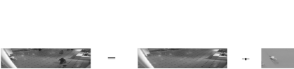
Figure 1: RobustXray applied to video background-foreground separation problem

In this paper, we extend Xray to provide robust factorizations with respect to $\ell_{1}$ loss, and approximations with respect to the family of Bregman divergences. Figure 1 shows a motivating application from computer vision. Given a sequence of video frames, the goal is to separate a near-stationary background from the foreground of moving objects that are relatively more dynamic across frames but span only a few pixels. In this setting, it is natural to seek a low-rank background matrix $\mathbf{B}$ that minimizes $\|\mathbf{X}-\mathbf{B}\|_{1}$ where $\mathbf{X}$ is the frame-by-pixel video matrix, and the $\ell_{1}$ loss imposes a sparsity prior on the residual foreground. Unlike the case of low-rank approximations in Frobenius or spectral norms, this problem does not admit an SVD-like tractable solution. The Robust Principal Component Analysis (RPCA), considered state of the art for this application, uses a nuclear-norm convex relaxation of the low-rank constraints. In this paper, we instead recover tractability by imposing the separable NMF assumption on the background matrix. This implies that the variability of pixels across the frames can be ”explained” in terms of observed variability in a small set of anchor pixels. Under a more restrictive setting, this can be shown to be equivalent to median filtering on the video frames, while a full near-separable NMF model imparts more degrees of freedom to model the background. We show that the proposed near-separable NMF algorithms with $\ell_{1}$ loss are competitive with RPCA in separating foreground from background while outperforming it in terms of computational efficiency.

Our algorithms are empirically shown to be robust to noise (deviations from the pure separability assumption). In addition to the background-foreground problem, we also demonstrate our algorithms on the exemplar selection problem. For identifying exemplars in a data set, the proposed algorithms are evaluated on text documents with classification accuracy as a performance metric and are shown to outperform the recently proposed method of Elhamifar et al. (2012).

Related Work: Existing separable NMF methods work either with only a limited number of loss functions on the factorization error such as Frobenius norm loss Kumar et al. (2013), $\ell_{1,\infty}$ norm loss Bittorf et al. (2012), or maximize proxy criteria such as volume of the convex polyhedron with anchor columns as vertices Gillis & Vavasis (2012) and distance between successive anchors Arora et al. (2013) to select the anchor columns. On the other hand, local search based NMF methods Cichocki et al. (2009) have been proposed for a wide variety of loss functions on the factorization error including $\ell_{1}$ norm loss Guan et al. (2012); Kim & Park (2007) and instances of Bregman divergence Li et al. (2012); Sra & Dhillon (2005). In this paper, we close this gap and propose algorithms for near-separable NMF that minimize $\ell_{1}$ loss and Bregman divergence for the factorization.

2 Geometric Intuition

The goal in exact NMF is to find a matrix $\mathbf{W}$ such that the cone generated by its columns (i.e., their non-negative linear combinations) contains all columns of $\mathbf{X}$. Under separability assumption, the columns of matrix $\mathbf{W}$ are to be picked directly from $\mathbf{X}$, also known as anchor columns. The algorithms in this paper build the cone incrementally by picking a column from $\mathbf{X}$ in every iteration. The algorithms execute $r$ such iterations for constructing a factorization of inner-dimension $r$. Figure 2 shows the cone after three iterations of the algorithm when three anchor columns have been identified. An extreme ray $\{t\mathbf{x}:t>0\}$ is associated with every anchor point $\mathbf{x}$. The points on an extreme ray cannot be expressed as conic combinations of other points in the cone that do not themselves lie on that extreme ray. To identify the next anchor column, the algorithm picks a point outside the current cone (a green point) and projects it to the current cone so that the distance between the point and the projection is minimized in terms of the desired measure of distance. This projection is then used to setup a specific simple criteria which when maximized over the data points, identifies a new anchor. This new anchor is then added to the current set of anchors and the cone is expanded iteratively until all anchors have been picked.

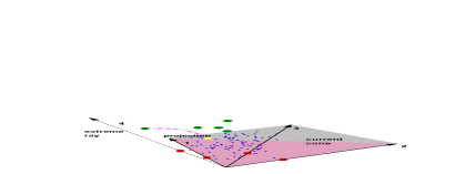
Figure 2: Geometrical illustration of the algorithm

These geometric intuitions are inspired by Clarkson (1994); Dula et al. (1998) who present linear programming (LP) based algorithms for general convex and conical hull problems. Their algorithms use $\ell_{2}$ projections of exterior points to the current cone and are also applicable in our NMF setting if the data matrix $\mathbf{X}$ satisfies $r$-separability exactly. In this case, the $\ell_{2}$ projection and corresponding residual vector of any single exterior point can be used to expand the cone and all $r$ anchors will be recovered correctly at the end of the algorithm. When $\mathbf{X}$ does not satisfy $r$-separability exactly, anchor selection criteria derived from multiple residuals demonstrate superior noise robustness as empirically shown by Kumar et al. (2013) who consider the case of Gaussian i.i.d. noise. However, the algorithms of Kumar et al. (2013) are not suitable for noise distributions other than Gaussian (e.g., other members of the exponential family, sparse noise) as they minimize $\lVert\mathbf{X}-\mathbf{X}_{A}\mathbf{H}\rVert_{\mathrm{F}}^{2}$. In the following sections, we present algorithms for near-separable NMF that are targeted precisely towards this goal and empirically demonstrate their superiority over existing algorithms under different noise distributions.

3 Near-separable NMF with $\ell_{1}$ loss

This section considers the case when the pure separable structure is perturbed by sparse noise. Hence our aim is to minimize $\lVert\mathbf{X}-\mathbf{X}_{A}\mathbf{H}\rVert_{1}$ for $\mathbf{H}\geq 0$ where $\lVert\cdot\rVert_{1}$ denotes element-wise $\ell_{1}$ norm of the matrix and $\mathbf{X}_{A}$ are the columns of $\mathbf{X}$ indexed by set $A\subset\{1,2,\ldots,n\}$. We denote $i$th column of $\mathbf{X}$ by $\mathbf{X}_{i}$. The proposed algorithm proceeds by identifying one anchor column in each iteration and adding it to the current set of anchors, thus expanding the cone generated by anchors. Each iteration consists of two steps: (i) anchor selection step that finds the column of $\mathbf{X}$ to be added as an anchor, and (ii) a projection step where all data points (columns of $\mathbf{X}$) are projected to the current cone in terms of minimizing the $\ell_{1}$ norm. Algorithm 1 outlines the steps of the proposed algorithm.

Selection Step: In the selection step, we normalize all the points to lie on the hyperplane $\mathbf{p}^{T}\mathbf{x}=1$ ($\mathbf{Y}_{j}=\frac{\mathbf{X}_{j}}{\mathbf{p}^{T}\mathbf{X}_{j}}$) for a strictly positive vector $\mathbf{p}$ and evaluate the selection criterion of Eq. 3 to select the next anchor column. Note that any exterior point ($i:\|\mathbf{R}_{i}\|_{1}\geq 0$) can be used in the selection criterion – Algorithm 1 shows two possibilities for choosing the exterior point. Taking the point with maximum residual $\ell_{1}$ norm to be the exterior point turns out to be far more robust to noise than randomly choosing the exterior point, as observed in our numerical simulations.

Projection Step: The projection step, Eq. 4, involves solving a multivariate least absolute devitations problems with non-negativity constraints. We we use alternating direction method of multipliers (ADMM) Boyd et al. (2011) and reformulate the problem as

$$\min_{B\geq 0,\mathbf{Z}}\|\mathbf{Z}\|_{1},\text{ such that}~{}\mathbf{X}_{A}\mathbf{B}+\mathbf{Z}=\mathbf{X}.$$

Thus the non-negativity constraints are decoupled from the $\ell_{1}$ objective and the ADMM optimization proceeds by alternating between two sub-problems – a standard $\ell_{1}$ penalized $\ell_{2}$ proximity problem in variable $\mathbf{Z}$ which has a closed form solution using the soft-thresholding operator, and a non-negative least squares problem in variable $\mathbf{B}$ that is solved using a cyclic coordinate descent approach (cf. Algorithm 2 in Kumar et al. (2013)). The standard primal and dual residuals based criteria is used to declare convergence Boyd et al. (2011). The ADMM procedure converges to the global optimum since the problem is convex.

Algorithm 1 RobustXray: Near-separable NMF with $\ell_{1}$ loss

  Input: $\mathbf{X}\in\mathbb{R}_{+}^{m\times n}$, inner dimension $r$

  Output: $\mathbf{W}\in\mathbb{R}_{m\times r},\mathbf{H}\in\mathbb{R}_{r\times n}$, $r$ indices in $A$             such that: $\mathbf{X}=\mathbf{W}\mathbf{H}$, $\mathbf{W}=\mathbf{X}_{A}$

  Initialize: $\mathbf{R}\leftarrow\mathbf{X}$, $\mathbf{D}^{\star}\leftarrow\mathbf{X}$, $A\leftarrow\{\}$

  while $|A|<r$ do

     1. Anchor Selection step:

     First, pick any point exterior to the current cone. Two possible criteria are

$$\textrm{{rand}}: ~{}~{}\textrm{any random}~{}~{}i:\|\mathbf{R}_{i}\|_{1}>0$$ (1)

$$\textrm{{max}}: i=\mathop{\rm arg\,max}_{k}\|\mathbf{R}_{k}\|_{1}$$ (2)

     Choose a suitable $\mathbf{D}_{i}^{\star}\in\mathbf{D}_{i}$ where $\mathbf{D}_{ji}=sign(\mathbf{R}_{ji})$ if $\mathbf{R}_{ji}\neq 0$, else $\mathbf{D}_{ji}\in[-1,1]$ (see Remark (1)).

     Select an anchor as follows ($\mathbf{p}$ is a strictly positive vector, not collinear with $\mathbf{D}_{i}^{\star}$ (see Remark (3))):

$$j^{\star}=\mathop{\rm arg\,max}_{j}\frac{\mathbf{D}_{i}^{\star^{T}}\mathbf{X}_{j}}{\mathbf{p}^{T}\mathbf{X}_{j}}$$ (3)

     2. Update: $A\leftarrow A\cup\{j^{\star}\}$ (see Remark (2))

     3. Projection step: Project onto current cone.

$$\mathbf{H}=\mathop{\rm arg\,min}_{\mathbf{B}\geq 0}\|\mathbf{X}-\mathbf{X}_{A}\mathbf{B}\|_{1}~{}~{}~{}~{}\text{(ADMM)}$$ (4)

     4. Update Residuals:    $\mathbf{R}=\mathbf{X}-\mathbf{X}_{A}\mathbf{H}$

  end while

We now show that Algorithm 1 correctly identifies all the anchors in pure separble case.

Lemma 3.1.

Let $\mathbf{R}$ be the residual matrix obtained after $\ell_{1}$ projection of columns of $\mathbf{X}$ onto the current cone and $\mathbf{D}$ be the set of matrices such $\mathbf{D}_{ij}=sign(\mathbf{R}_{ij})$ if $\mathbf{R}_{ij}\neq 0$ else $\mathbf{D}_{ij}\in[-1,1]$. Then, there exists at least one $\mathbf{D}^{\star}\in\mathbf{D}$ such that $\mathbf{D}^{\star^{T}}\mathbf{X}_{A}\leq 0$, where $\mathbf{X}_{A}$ are anchor columns selected so far by Algorithm 1.

Proof.

Residuals are given by $\mathbf{R}=\mathbf{X}-\mathbf{X}_{A}\mathbf{H}$, where $\mathbf{H}=\mathop{\rm arg\,min}_{\mathbf{B}\geq 0}\lVert\mathbf{X}-\mathbf{X}_{A}\mathbf{B}\rVert_{1}$.
Forming the Lagrangian for Eq. 4, we get $\mathcal{L}(\mathbf{B},\bm{\Lambda})=\lVert\mathbf{X}-\mathbf{X}_{A}\mathbf{B}\rVert_{1}-tr(\bm{\Lambda}^{T}\mathbf{B})$, where the matrix $\bm{\Lambda}$ contains the non-negative Lagrange multipliers. The Lagrangian is not smooth everywhere and its sub-differential is given by $\partial\mathcal{L}=-\mathbf{X}_{A}^{T}\mathbf{D}-\bm{\Lambda}$ where $\mathbf{D}$ is as defined in the lemma. At the optimum $\mathbf{B}=\mathbf{H}$, we have $0\in\partial\mathcal{L}$ $\Rightarrow-\bm{\Lambda}\in\mathbf{X}_{A}^{T}\mathbf{D}$. Since $\bm{\Lambda}\geq 0$, this means that there exists at least one $\mathbf{D}^{\star}\in\mathbf{D}$ for which $\mathbf{D}^{\star^{T}}\mathbf{X}_{A}\leq 0$. ∎

Lemma 3.2.

For any point $\mathbf{X}_{i}$ exterior to the current cone, there exists at least one $\mathbf{D}^{\star}\in\mathbf{D}$ such that it satisfies the previous lemma and $\mathbf{D}_{i}^{\star^{T}}\mathbf{X}_{i}>0$.

Proof.

Let $\mathbf{R}=\mathbf{X}-\mathbf{X}_{A}\mathbf{H}$, where $\mathbf{H}=\mathop{\rm arg\,min}_{\mathbf{B}\geq 0}\lVert\mathbf{X}-\mathbf{X}_{A}\mathbf{B}\rVert_{1}$ and $\mathbf{X}_{A}$ are the current set of anchors. From the proof of previous lemma, $-\bm{\Lambda}^{T}\in\mathbf{D}^{T}\mathbf{X}_{A}$. Hence, $-\bm{\Lambda}_{i}^{T}\in\mathbf{D}_{i}^{T}\mathbf{X}_{A}$ ($i$th row of both left and right side matrices). From the complementary slackness condition, we have $\bm{\Lambda}_{ji}\mathbf{H}_{ji}=0\,\,\forall\,j,i$. Hence, $-\bm{\Lambda}_{i}^{T}\mathbf{H}_{i}=0\in\mathbf{D}_{i}^{T}\mathbf{X}_{A}\mathbf{H}_{i}$.
Since all KKT conditions are met at the optimum, there is at least one $\mathbf{D}^{\star}\in\mathbf{D}$ that satisfies previous lemma and for which $\mathbf{D}_{i}^{\star^{T}}\mathbf{X}_{A}\mathbf{H}_{i}=0$. For this $\mathbf{D}^{\star}$, we have $\mathbf{D}_{i}^{\star^{T}}\mathbf{X}_{i}=\mathbf{D}_{i}^{\star^{T}}(\mathbf{R}_{i}+\mathbf{X}_{A}\mathbf{H}_{i})=\mathbf{D}_{i}^{\star^{T}}\mathbf{R}_{i}=\lVert\mathbf{R}_{i}\rVert_{1}>0$ since $\mathbf{R}_{i}\neq 0$ for an exterior point. ∎

Using the above two lemmas, we prove the following theorem regarding the correctness of Algorithm 1 in pure separable case.

Theorem 3.1.

If the maximizer in Eq. 3 is unique, the data point $\mathbf{X}_{j^{\star}}$ added at each iteration in the Selection step of Algorithm 1, is an anchor that has not been selected in one of the previous iterations.

Proof.

Let the index set $A$ denote all the anchor columns of $\mathbf{X}$. Under the separability assumption, we have $\mathbf{X}=\mathbf{X}_{A}\mathbf{H}$. Let the index set $A^{t}$ identify the current set of anchors.

Let $\mathbf{Y}_{j}=\frac{\mathbf{X}_{j}}{\mathbf{p}^{T}\mathbf{X}_{j}}$ and $\mathbf{Y}_{A}=\mathbf{X}_{A}[diag(\mathbf{p}^{T}\mathbf{X}_{A})]^{-1}$ (since $\mathbf{p}$ is strictly positive, the inverse exists). Hence $\mathbf{Y}_{j}=$ $\mathbf{Y}_{A}\frac{[diag(\mathbf{p}^{T}\mathbf{X}_{A})]\mathbf{H}_{j}}{\mathbf{p}^{T}\mathbf{X}_{j}}$. Let $\mathbf{C}_{j}=\frac{[diag(\mathbf{p}^{T}\mathbf{X}_{A})]\mathbf{H}_{j}}{\mathbf{p}^{T}\mathbf{X}_{j}}$. We also have $\mathbf{p}^{T}\mathbf{Y}_{j}=1$ and $\mathbf{p}^{T}\mathbf{Y}_{A}=\mathbf{1}^{T}$. Hence, we have $1=\mathbf{p}^{T}\mathbf{Y}_{j}=\mathbf{p}^{T}\mathbf{Y}_{A}\mathbf{C}_{j}=\mathbf{1}^{T}\mathbf{C}_{j}$.

Using Lemma 3.1, Lemma 3.2 and the fact that $\mathbf{p}$ is strictly positive, we have $\max_{1\leq j\leq n}\mathbf{D}_{i}^{\star^{T}}\mathbf{Y}_{j}=\max_{j\notin A^{t}}\mathbf{D}_{i}^{\star^{T}}\mathbf{Y}_{j}$. Indeed, for all $j\in A^{t}$ we have $\mathbf{D}_{i}^{\star^{T}}\mathbf{Y}_{j}\leq 0$ using Lemma 3.1 and there is at least one $j=i\notin A^{t}$ for which $\mathbf{D}_{i}^{\star^{T}}\mathbf{Y}_{j}>0$ using Lemma 3.2. Hence the maximum lies in the set $\{j:j\notin A^{t}\}$.

Further, we have $\max_{j\notin A^{t}}\mathbf{D}_{i}^{\star^{T}}\mathbf{Y}_{j}=\max_{j\notin A^{t}}\mathbf{D}_{i}^{\star^{T}}\mathbf{Y}_{A}\mathbf{C}_{j}\leq\max_{j\in(A\setminus A^{t})}\mathbf{D}_{i}^{\star^{T}}\mathbf{Y}_{j}$. The second inequality is the result of the fact that $\lVert\mathbf{C}_{j}\rVert_{1}=1$ and $\mathbf{C}_{j}\geq 0$. This implies that if there is a unique maximum at a $j^{*}=\mathop{\rm arg\,max}_{j\notin A^{t}}\mathbf{D}_{i}^{\star^{T}}\mathbf{Y}_{j}$, then $\mathbf{X}_{j^{*}}$ is an anchor that has not been selected so far. ∎

Remarks:

(1) For the correctness of Algorithm 1, the anchor selection step requires choosing a $\mathbf{D}_{i}^{\star}\in\mathbf{D}_{i}$ for which Lemma 3.1 and Lemma 3.2 hold true. Here we give a method to find one such $\mathbf{D}_{i}^{\star}$ using linear programming. Using KKT conditions, the $\mathbf{D}_{i}^{\star}$ satisfying $-\mathbf{X}_{A}^{T}\mathbf{D}_{i}^{\star}=\bm{\Lambda}_{i}\in\mathbb{R}_{+}^{|A|}$ is a candidate. We know $\bm{\Lambda}_{ji}=0$ if $\mathbf{H}_{ji}>0$ and $\bm{\Lambda}_{ji}>0$ if $\mathbf{H}_{ji}=0$ (complementary slackness). Let $Z=\{j:\mathbf{H}_{ji}>0\}$ and $\widetilde{Z}=\{j:\mathbf{H}_{ji}=0\}$. Let $I=\{j:\mathbf{R}_{ji}=0\}$. Let $\mathbf{u}$ represent the elements of $\mathbf{D}_{i}^{\star}$ that we need to find, i.e., $\mathbf{u}=\{\mathbf{D}_{ji}^{\star}:j\in I\}$. Finding $\mathbf{u}$ is a feasibility problem that can be solved using an LP. Since there can be multiple feasible points, we can choose a dummy cost function $\sum_{k}\mathbf{u}_{k}$ (or any other random linear function of $\mathbf{u}$) for the LP. More formally, the LP takes the form:

$$~{}~{}~{}~{}~{}~{}~{}~{}~{}~{}\min_{-1\leq\mathbf{u}\leq 1}\mathbf{1}^{T}\mathbf{u},~{}~{}~{}\text{such that}$$

$$-\mathbf{X}_{A}^{T}\mathbf{D}_{i}^{\star}=\bm{\Lambda}_{i},\bm{\Lambda}_{ji}=0~{}\forall~{}j\in Z,\bm{\Lambda}_{ji}>0~{}\forall~{}j\in\widetilde{Z}\vspace{-3mm}$$

In principle, the number of variables in this LP is the number of zero entries in residual vector $\mathbf{R}_{i}$ which can be as large as $m-1$. In practice, we always have the number of zeros in $\mathbf{R}_{i}$ much less than $m$ since we always pick the exterior point with maximum $\ell_{1}$ norm in the Anchor Selection step of Algorithm 1. The number of constraints in the LP is also very small ($=|A|<r)$. In our implementation, we simply set $\mathbf{u}=-1$ which, in practice, almost always satisfies Lemma 3.1 and Lemma 3.2. The LP is called whenever Lemma 3.2 is violated which happens rarely (note that Lemma 3.1 will never violate with this setting of $\mathbf{u}$).

(2) If the maximum of Eq. 3 occurs at two points $j_{1}^{*}$ and $j_{2}^{*}$, both these points $\mathbf{X}_{j_{1}^{*}}$ and $\mathbf{X}_{j_{2}^{*}}$ generate the extreme rays of the data cone. Hence both are added to anchor set $A$. If the maximum occurs at more than two points, some of these are the anchors and others are conic combinations of these anchors. We can identify the anchors of this subset of points by calling Algorithm 1 recursively.

(3) In Algorithm 1, the vector $\mathbf{p}$ needs to satisfy $\mathbf{p}^{T}\mathbf{x}_{i}>0,i=1\ldots n$. In our implementation, we simply used $\mathbf{p}=\mathbf{1}+\bm{\delta}\in\mathbb{R}^{m}$ where $\bm{\delta}$ is small perturbation vector with entries i.i.d. according to a uniform distribution $\mathcal{U}(0,10^{-5})$. This is done to avoid the possibility of $\mathbf{p}$ being collinear with $\mathbf{D}_{i}^{\star}$.

4 Near-separable NMF with Bregman divergence

Let $\phi:\mathcal{S}\mapsto\mathbb{R}$ be a strictly convex function on domain $\mathcal{S}\subseteq\mathbb{R}$ which is differentiable on its non-empty relative interior $ri(\mathcal{S})$. Bregman divergence is then defined as $D_{\phi}(x,y)=\phi(x)-\phi(y)-\phi^{\prime}(y)(x-y)$ where $\phi^{\prime}(y)$ is the continuous first derivative of $\phi(\cdot)$ at $y$. Here we will also assume $\phi^{\prime}(\cdot)$ to be smooth which is true for most Bregman divergences of interest. A Bregman divergence is always convex in the first argument. Some instances of Bregman divergence are also convex in the second argument (e.g., KL divergence). For two matrices $\mathbf{X}$ and $\mathbf{Y}$, we work with divergence of the form $D_{\phi}(\mathbf{X},\mathbf{Y}):=\sum_{ij}D_{\phi}(\mathbf{X}_{ij},\mathbf{Y}_{ij})$.

Here we consider the case when the entries of data matrix $\mathbf{X}$ are generated from an exponential family distribution with parameters satisfying the separability assumption, i.e., $\mathbf{X}_{ij}\sim\mathcal{P}_{\phi}(\mathbf{W}^{i}\mathbf{H}_{j}),~{}\mathbf{W}\in\mathbb{R}_{+}^{m\times r},\mathbf{H}=[\mathbf{I}\,\,\mathbf{H}^{\prime}]\in\mathbb{R}_{+}^{r\times n}$ ($\mathbf{W}^{i}$ and $\mathbf{H}_{j}$ denote the $i$th row of $\mathbf{W}$ and the $j$th column of $\mathbf{H}$, respectively). Every member distribution $\mathcal{P}_{\phi}$ of the exponential family has a unique Bregman divergence $D_{\phi}(\cdot,\cdot)$ associated with it Banerjee et al. (2005), and solving $\min_{\mathbf{Y}}D_{\phi}(\mathbf{X},\mathbf{Y})$ is equivalent to maximum likelihood estimation for parameters $\mathbf{Y}_{ij}$ of the distribution $\mathcal{P}_{\phi}(\mathbf{Y}_{ij})$. Hence, the projection step in Algorithm 1 is changed to $\mathbf{H}=\mathop{\rm arg\,min}_{\mathbf{B}\geq 0}D_{\phi}(\mathbf{X},\mathbf{X}_{A}\mathbf{B})$. We use the coordinate descent based method of Li et al. (2012) to solve the projection step. To select the anchor columns with Bregman projections $\mathbf{X}_{A}\mathbf{H}$, we modify the selection criteria as

$$j^{\star}=\mathop{\rm arg\,max}_{j}\frac{(\phi^{\prime\prime}(\mathbf{X}_{A}\mathbf{H}_{i})\odot\mathbf{R}_{i})^{T}\mathbf{X}_{j}}{\mathbf{p}^{T}\mathbf{X}_{j}}$$ (5)

for any $i:\|\mathbf{R}_{i}\|>0$, where $\mathbf{R}=\mathbf{X}-\mathbf{X}_{A}\mathbf{H}$ and $\phi^{\prime\prime}(\mathbf{x})$ is the vector of second derivatives of $\phi(\cdot)$ evaluated at individual elements of the vector $\mathbf{x}$ (i.e., $[\phi^{\prime\prime}(\mathbf{x})]_{j}=\phi^{\prime\prime}(\mathbf{x}_{j})$), and $\odot$ denotes element-wise product of vectors. We can show the following result regarding the anchor selection property of this criteria. Recall that an anchor is a column that can not be expressed as conic combination of other columns in $\mathbf{X}$.

Theorem 4.1.

If the maximizer of Eq. 5 is unique, the data point $\mathbf{X}_{j^{\star}}$ added at each iteration in the Selection step, is an anchor that has not been selected in one of the previous iterations.

The proof is provided in the Appendix. Again, any exterior point $i$ can be chosen to select the next anchor but our simulations show that taking exterior point to be $i=\mathop{\rm arg\,max}_{k}D_{\phi}(\mathbf{X}_{k},\mathbf{X}_{A}\mathbf{H}_{k})$ gives much better performance under noise than randomly choosing the exterior point. Note that for the Bregman divergence induced by function $\phi(x)=x^{2}$, the selection criteria of Eq. 5 reduces to the selection criteria of Xray  proposed in Kumar et al. (2013).

Since Bregman divergence is not generally symmetric, it is also possible to have the projection step as $\mathbf{H}=\mathop{\rm arg\,min}_{\mathbf{B}\geq 0}D_{\phi}(\mathbf{X}_{A}\mathbf{B},\mathbf{X})$. In this case, the selection criteria will change to $j^{\star}=\mathop{\rm arg\,max}_{j}\frac{(\phi^{\prime}(\mathbf{X}_{i})-\phi^{\prime}(\mathbf{X}_{A}\mathbf{H}_{i}))^{T}\mathbf{X}_{j}}{\mathbf{p}^{T}\mathbf{X}_{j}}$ for any point $i$ exterior to the current cone, where $\phi^{\prime}(\mathbf{x})$ operates element-wise on vector $\mathbf{x}$. However this variant does not have as meaningful a probabilistic interpretation as the one discussed earlier.

5 Empirical Observations

In this section, we present experiments on synthetic and real datasets to demonstrate the effectiveness of the proposed algorithms under noisy conditions. In addition to comparing our algorithms with existing separable NMF methods Bittorf et al. (2012); Gillis & Vavasis (2012); Kumar et al. (2013), we also benchmark them against Robust PCA and local-search based low-rank factorization methods, wherever applicable, for the sake of providing a more complete picture.

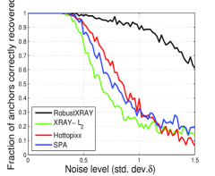
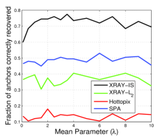
Figure 3: Left: Anchor recovery rate versus noise level for sparse noise case, Right: Anchor recovery rate versus mean parameter for data matrix generated from exponential distribution (best viewed in color)

5.1 Anchor recovery under noise

Here we test the proposed algorithms for recovery of anchors when the separable structure is perturbed by noise. We compare with methods proposed in Gillis & Vavasis (2012) (abbrv. as SPA for Successive Projection Approximation), Bittorf et al. (2012) (abbrv. as Hottopixx ) and Kumar et al. (2013) (abbrv. as Xray-$\ell_{2}$ ).

First, we consider the case when the separable structure is perturbed by addition of a sparse noise matrix, i.e., $\mathbf{X}=\mathbf{W}\mathbf{H}+\mathbf{N},~{}\mathbf{H}=[\mathbf{I}\,\,\mathbf{H}^{\prime}]$. Each entry of matrix $\mathbf{W}\in\mathbb{R}_{+}^{200\times 20}$ is generated i.i.d. from a uniform distribution between $0$ and $1$. The matrix $\mathbf{H}\in\mathbb{R}^{20\times 210}$ is taken to be $[\mathbf{I}_{20\times 20}\,\,\mathbf{H}^{\prime}_{20\times 190}]$ where each column of $\mathbf{H}^{\prime}$ is sampled i.i.d. from a Dirichlet distribution whose parameters are generated i.i.d. from a uniform distribution between $0$ and $1$. It is clear from the structure of matrix $\mathbf{H}$ that first twenty columns are the anchors. The data matrix $\mathbf{X}$ is generated as $\mathbf{W}\mathbf{H}+\mathbf{N}$ with $\mathbf{N}=\max(\mathbf{N}_{1},0)\in\mathbb{R}_{+}^{200\times 210}$, where each entry of $\mathbf{N}_{1}$ is generated i.i.d. from a Laplace distribution having zero mean and $\delta$ standard deviation. Since Laplace distribution is symmetric around mean, almost half of the entries in matrix $\mathbf{N}$ are $0$ due to the $\max$ operation. The std. dev. $\delta$ is varied from $0$ to $1.5$ with a step size of $0.02$. Fig. 3 plots the fraction of correctly recovered anchors averaged over $10$ runs for each value of $\delta$. The proposed RobustXray  (Algorithm 1) outperforms all other methods including Xray-$\ell_{2}$ by a huge margin as the noise level increases. This highlights the importance of using the right loss function in the projection step that is suitable for the noise model (in this case $\ell_{1}$ loss of Eq. 4).

Next, we consider the case where the non-negative data matrix is generated from an exponential family distribution other than the Gaussian, i.e., $\mathbf{X}_{ij}\sim\mathcal{P}_{\phi}(\mathbf{W}^{i}\mathbf{H}_{j}),~{}\mathbf{W}\in\mathbb{R}_{+}^{m\times r},\mathbf{H}=[\mathbf{I}\,\,\mathbf{H}^{\prime}]\in\mathbb{R}_{+}^{r\times n}$ ($\mathbf{W}^{i}$ and $\mathbf{H}_{j}$ denote the $i$th row of $\mathbf{W}$ and the $j$th column of $\mathbf{H}$, respectively). As mentioned earlier, every member distribution $\mathcal{P}_{\phi}$ of the exponential family has a unique Bregman divergence $D_{\phi}$ associated with it. Hence we minimize the corresponding Bregman divergence in the projection step of the algorithm as discussed in Section 4, to recover the anchor columns. Two most commonly used Bregman divergences are generalized KL-divergence and Itakura-Saito (IS) divergence Sra & Dhillon (2005); Banerjee et al. (2005); Févotte et al. (2009) that correspond to Poisson and Exponential distributions, respectively. We do not report results with generalized KL-divergence here since they were not very informative in highlighting the differences among various algorithms that are considered. The reason is that Poisson distribution with parameter $\lambda$ has a mean of $\lambda$ and std. dev. of $\sqrt{\lambda}$, and increasing the noise (std. dev.) actually increases the signal to noise ratio. Hence anchor recovery gets better with increasing $\lambda$ (perfect recovery after certain value) and almost all algorithms perform as well as Xray-KL for the full $\lambda$ range. The anchor recovery results with IS-divergence are shown in Fig. 3. The entries of data matrix $\mathbf{X}$ are generated as $\mathbf{X}_{ij}\sim\exp(\lambda\mathbf{W}^{i}\mathbf{H}_{j})~{}\mathbf{W}\in\mathbb{R}_{+}^{200\times 20},\mathbf{H}=[\mathbf{I}_{20\times 20}\,\,\mathbf{H}^{\prime}]\in\mathbb{R}_{+}^{20\times 210}$. The matrices $\mathbf{W}$ and $\mathbf{H}$ are generated as described in the previous paragraph. The parameter $\lambda$ is varied from $0$ to $10$ in the steps of $0.5$ and we report the average over $10$ runs for each value of $\lambda$. The Xray-IS algorithm significantly outperforms other methods including Xray-$\ell_{2}$  Kumar et al. (2013) in correctly recovering the anchor column indices. The recovery rate does not change much with increasing $\lambda$ since exponential distribution with mean parameter $\lambda$ has a std. dev. of $\lambda$ and the signal-to-noise ratio practically stays almost same with varying $\lambda$.

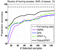
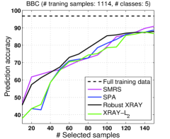
Figure 4: Accuracy of SVM trained with selected exemplars on Reuters data (left) and BBC data (right) (best viewed in color)

5.2 Exemplar Selection

The problem of exemplar selection is concerned with finding a few representatives from a dataset that can summarize the dataset well. Exemplar selection can be used in many applications including summarizing a video sequence, selecting representative images or text documents (e.g., tweets) from a collection, etc. If $\mathbf{X}$ denotes the data matrix where each column is a data point, the exemplar selection problem translates to selecting a few columns from $\mathbf{X}$ that can act as representatives for all the columns. The separable NMF algorithms can be used for this task, working under the assumption that all data points (columns of $\mathbf{X}$) can be expressed as non-negative linear combinations of the exemplars (the anchor columns). To be able to compare the quality of the selected exemplars by different algorithms in an objective manner, we test them on a classification task (assuming that every data point has an associated label). We randomly partition the data in training and test sets, and use only training set in selecting the exemplars. We train a multiclass SVM classifier Fan et al. (2008) with the selected exemplars and look at its accuracy on the held-out test set. The accuracy of the classifier trained with the full training set is taken as a benchmark and is also reported. We also compare with Elhamifar et al. (2012) who recently proposed a method for exemplar selection, named as Sparse Modeling Representative Selection (SMRS). They assume that the data points can be expressed as a convex linear combination of the exemplars and minimize $\lVert\mathbf{X}-\mathbf{X}\mathbf{C}\rVert_{\mathrm{F}}^{2}+\lambda\lVert\mathbf{C}\rVert_{1,2}$ s.t. $\mathbf{1}^{T}\mathbf{C}=\mathbf{1}^{T}$. The columns of $\mathbf{X}$ corresponding to the non-zero rows of $\mathbf{C}$ are selected as exemplars. We use the code provided by the authors for SMRS. There are multiple possibilities for anchor selection criteria in the proposed RobustXray  and Xray-$\ell_{2}$  Kumar et al. (2013) and we use max criterion for both the algorithms.

We report results with two text datasets: Reuters Reuters and BBC Greene & Cunningham (2006). We use a subset of Reuters data corresponding to the most frequent $10$ classes which amounts to 7285 documents and 18221 words ($\mathbf{X}\in\mathbb{R}_{+}^{18221\times 7285}$). The BBC data consists of 2225 documents and 9635 words with 5 classes ($\mathbf{X}\in\mathbb{R}_{+}^{9635\times 2225}$). For both datasets, we evenly split the documents into training and test set, and select the exemplars from the training set using various algorithms. Fig. 4 and Fig. 4 show the plot of SVM accuracy on the test set against the number of selected exemplars that are used for training the classifier. The number of selected anchors is varied from 10 to 150 in the steps of 10. The accuracy using the full training set is also shown (dotted black line). For Reuters data, the proposed RobustXray  algorithm outperforms other methods by a significant margin for the whole range of selected anchors. All methods seem to perform comparably on BBC data. An advantage of SPA and Xray  family of methods is that there is no need for a cleaning step to remove near-duplicate exemplars as needed in SMRS Elhamifar et al. (2012). Another advantage is of computational speed – in all our experiments, SPA and Xray  methods are about 3–10 times faster than SMRS. It is remarkable that even a low number of selected exemplars give reasonable classification accuracy for all methods – SMRS gives $50\%$ accuracy for Reuters data using $10$ exemplars (on average 1 training sample per class) while RobustXray  gives more than 70%.

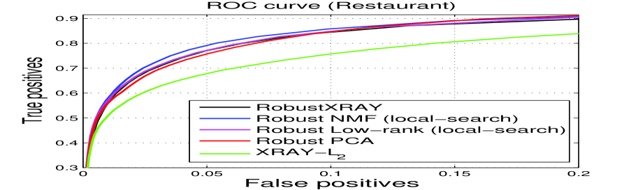
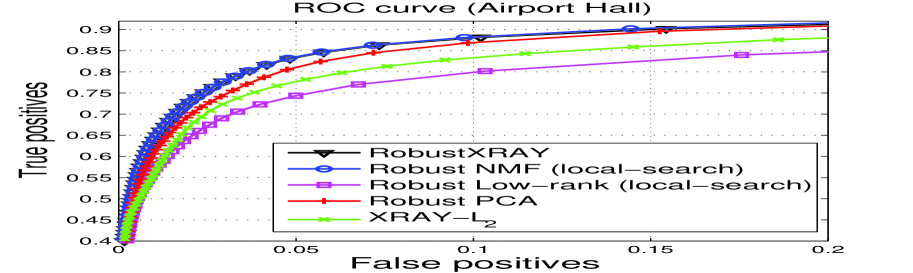
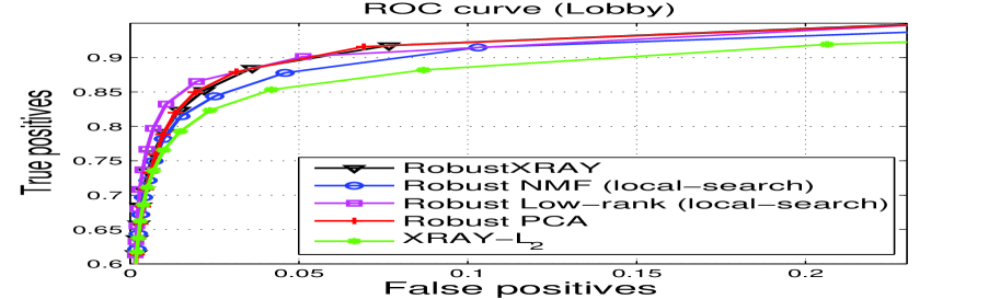
Figure 5: Foreground-background separation: ROC curves with various methods for Restaurant, Airport Hall and Lobby video sequences. The ranges for X and Y axes are chosen to better highlight the differences among the ROC curves. (best viewed in color)

5.3 Foreground-background Separation

In this section, we consider the problem of foreground-background separation in video. The camera position is assumed to be almost fixed throughout the video. In all video frames, the camera captures the background scene superimposed with a limited foreground activity (e.g., movement of people or objects). Background is assumed to be stationary or slowly varying across frames (variations in illumination and shadows due to lighting or time of day) while foreground is assumed to be composed of objects that move across frames but span only a few pixels. If we vectorize all video frames and stack them as rows to form the matrix $\mathbf{X}$, the foreground-background separation problem can be modeled as decomposing $\mathbf{X}$ into a low-rank matrix $\mathbf{L}$ (modeling the background) and a sparse matrix $\mathbf{S}$ (modeling the foreground).

Connection to Median Filtering: Median filtering is one of the most commonly used background modeling techniques Sen-Ching & Kamath (2004), which simply models the background as the pixel-wise median of the video frames. The assumption is that each pixel location stays in the background for more than half of the video frames. Consider the NMF of inner-dimension 1: $\min_{\bm{w}\geq 0,\bm{h}\geq 0}\|\mathbf{X}-\bm{w}\bm{h}\|_{1}$. If we constrain the vector $\bm{w}$ to be all ones, the solution $\bm{h}^{*}=\mathop{\rm arg\,min}_{\bm{w}=\mathbf{1},\bm{h}\geq 0}\|\mathbf{X}-\bm{w}\bm{h}\|_{1}$ is nothing but the element-wise median of all rows of $\mathbf{X}$. More generally, if $\bm{w}$ is constrained to be such that $\bm{w}_{i}=c>0$ $\forall$ $i$, the solution $\bm{h}^{*}$ is a scaled version of the element-wise median vector. Hence Robust NMF under this very restrictive setting is equivalent to median filtering on the video frames, and we can hope that loosening this assumption and allowing for higher inner-dimension in the factorization can help in modeling more variations in the background.

We use three video sequences for evaluation: Restaurant, Airport Hall and Lobby Li et al. (2004). Restaurant and Airport Hall are videos taken at a buffet restaurant and at a hall of an airport, respectively. The lighting are distributed from the ceilings and significant shadows of moving persons cast on the ground surfaces from different directions can be observed in the videos. Lobby video sequence was captured from a lobby in an office building and has background changes due to lights being switched on/off. The ground truth (whether a pixel belongs to foreground or background) is also available for these video sequences and we use it to generate the ROC curves. We mainly compare RobustXray  with Robust PCA which is widely considered state of the art methodology for this task in the Computer Vision community. In addition, we also compare with two local-search based approaches: (i) Robust NMF (local-search) which solves $\min_{\mathbf{W}\geq 0,\mathbf{H}\geq 0}\|\mathbf{X}-\mathbf{W}\mathbf{H}\|_{1}$ using local search, and (ii) Robust Low-rank (local-search) which solves $\min_{\mathbf{W},\mathbf{H}}\|\mathbf{X}-\mathbf{W}\mathbf{H}\|_{1}$ using local search. We use an ADMM based optimization procedure for both these local-search methods. We also show results with Xray-$\ell_{2}$ of Kumar et al. (2013) to highlight the importance of having near-separable NMFs with $\ell_{1}$ loss for this problem. For both Xray-$\ell_{2}$ and RobustXray , we do 1 to 2 refitting steps to refine the solution (i.e., solve $\mathbf{H}=\min_{\mathbf{B}\geq 0}\|\mathbf{X}-\mathbf{X}_{A}\mathbf{B}\|_{1}$ then solve $\mathbf{W}=\min_{\mathbf{C}\geq 0}\|\mathbf{X}-\mathbf{C}\mathbf{H}\|_{1}$). For all the methods, we do a grid search on the parameters (inner-dimension or rank parameter for the factorization methods and $\lambda$ parameter for Robust PCA) and report the best results for each method.

Fig. 5 shows the ROC plots for the three video datasets. For Restaurant data, all robust methods (those with $\ell_{1}$ penalty on the foreground) perform almost similarly. For Airport Hall data, RobustXray  is tied with local-search based Robust NMF and these two are better than other methods. Surprisingly, Xray-$\ell_{2}$ performs better than local-search based Robust Low-rank which might be due to bad initialization. For Lobby data, local-search based Robust low-rank, Robust PCA and RobustXray  perform almost similarly, and are better than local-search based Robust NMF. The results on these three datasets show that RobustXray  is a promising method for the problem of foreground-background separation which has a huge advantage over Robust PCA in terms of speed. Our MATLAB implementation was at least 10 times faster than the inexact Augmented Lagrange Multiplier (i-ALM) implementation of Lin et al. (2010).

6 Conclusion and Future Work

We have proposed generalized conical hull algorithms to extend near-separable NMFs to robust ($\ell_{1}$) loss function and Bregman divergences. Empirical results on exemplar selection and video background-foreground modeling problems suggest that this is a promising methodology. Avenues for future work include formal theoretical analysis of noise robustness and applications to online settings.

Appendix A Near-separable NMF with Bregman divergence

Let $A$ be the set of anchors selected so far by the algorithm. Let $\phi(\cdot)$ be the strictly convex function that induces the Bregman divergence $D_{\phi}(x,y)=\phi(x)-\phi(y)-\phi^{\prime}(y)(x-y)$. For two matrices $\mathbf{X}$ and $\mathbf{Y}$, we consider the Bregman divergence of the form $D_{\phi}(\mathbf{X},\mathbf{Y}):=\sum_{ij}D_{\phi}(\mathbf{X}_{ij},\mathbf{Y}_{ij})$. We make the following assumptions for the proofs in this section which are satisfied by almost all the Bregman divergences of interest:

Assumption 1: The first derivative of $\phi$, $\phi^{\prime}$, is smooth.

Assumption 2: The second derivative of $\phi$, $\phi^{\prime\prime}$, is positive at all nonzero points, i.e., $\phi^{\prime\prime}(x)>0$ for $x\neq 0$. Note that strict convexity does not necessarily imply $\phi^{\prime\prime}(x)>0$ for all $x$ while the converse is true.

Here we consider the projection step

$$\mathbf{H}=\mathop{\rm arg\,min}_{\mathbf{B}\geq 0}D_{\phi}(\mathbf{X},\mathbf{X}_{A}\mathbf{B}),$$ (6)

and the following selection criteria to identify the next anchor column:

$$j^{\star}=\mathop{\rm arg\,max}_{j}\frac{(\phi^{\prime\prime}(\mathbf{X}_{A}\mathbf{H}_{i})\odot\mathbf{R}_{i})^{T}\mathbf{X}_{j}}{\mathbf{p}^{T}\mathbf{X}_{j}}$$ (7)

for any $i:\|\mathbf{R}_{i}\|>0$, where $\mathbf{R}=\mathbf{X}-\mathbf{X}_{A}\mathbf{H}$ and $\phi^{\prime\prime}(\mathbf{x})$ is the vector of second derivatives of $\phi(\cdot)$ evaluated at individual elements of the vector $\mathbf{x}$ (i.e., $[\phi^{\prime\prime}(\mathbf{x})]_{j}=\phi^{\prime\prime}(\mathbf{x}_{j})$), $\mathbf{p}$ is any strictly positive vector not collinear with $(\phi^{\prime\prime}(\mathbf{X}_{A}\mathbf{H}_{i})\odot\mathbf{R}_{i})$, and $\odot$ denotes element-wise product of vectors. For a matrix $\mathbf{X}$, $\mathbf{X}_{ij}$ denotes $ij$th element, $\mathbf{X}_{i}$ denotes $i$th column and $\mathbf{X}_{A}$ denotes the columns of $\mathbf{X}$ indexed by set $A$. $\mathbf{X}_{A_{ij}}$ denotes $ij$th column of matrix $\mathbf{X}_{A}$.

Here we show the following result regarding the anchor selection property of Eq. 7. Recall that an anchor is a column that can not be expressed as conic combination of other columns in $\mathbf{X}$.

Theorem A.1.

If the maximizer of Eq. 7 is unique, the data point $\mathbf{X}_{j^{\star}}$ added at each iteration in the Selection step, is an anchor that has not been selected in one of the previous iterations.

The proof of this theorem follows the same style as the proof of Theorem $3.1$ in the main paper. We need the following lemmas to prove Theorem A.1.

Lemma A.1.

Let $\mathbf{R}$ be the residual matrix obtained after Bregman projection of columns of $\mathbf{X}$ onto the current cone. Then, $(\phi^{\prime\prime}(\mathbf{X}_{A}\mathbf{H})\odot\mathbf{R})^{T}\mathbf{X}_{A}\leq 0$, where $\mathbf{X}_{A}$ are anchor columns selected so far by the algorithm.

Proof.

Residuals are given by $\mathbf{R}=\mathbf{X}-\mathbf{X}_{A}\mathbf{H}$, where $\mathbf{H}=\mathop{\rm arg\,min}_{\mathbf{B}\geq 0}D_{\phi}(\mathbf{X},\mathbf{X}_{A}\mathbf{B})$.
Forming the Lagrangian for Eq. 6, we get $\mathcal{L}(\mathbf{B},\bm{\Lambda})=D_{\phi}(\mathbf{X},\mathbf{X}_{A}\mathbf{B})-tr(\bm{\Lambda}^{T}\mathbf{B})$, where the matrix $\bm{\Lambda}$ contains the non-negative Lagrange multipliers.

At the optimum $\mathbf{B}=\mathbf{H}$, we have $\nabla\mathcal{L}=0$ which means

$$~{}~{}~{}~{}~{}~{}\frac{\partial}{\partial\mathbf{B}_{mn}}\biggl{.}D_{\phi}(\mathbf{X},\mathbf{X}\mathbf{B})\biggr{|}_{\mathbf{B}=\mathbf{H}}=\bm{\Lambda}_{mn}$$

$$\Rightarrow\sum_{i}\biggl{[}-\mathbf{X}_{A_{im}}\phi^{\prime}((\mathbf{X}_{A}\mathbf{H})_{in})-\mathbf{X}_{A_{im}}\phi^{\prime\prime}((\mathbf{X}_{A}\mathbf{H})_{in})(\mathbf{X}_{in}\biggr{.}$$

$$-\biggl{.}(\mathbf{X}_{A}\mathbf{H})_{in})+\phi^{\prime}((\mathbf{X}_{A}\mathbf{H})_{in})\mathbf{X}_{A_{im}}\biggr{]}=\bm{\Lambda}_{mn}$$

$$\Rightarrow\sum_{i}-\biggl{[}\mathbf{X}_{A_{im}}\phi^{\prime\prime}((\mathbf{X}_{A}\mathbf{H})_{in})(\mathbf{X}_{in}-(\mathbf{X}_{A}\mathbf{H})_{in})\biggr{]}=\bm{\Lambda}_{mn}$$

$$\Rightarrow\left[\phi^{\prime\prime}(\mathbf{X}_{A}\mathbf{H})\odot(\mathbf{X}-\mathbf{X}_{A}\mathbf{H})\right]_{n}^{T}\mathbf{X}_{A_{m}}=-\bm{\Lambda}_{mn}$$

$$\Rightarrow\left[\phi^{\prime\prime}(\mathbf{X}_{A}\mathbf{H})\odot(\mathbf{X}-\mathbf{X}_{A}\mathbf{H})\right]^{T}\mathbf{X}_{A}=-\bm{\Lambda}^{T}\leq 0,$$

where $\phi^{\prime\prime}(\cdot)$ is the second derivative of $\phi(\cdot)$ that operates element-wise on the argument (vector or matrix). ∎

Lemma A.2.

For any point $\mathbf{X}_{i}$ exterior to the current cone, we have $(\phi^{\prime\prime}(\mathbf{X}_{A}\mathbf{H})\odot\mathbf{R})_{i}^{T}\mathbf{X}_{i}>0$.

Proof.

For a vector $\mathbf{v}>0$ and any vector $\bm{z}$, we have $(\mathbf{v}\odot\bm{z})^{T}\bm{z}=\sum_{i}\mathbf{v}_{i}\bm{z}_{i}^{2}>0$. Taking $\mathbf{v}$ to be $\phi^{\prime\prime}(\mathbf{X}_{A}\mathbf{H}_{i})$ and $\bm{z}$ to be $\mathbf{R}_{i}$, we have

$$\begin{split}&(\phi^{\prime\prime}(\mathbf{X}_{A}\mathbf{H}_{i})\odot\mathbf{R}_{i})^{T}\mathbf{R}_{i}>0\\ &\Rightarrow(\phi^{\prime\prime}(\mathbf{X}_{A}\mathbf{H}_{i})\odot\mathbf{R}_{i})^{T}(\mathbf{X}_{i}-\mathbf{X}_{A}\mathbf{H}_{i})>0\end{split}$$ (8)

By complementary slackness condition at the optimum, we have $\bm{\Lambda}_{ji}\mathbf{H}_{ji}=0$. From the KKT condition in the proof of previous lemma, we have $\left[\phi^{\prime\prime}(\mathbf{X}_{A}\mathbf{H}_{i})\odot\mathbf{R}_{i}\right]^{T}\mathbf{X}_{A}=-\bm{\Lambda}_{i}^{T}$. Hence

$\left[\phi^{\prime\prime}(\mathbf{X}_{A}\mathbf{H}_{i})\odot\mathbf{R}_{i}\right]^{T}\mathbf{X}_{A}\mathbf{H}_{i}=-\bm{\Lambda}_{i}^{T}\mathbf{H}_{i}=0$.

Hence Eq 8 reduces to

$(\phi^{\prime\prime}(\mathbf{X}_{A}\mathbf{H}_{i})\odot\mathbf{R}_{i})^{T}\mathbf{X}_{i}>0$. ∎

Using the above two lemmas, we can prove Theorem A.1 as follows.

Proof.

Denoting $\mathbf{D}_{i}^{\star}:=(\phi^{\prime\prime}(\mathbf{X}_{A}\mathbf{H}_{i})\odot\mathbf{R}_{i})$ in the proof of Theorem 3.1 of the main paper, all the statements of the proof directly apply in the light of Lemma A.1 and Lemma A.2. ∎

References

- Arora et al. (2012) Arora, Sanjeev, Ge, Rong, Kannan, Ravi, and Moitra, Ankur. Computing a nonnegative matrix factorization – provably. In STOC, 2012.
- Arora et al. (2013) Arora, Sanjeev, Ge, Rong, Halpern, Yoni, Mimno, David, Moitra, Ankur, Sontag, David, Wu, Yichen, and Zhu, Michael. A practical algorithm for topic modeling with provable guarantees. 2013.
- Banerjee et al. (2005) Banerjee, Arindam, Merugu, Srujana, Dhillon, Inderjit S, and Ghosh, Joydeep. Clustering with bregman divergences. Journal of Machine Learning Research, 6:1705–1749, 2005.
- Bittorf et al. (2012) Bittorf, Victor, Recht, Benjamin, Re, Christopher, and Tropp, Joel A. Factoring nonnegative matrices with linear programs. In NIPS, 2012.
- Boyd et al. (2011) Boyd, Stephen, Parikh, Neal, Chu, Eric, Peleato, Borja, and Eckstein, Jonathan. Distributed optimization and statistical learning via the alternating direction method of multipliers. Foundations and Trends® in Machine Learning, 3(1):1–122, 2011.
- Cichocki et al. (2009) Cichocki, A., Zdunek, R., Phan, A. H., and Amari, S. Non-negative Matrix and Tensor Factorizations. Wiley, 2009.
- Clarkson (1994) Clarkson, K. More output-sensitive geometric algorithms. In FOCS, 1994.
- Donoho & Stodden (2003) Donoho, D. and Stodden, V. When does non-negative matrix factorization give a correct decomposition into parts? In NIPS, 2003.
- Dula et al. (1998) Dula, J. H., Hegalson, R. V., and Venugopal, N. An algorithm for identifying the frame of a pointed finite conical hull. INFORMS Jour. on Comp., 10(3):323–330, 1998.
- Elhamifar et al. (2012) Elhamifar, Ehsan, Sapiro, Guillermo, and Vidal, Rene. See all by looking at a few: Sparse modeling for finding representative objects. In CVPR, 2012.
- Esser et al. (2012) Esser, Ernie, M ller, Michael, Osher, Stanley, Sapiro, Guillermo, and Xin, Jack. A convex model for non-negative matrix factorization and dimensionality reduction on physical space. IEEE Transactions on Image Processing, 21(10):3239 – 3252, 2012.
- Fan et al. (2008) Fan, R.-E., Chang, K.-W., Hsieh, C.-J., Wang, X.-R., and Lin, C.-J. Liblinear: A library for large linear classification. JMLR, 2008.
- Févotte et al. (2009) Févotte, Cédric, Bertin, Nancy, and Durrieu, Jean-Louis. Nonnegative matrix factorization with the itakura-saito divergence: With application to music analysis. Neural computation, 21(3):793–830, 2009.
- Gillis & Vavasis (2012) Gillis, Nicolas and Vavasis, Stephen A. Fast and robust recursive algorithms for separable nonnegative matrix factorization. arXiv:1208.1237v2, 2012.
- Greene & Cunningham (2006) Greene, Derek and Cunningham, Pádraig. Practical solutions to the problem of diagonal dominance in kernel document clustering. In ICML, 2006.
- Guan et al. (2012) Guan, Naiyang, Tao, Dacheng, Luo, Zhigang, and Shawe-Taylor, John. Mahnmf: Manhattan non-negative matrix factorization. CoRR abs/1207.3438, 2012.
- Hsieh & Dhillon (2011) Hsieh, C. J. and Dhillon, I. S. Fast coordinate descent methods with variable selection for non-negative matrix factorization. In KDD, 2011.
- Kim & Park (2007) Kim, Hyunsoo and Park, Haesun. Sparse non-negative matrix factorizations via alternating non-negativity-constrained least squares for microarray data analysis. Bioinformatics, 23:1495–1502, 2007.
- Kumar et al. (2013) Kumar, Abhishek, Sindhwani, Vikas, and Kambadur, Prabhanjan. Fast conical hull algorithms for near-separable non-negative matrix factorization. In ICML, 2013.
- Lee & Seung (1999) Lee, D. and Seung, S. Learning the parts of objects by non-negative matrix factorization. Nature, 401(6755):788–791, 1999.
- Li et al. (2012) Li, Liangda, Lebanon, Guy, and Park, Haesun. Fast bregman divergence nmf using taylor expansion and coordinate descent. In KDD, 2012.
- Li et al. (2004) Li, Liyuan, Huang, Weimin, Gu, Irene Yu-Hua, and Tian, Qi. Statistical modeling of complex backgrounds for foreground object detection. Image Processing, IEEE Transactions on, 13(11):1459–1472, 2004.
- Lin (2007) Lin, C.-J. Projected gradient methods for non-negative matrix factorization. Neural Computation, 2007.
- Lin et al. (2010) Lin, Zhouchen, Chen, Minming, and Ma, Yi. The augmented lagrange multiplier method for exact recovery of corrupted low-rank matrices. arXiv preprint arXiv:1009.5055, 2010.
- (25) Reuters. archive.ics.uci.edu/ml/datasets/Reuters-21578+Text+Categorization+Collection.
- Sen-Ching & Kamath (2004) Sen-Ching, S Cheung and Kamath, Chandrika. Robust techniques for background subtraction in urban traffic video. In Electronic Imaging 2004, pp. 881–892, 2004.
- Sra & Dhillon (2005) Sra, Suvrit and Dhillon, Inderjit S. Generalized nonnegative matrix approximations with bregman divergences. In Advances in neural information processing systems, pp. 283–290, 2005.