Spatially embedded growing small-world networks

Abstract

Networks in nature are often formed within a spatial domain in a dynamical manner, gaining links and nodes as they develop over time. We propose a class of spatially-based growing network models and investigate the relationship between the resulting statistical network properties and the dimension and topology of the space in which the networks are embedded. In particular, we consider models in which nodes are placed one by one in random locations in space, with each such placement followed by configuration relaxation toward uniform node density, and connection of the new node with spatially nearby nodes. We find that such growth processes naturally result in networks with small-world features, including a short characteristic path length and nonzero clustering. These properties do not appear to depend strongly on the topology of the embedding space, but do depend strongly on its dimension; higher-dimensional spaces result in shorter path lengths but less clustering.

I Introduction

One fascinating property of many real-world networks is that they are often “small worlds” in the sense that they have both short average path length and high clustering Milgram (1967); Watts and Strogatz (1998); Newman (2003). The shortest path length between two nodes is the smallest number of links in the path connecting that pair of nodes, and the average path length is the average of this value over all node pairs in the network. It is regarded as short if it grows very slowly with network size. To quantify the clustering of an undirected network, we use the clustering coefficient, which is defined as three times the number of triangles in the network divided by the number of link pairs that share a common node Newman (2009). In networks with high clustering, if two nodes are both neighbors of a third node, they are also likely to be connected to one another. A variety of real-world networks, from social networks to neuronal networks, exhibit the small-world property, and this has fundamental consequences for dynamical processes such as spread of information or disease Watts and Strogatz (1998).

Networks with spatial constraints typically have geographically short-range edges, and it is thus relevant that both the original Watts-Strogatz small-world model Watts and Strogatz (1998) and many real networks with the small-world property are embedded in physical space. For example, the Internet, a network of routers connected via cables, is essentially embedded on the two-dimensional surface of the Earth and tends to have mostly local links, presumably due to the cost of wiring Lakhina et al. (2003). This has led many researchers to consider network models with spatial embedding Ozik et al. (2004); Przulj et al. (2010); Herrmann et al. (2003); Bullock et al. (2010); Guan and Wu (2008); Zhang et al. (2006, 2007); Bassett et al. (2010); Barthélemy (2003); Vázquez et al. (2002). Work on this topic has revealed that small-world properties are found in a variety of spatially embedded networks, including networks of neurons, power grids, and social interactions Watts and Strogatz (1998); Smith Bassett and Bullmore (2006).

Two other key aspects of many real-world networks are that they grow with time (new nodes are added), and that nodes may move in space. For example, new people may join social networks with time, and friendships typically form between people who live near one another, but people may also move to new locations. Although some studies have considered dynamically growing networks, they frequently assume that nodes remain fixed in their initial positions Bullock et al. (2010); Guan and Wu (2008); Przulj et al. (2010) or consider growing networks which are not embedded in space Davidsen et al. (2002); Callaway et al. (2001).

In Ref. Ozik et al. (2004), Ozik et al. considered a model which incorporates both a growing number of nodes and node movement. In this model, nodes are placed randomly on the circumference of a circle, but undergo small displacements to maintain a constant density over time. Each node initially forms links only to its geographic neighbors, but, due to growth, these links can subsequently be stretched in length, becoming long-range. Due to the emergence of these long-range links, this model also generates networks with the small-world property, but in this case it is a consequence of the growth process, rather than the spontaneous formation of long-range edges. However, since the physical properties of typical spatial systems typically depend on the dimension of the embedding space, the main limitation of Ref. Ozik et al. (2004) is that only a one-dimensional space (the circle) is treated. Thus, in this paper, we generalize the model of Ozik et al. (2004) by introducing and analyzing a class of growing undirected network models that have spatially constrained nodes able to move about in an embedding space of arbitrary dimension. (We note that, for real applications, dimensions two and three are commonly most relevant.)

II The Circle Network Model

In Ref. Ozik et al. (2004), the authors presented a model, henceforth referred to as the Circle Network Model, which considers an undirected network which initially has $m+1$ uniformly separated, all-to-all connected nodes on the circumference of a circle. At each discrete growth step the network is grown according to the following rules:

1. A new node is placed at a randomly selected point on the circumference of the circle.

2. The new node is linked to its $m$ nearest neighbors ($m$ is even in Ref. Ozik et al. (2004)).

3. Preserving node positional ordering, the nodes are repositioned to make the nearest-neighbor distances uniform.

4. Steps (1-3) are repeated until the network has $N$ nodes.

It has been shown that this growth model leads to a small-world network with an exponentially decaying degree distribution Ozik et al. (2004). The original goal of the circle network model was to explore the effect that local geographic attachment has on the growth of networks and was partially motivated by the growth of biological (e.g., neuronal) networks as an organism develops from an embryo. In the present paper, we extend this analysis by considering networks growing by geographic attachment preference in more general spaces.

We define a network growth procedure to yield the small-world property if, as $N\to\infty$, (i) the average degree $\langle k\rangle$ of a node approaches a finite value; (ii) the characteristic graph path length $\ell$, the average value of the smallest number of links in a path joining a pair of randomly chosen nodes, does not grow with $N$ faster than $\log N$, as in an Erdős-Rényi random network Newman et al. (2001); Newman (2009); and (iii) the clustering coefficient $C$, the fraction of connected network triples which are also triangles, approaches a nonzero constant with increasing $N$ . The circle network model exhibits all three properties.

Degree distribution: The degree distribution $H(k)$ is the probability that a randomly selected node has $k$ network connections. For large $N$, the degree distribution of the circle network model approaches

$$H(k)=\frac{1}{m+1}\left(\frac{m}{m+1}\right)^{k-m}$$ (1)

for $k\geq m$, and $H(k)=0$ for $k<m$ Ozik et al. (2004). Since the number of new links added each time a new node is added is $m$, Eq. (1) yields the result that the average node degree $\langle k\rangle$ is $2m$, satisfying the criterion (i) for the small-world property.

Characteristic path length: In the circle network model, simulation results show that $\ell\sim\log N$, satisfying criterion (ii). This may be explained intuitively by noting that as new nodes are added, they push apart the older connected nodes, lengthening the spatial distance traversed by older edges. These older nodes can then have geographically long links, thus dramatically decreasing the shortest graph path length between any given pair of nodes.

Clustering coefficient: For the circle network model, it was shown that the clustering coefficient approaches a constant, positive, $m$-dependent value as $N\to\infty$, satisfying criterion (iii).

III Generalizing the Circle Network Model

Like the Watts-Strogatz model, the circle network model may be described as a one-dimensional ring model in which connections are initially formed with $m$ nearest neighbors. However, in the circle network model, long-distance edges do not form spontaneously, but are a natural result of the dynamics of network growth. Moreover, the circle network model naturally raises the question of whether networks grown in higher-dimensional spaces exhibit similar properties. A primary goal of this article is to address this question.

In what follows, we introduce two models that generalize the model of Ref. Ozik et al. (2004) to higher dimensionality (Secs. IV and V), and then present our results from analysis of these models (Secs. VI and VII). Our main results are as follows.

1. The coupling of network growth with local geographical attachment leads to small-world networks independent of the dimension of the underlying space.

2. The nodal degree distribution (Fig. 1) and age-degree relationship (Fig. 2) are independent of dimension as in ($i$).

3. The path length $\ell$ scales as $\log N$ with a coefficient that decreases with dimension (Fig. 3) for fixed average degree.

4. The clustering coefficient $C$ approaches a finite asymptotic value with increasing $N$ (Fig. 4) and this asymptotic value decreases with increasing dimension $d$ of the embedding space.

5. All of our results above appear to be independent of the global topology of the embedding space.

IV The Sphere Network Model

One natural generalization of embedding nodes on the one-dimensional circumference of a circle is to embed them on the two-dimensional surface of a sphere, or more generally on the $d$-dimensional surface of a hypersphere. The case $d=1$ corresponds to the circle network model. However, although it is trivial to arrange $N$ points along the circumference of a circle with uniform spacing, the analogous procedure is less well-defined on higher dimensional surfaces. One way to generalize the arrangement procedure is to consider nodes to act like point charges and to move them to a minimum electrostatic energy equilibrium configuration. The problem of finding the equilibrium configuration of point charges on the surface of a sphere dates back to 1904 when J. J. Thomson introduced his model of the atom, and the problem of obtaining such an equilibrium is sometimes referred to as the “Thomson problem” Thomson (1904). A related “generalized Thomson problem” assumes that the force between “charges” is proportional to $r^{-\alpha}$, where $r$ is the distance between charges, with $\alpha$ not necessarily equal to the Coulomb value, $\alpha=d$ Bowick et al. (2002). For reasons discussed in Sec. V, we use the value $\alpha=d-1$ in simulations.

Using the generalized Thomson problem as a guide, we develop a generalization of the circle network model, which we call the Sphere Network Model, as follows. We model the nodes as point charges confined to a unit spherical surface of dimension $d$. We successively add a new node onto the surface at random with uniform probability density per unit area and then add links to connect it to its $m$ nearest neighbors, where distance is defined as the shortest great circle path along the surface of the sphere between two nodes. Next we relax the node positions to minimize the potential energy of the configuration using a gradient descent procedure,

$$\frac{\text{d}\bm{x}_{i}}{\text{d}t} =P[\bm{F}_{i}],$$ (2)

$$\bm{F}_{i} =\sum_{j\neq i}\frac{\phantom{|}\bm{x}_{i}-\bm{x}_{j}\phantom{|^{d}}}{|\bm{x}_{i}-\bm{x}_{j}|^{d}},$$ (3)

where $\bm{x}_{i}$ is the $(d+1)$ dimensional position vector of node $i$, $|\bm{x}_{i}|=1$ for all $i$, and $P[\cdot]$ denotes projection onto the $d$-dimensional surface of the sphere. We note that, as new nodes are added, this procedure tends to yield a local energy minimum, as opposed to the global minimum (for some applications, such as modeling biological network growth, the identification of local rather global minima might be viewed as more appropriate.) Note that, for large $N$, the repulsive interaction ensures that the points are distributed approximately uniformly on the surface of the sphere.

V The Plum Pudding Network Model

The sphere network model described above has the topological feature that the geographical embedding region does not have any boundary, which allows us to find a nearly-uniform distribution of nodes by imagining them to be identical charges with repulsive interactions. We have also tested another model with a different topology having a boundary and using a different mechanism to encourage uniform distribution of nodes. We call this second model the Plum Pudding Network Model after Thomson’s famous model of the atom Thomson (1904).

We again model our nodes as a collection of negative point charges in $d$ dimensions. The growth procedure is similar to the previous models; we place new nodes randomly in our volume and connect them to their $m$ nearest neighbors, where here we define nearest to be the Euclidean distance between the nodes. Now, however, we regard the nodes as free to move in a unit radius, $d$-dimensional ball. (For $d=1$, the unit ball is the interval $-1\leq x\leq 1$; for $d=2$, it is the region enclosed by the unit circle.) We assume that the ball contains a uniform background positive charge density such that the total background charge in the sphere is equal and opposite to that of the $N$ network nodes. As in the sphere model, after adding a node with uniform probability density within the unit $d$-dimensional ball, we relax the charge configuration to a local energy minimum. Here, the relaxation is described by

$$\frac{\text{d}\bm{x}_{i}}{\text{d}t}=\bm{F}_{i}-N\bm{x}_{i}$$ (4)

where $\bm{x}_{i}$ is a $d$-dimensional position vector with respect to the center of the ball, $\bm{F}_{i}$ is as in Eq. (3), and the term $N\bm{x}_{i}$ is due to the positive charge density.

Note that, in order to apply Gauss’s law for the background charge, we have assumed a force law proportional to $r^{-(d-1)}$. Gauss’s law, in turn, implies that when $N$ is large, the nodes will be approximately uniformly distributed in the ball in order to cancel the uniform positive background charge. Although any repulsive force law can, in principle, be used for the sphere model, we chose to use the same force law in Sec. IV in order to facilitate comparisons of the results between the two models.

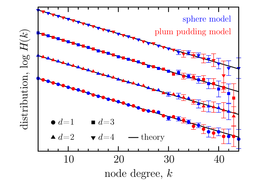
Figure 1: The logarithm of the degree distribution, $\log(H(k))$, versus degree $k$, for the sphere network model (blue markers) and the plum pudding model (red markers), using $N=10^{4}$ and $m=4$. Data are shown for $d=1$ (circles), $d=2$ (triangles), $d=3$ (squares), and $d=4$ (inverted triangles). Since all four cases have nearly identical results, an arbitrary linear offset has been used to separate data for visualization. Error bars are shown when they exceed the point size. Solid black lines correspond to the theoretical prediction of Eq. (1).

VI Degree Distribution

The distribution of node degrees can be derived analytically, does not depend on dimension, and is the same for the sphere and plum pudding models. This can be derived from the fact that, for large $N$, the probability that a newly added node will form an edge to any particular existing node is $m/N$ for all nodes. This is because existing nodes are distributed approximately uniformly, and new nodes are placed randomly according to a uniform probability distribution. Here we show that for each considered model, we produce the same master equation governing the evolution of the degree distribution as that found for the circle model in Ozik et al. (2004). This master equation is not specific to the spatial structure of the network and appears, in various forms, in other network models, such as the Deterministic Uniform Random Tree of Ref. Zhang et al. (2008).

We define $\hat{G}(k,N)$ to be the number of nodes with degree $k$ at growth step $N$ (i.e., when the system has $N$ nodes). When a node is added to the network it is initially connected to its $m$ nearest neighbors, so upon creation, $k=m$ for each node, meaning that $\hat{G}(k,N)=0$ for $k<m$. Since each existing node is equally likely to be chosen to be connected to the new node, there is an $m/N$ probability that any given node will have its degree incremented by 1. Averaging $\hat{G}(k,N)$ over all possible random node placements, we obtain a master equation for the evolution of $G(k,N)$, the average of $\hat{G}(k,N)$ over all possible randomly grown networks,

$$\begin{split}G(k,N+1)=G(k,N)&-\frac{m}{N}G(k,N)\\ &+\frac{m}{N}G(k-1,N)+\delta_{km},\end{split}$$ (5)

where $\delta_{km}$ is the Kronecker delta function. The first term on the right is the expected number of nodes with degree $k$ at growth step $N$. The second term is the expected number of nodes with degree $k$ at growth step $N$ that are promoted to degree $k+1$. The third term is the expected number of nodes with degree $k-1$ at growth step $N$ that are promoted to degree $k$. The last term on the right is the new node with degree $m$.

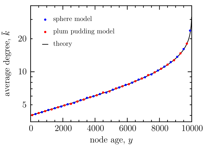
Figure 2: The mean degree $\bar{k}(y,N)$ of a node of age $y$ in a network with $N$ nodes on semilogarithmic axes. Data are shown for the sphere network model (blue) and plum pudding model (red), both with $d=2$, $m=4$, and $N=10^{4}$. Errors are smaller than the point size. The solid black line is the theoretical prediction given by Eq. (6).

It was shown by Ozik et al. Ozik et al. (2004) that this master equation leads to an exponentially decaying degree distribution with an asymptotically $N$ invariant form $H(k)=\lim_{N\to\infty}G(k,N)/N$ given by Eq. (1) for $k\geq m$ and $H(k)=0$ for $k<m$. Interestingly, this degree distribution comes only from the growth process and the uniform probability of attaching new links to existing nodes. As seen in Fig. 1, for $m=4$, $N=10^{4}$, with $d=1$, $2$, $3$, or $4$, Eq. (1) is well satisfied by numerical simulations of both models.

Intuitively, we expect that older nodes in each model will accumulate more edges and become network hubs. The relationship between degree and age is also straightforward to investigate in this model. Here, we calculate an expression for the expected degree $\bar{k}(y,N)$ of a node that has existed for $y$ growth steps, given that the network size is $N$ ($y<N$). Each node connects to its $m$ nearest neighbors upon creation, and the probability of incrementing the degree of the node is $m/N$ when the size of the network is $N$. Thus we obtain

$$\begin{split}\bar{k}(y,N)&=m+m\sum_{n=N-y+1}^{N}\frac{1}{n}\\ &\approx m+m\log\frac{N}{N-y}+\mathcal{O}\left(\frac{1}{N^{2}}\right).\end{split}$$ (6)

Once again, since this derivation uses only the assumption that each node has an equal chance each growth step to have its degree incremented, the result holds for both of the models discussed here. This represents a specific example of the fact that in dynamically growing networks, older nodes are preferentially connected to subsequent nodes, as discussed in Ref. Callaway et al. (2001). Numerical simulations in Fig. 2 demonstrate that Eq. (6) is satisfied for both models. For simplicity, results are only presented for $d=2$, but Eq. (6) has no dependence on the embedding space, and thus holds for other dimensions as well.

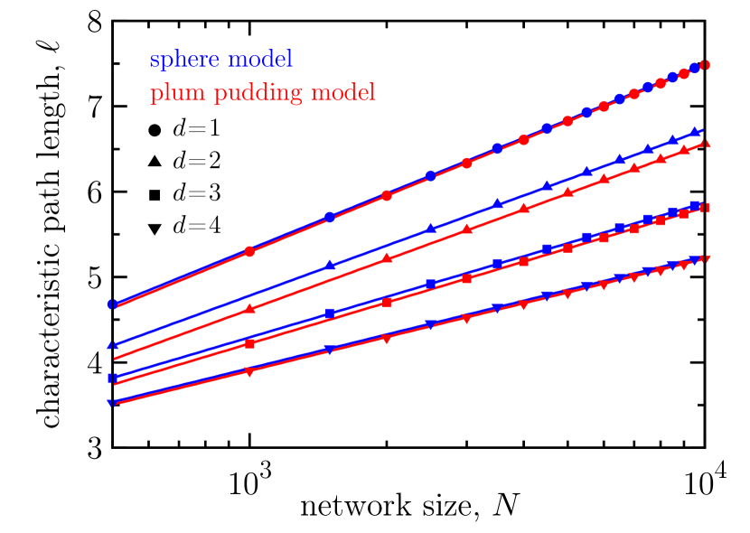
Figure 3: The characteristic graph path length ($\ell$) versus network size $N$ on semilogarithmic axes for the sphere model (blue markers) and the plum pudding model (red markers). The path length shows the desired scaling, $\ell\sim\log N$. Results are shown for $d=1$ (circles), $2$ (triangles), $3$ (squares), and $4$ (inverted triangles), all using $m=4$. Errors are smaller than the point size. In general, the average shortest path is shorter for higher dimensions $d$ in both models.

VII Path Length and Clustering Coefficient

For the sphere and plum pudding network models, we find numerically that the the average shortest path length $\ell$ scales logarithmically with the network size $N$, that is, $\ell\sim\log N$. See Fig. 3. The scaling $\ell\sim\log N$ is expected because as the network grows in size, the older nodes are pushed apart by the repulsive force, thus leaving bridges across the network that span a significant geographic distance. These long range links serve to connect spatially separated regions of highly interconnected nodes, dramatically reducing the shortest path length between any two nodes in the network. At each growth step only geographically local connections are made, but due to the dynamic nature of the nodes’ spatial positions, each growth step can make existing links longer in physical space, thus building bridges across the network.

We see from Fig. 3 that, for given values of $N$ and $m$, the characteristic path length decreases with $d$ and is shorter than that of the corresponding one-dimensional case (the original circle network model). One possible explanation for this is that in a higher dimensional space, it is easier to separate existing nodes by placing a new node, because nodes can move around one another, making it easier for short-range links to be stretched into shortcuts as the network grows. This is in contrast to the circle network model, in which each node is forever locked between its two original spatial neighbors until a new node is placed directly between them.

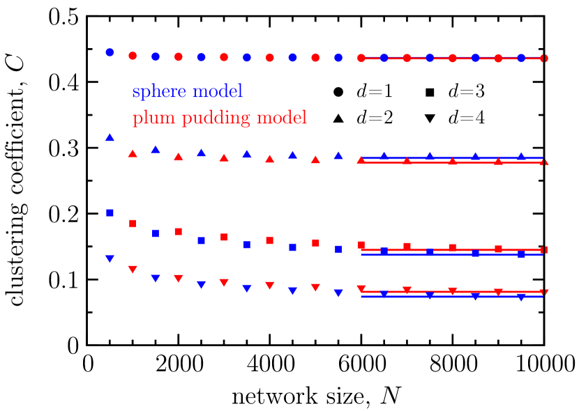
Figure 4: Clustering coefficient $C$ versus network size $N$ for the sphere network model (blue markers) and plum pudding model (red markers), both with $m=4$. Results are shown for $d=1$ (circles), $2$ (triangles), $3$ (squares), and $4$ (inverted triangles). Errors are smaller than the point size. Horizontal lines are drawn through the last data point in each series.

For both models, we also find that the clustering coefficient $C$ is nonzero for large $N$, but depends on the dimension of the embedding space. Results for the clustering coefficient $C$ versus the number of nodes $N$ with $d=1$, $2$, $3$, and $4$, using $m=4$, are displayed in Fig. 4. Horizontal lines are drawn through the last point in each series. For the values of $d$ shown, we see that as $N$ increases, there is an initial decrease of $C$ for $N<1,000$, but the $N$ variation appears to effectively cease with increasing $N$. These results are consistent with an $N\to\infty$ asymptotic value close to the value at $N=10,000$. Assuming this to be the case, values for the large-$N$ clustering in the sphere model are given as follows: for $d=1$, $C\approx 0.44$; for $d=2$, $C\approx 0.28$; for $d=3$, $C\approx 0.14$; and for $d=4$, $C\approx 0.07$. Values for the plum pudding model are similar. Higher dimensional cases that we have examined ($d=5$–$9$) follow the same pattern. More specifically, we find that for a given value of $m$, the clustering coefficient decays algebraically with dimension, $C\sim d^{-\beta_{m}}$. In Fig. 5, we show that $\beta_{4}=1.88$ for the sphere model, while for larger values of $m$ we find $\beta_{m}$ decreases, but remains positive.

Thus we find that that both the sphere and plum pudding network models lead to networks exhibiting the small-world property, and their behaviors are similar. Thus spatial topology does not appear to be of great importance to the properties of the resulting network. Node addition, local edge formation, and relaxation towards uniform density appear to be sufficient for the occurrence of the small-world property. On the other hand, although the degree distribution does not depend on dimension (Sec. VI), an important result is that other network properties such as the clustering coefficient show a relatively strong dependence on dimensionality (Figs. 3–5).

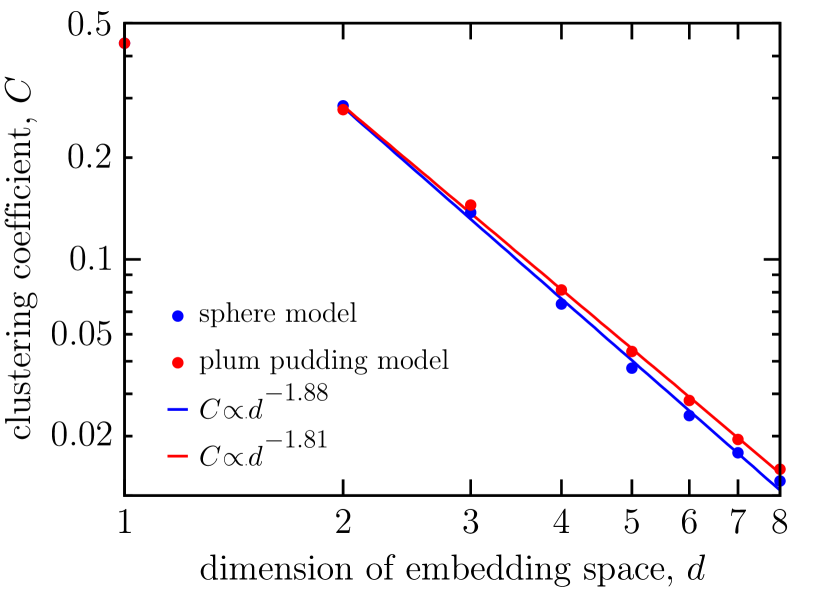
Figure 5: Asymptotic clustering coefficient $C$ versus dimension of embedding space $d$ for the sphere network model (blue) and plum pudding model (red) on logarithmic axes with $m=4$. Solid black lines are given by $C\propto d^{-\beta}$, $\beta$ was obtained from a least-squares fit to the data for $d\geq 2$. The resulting value of $\beta$ was $1.88$ for the sphere model and $1.81$ for the plum pudding model.

It is worth noting that the $d=1$ case of the plum pudding model does not reduce to the circle network model, but the two nonetheless show similar behavior, because they differ only at the boundary $x=\pm 1$. In both models, the relative spatial ordering of nodes is preserved, and the equilibrium case has perfectly uniform inter-nodal spacing, as opposed to models with $d\geq 2$, in which the concept of linear ordering is absent. In addition, when $d\geq 2$ in both the sphere and plum pudding models, exact, global regular-lattice positioning is not possible. For example, for $N\gg 1$ charges on a sphere with $d=2$, it is known that the equilibrium positioning on much of the area of the sphere is locally similar to a triangular lattice, but the sphere’s curvature leads to point and line defects in the lattice Bowick et al. (2002). Thus a natural question is whether the $d=1$ cases might have special properties in common that deviate from those for $d\geq 2$. It can be seen in Fig. 5 that one such property is that both $d=1$ cases do not follow the same scaling trend in clustering that we find for higher dimensions.

VIII Discussion

We have explored two models which generate networks with small-world features through local geographic attachment and growth, without direct formation of long-distance links. By allowing nodes to move in space, the initially formed local links can become long-range, thus providing a mechanism for how small-world networks can emerge from a growing collection of dynamically interacting and locally constrained vertices. Both models show similar behavior for the degree distribution, characteristic path length, and clustering coefficient. The qualitative similarity between the networks generated by the two models indicates that the small-world features are determined by geographic attachment and growth, not the topological features of the embedding space. However, the quantitative values of measures characterizing these features can depend on dimension; higher-dimensional spaces yield shorter path lengths but less clustering.

These findings may offer insight into the origin of small-world features in diverse growing networks, such as power grids and networks of neurons. In such systems, network growth may be an appropriate mechanism for the emergence of small-world features. We also speculate that similar ideas may explain the small-world property in some non-spatial networks, such as the world wide web, by replacing the physical space used in our model with a more abstract space of content (i.e., the location of a node represents the topic or purpose of a website, and websites link to other websites which have similar content).

We hope these findings will generate renewed interest in spatial networks with dynamically located nodes and in the role that growth plays in the development of important network features.

Acknowledgements: This work was supported by the National Science Foundation under grant number PHY-1156454 and by the Army Research Office under grant W911NF-12-1-0101.

References

- Milgram (1967) S. Milgram, Psych. Today 1, 61 (1967).
- Watts and Strogatz (1998) D. J. Watts and S. H. Strogatz, Nature 393, 440 (1998).
- Newman (2003) M. E. J. Newman, SIAM Rev. 45, 167 (2003).
- Newman (2009) M. E. J. Newman, Phys. Rev. Lett. 103, 058701 (2009).
- Lakhina et al. (2003) A. Lakhina, J. W. Byers, M. Crovella, and I. Matta, IEEE J. Sel. Areas Commun. 21, 934 (2003).
- Ozik et al. (2004) J. Ozik, B. R. Hunt, and E. Ott, Phys. Rev. E 69, 026108 (2004).
- Przulj et al. (2010) N. Przulj, O. Kuchaiev, A. Stevanovic, and W. Hayes, Pac. Symp. Biocomput., 2009, 178 (2010).
- Herrmann et al. (2003) C. Herrmann, M. Barthélemy, and P. Provero, Phys. Rev. E 68, 026128 (2003).
- Bullock et al. (2010) S. Bullock, L. Barnett, and E. A. Di Paolo, Complexity 16, 20 (2010).
- Guan and Wu (2008) Z.-H. Guan and Z.-P. Wu, Physica A 387, 314 (2008).
- Zhang et al. (2006) Z.-Z. Zhang, L.-L. Rong, and F. Comellas, J. Phys. A 39, 3253 (2006).
- Zhang et al. (2007) Z. Zhang, S. Zhou, Z. Shen, and J. Guan, Physica A 385, 765 (2007).
- Bassett et al. (2010) D. S. Bassett, D. L. Greenfield, A. Meyer-Lindenberg, D. R. Weinberger, S. W. Moore, and E. T. Bullmore, PLoS Comp. Biol. 6, e1000748 (2010).
- Barthélemy (2003) M. Barthélemy, Europhys. Lett. 63, 915 (2003).
- Vázquez et al. (2002) A. Vázquez, A. Flammini, A. Maritan, and A. Vespignani, ComPlexUs 1, 38 (2002).
- Smith Bassett and Bullmore (2006) D. Smith Bassett and E. Bullmore, Neuroscientist 12, 512 (2006).
- Davidsen et al. (2002) J. Davidsen, H. Ebel, and S. Bornholdt, Phys. Rev. Lett. 88, 128701 (2002).
- Callaway et al. (2001) D. S. Callaway, J. E. Hopcroft, J. M. Kleinberg, M. E. J. Newman, and S. H. Strogatz, Phys. Rev. E 64, 041902 (2001).
- Newman et al. (2001) M. E. J. Newman, S. H. Strogatz, and D. J. Watts, Phys. Rev. E 64, 026118 (2001).
- Note (1) In Ozik et al. (2004) an alternate definition of the clustering coefficient was used. Specifically, the local clustering of each node is , where is the number of links between the neighbors of node , and the global network clustering is the average of over .
- Thomson (1904) J. J. Thomson, Philos. Mag. 7, 237 (1904).
- Bowick et al. (2002) M. Bowick, A. Cacciuto, D. R. Nelson, and A. Travesset, Phys. Rev. Lett. 89, 185502 (2002).
- Zhang et al. (2008) Z. Zhang, S. Zhou, Y. Qi, and J. Guan, Eur. Phys. J. B 63, 507 (2008).