Critical percolation on mesoscopic triangulations

Abstract.

We extend Smirnov’s proof of the existence and conformal invariance of the scaling limit of critical site-percolation on the triangular lattice to particular sequences of periodic graphs with more arbitrary large-scale structure, obtained by piecing together triangular regions of the triangular lattice. While not formally speaking a scaling limit statement (as the graphs are not rescaled versions of each other), the result is a weak form of universality for critical percolation.

Introduction

The main goal of statistical physics is to understand the long-range properties of a model described by local, microscopic interactions. Typically, the model will be defined on a lattice and depend on a parameter (usually denoted by $\beta$ and interpreted as an inverse temperature) and exhibit a phase transition at a certain value $\beta_{c}$ of the parameter. This means that its qualitative behavior changes drastically between the high-temperature regime ($\beta<\beta_{c}$), where decorrelation between distant regions is observed, and the low-temperature regime ($\beta>\beta_{c}$) for which long-range ordering is present. The transition can often be characterized by the behavior of a correlation length which depends on the temperature and diverges at the critical point.

Such systems are most interesting when considered at their critical point. Indeed, the divergence of the correlation length indicates that if one can define a scaling limit when the mesh of the lattice is sent to $0$, such a limit should be non-trivial and invariant under scalings. In two dimensions, many scaling limits are moreover expected to be conformally invariant, i.e. invariant (or covariant) under the action of conformal maps. An archetypal example is that of Brownian motion, which is the scaling limit of simple random walk and is indeed conformally invariant in dimension two.

0.1. Percolation

There are very few models for which convergence to a scaling limit is known. The easiest to describe is (Bernoulli) percolation [4, 6]. It is described as follows: starting with the honeycomb lattice on the plane, color each face (each hexagon) black with probability $p\in(0,1)$ and white with probability $1-p$, independently of one another. One is then interested in the existence of unbounded chains of adjacent hexagons that are all colored black. It is not difficult to show that this is almost surely the case if $p$ is close enough to $1$, and almost surely not the case if it is small enough; there is a critical value $p_{c}$ separating the two possible behaviors. In this particular case, it is a result similar to Kesten’s celebrated theorem [5] that in fact $p_{c}=1/2$.

An equivalent way to see this model is to consider it as a random coloring of the vertices of the triangular lattice, which is dual to the honeycomb lattice. The model itself is therefore usually referred to as site percolation.

0.2. Cardy’s formula

It is one of the most striking recent results in the domain that critical site-percolation on the triangular lattice has a scaling limit. One precise statement of this uses crossing probabilities. Let $\Omega$ be a simply connected, bounded, smooth domain in the complex plane and let $(a,b,c,d)$ be a quadruple of boundary points of $\Omega$ — these data form a topological rectangle. Consider critical site-percolation on the intersection of $\Omega$ with the triangular lattice with mesh $\delta$.

Theorem 1 (Smirnov [11]).

Let $C_{\delta}(\Omega,a,b,c,d)$ be the event that there exists a chain of black vertices in $\Omega$, connecting the boundary arcs $ab$ and $cd$ — this is called a crossing event. Then,

1. As $\delta\to 0$, the probability of the event $C_{\delta}(\Omega,a,b,c,d)$ converges to a limit $\mathfrak{f}(\Omega,a,b,c,d)\in(0,1);$

2. Moreover, the limit is conformally invariant: if $\Phi:\Omega\to\Phi(\Omega)$ is a conformal map that extends continuously to the boundary of $\Omega$, then

   $$\mathfrak{f}(\Phi(\Omega),\Phi(a),\Phi(b),\Phi(c),\Phi(d))=\mathfrak{f}(\Omega,a,b,c,d).$$

The Riemann mapping theorem ensures that any such topological rectangle can be conformally mapped to a rectangle $\mathfrak{R}_{q}:=[0,q]\times[0,1]$, seen as a subset of the complex plane, in such a way that the boundary arcs $ab$ and $cd$ are sent to the vertical edges of $\mathfrak{R}_{q}$; the value of $q$ is prescribed by the topological rectangle. The limit $\mathfrak{f}$ can then be written in terms of $q$: there is a function $\mathfrak{C}:(0,+\infty)\to(0,1)$ satisfying

$$\mathfrak{f}(\Omega,a,b,c,d)=\mathfrak{f}(\mathfrak{R}_{q},q,q+i,i,0)=:\mathfrak{C}(q).$$

The existence and value of the function $\mathfrak{C}$ were first predicted by Cardy [3], and the value is known as Cardy’s formula.

As a consequence of this theorem, one gets the existence of a scaling limit for macroscopic percolation interfaces, described using SLE processes, from which one can then derive the existence of critical exponents: for instance [12], the probability that the origin is in an infinite component scales like $(p-p_{c})^{5/36+o(1)}$ as $p\downarrow p_{c}$, and the probability at the critical point that the cluster of the origin has radius at least $R$ behaves like $R^{-5/48+o(1)}$.

0.3. Universality

It is tempting to wonder how general the statement of Smirnov’s theorem really is. The qualitative features of percolation are the same in many two-dimensional lattices: there always is a non-trivial critical point, divergence of the correlation length, and in many cases uniform upper and lower bounds for crossing probabilities at the critical point (this is usually referred to as Russo-Seymour-Welsh theory [8, 9]).

Physicists expect more quantitative similarities: the conjecture of universality states that all Bernoulli percolation models on planar lattices will exhibit the same critical exponents and essentially the same scaling limit (even though the value of the critical point $p_{c}$ itself depends on the lattice). The question remains completely open from the mathematical point of view, and the triangular lattice is so far the only one on which a scaling limit is known to exist.

0.4. Statement of the results

The main result of the present paper is a partial universality statement, for mesoscopic triangulations i.e. triangulations of the plane with a local structure similar to the triangular lattice, but with a longer range one that is more arbitrary.

Let $\mathcal{T}$ be a periodic triangulation of the plane, embedded in the plane in a fixed way. Rescale $\mathcal{T}$ to have lattice mesh $\delta$, and replace each of its faces with a triangle of side length $N$ taken from the triangular lattice, welding such triangles along the edges of the initial triangulation. This produces a lattice $\mathcal{T}_{\delta,N}$, which has two characteristic lengths, $\delta$ and $\delta/N$. $\delta$ is understood to be small, but large with respect to the microscopic scale $\delta/N$, hence the name mesoscopic.

Theorem 2.

Assuming that $\mathcal{T}\!\!$ satisfies assumption 1 (see below), there exists a constant $c>0$ such that, as $\delta\to 0$ and $N\to\infty$ jointly, subject to the constraint $N>\delta^{-c}$, critical percolation on the mesoscopic lattice $\mathcal{T}_{\delta,N}$ has the same scaling limit as that of critical percolation on the triangular lattice, up to a real-linear transformation depending only on the initial embedding of $\mathcal{T}$.

The precise way that the linear transformation appearing in the statement is related to $\mathcal{T}$ is rather explicit, and will be presented in detail below. In particular, one can characterize embeddings for which it is the identity map, and for such embeddings, the conclusion of the theorem is that the scaling limit is exactly the same as for the triangular lattice.

0.5. Plan of the article

In the next section, we start by giving some background and notation on planar triangulations, subdivisions, and related Riemann surfaces, to be able to give a precise statement of our main results. Then in section 2 we first investigate the case of macroscopic triangulations (i.e. $\delta$ fixed, $N\to\infty$). In section 3 we extend the argument to the mesoscopic case. In the section 4, we make a few remarks about assumption 1 and possible relaxations of it. Two appendices contain a characterization of quasi-conformal maps similar to Morera’s theorem, and a few details about computational aspects.

1. Riemann surfaces from discrete structures

1.1. Graphs on the torus

Let $\mathbb{T}$ be the flat torus $\mathbb{R}^{2}/\mathbb{Z}^{2}$, seen for the moment as a topological space. Let $G$ be a finite graph, embedded in $\mathbb{T}$ in such a way that its edges do not intersect away from their endpoints and that its complement is composed of faces homeomorphic to disks. We will always implicitly assume that $G$ is simple (in the sense that there is at most one edge between any pair of vertices) and has no loops (i.e. edges from a vertex to itself).

Given such a graph, the degree of a vertex is simply the number of neighbors it has in $G$, and the degree of a face is the number of edge sides it has on its boundary (the same edge can count twice, for instance if $G$ has a leaf). If all the faces have degree $3$, $G$ is called a triangulation of the torus.

Given a triangulation of the torus, one can construct a Riemann surface of genus $1$ by “gluing together equilateral triangles”. More formally, one can give $\mathbb{T}$ a complex manifold structure by fixing a homeomorphism between each face and the equilateral triangle of vertices $(1,e^{2\pi i/3},e^{-2\pi i/3})$ in the complex plane and extending it to a proper atlas by using the reflection principle along the edges of the triangulation. We will denote by $M_{G}$ the Riemann surface obtained this way.

Remark 1.

There are of course many other ways to create a complex structure out of a discrete one (circle packings and branched coverings to cite two; see e.g. [7]). In general, they provide a different Riemann surface, which is not conformally equivalent to $M_{G}$. While the one we chose here might seem like an arbitrary choice, our result would be the same for most reasonable choices; indeed, asymptotically as the triangles are more and more refined, the difference between various constructions then vanishes.

1.2. Construction via quasi-conformal maps

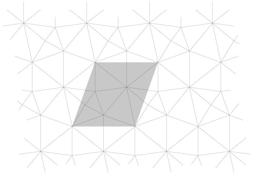
Figure 1. A periodic triangulation, which can be seen as the universal cover of a triangulation of the torus. In gray is one fundamental domain.

A (perhaps) more explicit construction of the Riemann surface $M_{G}$ associated to a triangulation goes as follows. Pick any embedding of $G$ in $\mathbb{T}$ such that edges are mapped to straight line segments. Then, lift the embedding to the whole plane $\mathbb{R}^{2}$, to get a doubly periodic triangulation of it. This doubly periodic graph has a fundamental domain, which is a parallelogram; the shape of this parallelogram can be chosen arbitrarily (it correspond to giving an additional structure to the torus $\mathbb{T}$), but for convenience assume that one of its edges is the unit segment along the first coordinate axis.

Identify $\mathbb{R}^{2}$ to the complex plane $\mathbb{C}$; and for each triangular face $f$ thus obtained, let

(1) $$\mu_{f}:=-\frac{a+\tau b+\tau^{2}c}{\bar{a}+\tau\bar{b}+\tau^{2}\bar{c}}$$

(where $a$, $b$ and $c$ are the vertices of $f$, ordered in the positive direction around the face and seen as complex numbers, and where $\tau=e^{2\pi i/3}$).

Notice that $\mu_{f}$ vanishes if and only if $f$ is an equilateral triangle; and that it is invariant under cyclic relabelling of the vertices, so that it is well-defined. The strict inequality $|\mu_{f}|<1$ is satisfied as soon as none of the faces of the triangulation is degenerate, which we will implicitly assume. In fact, it is easy to check that if $\varphi_{f}$ is any real-linear function mapping $f$ into an equilateral triangle, and preserving orientation, then it has constant Beltrami coefficient

(2) $$\frac{\partial_{\bar{z}}\varphi_{f}}{\partial_{z}\varphi_{f}}=\mu_{f}.$$

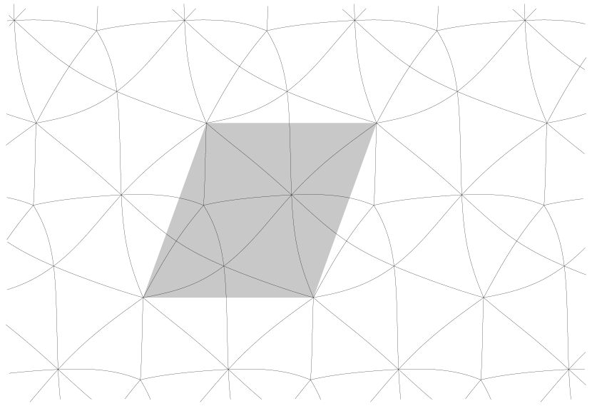
Figure 2. The image of the triangulation of Figure 1 by the corresponding bi-periodic quasi-conformal map $\varphi_{G}$. The gray fundamental domain has vertices $0$, $1$, $\tau_{G}$ and $1+\tau_{G}$.

Now, let $\mu:\mathbb{C}\to\mathbb{C}$ be equal to $\mu_{f}$ in the interior of each face $f$, and to $0$ along edges and at vertices. By periodicity, $\|\mu\|_{\infty}<1$, so by the measurable Riemann mapping theorem (for this and more background on quasi-conformal maps in general, cf. [1]) there exists a quasi-conformal map $\varphi_{G}:\mathbb{C}\to\mathbb{C}$ with Beltrami coefficient $\mu$. This map is unique if one adds the conditions that $\varphi_{G}(0)=0$ and $\varphi_{G}(1)=1$. Moreover, it preserves the periodicity of the initial lattice: there exists a complex number $\tau_{G}\in\mathbb{H}$ such that for any integers $x$ and $y$, and any complex $z$,

(3) $$\varphi_{G}(z+x+iy)=\varphi_{G}(z)+x+\tau_{G}y.$$

What this implies is that $\varphi_{G}$ passes to the quotient, leading to a map

(4) $$\Phi_{G}:\mathbb{R}^{2}/\mathbb{Z}^{2}\to\mathbb{C}/(\mathbb{Z}+\tau_{G}\mathbb{Z})=:\mathbb{T}_{G}.$$

The way that $\mu_{f}$ is chosen, corresponding to the linear map from $f$ to an equilateral triangle, directly implies the following result, which we state as a lemma for easier reference:

Lemma 1.

$\mathbb{T}_{G}$ is conformally equivalent to $M_{G}$.

One can also look at the image of the initial triangulation by the map $\varphi_{G}$ (see Figure 2). This provides a canonical embedding of $G$ in the plane; we will see later that it is for this choice of embedding that the real-linear map in the statement of Theorem 2 it the identity. Notice that if the triangulation is embedded with this fundamental domain to start with, then the difference $\varphi_{G}(z)-z$ is uniformly bounded.

1.3. Subdivisions

Let $T=(V,E)$ be a triangulation of the torus. We construct a subdivision $T^{\prime}$ of $T$, as follows (see Figure 3). The set of vertices of $T^{\prime}$ is $V(T^{\prime})=V\cup E$; two vertices $v_{1}$, $v_{2}\in V(T^{\prime})$ are adjacent if and only if

• one is a vertex of $T$ and the other one is an edge of $T$ incident to that vertex; or,

• both are edges of $T$, incident to a common vertex and a common face.

Figure 3. Subdivision of a triangulation (left: four adjacent faces of $T$; right: the corresponding faces of $T^{\prime}$)

More intuitively, this amounts to replacing each face of $T$ by its subdivision into $4$ triangles, with a new vertex located on each edge of $T$. This construction can then be iterated (see Figure 4); we will denote by $T^{(n)}$ the triangulation obtained from $T$ after $n$ successive subdivisions. The operation of subdivision is a priori combinatorial, but in the case of embedded triangulation, we will always embed the result of the subdivision in such a way that every new vertex is at the midpoint of the corresponding (embedded) edge. This in turn implies that the length of every edge of the subdivided graph is one half of that of some edge of the initial one.

A key remark for what follows is that the structure of $T^{(n)}$ can be described in a simple way starting from that of $T$: it can be obtained by replacing each face of $T$ with a large triangular region of side length $2^{n}$ of the regular triangular lattice. In particular, all the newly added vertices have degree equal to $6$. More importantly, the complex structure introduced in the previous section is not affected by the operation:

Figure 4. Subsequent subdivisions of the triangulation in Figure 3

Lemma 2.

The Riemann surfaces $M_{T}$ and $M_{T^{\prime}}$ are conformally equivalent.

Proof.

This is clear from the construction of $M_{T}$ and $M_{T^{\prime}}$; an explicit conformal map between the two can be constructed from the map $z\mapsto 2z$ in the complex plane. Alternatively, noticing that all the triangles contained in one of the original faces of the triangulation have the same shape, and thus the same value for $\mu_{f}$, the conformal equivalence is a direct consequence of Lemma 1. ∎

Remark 2.

The fact that the subdivisions that we define here are dyadic is mainly for ease of notation; one could as well replace each triangular face of $T$ with a triangular region of side length $N$ for other values of $N$. This will be implied when considering the refined triangulation $\mathcal{T}_{\delta,N}$.

1.4. Other topologies

The same constructions as above can be performed in other settings; most useful for us, but postponed to here because they necessitate a little more notation, is the case of approximations of simply connected domain in the complex plane, or subdivisions of planar triangulations with a boundary.

Let $G$ be a planar graph with one marked face, embedded in the plane in such a way that the marked face is the only unbounded one; we will refer to that face as the outer face of $G$. Assume that all inner faces of $G$ are triangles; to avoid degenerate cases, we will always also assume that the outer face of $G$ has at least $4$ vertices. This last restriction is not an essential one: we are going to investigate finer and finer subdivisions of a fixed graph, and after one such subdivision the outer face cannot have less than $6$ vertices in any case, so up to using the result of the first subdivision as the initial graph, the condition can be assumed to be satisfied.

By welding together equilateral triangles according to the combinatorics of the inner faces of $G$, one can construct a complex structure in the complement of the outer face. Accordingly, to every choice of $4$ boundary vertices $(a,b,c,d)$ of $G$ with appropriate ordering, there corresponds a unique modulus $\rho=\rho_{G}(a,b,c,d)\in\mathbb{R}_{+}$ and a unique conformal map $\Psi_{G;a,b,c,d}$ from the complement of the outer face (equipped with this complex structure) to the rectangle $\mathfrak{R}_{\rho}=[0,\rho_{G}(a,b,c,d)]\times[0,1]\subset\mathbb{R}^{2}\simeq\mathbb{C}$, mapping $a$ (resp. $b$, $c$, $d$) to $\rho$ (resp. $\rho+i$, $i$, $0$).

As before, the modulus $\rho_{G}(a,b,c,d)$ is invariant under the subdivision described earlier:

(5) $$\rho_{G}(a,b,c,d)=\rho_{G^{\prime}}(a,b,c,d).$$

In addition, it is easy to check that under successive refinements, the mesh of the image of $G^{(n)}$ under $\Psi=\Psi_{G^{(n)};a,b,c,d}$, i.e. the largest diameter of the image of a face of $G^{(n)}$, goes to $0$ exponentially fast in $n$. That makes the setup right for the study of scaling limits. Yet as before, seen as a map between domains of the complex plane, the map $\Psi$ is quasi-conformal and its Beltrami derivative is constant on each face of the triangulation, given by the same formula as above.

We now have all the necessary notation to precisely state our first main result. Recall that $\mathfrak{C}(\rho)$ is the limiting crossing probability for critical site-percolation on the triangular lattice, as given by Cardy’s formula.

Theorem 3.

With the previous setup, consider site-percolation at parameter $1/2$ on the vertices of $G^{(n)}$, and let $C_{n}$ be the event that there exists a path of open vertices crossing it between the boundary arcs $(ab)$ and $(cd)$. Then as $n\to\infty$,

$$P[C_{n}]\to\mathfrak{C}(\rho_{G}(a,b,c,d)).$$

2. Macroscopic triangulations

2.1. Framework of the proof

We first focus on the macroscopic case, i.e. for now we consider percolation on successive refinements of a fixed triangulation of a planar domain (in other words, $\delta$ is fixed in this section). Theorem 3 above is stated in this setup.

One possible idea to prove Theorem 3 would be to first focus at the contents of an individual face, and state that in the scaling limit one gets a continuous object described using for instance $CLE_{6}$. The restriction of $G^{(n)}$ to a face of $G$ is indeed an affine deformation of the usual triangular lattice, so the scaling limit of percolation on it, while deformed accordingly, would still be essentially the same as that of percolation on the regular case.

The main difficulty would then be to somehow connect these scaling limits across edges of $G$, in a precise enough way to obtain an exact limit. Unfortunately, this seems to be extremely difficult if not impossible to do with this level of precision. Writing $G$ as a union of overlapping lozenges (intersecting on faces) goes some way in this direction but seems to be insufficient to get explicit limits. Proving convergence directly at the level of the exploration process first and deriving crossing probabilities from it is actually doable, but the direct approach that we apply instead is more robust in the sense that it will readily extend to the mesoscopic case.

2.2. Setup and notation

We actually follow Smirnov’s original proof quite closely, and refer the reader to the articles [10] and [2] for a more detailed version of some of the steps below; rather than reproducing every argument, we point to the relevant differences as we go. The argument has two main steps:

• first, show a compactness result in order to be able to extract subsequential limits of suitable quantities;

• then identify the unique possible subsequential limit, by showing a conformal invariance property.

The choice of the quantity of interest, and the first step of the proof, are extremely similar to their counterparts in Smirnov’s article [11]. Only the identification is really different.

Let $\Omega$ be the simply connected domain in the plane triangulated by $G^{(n)}$. If $f$ is a face of $G^{(n)}$ (or equivalently, a vertex of its dual graph), let $E_{a}^{(n)}(f)$ be the event that there exists a chain of pairwise distinct black vertices of $G^{(n)}$ joining two boundary points of $\Omega$ and separating it into two regions, one containing $a$ and $f$ and the other one containing $b$ and $c$. Let $H_{a}^{(n)}$ be the probability of that event; define $H_{b}^{(n)}$ and $H_{c}^{(n)}$ similarly, in the obvious fashion. Recall that $\tau=e^{2\pi i/3}$, and define

$$H^{(n)}:=H_{a}^{(n)}+\tau H_{b}^{(n)}+\tau^{2}H_{c}^{(n)}$$

(considered as a function from $\Omega$ to $\mathbb{C}$ that is constant on the faces of $G^{(n)}$). The main result will be a consequence of the following:

Proposition 1.

As $n\to\infty$, $H^{(n)}$ converges uniformly to the unique quasi-conformal map $h:\Omega\to\mathbb{C}$ which maps $\Omega$ to the equilateral triangle with vertices $(1,\tau,\tau^{2})$, $a$ (resp. $b$, $c$) to $1$ (resp. $\tau$, $\tau^{2}$), and with Beltrami coefficient $\mu$ chosen according to (1).

Indeed, once this proposition is known to hold, it is enough to look at the observable $H^{(n)}$, and at its limit $h$, at a boundary point $d$ to obtain the value of the corresponding crossing probability.

2.3. Compactness and RSW estimates

The first argument is one of uniform continuity. We first state a result similar to the classical Russo-Seymour-Welsh estimate:

Proposition 2.

For every $\lambda>1$ there exists $c>0$ such that the following holds. Let $\mathfrak{R}$ be a rectangle of aspect ratio $\lambda$, entirely contained in $\Omega$. Then, for every $n$ large enough, the probability that percolation at parameter $1/2$ on $G^{(n)}$ contains a path of black vertices crossing $\mathfrak{R}$ lengthwise is contained in $[c,1-c]$.

Proof.

The result is well-known in the case of the regular triangular lattice. In particular, there is nothing to prove if the rectangle $\mathfrak{R}$ is entirely contained within one of the faces of the initial triangulation $G$. We give a brief explanation of how to extend it to the general case.

Let $\mathfrak{R}$ be a fixed rectangle. There exists a thinner rectangle $\mathfrak{R}^{\prime}$ contained in $\mathfrak{R}$, such that any crossing of $\mathfrak{R}^{\prime}$ also crosses $\mathfrak{R}$, and which contains no vertex of $G$ and intersects a certain number of edges of $G$ transversally. Now, between each pair of successive such edges, $\mathfrak{R}^{\prime}$ intersects $G^{(n)}$ as a piece of the usual triangular lattice, so each of these “sections” is crossed in both directions with positive probability. On the other hand, the union of two successive sections is still isomorphic, as a graph, to a piece of the triangular lattice, so every such union is crossed lengthwise with positive probability. By the Harris-FKG inequality, all of these crossings exist simultaneously with positive probability, and when they do, their union contains a crossing of $\mathfrak{R}^{\prime}$ and hence of $\mathfrak{R}$.

It is easy to obtain uniformity in the estimate, for a given aspect ratio of $\mathfrak{R}$, because the graph $G$ is finite — this is where the mesoscopic case will be more involved. For instance, by a pigeonhole argument, $\mathfrak{R}^{\prime}$ can be chosen with a width at least equal to $|V(G)|^{-1}$ times that of $\mathfrak{R}$. ∎

Proposition 3.

There exist two constants $\varepsilon>0$, $K<\infty$ such that the following holds. Let $n>0$; let $f_{1}$ and $f_{2}$ be two faces of $G^{(n)}$, and denote by $d(f_{1},f_{2})$ the distance between them, either in the Hausdorff sense, or equivalently the Euclidean distance between their centers. Then,

$$|H^{(n)}(f_{2})-H^{(n)}(f_{1})|\leqslant Kd(f_{1},f_{2})^{\varepsilon}.$$

In particular, the family $(H^{(n)})$ is relatively compact for the topology of uniform convergence: any sequence $n_{k}\to\infty$ has a subsequence $(n_{j(k)})$ along which $H^{(n_{j(k)})}$ converges uniformly to an $\varepsilon$-Hölder function defined on $\Omega$.

Proof.

The core of the argument is the same as in Smirnov’s article: if a self-avoiding circuit of black vertices surround both $f_{1}$ and $f_{2}$ then either the events $E_{a}^{(n)}(f_{1})$ and $E_{a}^{(n)}(f_{2})$ are both realized, or none of them is. Consequently, the difference in the statement of the lemma is bounded above by the probability that no such circuit exists. But this last probability is at most of polynomial order in the distance between the two faces, which can be proved using RSW estimates. ∎

2.4. Identification of the limit

The central result of this section is the following:

Proposition 4.

Let $h$ be any subsequential limit of the sequence $(h_{n})$: then $h$ is quasi-conformal on $\Omega$, and on each face $f$ of $G$ its Beltrami coefficient is a.e. equal to $\mu_{f}$.

Proof.

The argument is actually rather simple. Let $f$ be a face of $G$. There exists a continuous, one-to-one map $\sigma_{f}:\Omega\to\mathbb{C}$ which is real-linear within each face of $G$ and maps $f$ itself to an equilateral triangle. This map is quasi-conformal and its Beltrami coefficient in $f$ is equal to $\mu_{f}$. We will use $\sigma_{f}$ to look at percolation “from the point of view of the face $f$”.

For $n>0$, let $h_{n}^{\sigma}=h_{n}\circ\sigma_{f}^{-1}$ be defined on $\sigma_{f}(\Omega)$. Because the definition of $h_{n}$ is purely combinatorial in nature, $h_{n}^{\sigma}$ is exactly the observable that one would get if $G$ were embedded as its image by $\sigma_{f}$. In particular, it shares all its local features, most notably the color-switching lemma. Moreover, convergence is conserved by right composition with $\sigma_{f}^{-1}$: fix a subsequential limit $h$ of $(h_{n})$ and let $h^{\sigma}=h\circ\sigma^{-1}$, defined on $\sigma_{f}(\Omega_{G})$ as well.

The key remark is now that the initial proof of Smirnov is fundamentally local: copying it mutatis mutandis, one gets that the contour integral of $h^{\sigma}$ along each closed contour contained in $\sigma_{f}(f)$ vanishes. This means that $h^{\sigma}$ is holomorphic in $\sigma_{f}(f)$, and in turn that $h$ is quasi-conformal on $f$ and has the same Beltrami derivative on it as $\sigma_{f}$. ∎

Now, let $h$ be a subsequential limit of $(h_{n})$. Remember the definition of the map $\Psi$ in the previous section; it solves the same Beltrami equation as $h$, which means that they are related to one another by left-composition by a conformal map. In other words, the map $g:=h\circ\Psi^{-1}$ is a holomorphic map on the rectangle $[0,\rho]\times[0,1]$. The rest of the discussion is then exactly the same as in the regular case: $g$ has its image contained in the triangle with vertices $(1,\tau,\tau^{2})$, maps boundary to boundary homeomorphically, and from known boundary values, one can then conclude that $g$ is the unique conformal map from the rectangle to the equilateral triangle with these properties, which concludes the proof.

3. Mesoscopic triangulations

We now turn to the proof of convergence in the case of mesoscopic triangulations, i.e. as both $\delta\to 0$ and $N\to\infty$ simultaneously. The overall framework of the argument is the same as before, but more care is needed in order to control the convergence to $0$ of contour integrals, and in addition the Russo-Seymour-Welsh estimate is not a direct consequence of the classical one.

Intuitively, the slower $N$ increases relative to $\delta$, the harder the proof becomes — and indeed the bounded $N$ situation would be full universality for percolation on triangulations, which is very much beyond reach. In fact, it is far from clear whether embedding using welded equilateral triangles remains relevant in that case, although it is certainly the right thing to do as soon as $N$ does tend to infinity.

3.1. Main assumption: uniform RSW estimates

We begin as before with a priori estimates for crossing probability. Consider the lattice $\mathcal{T}_{\delta,N}$ on which site-percolation for parameter $1/2$ is defined. Moreover, choose a rectangle $\mathfrak{R}$ of aspect ratio $\lambda>1$. We will from now on assume that the following holds.

Assumption 1.

There exists a constant $c=c(\lambda)$ depending on $\lambda$ but not on the size or the orientation of $\mathfrak{R}$ such that, uniformly as $\delta\to 0$ and $N\to\infty$, the probability that $\mathfrak{R}$ is crossed in the long direction is contained in $[c,1-c]$.

It is equivalent to make the assumption for one particular value of $\lambda>1$ and to make it for all $\lambda>1$, because crossings of longer rectangles can easily be constructed from unions of crossings of shorter ones. In the previous section, a priori estimates on crossing probabilities were used to obtain the uniform equicontinuity of the observable as the lattice gets finer and finer: this will still be the case here; we refer the reader to the last section of this paper for more remarks about this assumption.

3.2. The setup of the proof

Let $\Omega$ be a simply connected domain of the plane with $3$ points $a$, $b$ and $c$ on its boundary, in positive order; fix $\delta>0$ and $N>0$ for now (with the understanding that $\delta$ will go to $0$ and simultaneously $N$ will go to infinity). Let $\mathcal{T}_{\delta,N}$ be the triangulation of the plane described in the first introduction; we will call cells the faces of the rescaled but not yet subdivided triangulation. The length of an edge of $\mathcal{T}_{\delta,N}$ is of order $\delta/N$, and the diameter of one of its cells is of order $\delta$. Let $\Phi_{\delta}:\mathbb{C}\to\mathbb{C}$ be the quasi-conformal map constructed in the previous section, with Beltrami coefficient given by (1) — since all the faces within a cell have the same shape, $\Phi_{\delta}$ indeed depends on $\delta$ but not on $N$.

We will re-use some of the notation in [2]. If $z$ is a (triangular) face of $\mathcal{T}_{\delta,N}$, or equivalently a vertex of its dual graph, let $H^{(\delta,N)}_{a}(z)$ be the probability that, for critical site-percolation on $\Omega\cap\mathcal{T}_{\delta,N}$, there is a chain of pairwise distinct black vertices joining two boundary vertices and separating $a$ and $z$ on one side and $b$ and $c$ on the other. As before, define $H^{(\delta,N)}_{b}$ and $H^{(\delta,N)}_{c}$ accordingly, and let

(6) $$H^{(\delta,N)}=H^{(\delta,N)}_{a}+\tau H^{(\delta,N)}_{b}+\tau^{2}H^{(\delta,N)}_{c}.$$

As long as no confusion can arise, we will drop $\delta$ and $N$ from the notation and simply refer to $H$ and $\Phi$ where appropriate.

We want to show that a suitable continuous interpolation of $H^{(\delta,N)}$ is approximately quasi-conformal on $\Omega$ with the same Beltrami coefficient as $\Phi_{\delta}$. To do that, we will use the characterization in Appendix A; so, let $\gamma$ be a closed, smooth curve contained in $\Omega$, and let $\gamma_{\delta,N}=(z_{k})_{k=0..L-1}$ be a nearest-neighbor chain of pairwise distinct vertices of $\mathcal{T}_{\delta,N}^{*}$ which approximates $\gamma$ (for ease of notation, let $z_{L}=z_{0}$). Finally, let

(7) $$I:=\sum_{k=0}^{L-1}\frac{H(z_{k+1})+H(z_{k})}{2}[\Phi(z_{k+1})-\Phi(z_{k})].$$

This is the discrete counterpart of the contour integral in the quasi-conformal version of Morera’s lemma, so what we need to show is that $|I|$ is small for appropriate choices of $\delta$ and $N$.

The beginning of the argument goes the same way as for the triangular lattice. If $F$ is a function on $\Omega\cap\mathcal{T}^{\ast}_{\delta,N}$, and if $e=(\underline{e},\overline{e})$, is an oriented edge of $\mathcal{T}^{\ast}_{\delta,N}$, let

(8) $$F(e):=\frac{F(\underline{e})+F(\overline{e})}{2};\qquad\partial_{e}F:=F(\overline{e})-F(\underline{e}).$$

Then $I$ can be rewritten as $I=\sum_{e\in\gamma_{\delta,N}}H(e)\partial_{e}\Phi$. Let $\mathcal{F}$ be the set of all the dual faces surrounded by $\gamma_{\delta,N}$; if $f\in\mathcal{F}$, let $\partial f$ be its boundary, read counterclockwise as a set of oriented edges. Then, since inner edges are counted once in each orientation, one can rewrite

(9) $$I=\sum_{f\in\mathcal{F}}\sum_{e\in\partial f}H(e)\partial_{e}\Phi.$$

For every face $f$ of $\mathcal{T}^{\ast}_{\delta,N}$, let $c_{f}$ be the vertex of $\mathcal{T}_{\delta,N}$ contained in $f$. It is easy to verify, reindexing the sums involved above (see [2] for the details), that one has the identity

(10) $$I=-\sum_{f\in\mathcal{F}}\sum_{e\in\partial f}\partial_{e}H[\Phi(e)-\Phi(c_{f})].$$

There are two kinds of edges in that sum. For those on the path $\gamma_{\delta,N}$, we know from Russo-Seymour-Welsh estimates (which hold due to Assertion 1) that $\partial_{e}H=\mathcal{O}((\delta/N)^{\eta})$ for some positive $\eta$; together with the fact that $\Phi(e)-\Phi(c_{f})=\mathcal{O}(\delta/N)$ and choosing $\gamma_{\delta,N}$ with $L=\mathcal{O}(N/\delta)$, which is always possible, the sum over all such edges ends up providing a term of order $(\delta/N)^{\eta}$. For edges inside the curve, each term of the form $\partial_{e}H\Phi(e)$ appears twice with different sign, so they cancel out. Denoting by $e^{*}$ the dual edge of $e$ (which makes it an edge of $\mathcal{T}_{\delta,N}$), oriented so that the rotation from $e$ to $e^{*}$ goes in the positive direction, this gives

(11) $$I=\sum_{e}\partial_{e}H\partial_{e^{*}}\Phi+\mathcal{O}((\delta/N)^{\eta}),$$

where the sum ranges over all the edges of $\mathcal{T}_{\delta,N}^{*}$ surrounded by $\gamma$.

Let $P^{(\delta,N)}_{a}(e)$ be the probability that $\overline{e}$ satisfies the conditions defining $H^{(\delta,N)}_{a}$ but $\underline{e}$ does not; then, $\partial_{e}H_{a}=P_{a}(e)-P_{a}(-e)$, where $-e$ designates the reversal of the edge $e$, and where again for clarity we drop $(\delta,N)$ from the notation. Replacing $H$ by its definition, and reordering the terms to make each edge appear only once, leads to

(12) $$I=2\sum_{e}[P_{a}(e)+\tau P_{b}(e)+\tau^{2}P_{c}(e)]\partial_{e^{*}}\Phi.$$

So far, nothing is very different from the regular triangular lattice case, because we are just doing algebra. The next step is again the same, it uses Smirnov’s “color-switching lemma”, which can be stated as follows. For a given edge $e$ of $\mathcal{T}^{*}_{\delta,N}$, its source $\underline{e}$ has degree $3$; denote by $e^{\prime}$ and $e^{\prime\prime}$ the other two edges sharing the same source, ordered so that $e$, $e^{\prime}$ and $e^{\prime\prime}$ come in that order turning counterclockwise around $\underline{e}$. Then, the lemma is the following identity: for every edge $e$,

(13) $$P_{a}(e)=P_{b}(e^{\prime})=P_{c}(e^{\prime\prime}).$$

The proof is exactly the same again as in the regular case, so we do not repeat it here. Replacing in the previous estimate:

(14) $$I=2\sum_{e}P_{a}(e)[\partial_{e^{*}}\Phi+\tau\partial_{(e^{\prime})^{*}}\Phi+\tau^{2}\partial_{(e^{\prime\prime})^{*}}\Phi]+\mathcal{O}((\delta/N)^{\eta}).$$

In the equilateral case, $\Phi$ is the identity function, the bracket term is identically $0$, and the argument ends here. In the more general case, more work needs to be done. The main image to keep in mind (although it does not explicitly correspond to the proof that follows) is that the image of $\mathcal{T}_{\delta,N}$ by the quasi-conformal map constructed in section 1.2 has almost all its faces almost equilateral — see Figure 5.

Figure 5. The image of $\mathcal{T}_{\delta,N}$ by the corresponding doubly periodic quasi-conformal map; here $\delta=1$ and $N=16$. Away from the initial vertices, the triangles are close to being equilateral.

3.3. Controlling the bracket term

Assume for a moment that the combinatorics of the initial lattice is that of the triangular lattice, but that the embedding is chosen differently. More specifically, one can assume that $\mathcal{T}$ is the square lattice with added diagonals in the north-east direction. Then $\Phi$ is the real-affine map sending it to the regular triangular lattice, in other words it maps every face of $\mathcal{T}_{\delta,N}$ to an equilateral triangle. In that case, the bracket is still identically equal to $0$, so $I$ is uniformly small.

What we will show is that the general case is a small perturbation of that situation, as soon as $N$ is large enough as a function of $\delta$. Let $f$ be a (triangular) face of $\mathcal{T}_{\delta,N}$, and let $c$ be the $\delta$-cell containing it. We first consider the case when $c$ (and therefore $f$ as well) is equilateral. Then the Beltrami coefficient of $\Phi$ vanishes in $c$, in other words $\Phi$ is holomorphic in $c$.

Let $d$ be the distance between $f$ and $\partial c$: then the distorsion theorem states that the second derivative of $\Phi$ inside $f$ is dominated by $\mathcal{O}(|\Phi^{\prime}|/d)$, in addition to which $\Phi^{\prime}$ is uniformly bounded on $c$. We can then do a Taylor expansion of the bracket term in (14) corresponding to $f$. The constant term vanishes, and so does the first-derivative one because the tangent map is a complex multiplication which still sends $f$ to an equilateral triangle. The bracket then reduces to

(15) $$\mathcal{O}((\delta/N)^{2}|\Phi^{\prime\prime}|)=\mathcal{O}((\delta/N)^{2}/d).$$

It remains to control the sum over $c$ of that estimate. The number of faces at distance $k\delta/N$ of the cell boundary is of order $N$, so the sum over $c$ of the bracket terms is bounded, up to a multiplicative constant, by

(16) $$\sum_{k=1}^{N}N(\delta/N)^{2}(N/k\delta)\simeq\delta\log N.$$

This bound is not at all optimal, because near the common boundary of two adjacent equilateral cells, $\Phi$ will still be analytic: $d$ could be replaced by the distance to the boundary of the lozenge formed by these two cells. What we will keep from that remark is that the faces of $\mathcal{T}_{\delta,N}$ along the boundary of $c$ (where $d=0$) do not contribute enough to the previous estimate to change its order of magnitude. As for the $3$ triangles near the vertices of $c$, the fact that $\Phi$ is Hölder shows that they have a bracket of order at most a positive power of $\delta/N$, and still do not contribute to the estimate above.

Actually, not much needs to be changed in the argument if the cell $c$ is not equilateral: one can, as in the macroscopic case in the previous section, pre-compose everything by a real-affine map $\Psi$ of the whole plane sending $c$ to an equilateral triangle of the same diameter. Then $\Phi\circ\Psi^{-1}$ is analytic on $\Psi(c)$, and the reasoning of the previous paragraph applies to it mutatis mutandis.

It still remains to take the sum over all the cells surrounded by $\gamma$. There are of order $\delta^{-2}$ of these. Besides, the term $P_{a}(e)$ is, from RSW estimates, bounded above by $(\delta/N)^{\eta^{\prime}}$ for some $\eta^{\prime}>0$. Putting everything together, we obtain

$$I=\mathcal{O}((\delta/N)^{\eta})+\mathcal{O}(\delta^{\eta^{\prime}-2}N^{-\eta^{\prime}}\delta\log N)=\mathcal{O}((\delta/N)^{\eta})+\mathcal{O}(\delta^{\eta^{\prime}-1}N^{-\eta^{\prime}}\log N).$$

This means that as soon as $N$ grows fast enough as a function of $\delta$ to make the second error term go to $0$, $I$ will be uniformly controlled. The bound we get is not optimal at all, but for further reference, taking

(17) $$N=\delta^{1-\varepsilon-1/\eta^{\prime}}$$

for arbitrary $\varepsilon>0$ is enough.

Remark 3.

The value of the $3$-arm exponent is expected to be equal to $2/3$, which means that the above convergence of $I$ to $0$ should hold as soon as $N\gg\delta^{-1/2}$ — though of course we have no way to obtain the value of the exponent before proving conformal invariance in the first place.

3.4. Concluding the proof

Now that we have the main estimate on the discrete integral $I$, the remainder of the proof is actually very close to the regular case. Pick a sequence $\delta_{k}\downarrow 0$, choose $N_{k}\to\infty$ satisfying the previous lower bound. Up to a subsequence extraction, we can assume that $(H^{(\delta_{k},N_{k})})$ converges, uniformly on compact subsets of $\Omega$, to some continuous function $h:\Omega\to\mathbb{C}$. Simultaneously, $\Phi_{\delta_{k}}$ converges uniformly to a real-affine map $\Phi_{0}:\mathbb{C}\to\mathbb{C}$. From the previous section, we directly obtain, for any smooth closed curve $\gamma$ contained in $\Omega$,

(18) $$\oint_{\gamma}h(z)\mathrm{d}\Phi_{0}(z)=0.$$

This means that $h\circ\Phi_{0}^{-1}$ is holomorphic, from which the statement follows; $\Phi_{0}$ is the real-linear map appearing in the conclusion of the theorem.

4. Concluding remarks

A key step of the argument above relies on a priori bounds for box-crossings. While this looks like a rather strong assumption, actually a closer look at the proof shows that one can almost get away without it. Indeed, even though we might not have assumption 1, we still have the corresponding statement for boxes contained within a single $\delta$-cell because there the graph structure is that of the triangular lattice (for which box-crossing estimates are known). In particular, the discrete derivative estimates that we used, namely

(19) $$\partial_{e}H=\mathcal{O}((\delta/N)^{\eta})\quad\text{and}\quad P_{a}(e)=\mathcal{O}((\delta/N)^{\eta^{\prime}})$$

can instead be replaced by their counterparts within a $\delta$-cell. This leads to much weaker bounds:

(20) $$\partial_{e}H=\mathcal{O}(N^{-\eta})\quad\text{and}\quad P_{a}(e)=\mathcal{O}(N^{-\eta^{\prime}})$$

but otherwise the proof proceeds without a change. The lower bound for the growth of $N$ in terms of $\delta$ grows like $\delta^{-1/\eta^{\prime}}$ rather than $\delta^{1-1/\eta^{\prime}}$, which is only a little worse.

The only place where I could not get rid of Assumption 1 is in the proof of uniform continuity for the observable. Indeed, for that to hold one needs to control differences in $H$ across different cells, and then the estimate from the triangular lattice alone becomes trivial. On the other hand, all that is needed here is the ability to extract converging subsequences as the lattice mesh vanishes; uniform Hölder estimates are a nice way to get that, but perhaps a weaker version of equicontinuity can be obtained (for instance from the information, which we do have, that there is no infinite cluster at the critical point).

One last, more positive remark about assumption 1 is in order: while none of the known proofs of box-crossing estimates seems to apply uniformly in $(\delta,N)$ in the general case, as soon as the initial lattice has more symmetry (for instance, if in addition to its periodicity it has an embedding that is invariant under a $90$-degree rotation) they can be extended and do provide the necessary bounds. In that case, symmetry implies also that the modulus $\tau_{G}$ constructed in the first section is actually equal to $i$, and the whole picture is much more explicit.

Appendix A An integral characterization of qc maps

Let $\Omega$ be a simply connected domain, and $\mu:\Omega\to\mathbb{C}$ be piecewise continuous and such that $\|\mu\|_{\infty}<1$. Fix $\varphi_{0}:\Omega\to\mathbb{C}$ solution to the Beltrami equation with coefficient $\mu$.

Proposition 5.

With the above notation, a continuous, injective function $\varphi:\Omega\to\mathbb{C}$ is itself solution to the Beltrami equation with coefficient $\mu$ if and only if for any Jordan curve $\gamma$ in $\Omega$, one has

$$\oint_{\gamma}\varphi(z)d\varphi_{0}(z)=\oint_{\gamma}\varphi(z)\;\partial_{z}\varphi_{0}(z)\;[dz+\mu(z)d\bar{z}]=0.$$

Proof.

Let $g=\varphi\circ\varphi_{0}^{-1}$. $\varphi$ is quasi-conformal with Beltrami coefficient $\mu$ if and only if $g$ is holomorphic, and this in turn can be characterized using Morera’s theorem: it is the case if and only if for every closed curve $\gamma_{0}$ in $\varphi_{0}(\Omega)$,

$$\oint_{\gamma_{0}}[\varphi\circ\varphi_{0}^{-1}](w)dw=0.$$

It is just a matter of changing variables, letting $w=\varphi_{0}(z)$ and $\gamma=\varphi_{0}^{-1}\circ\gamma_{0}$, to get

$$\oint_{\gamma_{0}}[\varphi\circ\varphi_{0}^{-1}](w)dw=\oint_{\gamma}\varphi(z)d\varphi_{0}(z).$$

In more geometric terms, all the proof amounts to saying is that the data of $\mu$ endows $\Omega$ with a complex structure and therefore a notion of holomorphic function, and that in a given chart ($\varphi_{0}$ here), those are usual analytic function characterized for instance by an integral formula. ∎

Appendix B About the pictures, and circle packings

Solving the Beltrami equation of section 1.2 analytically is usually impossible to do, and even though it is known that $\tau_{G}$ is always an algebraic number, computing its minimal polynomial seems to be beyond the reach of systematic methods. Solving the Beltrami equation numerically is quite involved. On the other hand, an approximation that is good enough for the purpose of e.g. generating Figure 2 can be obtained using circle packings.

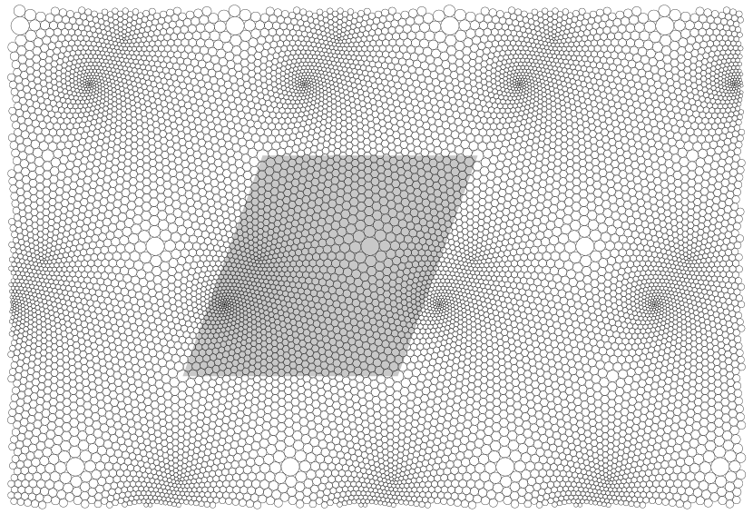
Figure 6. The circle packing obtained from $\mathcal{T}_{1,N}$, where $\mathcal{T}$ is the triangulation in Figure 1 and $N=16$.

More specifically, keeping $\delta=1$, to the triangulation $\mathcal{T}_{1,N}$ described in the introduction corresponds an essentially unique circle packing in the plane (see Figure 6), which is a collection of disks of disjoint interiors, indexed by the vertices of $\mathcal{T}_{1,N}$, and such that two disks are tangent if and only if the corresponding vertices are adjacent (two such packings are conjugated by a global map of the form $az+b$, and one can normalize the choice by imposing that $0$ and $1$ are the centers of the disks corresponding to the vertices that are at these locations in Figure 1).

One can then re-embed $\mathcal{T}_{1,N}$ in the plane by mapping each vertex to the center of the corresponding disk; this map can be extended to a piecewise linear map $\psi_{N}:\mathbb{C}\to\mathbb{C}$ by interpolation on the faces of $\mathcal{T}_{1,N}$. In fact, it is possible to show that as $N\to\infty$, $\psi_{N}$ converges uniformly to the map $\phi_{G}$ constructed in section 1.2. Figure 2 was obtained by drawing the images by $\psi_{N}$ of the edges of $\mathcal{T}_{1,\delta}$ lying along edges of the initial triangulation $\mathcal{T}$ (here $N=16$), and Figure 5 by simply keeping all the edges.

References

- [1] L. V. Ahlfors, Lectures on quasiconformal mappings, vol. 38 of University Lecture Series, American Mathematical Society, Providence, RI, second ed., 2006. With supplemental chapters by C. J. Earle, I. Kra, M. Shishikura and J. H. Hubbard.
- [2] V. Beffara, Cardy’s formula on the triangular lattice, the easy way, in Universality and Renormalization, I. Binder and D. Kreimer, eds., vol. 50 of Fields Institute Communications, The Fields Institute, 2007, pp. 39–45.
- [3] J. Cardy, Critical percolation in finite geometries, 25 (1992), pp. L201–L206.
- [4] G. R. Grimmett, Percolation, vol. 321, Springer-Verlag, Berlin, second ed., 1999.
- [5] H. Kesten, The critical probability of bond percolation on the square lattice equals , 74 (1980), pp. 41–59.
- [6] , Percolation theory for mathematicians, vol. 2 of Progress in Probability and Statistics, Birkhäuser, Boston, Mass., 1982.
- [7] S. K. Lando and A. K. Zvonkin, Graphs on surfaces and their applications, vol. 141 of Encyclopaedia of Mathematical Sciences, Springer-Verlag, Berlin, 2004. With an appendix by Don B. Zagier, Low-Dimensional Topology, II.
- [8] L. Russo, A note on percolation, 43 (1978), pp. 39–48.
- [9] P. D. Seymour and D. J. A. Welsh, Percolation probabilities on the square lattice, 3 (1978), pp. 227–245. Advances in graph theory (Cambridge Combinatorial Conf., Trinity College, Cambridge, 1977).
- [10] S. Smirnov, Critical percolation in the plane: Conformal invariance, Cardy’s formula, scaling limits, 333 (2001), pp. 239–244.
- [11] , Critical percolation in the plane. I. Conformal invariance and Cardy’s formula. II. Continuum scaling limit. http://www.math.kth.se/~stas/papers/percol.ps, 2001.
- [12] S. Smirnov and W. Werner, Critical exponents for two-dimensional percolation, Mathematical Research Letters, 8 (2001), pp. 729–744.