Some remarks on spatial uniformity of solutions of reaction-diffusion PDE’s and a related synchronization problem for ODE’s

Abstract

In this note, we present a condition which guarantees spatial uniformity for the asymptotic behavior of the solutions of a reaction-diffusion PDE with Neumann boundary conditions in one dimension, using the Jacobian matrix of the reaction term and the first Dirichlet eigenvalue of the Laplacian operator on the given spatial domain. We also derive an analog of this PDE result for the synchronization of a network of identical ODE models coupled by diffusion terms.

1 Introduction

Global stability is a central research topic in dynamical systems theory. Stability properties are typically defined in terms of attraction to an invariant set, for example to an equilibrium or a periodic orbit, often coupled with a Lyapunov stability requirement that trajectories that start near the attractor must stay close to the attractor for all future times.

A far stronger requirement than attraction to a pre-specified target set is to ask that any two trajectories should (exponentially, and with no overshoot) converge to each other, or, in more abstract mathematical terms, that the flow be a contraction in the state space. While this requirement will be less likely to be satisfied for a given system, it is sometimes comparatively easier to check. Indeed, checking stability properties often involves constructing an appropriate Lyapunov function, which, in turn, requires a priori knowledge of the attractor location. In contrast, contraction-based methods, discussed here, do not require the prior knowledge of attractors. Instead, one checks an infinitesimal property, that is to say, a property of the vector field defining the system, which guarantees exponential contractivity of the induced flow.

It is useful to first discuss the relatively trivial case of linear time-invariant systems of differential equations $\dot{x}=Ax$, with Euclidean norm. Since differences of solutions are also solutions, contractivity amounts simply to the requirement that there exist a positive number $c$ such that, for all solutions, $\left|x(t)\right|\leq e^{-ct}\left|x(0)\right|$, where $|\cdot|$ refers to the Euclidean norm. This is clearly equivalent to the requirement that $A+A^{T}$ be a negative definite matrix. In Lyapunov-function terms, $x^{T}Px$ is a Lyapunov function for the system, when $P=I$.

This property is of course stronger than merely asymptotic stability of the zero equilibrium of $\dot{x}=Ax$, that is, that $A$ be a Hurwitz matrix (all eigenvalues with negative real part). Of course, asymptotic stability is equivalent to the existence of some positive definite matrix $P$ (but not necessarily the identity) so that $x^{T}Px$ is a Lyapunov function, and this can be interpreted, as remarked later, as a contractivity property with respect to a weighted Euclidean norm associated to $P$. This simple example with linear systems already illustrates why an appropriate choice of norms when defining “contractivity” is critical; even for linear systems, contractivity is not a topological, but is instead a metric property: it depends on the norm being used, in close analogy to the choice of an appropriate Lyapunov function.

The proper tool for characterizing contractivity for nonlinear systems is provided by the matrix measures, also called logarithmic norms (see e.g. [1, 2]), of the Jacobian of the vector field, evaluated at all possible states. This idea is a classical one, and can be traced back at least to work of D.C. Lewis in the 1940s, see [3, 4]. Dahlquist’s 1958 thesis under Hörmander (see [5] for a journal paper) used matrix measures to show contractivity of differential equations, and more generally of differential inequalities, the latter applied to the analysis of convergence of numerical schemes for solving differential equations. Several authors have independently rediscovered the basic ideas. For example, in the 1960s, Demidovič [6, 7] established basic convergence results with respect to Euclidean norms, as did Yoshizawa [8, 9]. In control theory, the field attracted much attention after the work of Lohmiller and Slotine [10], and especially a string of follow-up papers by Slotine and collaborators, see for example [11, 12, 13, 14]. These papers showed the power of contraction techniques for the study of not merely stability, but also observer problems, nonlinear regulation, and synchronization and consensus problems in complex networks. (See also the work by Nijmejer and coworkers [15].) We refer the reader especially to the careful historical analysis given in [16]. Other very useful historical references are [17] and the survey [18].

In this paper, we establish new results for synchronization of diffusively interconnected and identical components, described by nonlinear differential equations. Specifically, we consider interconnected systems $\dot{x_{i}}=f(x_{i},t)+\sum_{j\in N(i)}D(x_{j}-x_{i})$, where the $i$th subsystem (or “agent”) has state $x_{i}(t)$, and show that the difference between any two states goes to zero exponentially, i.e., $\forall i,j$, $(x_{i}-x_{j})(t)\to 0$ as $t\to\infty$. An interconnection graph provides the adjacency structure, and the indices in $N(i)$ represent the “neighbors” of the $i$th subsystem. The matrix $D$ is a diagonal matrix of diffusion strengths. The analysis of synchrony in networks of identical components is a long-standing problem in different fields of science and engineering as well as in mathematics. In biology, the synchronization phenomenon is exhibited at the physiological level, for example in neuronal interactions, in the generation of circadian rhythms, or in the emergence of organized bursting in pancreatic beta-cells, [19, 20, 21, 22, 23, 24]. It is also exhibited at the population level, for example in the simultaneous flashing of fireflies, [25, 26]. In engineering, one finds applications of synchronization ideas in areas as varied as robotics or autonomous vehicles, [27, 28]. Synchronization results based on contraction-based techniques, most by using measures derived from $L^{2}$ or weighted $L^{2}$ norms, have been developed, see for example [10, 29, 30, 31, 12]. For non $L^{2}$ norms, current results are partial, applying only to certain types of graphs. Finding general statements and proofs is still an open problem.

The convergence to uniform solutions in reaction-diffusion partial differential equations $\partial u/\partial t={F(u,t)}+D\Delta u$ where $u=u({\omega},t)$, is a formal analogue of the synchronization of ODE systems. In the analogy, we think of $u(\omega,\cdot)$ as representing an individual system or agent (the index “$i$” in the synchronization problem) whose state is described at time $t$ by $u=u({\omega},t)$. (So $u=u({\omega},t)$ plays the role of $x_{i}(t)$. We use “$u$” to denote the state, instead of $x$, so as to be consistent with standard PDE notations.) Questions of convergence to uniform solutions in reaction-diffusion PDE’s are also a classical topic of research. The “symmetry breaking” phenomenon of diffusion-induced, or Turing, instability refers to the case where a dynamic equilibrium $\bar{u}$ of the non-diffusing ODE system $du/dt=F(u,t)$ is stable, but, at least for some diagonal positive matrices $D$, the corresponding uniform state $u(\omega)=\bar{u}$ is unstable for the PDE system $\partial u/\partial t=F(u,t)+D\Delta u$. This phenomenon has been studied at least since Turing’s seminal work on pattern formation in morphogenesis [32], where he argued that chemicals might react and diffuse so as result in heterogeneous spatial patterns. Subsequent work by Gierer and Meinhardt [33, 34] produced a molecularly plausible minimal model, using two substances that combine local autocatalysis and long-ranging inhibition. Since that early work, a variety of processes in physics, chemistry, biology, and many other areas have been studied from the point of view of diffusive instabilities, and the mathematics of the process has been extensively studied [35, 36, 37, 38, 39, 40, 41, 42, 43, 44]. Most past work has focused on local stability analysis, through the analysis of the instability of nonuniform spatial modes of the linearized PDE. Nonlinear, global, results are usually proved under strong constraints on diffusion constants as they compare to the growth of the reaction part. Contraction techniques add a useful set of tools to that analysis. As with synchronization, for non-Euclidean norms we only provide results in special cases, the general problem being open.

After presenting some mathematical tools in Section 2, we will revisit, in the current context, the biochemical example described in [45, 46] and the Goodwin example studied in [47, 29] in Section 3. Next, in Section 4, we will state and prove the main result of this work: we present a condition which guarantees spatial uniformity for the asymptotic behavior of the solutions of a reaction-diffusion PDE with Neumann boundary conditions in one dimension. We also present some conditions which guarantees contractivity of the solutions of a reaction-diffusion PDE with Dirichlet boundary conditions. We may think of convergence to spatially uniform solutions as a sort of “synchronization” of independent “agents”, one at each spatial location, and each evolving according to a dynamics specified by an ODE. In that interpretation, our work is related to a large literature on synchronization of discrete groups of agents connected by diffusion, whose interconnections are specified by an undirected graph. In that spirit, in Section 5 we derive an analog of our PDE result to the synchronization of a network of identical ODE models coupled by diffusion terms through different types of graphs, including line, complete, and star graphs, and Cartesian products of such graphs.

2 Preliminaries

We now define and state elementary properties of logarithmic Lipschitz constants. (For applications to ODE’s, we will always take $X=Y$ in the definitions to follow.)

Definition 1.

[18] Let $(X,\|\cdot\|_{X})$ be a normed space and $f\colon Y\to X$ be a function, where $Y\subseteq X$. The least upper bound (lub) Lipschitz constant of $f$ induced by the norm $\|\cdot\|_{X}$, on $Y$, is defined by

$$L_{Y,X}[f]=\displaystyle\sup_{u\neq v\in Y}\frac{\|f(u)-f(v)\|_{X}}{\|u-v\|_{X}}.$$

Note that $L_{Y,X}[f]<\infty$ if and only if $f$ is Lipschitz on $Y$.

Definition 2.

[18] Let $(X,\|\cdot\|_{X})$ be a normed space and $f\colon Y\to X$ be a Lipschitz function. The least upper bound (lub) logarithmic Lipschitz constant of $f$ induced by the norm $\|\cdot\|_{X}$, on $Y\subseteq X$, is defined by

$$M_{Y,X}[f]=\displaystyle\lim_{h\to 0+}\frac{1}{h}\left(L_{Y,X}[I+hf]-1\right),$$

or equivalently, it is equal to

$$\lim_{h\to 0^{+}}\sup_{u\neq v\in Y}\frac{1}{h}\left(\frac{\|u-v+h(f(u)-f(v))\|_{X}}{\|u-v\|_{X}}-1\right).$$

If $X=Y$, we write $M_{X}$ instead of $M_{X,X}$.

Notation 1.

Under the conditions of Definition 2, let $M^{\pm}_{Y,X}$ denote

$$\sup_{u\neq v\in Y}\lim_{h\to 0^{\pm}}\frac{1}{h}\left(\frac{\|u-v+h(f(u)-f(v))\|_{X}}{\|u-v\|_{X}}-1\right).$$

If $X=Y$, we write $M^{\pm}_{X}$ instead of $M^{\pm}_{X,X}$.

Remark 1.

[48, 18] Another way to define $M^{\pm}$ is by the concept of semi inner product which is in fact the generalization of inner product to non Hilbert spaces. Let $(X,\|\cdot\|_{X})$ be a normed space. For $x_{1},x_{2}\in X$, the right and left semi inner products are defined by

$$(x_{1},x_{2})_{\pm}=\displaystyle\|x_{1}\|_{X}\lim_{h\to 0^{\pm}}\frac{1}{h}\left(\|x_{1}+hx_{2}\|_{X}-\|x_{1}\|_{X}\right).$$

In particular, when $\|\cdot\|_{X}$ is induced by a true inner product $(\cdot,\cdot)$, (for example when $X$ is a Hilbert space), then $(\cdot,\cdot)_{-}=(\cdot,\cdot)_{+}=(\cdot,\cdot)$.

Using this definition,

$$M_{Y,X}^{\pm}[f]=\displaystyle\sup_{u\neq v\in Y}\frac{(u-v,f(u)-f(v))_{\pm}}{\|u-v\|_{X}^{2}}.$$

The following elementary properties of semi inner products are consequences of the properties of norms. See [48, 18] for a proof.

Proposition 1.

For $x,y,z\in X$ and $\alpha\geq 0$,

1. $(x,-y)_{\pm}=-(x,y)_{\mp}$;

2. $(x,\alpha y)_{\pm}=\alpha(x,y)_{\pm}$;

3. $(x,y)_{-}+(x,z)_{\pm}\leq(x,y+z)_{\pm}\leq(x,y)_{+}+(x,z)_{\pm}$.

Remark 2.

For any operator $f\colon Y\subset X\to X$:

$$M^{-}_{Y,X}[f]\leq M^{+}_{Y,X}[f]\leq M_{Y,X}[f].$$

However, $M^{-}[f]=M^{+}[f]=M[f]$ if the norm is induced by an inner product.

For linear $f$, one has the reverse of the second inequality as well, so $M^{+}_{Y,X}[f]=M_{Y,X}[f]$. See [49] for a detailed proof. When identifying a linear operator $f:{\mathbb{R}}^{n}\rightarrow{\mathbb{R}}^{n}$ with its matrix representation $A$ with respect to the canonical basis, we write “$\mu(A)$” instead of $M^{+}_{X}[f]$, and call $M$ or $\mu$ a “matrix measure”.

Remark 3.

For a linear operator $f$, $M$ and $M^{+}$ can be written as follows:

$$M_{Y,X}[f]=\displaystyle\lim_{h\to 0^{+}}\sup_{u\neq 0\in Y}\frac{1}{h}\left(\frac{\|u+hf(u)\|_{X}}{\|u\|_{X}}-1\right)$$ (1)

and

$$M^{+}_{Y,X}[f]=\displaystyle\sup_{u\neq 0\in Y}\lim_{h\to 0^{+}}\frac{1}{h}\left(\frac{\|u+hf(u)\|_{X}}{\|u\|_{X}}-1\right).$$ (2)

Notation 2.

In this work, for $(X,\|\cdot\|_{X})=({\mathbb{R}}^{n},\|\cdot\|_{p})$, where $\|\cdot\|_{p}$ is the $L^{p}$ norm on ${\mathbb{R}}^{n}$, for some $1\leq p\leq\infty$, we sometimes use the notation “$M_{p}$” instead of $M_{X}$ for the (lub) logarithmic Lipschitz constant, and by “$M_{p,Q}$” we denote the (lub) logarithmic Lipschitz constant induced by the weighted $L^{p}$ norm, $\|u\|_{p,Q}:=\|Qu\|_{p}$ on ${\mathbb{R}}^{n}$, where $Q$ is a fixed nonsingular matrix. Note that $M_{p,Q}[A]=M_{p}[QAQ^{-1}]$.

Remark 4.

In Table 1, the algebraic expression of the least upper bound logarithmic Lipschitz constant induced by the $L^{p}$ norm for $p=1,2,$ and $\infty$ are shown for matrices. For proofs, see for instance [50].

Table 1: Standard matrix measures for a real $n\times n$ matrix, $A=[a_{ij}]$.

vector norm, $\|\cdot\|$	induced matrix measure, $M[A]$
$\|x\|_{1}=\displaystyle\sum_{i=1}^{n}\left|x_{i}\right|$	$M_{1}[A]=\displaystyle\max_{j}\left(a_{jj}+\displaystyle\sum_{i\neq j}\left|a_{ij}\right|\right)$
$\|x\|_{2}=\left(\displaystyle\sum_{i=1}^{n}\left|x_{i}\right|^{2}\right)^{\frac{1}{2}}$	$M_{2}[A]=\displaystyle\max_{\lambda\in\mbox{spec}{\frac{1}{2}(A+A^{T})}}\lambda$
$\|x\|_{\infty}=\displaystyle\max_{1\leq i\leq n}\left|x_{i}\right|$	$M_{\infty}[A]=\displaystyle\max_{i}\left(a_{ii}+\displaystyle\sum_{i\neq j}\left|a_{ij}\right|\right)$

The following subadditivity property is key to diffusive interconnection analysis.

Proposition 2.

[18] Let $(X,\|\cdot\|_{X})$ be a normed space. For any $f$, $g\colon Y\to X$ and any $Y\subseteq X$:

1. $M^{+}_{Y,X}[f+g]\leq M^{+}_{Y,X}[f]+M^{+}_{Y,X}[g]$;

2. $M^{+}_{Y,X}[\alpha f]=\alpha M_{Y,X}[f]$ for $\alpha\geq 0$.

The (lub) logarithmic Lipschitz constant makes sense even if $f$ is not differentiable. However, the constant can be tightly estimated, for differentiable mappings on convex subsets of finite-dimensional spaces, by means of Jacobians.

Lemma 1.

[51] For any given norm on $X={\mathbb{R}}^{n}$, let $M$ be the (lub) logarithmic Lipschitz constant induced by this norm. Let $Y$ be a connected subset of $X={\mathbb{R}}^{n}$. Then for any (globally) Lipschitz and continuously differentiable function $f\colon Y\to{\mathbb{R}}^{n}$,

$$\sup_{x\in Y}M_{X}[J_{f}(x)]\leq M_{Y,X}[f]\,$$

Moreover, if $Y$ is convex, then

$$\sup_{x\in Y}M_{X}[J_{f}(x)]=M_{Y,X}[f]\,.$$

Note that for any $x\in Y$, $J_{f}(x)\colon X\to X$. Therefore, we use $M_{X}$ instead of $M_{X,X}$, as we said in Definition 2.

We also recall a notion of generalized derivative, that can be used when taking derivatives of norms (which are not differentiable).

Definition 3.

The upper left and right Dini derivatives for any continuous function, $\Psi\colon[0,\infty)\to{\mathbb{R}}$, are defined by

$$\begin{array}[]{rcl}\left(D^{\pm}\Psi\right)(t)=\displaystyle\limsup_{h\to 0^{\pm}}\frac{1}{h}\left(\Psi(t+h)-\Psi(t)\right).\end{array}$$

Note that $D^{+}\Psi$ and/or $D^{-}\Psi$ might be infinite.

The following Lemma from [48], indicates the relation between the Dini derivative and the semi inner product.

Lemma 2.

For any bounded linear operator $A\colon X\to X$, and any solution $u\colon[0,T)\to X$ of $\displaystyle\frac{du}{dt}=Au$,

$$D^{+}\|u(t)\|_{X}=\displaystyle\frac{(u(t),Au(t))_{+}}{\|u(t)\|_{X}^{2}}\|u(t)\|_{X}\leq M_{X}[A]\|u(t)\|_{X},$$

for all $t\in[0,T)$.

In this note, we will use the following general result, which estimates rates of contraction (or expansion) among any two functions, even functions that are not solutions of the same system of ODEs (see comment on observers to follow):

Lemma 3.

Let $\left(X,\|\cdot\|_{X}\right)$ be a normed space and $G\colon Y\times[0,\infty)\to X$ be a $C^{1}$ function, where $Y\subseteq X$. Suppose $u,v\colon[0,\infty)\to Y$ satisfy

$$(\dot{u}-\dot{v})(t)\;=\;G_{t}(u(t))-G_{t}(v(t)),$$

where $\dot{u}=\frac{du(t)}{dt}$ and $G_{t}(u)=G(u,t)$. Let

$$c:=\displaystyle\sup_{\tau\in[0,\infty)}M_{Y,X}\;[{G_{\tau}}].$$

Then for all $t\in[0,\infty)$,

$$\|u(t)-v(t)\|_{X}\;\leq\;e^{ct}\|u(0)-v(0)\|_{X}.$$ (3)

Proof.

Using the definition of Dini derivative, we have (dropping the argument $t$ for simplicity):

$$\!\!\!\!\!\!\!\!\!\!\!\!\!\!\!\!D^{+}\|(u-v)(t)\|$$

$$= \limsup_{h\to 0^{+}}\frac{1}{h}\;\left(\|(u-v)(t+h)\|_{X}-\|(u-v)(t)\|_{X}\right)$$

$$= \limsup_{h\to 0^{+}}\frac{1}{h}\left(\|u-v+h(\dot{u}-\dot{v})\|_{X}-\|u-v\|_{X}\right)$$

$$= \lim_{h\to 0^{+}}\frac{1}{h}\left(\|u-v+h(G_{t}(u)-G_{t}(v))\|_{X}-\|u-v\|_{X}\right)$$

$$\leq M_{Y,X}^{+}[G_{t}]\;\|(u-v)(t)\|_{X}\quad(\mbox{by definition of $M^{+}$})$$

$$\leq M_{Y,X}[G_{t}]\;\|(u-v)(t)\|_{X}\quad(\mbox{by Remark \ref{M+<M}})$$

$$\leq \displaystyle\sup_{\tau}M_{Y,X}[{G_{\tau}}]\;\|(u-v)(t)\|_{X}.$$

The third equality holds because since every norm possesses right (and also left) Gâteaux-differentials, the limit exists. Using Gronwall’s Lemma for Dini derivatives (see e.g. [52], Appendix A), we obtain (3), where $c:=\displaystyle\sup_{t\in[0,\infty)}M_{Y,X}\;[G_{t}]$. ∎

Remark 5.

In the finite-dimensional case, Lemma 3 can be verified in terms of Jacobians. Indeed, suppose that $X={\mathbb{R}}^{n}$, and that $Y$ is a convex subset of ${\mathbb{R}}^{n}$. Then, by Lemma 1,

$$c\;=\;\tilde{c}:=\displaystyle\sup_{(t,w)\in[0,\infty)\times Y}M_{X}\;[J_{G_{t}}(w)]\,.$$

Therefore,

$$\|u(t)-v(t)\|_{X}\;\leq\;e^{\tilde{c}t}\|u(0)-v(0)\|_{X}.$$

In fact, in the finite-dimensional case, a more direct proof of Lemma 3 can instead be given. We sketch it next. Let $z(t)=u(t)-v(t)$. We have that

$$\dot{z}(t)=A(t)z(t),$$

where $A(t)=\displaystyle\int_{0}^{1}\displaystyle\frac{\partial f}{\partial x}\left(su(t)+(1-s)v(t)\right)\;ds.$ Now, by subadditivity of matrix measures, which, by continuity, extends to integrals, we have:

$$M[A(t)]\leq\displaystyle\sup_{w\in V}M\left[\displaystyle\frac{\partial f}{\partial x}(w)\right]\,.$$

Applying Coppel’s inequality, (see e. g. [53]), gives the result.

3 Motivation

Biochemical model

As a motivation we will revisit, in the current context, the biochemical example described in [45, 46] and [49]. A typical biochemical reaction is one in which an enzyme $X$ (whose concentration is quantified by the non-zero variable $x=x(\omega,t),\omega\in[0,1]$) binds to a substrate $S$ (whose concentration is quantified by $s=s(\omega,t)\geq 0$), to produce a complex $Y$ (whose concentration is quantified by $y=y(\omega,t)\geq 0$), and the enzyme is subject to degradation and dilution (at rate $\delta x$, where $\delta>0$) and production according to an external signal $z=z(\omega,t)\geq 0$. An entirely analogous system can be used to model a transcription factor binding to a promoter, as well as many other biological process of interest. The complete system of chemical reactions is given by the following diagram:

$$0\xrightarrow{z}X\xrightarrow{\delta}0\,,\quad X+S\xrightleftharpoons[k_{1}]{k_{2}}Y.$$

We let the domain $\Omega$ represent the part of the cytoplasm where these chemicals are free to diffuse. Taking equal diffusion constants for $S$ and $Y$ (which is reasonable since typically $S$ and $Y$ have approximately the same size), a natural model is given by a reaction diffusion system

$$\displaystyle\frac{\partial x}{\partial t} = z(t)-\delta x+k_{1}y-k_{2}sx+d_{1}\Delta x$$

$$\displaystyle\frac{\partial y}{\partial t} = -k_{1}y+k_{2}sx+d_{2}\Delta y$$

$$\displaystyle\frac{\partial s}{\partial t} = k_{1}y-k_{2}sx+d_{2}\Delta s,$$

subject to the Neumann boundary condition, $\frac{\partial x}{\partial{\omega}}(0,t)=\frac{\partial x}{\partial{\omega}}(1,t)=0$, etc. If we assume that initially $S$ and $Y$ are uniformly distributed, i.e. $(y+s)(\omega,0)=S_{Y}$, it follows that $\frac{\partial}{\partial t}(y+s)(\omega,t)=\frac{\partial^{2}}{\partial\omega^{2}}(y+s)(\omega,t)$, so $(y+s)(\omega,t)=(y+s)(\omega,0)=S_{Y}$ is a constant. Thus, we can study the following reduced system:

$$\frac{\partial x}{\partial t} =z(t)-\delta x+k_{1}y-k_{2}(S_{Y}-y)x+d_{1}\Delta x$$ (4)

$$\frac{\partial y}{\partial t} =-k_{1}y+k_{2}(S_{Y}-y)x+d_{2}\Delta y.$$

Note that $(x({\omega},t),y({\omega},t))\in V=[0,\infty)\times[0,S_{Y}]$ for all ${\omega}\in(0,1)$, and $t\geq 0$ ($V$ is convex and forward-invariant), and $S_{Y}$, $k_{1}$, $k_{2}$, $\delta$, $d_{1}$, and $d_{2}$ are arbitrary positive constants.

Let $J_{F_{t}}$ be the Jacobian of $F_{t}(x,y):=(z(t)-\delta x+k_{1}y-k_{2}(S_{Y}-y)x,-k_{1}y+k_{2}(S_{Y}-y)x)^{T}$:

$$J_{F_{t}}(x,y)\;=\;\left(\begin{array}[]{cc}-\delta-k_{2}(S_{Y}-y)&k_{1}+k_{2}x\\ k_{2}(S_{Y}-y)&-(k_{1}+k_{2}x)\end{array}\right).$$

In [46], it has been shown that $\sup_{t}\sup_{(x,y)\in V}M_{1,Q}[J_{F_{t}}(x,y)]<0$, for some non-identity, positive diagonal matrix $Q$. In [49], it has been shown that for any $p>1$, and any positive diagonal $Q$, $\sup_{t}\sup_{(x,y)\in V}M_{p,Q}[J_{F_{t}}(x,y)]\geq 0$. Here, we will show that not only $\sup_{t}\sup_{(x,y)\in V}M_{2,Q}[J_{F_{t}}(x,y)]\geq 0$, but

$$\sup_{t}\sup_{(x,y)\in V}M_{2,Q}[J_{F_{t}}(x,y)-{\lambda}D]\geq 0,$$ (5)

for any positive diagonal matrix $Q$ and any ${\lambda}>0$:

Without loss of generality we assume $Q=\mbox{diag}\,(1,q)$. Then

$$QJ_{F_{t}}(x,y)Q^{-1}\;=\;\displaystyle\left(\begin{array}[]{cc}-\delta-a&\displaystyle\frac{b}{q}\\ aq&-b\end{array}\right),$$

where $a=k_{2}(S_{Y}-y)\in[0,k_{2}S_{Y}]$ and $b=k_{1}+k_{2}x\in[k_{1},\infty)$. By definition of $M_{2,Q}$, we know that, $M_{2,Q}\left[J_{F_{t}}(x,y)-{\lambda}D\right]\;=\;{\lambda}_{\max}\{R\}$, where ${\lambda}_{\max}\{R\}$ denotes the largest eigenvalue of

$$R:=\displaystyle\frac{1}{2}\left(Q(J_{F_{t}}(x,y)-{\lambda}D)Q^{-1}+\left(Q(J_{F_{t}}(x,y)-{\lambda}D)Q^{-1}\right)^{T}\right).$$

A simple calculation shows that the eigenvalues of $R$ are as follows:

$${\lambda}_{\pm}\;=\;-({\delta}+a+b+(d_{1}+d_{2}){\lambda})\pm\sqrt{\left((d+a+d_{1}{\lambda})-(b+d_{2}{\lambda})\right)^{2}+\left(aq+\displaystyle\frac{b}{q}\right)^{2}}.$$

We can pick $x=x^{*}$ large enough (i.e. $b$ large enough) and $y=y^{*}=S_{Y}$ (i.e. $a=0$), such that ${\lambda}_{+}>0$ and hence by Table 1, $M_{2,Q}\left[J_{F_{t}}(x^{*},y^{*})-{\lambda}D\right]>0$.

We will get back to this example later (Remark 8 below) and study the behavior of its solutions.

Goodwin Oscillator

In 1965, Brian Goodwin proposed a differential equation model, that describes the generic model of an oscillating autoregulatory gene, and studied its oscillatory behavior [54]. The following systems of ODEs is a variant of Goodwin’s model [55]:

$$\dot{x} =\frac{a}{k+z(t)}-bx$$ (6)

$$\dot{y} ={\alpha}x-\beta y$$

$$\dot{z} =\gamma y-\frac{\delta z}{k_{M}+z}.$$

The model, sketched in Fig. 1, shows a single gene with mRNA, $X$, which is translated into an enzyme $Y$, which in turn, catalyses production of a metabolite, $Z$. But the metabolite inhibits the expression of the gene.

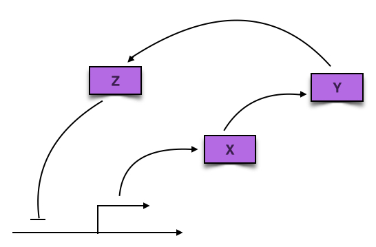
Figure 1: Goodwin Oscillator: a single gene

We now assume a continuous model where species diffuse in space. This example has been studied in [29]. The following system of PDEs, subject to Neumann boundary conditions, describe the evolution of $X$, $Y$, and $Z$ on $(0,1)\times[0,\infty)$:

$$\frac{\partial x}{\partial t} \;=\;\frac{a}{k+z}-b\;x+d_{1}\Delta x$$ (7)

$$\frac{\partial y}{\partial t} \;=\;{\alpha}\;x-\beta\;y+d_{2}\Delta y$$

$$\frac{\partial z}{\partial t} \;=\;\gamma\;y-\frac{\delta z}{k_{M}+z}+d_{3}\Delta z$$

Figure 2 provides plots of solutions $x$, $y$, and $z$ of (7), using the following parameter values from the textbook [47]:

$$a=150,\;k=1,\;b={\alpha}=\beta=\gamma=0.2,\;\delta=15,\;K_{M}=1.$$ (8)

which oscillate when there is no diffusion ($d_{1}=d_{2}=d_{3}=0$).

Figure 2: Goodwin Oscillator, no diffusion (parameters as in Eq. (8))

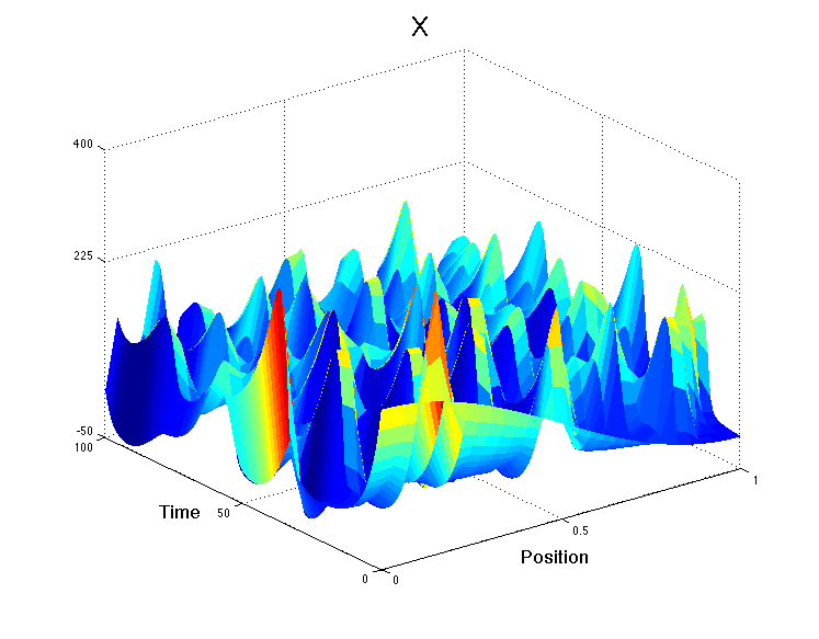
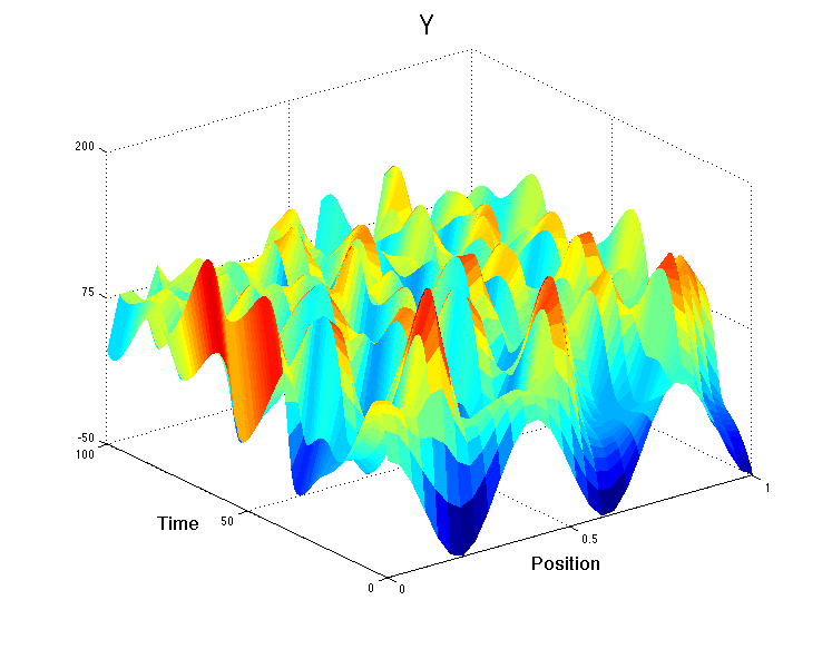
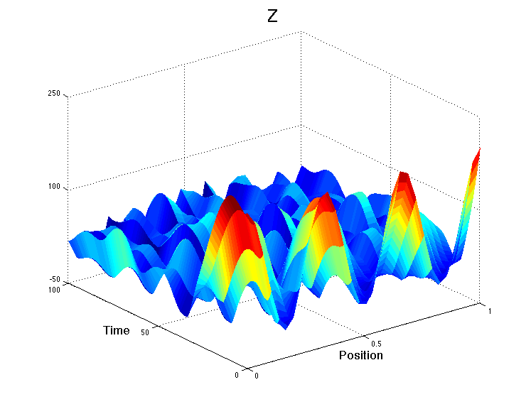
Figure 3 shows the spatially uniformity of the solutions of (7), for the same parameter values and initial conditions as in Figure 2, when ${2.2}/{\pi^{2}}<d_{1}$, $d_{1}=0.3$, and $d_{2}=d_{3}=0$.

In this work we provide a condition for synchronization when only $X$ diffuses, i.e. the diffusion matrix is $D=\mbox{diag}\,(d_{1},0,0)$. We will get back to this example later in Section 4, Remark 9.

Figure 3: Goodwin Oscillator, X diffuses (parameters as in Eq. (8))

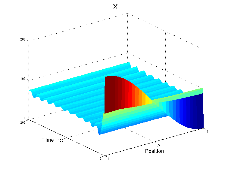
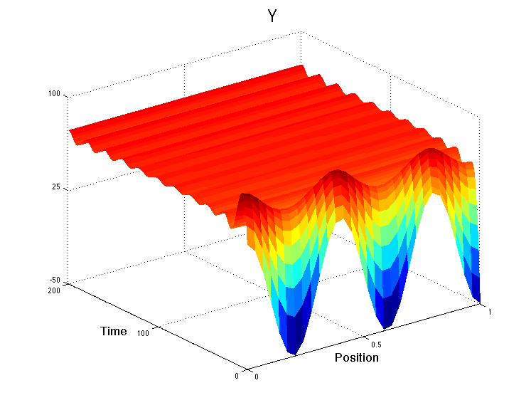
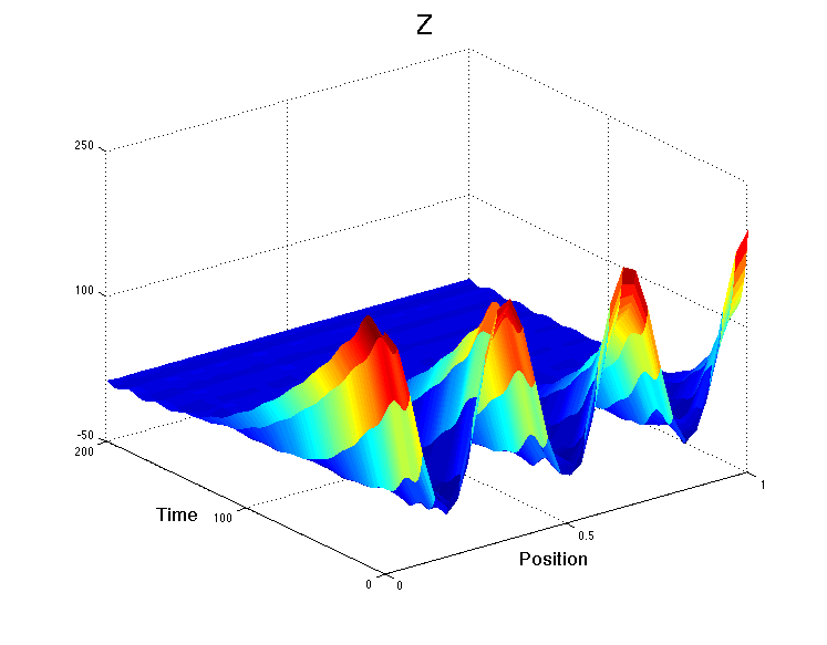
4 Convergence to uniform solutions in PDEs

In this section we review the existing results for synchronization and state and prove the new result.

We study reaction-diffusion PDE systems of the general form:

$$\frac{\partial u_{1}}{\partial t}(\omega,t) =F_{1}(u(\omega,t),t)+d_{1}\Delta u_{1}(\omega,t)$$

$$\vdots$$

$$\frac{\partial u_{n}}{\partial t}(\omega,t) =F_{n}(u(\omega,t),t)+d_{n}\Delta u_{n}(\omega,t)$$

which can be written as the following closed form:

$$\frac{\partial u}{\partial t}(\omega,t)=F_{t}(u(\omega,t))+D\Delta u(\omega,t)$$ (9)

subject to the Neumann boundary condition:

$$\frac{\partial u_{i}}{\partial\mathbf{n}}(\xi,t)=0\quad\forall\xi\in\partial\Omega,\;\;\forall t\in[0,\infty),\;\;\forall i=1,\ldots,n,$$ (10)

or subject to the Dirichlet boundary condition:

$$u_{i}(\xi,t)=0\quad\forall\xi\in\partial\Omega,\;\;\forall t\in[0,\infty),\;\;\forall i=1,\ldots,n,$$ (11)

where

• $F_{t}(x)=F(x,t)$ and $F\colon V\times[0,\infty)\to{\mathbb{R}}^{n}$ is a (globally) Lipschitz vector field with components $F_{i}$:

  $$F(x,t)\;=\;(F_{1}(x,t),\cdots,F_{n}(x,t))^{T},$$

  for some functions $F_{i}\colon V\times[0,\infty)\to{\mathbb{R}}$, where $V$ is a convex subset of ${\mathbb{R}}^{n}$.

• $D=\mbox{diag}\,(d_{1},\ldots,d_{n})$ with $d_{i}\geq 0$, and $d_{j}>0$ for some $j$, which we call the diffusion matrix.

• $\Omega$ is a bounded domain in ${\mathbb{R}}^{m}$ with smooth boundary $\partial\Omega$ and outward normal $\mathbf{n}$.

• $\displaystyle\frac{\partial u}{\partial\mathbf{n}}=\left(\displaystyle\frac{\partial u_{1}}{\partial\mathbf{n}},\ldots,\displaystyle\frac{\partial u_{n}}{\partial\mathbf{n}}\right)^{T}$.

In biology, a PDE system of this form describes individuals (particles, chemical species, etc.) of $n$ different types, with respective abundances $u_{i}(\omega,t)$ at time $t$ and location $\omega\in\Omega$, that can react instantaneously, guided by the interaction rules encoded into the vector field $F$, and can diffuse due to random motion.

Definition 4.

By a solution of the PDE

$$\frac{\partial u}{\partial t}(\omega,t)=F_{t}(u(\omega,t))+D\Delta u(\omega,t)$$

$$\frac{\partial u}{\partial\mathbf{n}}(\xi,t)=0\quad\forall\xi\in\partial\Omega,\;\;\forall t\in[0,\infty),$$

on an interval $[0,T)$, where $0<T\leq\infty$, we mean a function $u=(u_{1},\cdots,u_{n})^{T}$, with $u\colon\displaystyle\bar{\Omega}\times[0,T)\to V$, such that:

1. for each $\omega\in\bar{\Omega}$, $u(\omega,\cdot)$ is continuously differentiable;

2. for each $t\in[0,T)$, $u(\cdot,t)$ is in $\mathbf{Y}^{(n)}_{V}$, where

   $${\mathbf{Y}^{(n)}_{V}}\;=\;\left\{\begin{array}[]{c}\displaystyle v\colon\bar{\Omega}\to V,\quad v=(v_{1},\cdots,v_{n}),\\ v_{i}\in C^{2}_{{\mathbb{R}}}\left(\bar{\Omega}\right),\quad\displaystyle\frac{\partial v_{i}}{\partial\mathbf{n}}(\xi)=0,\;\forall\xi\in\partial\Omega,\;\;\forall i\end{array}\right\}$$

   and $C^{2}_{{\mathbb{R}}}\left(\bar{\Omega}\right)$ is the set of twice continuously differentiable functions $\bar{\Omega}\to{\mathbb{R}}$; and

3. for each $\omega\in\bar{\Omega}$, and each $t\in[0,T)$, $u$ satisfies the above PDE.

Definition 5.

By a solution of the PDE

$$\frac{\partial u}{\partial t}(\omega,t)=F_{t}(u(\omega,t))+D\Delta u(\omega,t)$$

$$u(\xi,t)=0\quad\forall\xi\in\partial\Omega,\;\;\forall t\in[0,\infty),$$

on an interval $[0,T)$, where $0<T\leq\infty$, we mean a function $u=(u_{1},\cdots,u_{n})^{T}$, with $u\colon\displaystyle\bar{\Omega}\times[0,T)\to V$, such that:

1. for each $\omega\in\bar{\Omega}$, $u(\omega,\cdot)$ is continuously differentiable;

2. for each $t\in[0,T)$, $u(\cdot,t)$ is in $\mathbf{Y}^{(d)}_{V}$, where

   $$\mathbf{Y}^{(d)}_{V}\;=\;\left\{\begin{array}[]{c}\displaystyle v\colon\bar{\Omega}\to V,\quad v=(v_{1},\cdots,v_{n}),\\ v_{i}\in C^{2}_{{\mathbb{R}}}\left(\bar{\Omega}\right),\quad\displaystyle v_{i}(\xi)=0,\;\forall\xi\in\partial\Omega,\;\;\forall i\end{array}\right\}$$

   and $C^{2}_{{\mathbb{R}}}\left(\bar{\Omega}\right)$ is the set of twice continuously differentiable functions $\bar{\Omega}\to{\mathbb{R}}$; and

3. for each $\omega\in\bar{\Omega}$, and each $t\in[0,T)$, $u$ satisfies the above PDE.

Under the additional assumptions that $F(x,t)$ is twice continuously differentiable with respect to $x$ and continuous with respect to $t$, theorems on existence and uniqueness for PDEs such as (9) can be found in standard references, e.g. [56, 57]. One must impose appropriate conditions on the vector field, on the boundary of $V$, to insure invariance of $V$. Convexity of $V$ insures that the Laplacian also preserves $V$. Since we are interested here in estimates relating pairs of solutions, we will not deal with existence and well-posedness. Our results will refer to solutions already assumed to exist.

Let $Q=\mbox{diag}\,(q_{1},\ldots,q_{n})$ be a positive diagonal matrix and $1\leq p\leq\infty$. Let

$$V_{p}\;:=\;(V,\|\cdot\|_{p,Q})$$ (12)

be a normed space, where for any $x=(x_{1},\cdots,x_{n})^{T}\in{\mathbb{R}}^{n}$, $\|x\|_{p,Q}$ is defined as follows:

$$\|x\|_{p,Q}\;=\;\left(\sum_{i=1}^{n}q_{i}^{p}\left|x_{i}\right|^{p}\right)^{\frac{1}{p}} 1\leq p<\infty$$ (13)

$$\|x\|_{\infty,Q}\;=\;\max_{1\leq i\leq n}q_{i}\left|x_{i}\right| p=\infty.$$

In this section, by $M_{V_{p}}[\cdot]$ or $M_{p,Q}[\cdot]$, we mean (lub) logarithmic Lipschitz constant induced by $\|\cdot\|_{p,Q}$ on $V$.

Definition 6.

We say that the reaction diffusion PDE (9) is contractive, if for any two solutions $u,v$ of (9), subject to the Neumann or Dirichlet boundary condition, $\|(u-v)(\cdot,t)\|\to 0$ as $t\to\infty$.

Definition 7.

We say that the reaction diffusion PDE (9) synchronizes, if for any solution $u$ of (9), subject to the Neumann or Dirichlet boundary condition, there exists $\bar{u}(t)$ such that $\|u(\cdot,t)-\bar{u}(t)\|\to 0$ as $t\to\infty$, or equivalently $\|\nabla u(\cdot,t)\|\to 0$ as $t\to\infty$.

The following theorem, from [49], provides a sufficient condition for contractivity of the reaction diffusion PDE (9) subject to the Neumann boundary condition (10). Then, in Remark 6 below, we show that how contractivity of the reaction diffusion PDE implies synchronization.

Theorem 1.

Consider the reaction diffusion PDE (9) subject to the Neumann boundary condition (10). Let $c=\displaystyle\sup_{t\in[0,\infty)}M_{p,Q}[F_{t}]$ for some $1\leq p\leq\infty$, and some positive diagonal matrix $Q$. Then for every two solutions $u,v$ of the PDE (9) subject to the Neumann boundary condition (10) and all $t\in[0,T)$:

$$\left\|u(\cdot,t)-v(\cdot,t)\right\|_{p,Q}\leq e^{ct}\left\|u(\cdot,0)-v(\cdot,0)\right\|_{p,Q}.$$

Remark 6.

Under the conditions of Theorem 1, if $c<0$, any solution $u$ of the PDE (9) with $u({\omega},0)=u_{0}({\omega})$ exponentially converges to the spatially uniform solution $\bar{u}(t)$ which is itself the solution of the following ODE system:

$$\dot{x} =F(x,t),$$ (14)

$$x(0) =\frac{1}{\left|\Omega\right|}\int_{\Omega}u_{0}({\omega})\;d{\omega}.$$

But, note that the condition $c<0$ rules out any interesting non-equilibrium behavior. For instance in Goodwin’s oscillatory system, $c<0$ kills out the oscillation. So we look for a weaker condition than $c<0$, that guarantees spatial uniform convergence result (which is a weaker property than contraction) while keeps interesting non-equilibrium behavior, like oscillatory in Goodwin example.

Recall [58] that for any bounded, open subset $\Omega\subset\mathbb{R}^{m}$, there exists a sequence of positive eigenvalues $0\leq\lambda_{1}^{(n)}\leq\lambda_{2}^{(n)}\leq\ldots$ (going to $\infty$, superscript $(n)$ for Neumann) and a sequence of corresponding orthonormal eigenfunctions: $\phi_{1}^{(n)},\phi_{2}^{(n)},\ldots$ (defining a Hilbert basis of $L^{2}(\Omega)$) satisfying the following Neumann eigenvalue problem:

$$-\Delta\phi_{i}^{(n)}=\lambda_{i}^{(n)}\phi_{i}^{(n)} \Omega$$    in (15)

$$\nabla\phi_{i}^{(n)}\cdot\mathbf{n}=0 \partial\Omega$$    on

Note that the first eigenvalue is always zero, ${\lambda}_{1}=0$, and the corresponding eigenfunction is a nonzero constant ($\phi({\omega})=1/\sqrt{\left|\Omega\right|}$).

The following re-phasing of a theorem from [29], provides a sufficient condition on $F$ and $D$ using the Jacobian matrix of the reaction term and the second Neumann eigenvalue of the Laplacian operator on the given spatial domain to insure the convergence of trajectories, in this case to their space averages in weighted $L^{2}$ norms. The proof in [29] is based on the use of a quadratic Lyapunov function, which is appropriate for Hilbert spaces. We have translated the result to the language of contractions. (Actually, the result in [29] is stronger, in that it allows for non-diagonal diffusion and also non-diagonal weighting matrices $Q$, by substituting these assumptions by a commutativity type of condition.)

Theorem 2.

Consider the reaction-diffusion system (9). Let

$$c:=\displaystyle\sup_{(x,t)\in V\times[0,\infty)}M_{2,Q}\left[J_{F}(x,t)-\lambda_{2}^{(n)}D\right],$$

where $Q$ is a positive diagonal matrix. Then

$$\|u(\cdot,t)-\tilde{u}(t)\|_{2,Q}\;\leq\;e^{ct}\|u(\cdot,0)-\tilde{u}(0)\|_{2,Q}.$$ (16)

where $\tilde{u}(t)=\displaystyle\frac{1}{\left|\Omega\right|}\displaystyle\int_{\Omega}u({\omega},t)\;d{\omega}$.

Note that when $c<0$, the reaction-diffusion system (9) synchronize. As we discussed in the biochemical example earlier,

$$\sup_{(x,t)\in V\times[0,\infty)}M_{2,Q}\left[J_{F}(x,t)-\lambda_{2}^{(n)}D\right]\geq 0,$$

therefore, conditions given in [29] do not hold for the biochemical example.

A generalization of Theorem 2 to spatially-varying diffusion is given in [59].

We next prove an analogous result to Theorem 2 for any norm but restricted to the linear operators $F$, $F(u,t)=A(t)u$, where for any $t$, $A(t)\in{\mathbb{R}}^{n\times n}$.

Theorem 3.

For a given norm $\|\cdot\|$ in ${\mathbb{R}}^{n}$, consider the reaction-diffusion system (9), for a linear operator $F$. Let

$$c:=\displaystyle\sup_{(x,t)\in V\times[0,\infty)}M\left[J_{F}(x,t)-\lambda_{2}^{(n)}D\right],$$

where $M$ is the logarithmic norm induced by $\|\cdot\|.$ Then for any ${\omega}\in\Omega$ and any $t\geq 0$,

$$\|u({\omega},t)-\bar{u}(t)\| \leq\sum_{i\geq 2}\left\|{\alpha}_{i}(t)\phi_{i}({\omega})\right\|$$

$$\leq e^{ct}\sum_{i\geq 2}\left\|{\alpha}_{i}(0)\phi_{i}({\omega})\right\|.$$

where $\bar{u}(t)$ is the solution of the system (14) with $u_{0}({\omega})=u({\omega},0)$, and ${\alpha}_{i}(t)=\int_{\Omega}u({\omega},t)\phi_{i}^{(n)}({\omega})\;d{\omega}$. In particular, when $c<0$,

$$\|u({\omega},t)-\bar{u}(t)\|\to 0\quad\mbox{exponentially, as $t\to\infty$}.$$

Proof.

We first show that the solution of Equation (14), $\bar{u}$, is equal to $\tilde{u}(t)=\frac{1}{\left|\Omega\right|}\int_{\Omega}u({\omega},t)\;d{\omega}$. Note that both $\bar{u}$ and $\tilde{u}$ satisfy $\dot{x}=A(t)x$. In addition, by the definition, $\bar{u}(0)=\tilde{u}(0)=\frac{1}{\left|\Omega\right|}\int_{\Omega}u({\omega},0)\;d{\omega}$. Therefore, by uniqueness of the solutions of ODEs, $\bar{u}(t)=\tilde{u}(t)$. The solution $u({\omega},t)$ can be written as follows:

$$u({\omega},t)\;=\;\displaystyle\sum_{i\geq 1}\phi_{i}({\omega}){\alpha}_{i}(t)$$ (17)

where for any $t$, ${\alpha}_{i}(t)=\int_{\Omega}u({\omega},t)\phi_{i}({\omega})\;d{\omega}\in{\mathbb{R}}^{n}$ and $\phi_{i}$’s are the eigenfunctions of (15).

Claim $1$.

$$u({\omega},t)-\bar{u}(t)\;=\;\displaystyle\sum_{i\geq 2}{\alpha}_{i}(t)\phi_{i}^{(n)}({\omega}).$$ (18)

Using the expansion of $u$ as in (17), we have

$$u({\omega},t)-\bar{u}(t) = {\alpha}_{1}(t)\phi_{1}^{(n)}({\omega})-\bar{u}(t)+\displaystyle\sum_{i\geq 2}\phi_{i}^{(n)}({\omega}){\alpha}_{i}(t).$$

Multiplying both sides of the above equality by the constant eigenfunction $\phi_{1}$ and taking integral over $\Omega$, by orthonormality of $\phi_{i}$’s, we get:

$$\int_{\Omega}\left(u({\omega},t)-\bar{u}(t)\right)\;d{\omega}={\alpha}_{1}(t).$$

We showed that $\bar{u}(t)=\frac{1}{\left|\Omega\right|}\int_{\Omega}u({\omega},t)\;d{\omega}$, hence ${\alpha}_{1}(t)=0$. This proves Claim $1$.

Claim $2$. Fix ${\omega}\in\Omega$. Then for any $i\geq 1$,

$$\dot{{\alpha}}_{i}(t) = (A(t)-{\lambda}_{i}^{(n)}D){\alpha}_{i}(t).$$

Using the expansion of $u$ as in (17) and after omitting the arguments ${\omega},t$ for simplicity, we have:

$$\displaystyle\sum_{i\geq 1}\dot{{\alpha}_{i}}\phi_{i}^{(n)} = \dot{u}=A(t)u+D\Delta u$$

$$= A(t)\left(\displaystyle\sum_{i\geq 1}{\alpha}_{i}\phi_{i}^{(n)}\right)+D\Delta\left(\displaystyle\sum_{i\geq 1}{\alpha}_{i}\phi_{i}^{(n)}\right)$$

$$= \displaystyle\sum_{i\geq 1}\left(A(t)-{\lambda}_{i}^{(n)}D\right){\alpha}_{i}\phi_{i}^{(n)}.$$

Multiplying both sides of the above equality by $\phi_{i}$ and taking integral over $\Omega$, by orthonormality of $\phi_{i}$’s we get:

$$\dot{{\alpha}}_{i}(t)\;=\;(A(t)-{\lambda}_{i}^{(n)}D){\alpha}_{i}(t).$$

This proves Claim $2$.

If for any $t$, $M\left[A(t)-\lambda_{2}^{(n)}D\right]\leq c$, then for any $t$ and any $i>2$, $M\left[A(t)-\lambda_{i}^{(n)}D\right]\leq c$ too. Then by Claim $2$ and Lemma 3:

$$\|{\alpha}_{i}(t)\|\leq e^{ct}\|{\alpha}_{i}(0)\|.$$ (19)

Using the above inequality and triangle inequality in Equation (18), for any ${\omega}\in\Omega$ and any $t$, we get the following inequality:

$$\|u({\omega},t)-\bar{u}(t)\| \leq \displaystyle\sum_{i\geq 2}\left\|{\alpha}_{i}(t)\phi_{i}^{(n)}({\omega})\right\|$$

$$\leq e^{ct}\displaystyle\sum_{i\geq 2}\left\|{\alpha}_{i}(0)\phi_{i}^{(n)}({\omega})\right\|.$$

Specifically, when $c<0$, $\|u({\omega},t)-\bar{u}(t)\|\to 0$, exponentially as $t\to\infty$. ∎

We next prove an analogues result to Theorem 1 (restricted to $p=1$), for reaction diffusion PDE (9) subject to the Dirichlet boundary condition (11).

Recall [58] that for any bounded, open subset $\Omega\subset\mathbb{R}^{m}$, there exists a sequence of positive eigenvalues $0<\lambda^{(d)}_{1}\leq\lambda^{(d)}_{2}\leq\ldots$ (going to $\infty$, superscript $(d)$ for Dirichlet) and a sequence of corresponding orthonormal eigenfunctions: $\phi^{(d)}_{1},\phi^{(d)}_{2},\ldots$ (defining a Hilbert basis of $L^{2}(\Omega)$) satisfying the following Dirichlet eigenvalue problem:

$$-\Delta\phi^{(d)}_{i} =\lambda^{(d)}_{i}\phi^{(d)}_{i}\quad\mbox{in $\Omega$}$$ (20)

$$\phi^{(d)}_{i} =0\quad\mbox{on $\partial\Omega$}.$$

Let us assume that $\Omega$ is a connected open set. Then the first eigenvalue ${\lambda}^{(d)}_{1}$ is simple and the first eigenfunction $\phi^{(d)}_{1}$ has a constant sign on $\Omega$. Without loss of generality, $\phi^{(d)}_{1}$ can be assumed to be everywhere positive on $\Omega$.

Let

$${Y^{(d)}}\;:=\;\left\{v\colon\bar{\Omega}\to{\mathbb{R}}^{n},\;v\in\left(C_{{\mathbb{R}}}^{2}\left(\bar{\Omega}\right)\right)^{n},\;v(\xi)=0,\;{\xi\in\partial\Omega}\right\}.$$

Then, for any $v=\left(v_{1},\cdots,v_{n}\right)^{T}\in Y^{(d)}$, $v_{i}$ can be written as follows:

$$v_{i}\;=\;\displaystyle\sum_{k=1}^{\infty}\langle v_{i},\phi^{(d)}_{k}\rangle\;\phi^{(d)}_{k},$$ (21)

where $\langle v_{i},\phi^{(d)}_{k}\rangle=\displaystyle\int_{\Omega}v_{i}\;\phi^{(d)}_{k}.$

Now consider the following weighted norm on $Y^{(d)}$:

For $Q=\mbox{diag}\,(q_{1},\ldots,q_{n})$, a positive diagonal matrix, and $\phi=\phi^{(d)}_{1}\geq 0$, we define

$$\|v\|_{1,\phi,Q}\;:=\;\displaystyle\sum_{i=1}^{n}q_{i}\displaystyle\int_{\Omega}\phi({\omega})\left|v_{i}({\omega})\right|\;d{\omega},\quad\mbox{$v=(v_{1},\ldots,v_{n})^{T}$},$$ (22)

and let

$${Y^{(d)}_{1,\phi}}:=\left(Y^{(d)},\|\cdot\|_{1,\phi,Q}\right).$$ (23)

In this section, by $M_{Y^{(d)}_{1,\phi}}[\cdot]$, we mean the (lub) logarithmic Lipschitz constant induced by $\|\cdot\|_{1,\phi,Q}$ on $Y^{(d)}$.

Now we state and prove the following theorem which provides sufficient condition for contractivity of the reaction diffusion PDE (9) subject to the Dirichlet boundary condition (11):

Theorem 4.

Consider the reaction diffusion PDE (9) subject to the Dirichlet boundary condition (11). Let

$$c_{1}=\displaystyle\sup_{(x,t)}M_{V_{1}}\left[J_{F_{t}}(x)-{\lambda}^{(d)}_{1}D\right],$$

where $M_{V_{1}}$ is the logarithmic norm induced by $Q$-weighted $L^{1}$ norm for a positive diagonal matrix $Q$ on $V$, and ${\lambda}_{1}^{(d)}$ is the first Dirichlet eigenvalue of $-\Delta$ on $\Omega$. Let $u(\omega,t)$ and $v(\omega,t)$ be two solutions of (9) and (11). Then

$$\|(u-v)(\cdot,t)\|_{1,\phi,Q}\leq e^{c_{1}t}\|(u-v)(\cdot,0)\|_{1,\phi,Q}$$ (24)

where $\phi=\phi^{(d)}_{1}\geq 0$ is the eigenfunction corresponding to ${\lambda}^{(d)}_{1}$.

To prove Theorem 4, we need the following lemmas:

Lemma 4.

Let $\Omega$ be an open subset of ${\mathbb{R}}^{m}$. Let $\mathcal{A}$ denote an $n\times n$ diagonal matrix of operators on $Y^{(d)}$ with the operators $d_{i}\Delta$ on the diagonal. Let $\Lambda^{(d)}$ denote an $n\times n$ diagonal matrix of operators on $Y^{(d)}$ with operators

$$\Lambda_{i}^{(d)}(\psi)({\omega}):={\lambda}_{1}^{(d)}d_{i}\psi_{i}({\omega})$$

on the diagonal. Then, for $p=1$,

$$M^{+}_{Y^{(d)}_{1,\phi}}\left[\mathcal{A}+\Lambda^{(d)}\right]=0,$$ (25)

where $M^{+}_{Y^{(d)}_{1,\phi}}$ is induced by $\|\cdot\|_{1,\phi,Q}$.

See Appendix for the proof.

Lemma 5.

Let $G\colon{\mathbb{R}}^{n}\to{\mathbb{R}}^{n}$ be a (globally) Lipschitz function and define $\hat{G}\colon Y^{(d)}\to{\mathbb{R}}^{n}$ as follows:

$$\hat{G}(u)({\omega}):=G(u({\omega})).$$

Then,

$$M^{+}_{Y^{(d)}_{1,\phi}}[\hat{G}]\leq M^{+}_{V_{1}}[G]=\displaystyle\sup_{x}M^{+}_{V_{1}}[J_{G}(x)].$$ (26)

In [49, Lemma 7], we proved a simpler version of this lemma, namely, we showed that Equation (26) holds when $\phi=1$, i.e. there is no weighted norm in the space. One can modify the proof of [49, Lemma 7] to get Equation (26). See Appendix for more details.

Proof of Theorem 4. Suppose that $u$ is a solution of Equation (9) defined on $\Omega\times[0,T)$. Note that for any $t$, $u(\cdot,t)\in Y^{(d)}$.

Define $\hat{u}\colon[0,T)\to Y^{(d)}$ by

$$\hat{u}(t)({\omega})\;:=\;u({\omega},t).$$

Also define $\mathcal{H}_{t}\colon Y^{(d)}\to{\mathbb{R}}^{n}$ as follows: for any $\psi\in Y^{(d)}$ and any ${\omega}\in\Omega$:

$$\mathcal{H}_{t}(\psi)({\omega})\;:=\;F_{t}(\psi({\omega})).$$

Let $\mathcal{A}$ denote an $n\times n$ diagonal matrix of operators on $Y^{(d)}$ with the operators $d_{i}\Delta$ on the diagonal. Then

$$\frac{\partial\hat{u}}{\partial t}(t)\;=\;\left(\mathcal{H}_{t}+\mathcal{A}\right)\left(\hat{u}(t)\right).$$ (27)

Suppose $u$ and $v$ are two solutions of Equation (9). By Lemma 3, we have:

$$D^{+}\|(\hat{u}-\hat{v})(t)\|_{1,\phi,Q} \leq M^{+}_{Y^{(d)}_{1,\phi}}[\mathcal{H}_{t}+\mathcal{A}]\|(\hat{u}-\hat{v})(t)\|_{1,\phi,Q}.$$ (28)

Let $\Lambda^{(d)}$ be as in Lemma 4. By subadditivity of $M^{+}$, Proposition 2, Lemma 4 and Lemma 5, we have:

$$M^{+}_{Y^{(d)}_{1,\phi}}[\mathcal{H}_{t}+\mathcal{A}] \leq M^{+}_{Y^{(d)}_{1,\phi}}[\mathcal{H}_{t}-\Lambda^{(d)}]+M^{+}_{Y^{(d)}_{1,\phi}}[\mathcal{A}+\Lambda^{(d)}]$$ (29)

$$\leq M^{+}_{Y^{(d)}_{1,\phi}}\left[\mathcal{H}_{t}-\Lambda^{(d)}\right]$$

$$\leq\sup_{x\in V}M_{V_{1}}\left[J_{F_{t}}(x)-{\lambda}_{1}^{(d)}D\right]$$

$$\leq\sup_{t\in[0,T)}\sup_{x\in V}M_{V_{1}}\left[J_{F_{t}}(x)-{\lambda}_{1}^{(d)}D\right]$$

$$=c_{1}.$$

By (28), (29), and Lemma 3, we get:

$$\|(\hat{u}-\hat{v})(t)\|_{1,\phi,Q}\leq e^{c_{1}t}\|(\hat{u}-\hat{v})(0)\|_{1,\phi,Q}.$$

In terms of the PDE (9), this last estimate can be equivalently written as:

$$\|(u-v)(\cdot,t)\|_{1,\phi,Q}\leq e^{c_{1}t}\|(u-v)(\cdot,0)\|_{1,\phi,Q}.$$

∎

Note that unlike in Neumann boundary problems, one cannot conclude synchronization from contraction in the Dirichlet boundary problems unless for any $t$, $F(0,t)=0$:

Corollary 1.

Under the conditions of Theorem 4, if $F(0,t)=0$, then $v=0$ is a uniformly spatial solution of Equations (9) and (11), and therefore, for any solution $u$ of Equations (9) and (11),

$$\|u(\cdot,t)\|_{1,\phi,Q}\leq e^{c_{1}t}\|u(\cdot,0)\|_{1,\phi,Q},$$

Hence, when $c_{1}<0$, the PDE system synchronizes.

The following theorem provides a sufficient condition for synchronization of reaction diffusion systems subject to the Neumann boundary condition restricted to $1D$ space and $p=1$. The proof is based on the results of Theorem 4.

Theorem 5.

Let $u(\omega,t)$ be a solution of

$$\frac{\partial u}{\partial t}(\omega,t)=F(u(\omega,t),t)+D\;\frac{\partial^{2}u}{\partial\omega^{2}}(\omega,t)\quad\mbox{on $(0,L)$}$$ (30)

$$\frac{\partial u}{\partial\omega}(0,t)\;=\;\frac{\partial u}{\partial\omega}(L,t)\;=\;0,$$

defined for all $t\in[0,T)$ for some $0<T\leq\infty$. In addition, assume that $u(\cdot,t)\in C^{3}(\Omega)$, for all $t\in[0,T)$. Let

$$c\;=\;\displaystyle\sup_{t\in[0,T)}\displaystyle\sup_{x\in V}M_{V_{1}}\left[J_{F_{t}}(x)-\displaystyle\frac{\pi^{2}}{L^{2}}D\right],$$

where $M_{V_{1}}$ is the logarithmic norm induced by $\|\cdot\|_{1,Q}$ for a positive diagonal matrix $Q$. Then for all $t\in[0,T)$:

$$\left\|\displaystyle\frac{\partial u}{\partial\omega}(\cdot,t)\right\|_{1,\phi,Q}\leq e^{ct}\left\|\displaystyle\frac{\partial u}{\partial\omega}(\cdot,0)\right\|_{1,\phi,Q},$$ (31)

where

$$\|\cdot\|_{1,\phi,Q}:=\left\|\sin(\pi{\omega}/L)(\cdot)\right\|_{1,Q}.$$

The significance of Theorem 5 lies in the fact that $\sin(\pi{\omega}/L)$ is nonzero everywhere in the domain (except at the boundary). In that sense, we have exponential convergence to uniform solutions in a weighted $L^{1}$ norm, the weights being specified in $V$ by the matrix $Q$ and in space by the function $\sin\left(\pi{\omega}/L\right)$.

Proof.

Suppose that $u$ is a solution of Equation (30) defined on $[0,L]\times[0,T)$. Let $v=\displaystyle\frac{\partial u}{\partial{\omega}}$, then by taking $\frac{\partial}{\partial{\omega}}$ in both sides of Equation (30), we get the following PDE:

$$\frac{\partial v}{\partial t}=J_{F_{t}}(u)v+D\Delta v,$$ (32)

subject to Dirichlet boundary condition: $v(0)=v(L)=0.$

For $\Omega=(0,L)$, the first Dirichlet eigenvalue is $\pi^{2}/L^{2}$ and a corresponding eigenfunction is $\sin(\pi{\omega}/L)$. Therefore, by Corollary 1,

$$\|{v}(\cdot,t)\|_{1,\phi,Q}\leq e^{ct}\|{v}(\cdot,0)\|_{1,\phi,Q},$$

where $c\;=\;\displaystyle\sup_{t\in[0,T)}\displaystyle\sup_{x\in V}M_{V_{1}}\left[J_{F_{t}}(x)-\displaystyle\frac{\pi^{2}}{L^{2}}D\right].$ ∎

Remark 7.

In the case of $\Omega=(0,L)$, ${\lambda}_{1}^{(d)}={\lambda}_{2}^{(n)}$.

Remark 8.

In the Biochemical model, we showed that there exists a positive diagonal matrix $Q$ such that

$$c:=\displaystyle\sup_{x\in V}M_{V}[J_{F}(x)]<0,$$

with norm $\|\cdot\|_{1,Q}$ on $V$. This condition implies that any solution of (4) converges to a uniform solution with rate $c$ (Remark 6). Next, we show that by Theorem 5, any solution of (4) converges to a uniform solution at a better rate than $c$:

By subadditivity of $M_{V}$, we have:

$$\sup_{x\in V}M_{V}[J_{F}(x)-\pi^{2}D]\leq\displaystyle\sup_{x\in V}M_{V}[J_{F}(x)]-\pi^{2}d,\quad\mbox{where $d=\min\{d_{1},d_{2}\}$}.$$

Therefore, $c_{0}:=\displaystyle\sup_{x\in V}M_{V}[J_{F}(x)-\pi^{2}D]<c<0$. Hence, by Theorem 5, for any solution $u$ of (4):

$$\left\|\displaystyle\frac{\partial u}{\partial{\omega}}(\cdot,t)\right\|_{1,\phi,Q}\;\leq\;e^{c_{0}t}\;\left\|\displaystyle\frac{\partial u}{\partial{\omega}}(\cdot,0)\right\|_{1,\phi,Q},$$

where $\phi({\omega})=\sin(\pi{\omega}).$

Figure 4 indicates two different solutions of the Biochemical model, Equation (4), namely $(x_{1},y_{1})^{T}$ and $(x_{2},y_{2})^{T}$ on $\Omega=(0,2)$ for $z(t)=20(1+\sin(10t))$, and for the following set of parameters:

$$\delta=20,\;k_{1}=0.5,\;k_{2}=5,\;S_{Y}=0.1,\;d_{1}=0.001,\;d_{2}=0.1.$$

Also, in Figure 4, the difference between two solutions has been shown that goes to zero as expected.

Figure 4: Two different solutions of (4) and their difference.

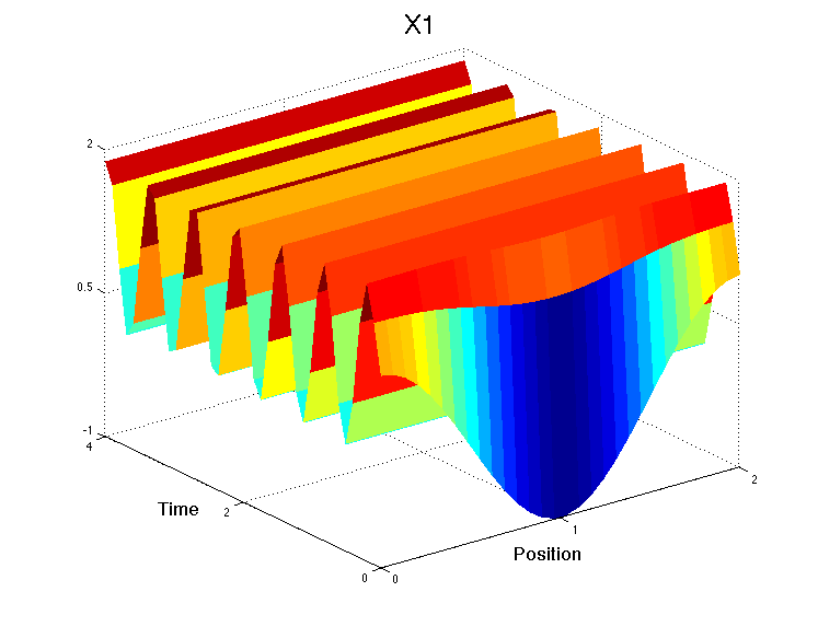
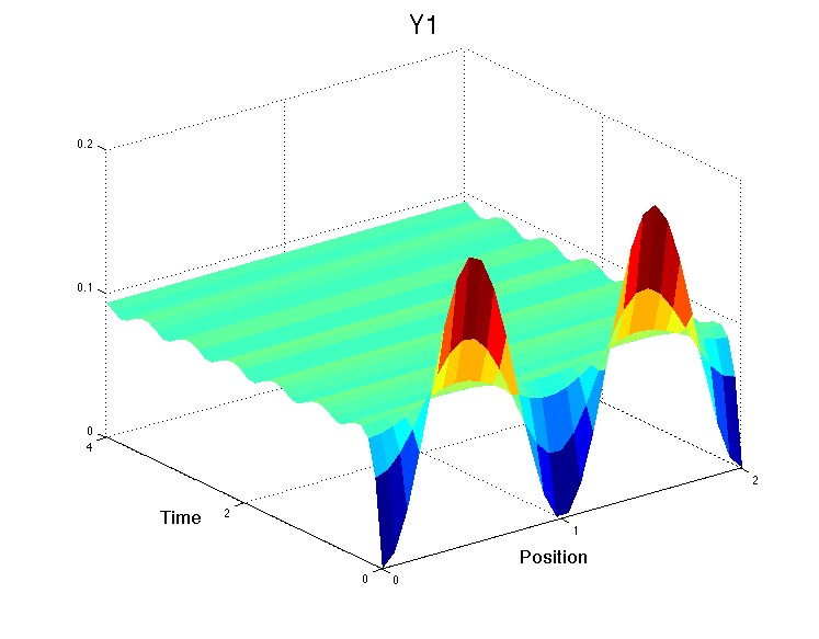
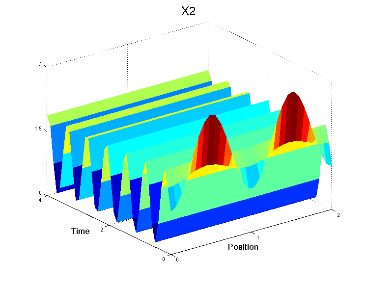
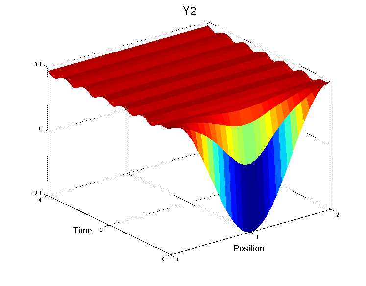
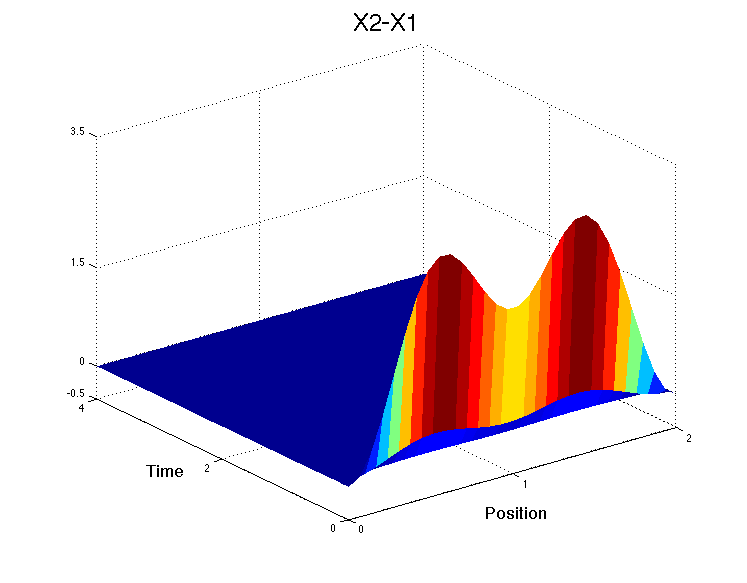
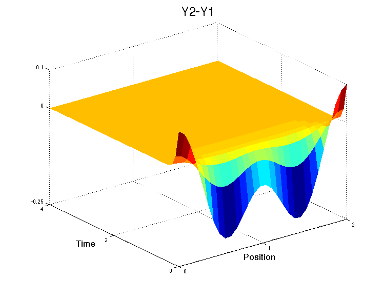
In the following remark w compare our result, Theorem 5, with the results in [29] and [60].

Remark 9.

Considering (7), in ([29], Equation 55), the following sufficient condition is given for synchronization:

$$\frac{{\alpha}\gamma a}{k(b+{\lambda}d_{1})({\beta}+{\lambda}d_{2}){\lambda}d_{3}}\;<\;4,$$ (33)

where ${\lambda}=\pi^{2}$.

A simple calculations show that for weighted matrix $Q=\mbox{diag}\,(1,12,11)$, and for $2.2/\pi^{2}<d_{1}$, and $d_{2}=d_{3}=0$,

$$\sup_{w=(x,y,z)^{T}}M_{1,Q}[J_{F}(w)-\pi^{2}D]<0.$$

Applying Theorem 5, we conclude that for ${2.2}/{\pi^{2}}<d_{1}$, and $d_{2}=d_{3}=0$, (7) synchronizes, meaning that solutions tend to uniform solutions.

Note that when $d_{3}=0$, one cannot apply (33) directly to get synchronization.

Figure 3 shows the spatially uniformity of the solutions of (7), for the same parameter values and initial conditions as in Figure 2, when ${2.2}/{\pi^{2}}<d_{1}$, and $d_{2}=d_{3}=0$.

In ([60], Equation 3), Othmer provides a sufficient condition for uniform behavior of the solutions of the reaction-diffusion (9) on $(0,L)$, subject to Neumann boundary conditions:

$$\sup_{w}\|J_{F}(w)\|<\pi^{2}/L^{2}\min\{d_{i}\}.$$ (34)

In Goodwin’s example (7), $\sup_{w}\|J_{F}(w)\|$ is positive and finite (the $\sup$ is taken at $z=0$), and $\min\{d_{i}\}=0$, hence (34) doesn’t hold and this condition is not applicable for this example.

5 Synchronization in a system of ODEs

In this section, we study a network of identical ODE models which are diffusively interconnected.

The state of the system will be described by a vector $x$ which one may interpret as a vector collecting the states $x_{i}$ (each of them itself possibly a vector) of identical “agents” which tend to follow each other according to a diffusion rule, with interconnections specified by an undirected graph. Another interpretation, useful in the context of biological modeling, is a set of chemical reactions among species that evolve in separate compartments (e.g., nucleus, cytoplasm, membrane, in a cell); then the $x_{i}$’s represent the vectors of concentrations of the species in each separate compartment.

In order to formally describe the interconnections, we use the following concepts in this section:

• For a fixed convex subset of ${\mathbb{R}}^{n}$, say $V$, $\tilde{F}\colon V^{N}\times[0,\infty)\to{\mathbb{R}}^{nN}$ is a function of the form:

  $$\tilde{F}(x,t)=\left(F(x_{1},t)^{T},\ldots,F(x_{N},t)^{T}\right)^{T},$$

  where $x=\left(x_{1}^{T},\ldots,x_{N}^{T}\right)^{T}$, with $x_{i}\in V$ for each $i$, and $F(\cdot,t):=F_{t}\colon V\to{\mathbb{R}}^{n}$ is a $C^{1}$ function.

• For any $x\in V^{N}$ we define $\left\|x\right\|_{p,Q}$ as follows:

  $$\left\|x\right\|_{p,Q}=\left\|\left(\|Qx_{1}\|_{p},\cdots,\|Qx_{N}\|_{p}\right)^{T}\right\|_{p},$$

  where $Q=\mbox{diag}\,{(q_{1},\ldots,q_{n})}$ is a positive diagonal matrix and $1\leq p\leq\infty$.

  With a slight abuse of notation, we use the same symbol for a norm in ${\mathbb{R}}^{n}$:

  $$\|x\|_{p,Q}:=\|Qx\|_{p}.$$

• $D=\mbox{diag}\,(d_{1},\ldots,d_{n})$ with $d_{i}\geq 0$, and $d_{j}>0$ for some $j$, which we call the diffusion matrix.

• $\mathcal{L}\in{\mathbb{R}}^{N\times N}$ is a symmetric matrix and $\mathcal{L}\mathbf{1}=0$, where $\mathbf{1}=(1,\ldots,1)^{T}$. We think of $\mathcal{L}$ as the Laplacian of a graph that describes the interconnections among component subsystems.

• $\otimes$ denotes the Kronecker product of two matrices.

Definition 8.

For any arbitrary graph $\mathcal{G}$ with the associated (graph) Laplacian matrix $\mathcal{L}$, any diagonal matrix $D$, and any $F\colon V\times[0,\infty)\to{\mathbb{R}}^{n}$, the associated $\mathcal{G}-$compartment system, denoted by $(F,\mathcal{G},D)$, is defined by

$$\dot{x}(t)=\tilde{F}(x(t),t)-(\mathcal{L}\otimes D)x(t),$$ (35)

where $x,\tilde{F},$ and $D$ are as defined above.

The “symmetry breaking” phenomenon of diffusion-induced, or Turing, instability refers to the case where a dynamic equilibrium $\bar{u}$ of the non-diffusing ODE system $\dot{x}=F(x,t)$ is stable, but, at least for some diagonal positive matrices $D$, the corresponding interconnected system (35) is unstable.

The following theorem (from [49]), shows that, for contractive reaction part $F$, no diffusion instability will occur, no matter what is the size of the diffusion matrix $D$.

Theorem 6.

Consider the system $(\ref{g-compartment})$. Let

$$c=\displaystyle\sup_{t\in[0,\infty)}M_{p,Q}[F_{t}],$$

where $M_{p,Q}$ is the (lub) logarithmic Lipschitz constant induced by the norm $\|\cdot\|_{p,Q}$ on ${\mathbb{R}}^{n}$ defined by $\|x\|_{p,Q}:=\|Qx\|_{p}$. Then for any two solutions $x,y$ of $(\ref{g-compartment})$, we have

$$\left\|x(t)-y(t)\right\|_{p,Q}\leq e^{ct}\left\|x(0)-y(0)\right\|_{p,Q}.$$

Remark 10.

Under the assumptions of Theorem 6, by Remark 5, if for any $t\geq 0$ and any $x$, $M_{p,Q}[J_{F}(x,t)]\leq c$, then

$$\left\|x(t)-y(t)\right\|_{p,Q}\leq e^{ct}\left\|x(0)-y(0)\right\|_{p,Q}.$$

Definition 9.

We say that the $\mathcal{G}-$compartment system (35) synchronizes, if for any solution $x=\left(x_{1}^{T},\ldots,x_{N}^{T}\right)^{T}$ of (35), and for all $i,j\in\{1,\ldots,N\}$, $(x_{i}-x_{j})(t)\to 0$ as $t\to\infty$.

An easy first result is as follows.

Proposition 3.

Under the assumptions of Theorem 6, if $c<0$, then the $\mathcal{G}-$compartment system (35) synchronizes.

Proof.

Note that $z(t):=\left(z_{1}(t),\ldots,z_{1}(t)\right)^{T}$ is a solution of (35), where $z_{1}(t)$ is a solution of $\dot{x}=F(x,t)$. By Theorem 6, if for any $t\geq 0$ and any $x$, $M_{p,Q}[J_{F}(x,t)]\leq c$, then for any solution $x(t)$ of (35),

$$\left\|x(t)-z(t)\right\|_{p,Q}\leq e^{ct}\left\|x(0)-z(0)\right\|_{p,Q}.$$

When $c<0$, $(x_{i}-z_{1})(t)\to 0$, hence $(x_{i}-x_{j})(t)\to 0$ as $t\to\infty$. ∎

In Proposition 3, we imposed a strong condition on $F$, which in turn leads to the very strong conclusion that all solutions should converge exponentially to a particular solution, no matter the strength of the interconnection (choice of diffusion matrix). A more interesting and challenging problem is to provide a condition that links the vector field, the graph structure, and the matrix $D$, so that interesting dynamical behaviors (such as oscillations in autonomous systems, which are impossible in contractive systems) can be exhibited by the individual systems, and yet the components synchronize. The following example illustrates this question.

An example: synchronous autonomous oscillators

We consider the following three-dimensional system (all variables are non-negative and all coefficients are positive):

$$\dot{x} \;=\;\frac{a}{k+z}-bx$$ (36)

$$\dot{y} \;=\;{\alpha}x-\beta y$$

$$\dot{z} \;=\;\gamma y-\frac{\delta z}{k_{M}+z}.$$

where $x,y,$ and $z$ are functions of $t$. This system is a variation ([55]) of a model, often called in mathematical biology the “Goodwin model,” that was proposed in order to describe a generic model of an oscillating autoregulatory gene, and its oscillatory behavior has been well-studied [54]. It is sketched in Fig. 1. In Goodwin’s original formulation, $X$ is the mRNA transcribed from a given gene, $Y$ an enzyme translated from this mRNA, and $Z$ a metabolite whose production is catalyzed by $Y$. It is assumed that $Z$, in turn, can inhibits the expression of the original gene. However, many other interpretations are possible. Fig. 5(a), shows non-synchronized oscillatory solutions of (36) for $6$ different initial conditions, using the following parameter values from the textbook [47]:

$$a=150,\;k=1,\;b={\alpha}=\beta=\gamma=0.2,\;\delta=15,\;K_{M}=1.$$

Fig. 5(b) shows the solutions of the same system ($6$ compartments, with the same initial conditions as in Fig. 5(a)) that are now interconnected diffusively by a linear graph in which only $X$ diffuses, that is, $D=\mbox{diag}\,(d,0,0)$. The following system of ODEs describes the evolution of the full system: (in all equations, $i=1,\ldots,N$):

$$\dot{x}_{i} \;=\;\frac{a}{k+z_{i}}-b\;x_{i}\;+d\left(x_{i-1}-2x_{i}+x_{i+1}\right)$$

$$\dot{y}_{i} \;=\;{\alpha}\;x_{i}-\beta\;y_{i}$$

$$\dot{z}_{i} \;=\;\gamma\;y_{i}-\frac{\delta z_{i}}{k_{M}+z_{i}}$$

where for convenience we are writing $x_{0}=x_{1}$ and $x_{N}=x_{N+1}$. In Fig. 5(c) we show solutions of the same system ($6$ compartments with the same initial conditions as in Fig. 5(a)) that are now interconnected, with the same $D$, by a complete graph. Observe that the second and “more connected” graph structure (reflected, as discussed in the magnitude of its second Laplacian eigenvalue, which is used in the conditions discussed below) leads to much faster synchronization.

Figure 5: Goodwin Oscillator

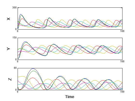
(a) $6$ isolated compartments

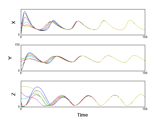
(b) Linear interconnection

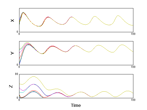
(c) Complete interconnection

Synchronization conditions based on contractions

In this section, we discuss several matrix measure based conditions that guarantee synchronization of ODE systems; for additional results, see [10, 30, 31, 12, 61].

We will use ideas from spectral graph theory, see for example [62]. Recall that a Laplacian matrix $\cal{L}$, with eigenvalues ${\lambda}_{1}\leq\ldots\leq{\lambda}_{N}$, is always positive semi-definite ($0={\lambda}_{1}\leq\ldots\leq{\lambda}_{N}$). In a connected graph, ${\lambda}_{1}$ is the only zero eigenvalue and $v_{1}=(1,\ldots,1)^{T}$ is the unique corresponding eigenvector (up to a constant). The second smallest eigenvalue, ${\lambda}_{2}$, is called the algebraic connectivity of the graph. This number helps quantify the “how connected” the graph is; for example, a complete graph is “more connected” than a linear graph with the same number of nodes, and this is reflected in the fact that the second eigenvalue of the Laplacian matrix of a complete graph (${\lambda}_{2}=N$) is larger that the second eigenvalue of the Laplacian matrix of a line graph (${\lambda}_{2}=4\sin^{2}\left(\pi/2N\right)$).

Consider a $\mathcal{G}-$compartment system, $(F,\mathcal{G},D)$, where $\mathcal{G}$ is any arbitrary graph. The following re-phasing of a theorem from [29], provides sufficient conditions on $F$ and $D$, based upon contractions with respect to $L^{2}$ norms, that guarantee synchrony of the associated $\mathcal{G}-$compartment system. We have translated the result to the language of contractions. (Actually, the result in [29] is stronger, in that it allows for certain non-diagonal diffusion and also certain non-diagonal weighting matrices $Q$, by substituting these assumptions by a commutativity type of condition.)

Theorem 7.

Consider a $\cal{G}-$compartment as defined in Equation (35) and suppose that $V\subseteq{\mathbb{R}}^{n}$ is convex. For a given diagonal positive matrix $Q$, let

$$c\;:=\;\displaystyle\sup_{(x,t)}M_{2,Q}[J_{F}(x,t)-{\lambda}_{2}D].$$ (37)

Then for every forward-complete solution $x$ that remains in $V$, the following inequality holds:

$$\left\|\left(\begin{array}[]{c}x_{1}-\bar{x}\\ \vdots\\ x_{N}-\bar{x}\end{array}\right)(t)\right\|_{2,I\otimes Q}\;\leq\;e^{ct}\left\|\left(\begin{array}[]{c}x_{1}-\bar{x}\\ \vdots\\ x_{N}-\bar{x}\end{array}\right)(0)\right\|_{2,I\otimes Q},$$

where $\bar{x}=(x_{1}+\ldots+x_{N})/N$.

In particular, if $c<0$, then for any pair $i,j\in\{1,\ldots,N\}$, $(x_{i}-x_{j})(t)\to 0$ exponentially as $t\to\infty$.

Recall that a directed incidence matrix of a graph with $N$ nodes and $m$ edges, is an $N\times m$ matrix $E$ which is defined as follows, for any fixed ordering of nodes and edges: The $(i,j)-$entry of $E$ is $0$ if vertex $i$ and edge $e_{j}$ are not incident, and otherwise, it is $1$ if $e_{j}$ originates at vertex $i$, and $-1$ if $e_{j}$ terminates at vertex $i$. In addition, the (graph) Laplacian matrix $\mathcal{L}$ of $\mathcal{G}$, is equal to $EE^{T}$. Observe that $E^{T}\mathcal{L}=E^{T}(EE^{T})=(E^{T}E)E^{T}$, so this means that $K:=E^{T}E$ satisfies

$$E^{T}\mathcal{L}=KE^{T}\,.$$ (38)

Note that $E^{T}E$ is called edge Laplacian of $\mathcal{G}$. If $E^{T}E$ is nonsingular (e.g. in linear graphs), then $K=E^{T}E$ is the unique matrix satisfying (38). However, in general, $K$ is not necessarily unique. For example, suppose that $\mathcal{G}$ is a complete graph. Then $E^{T}EE^{T}=NE^{T}$ (see the proof of Proposition 6). So one can pick $K=NI$, where $I$ is the identity matrix. Since $E^{T}E\neq NI$, in a complete graph, this gives an alternative choice of $K$.

The following theorem, provides a sufficient condition on $F,D,$ and $\mathcal{G}$ that guarantees synchrony of the associated $\mathcal{G}-$compartment system in any norm.

Theorem 8.

Consider a $\mathcal{G}-$compartment system, $(F,\mathcal{G},D)$, where $\mathcal{G}$ is an arbitrary graph of $N$ nodes and $m$ edges, and a norm $\|\cdot\|$ on ${\mathbb{R}}^{nm}$. Let $E$ be a directed incidence matrix of $\mathcal{G}$, and pick any $m\times m$ matrix $K$ satisfying (38). Denote:

$$c\;:=\;\displaystyle\sup_{(w,t)}M\left[J(w,t)-K\otimes D\right],$$ (39)

where $M$ is the logarithmic norm induced by $\|\cdot\|$, and $J(w,t)$ is defined as follows:

$$J(w,t)=\mbox{diag}\,\left(J_{F}(w_{1},t),\ldots,J_{F}(w_{m},t)\right),$$

where

$$w=\left(w_{1}^{T},\ldots,w_{m}^{T}\right)^{T}$$

and $J_{F}$ denotes the Jacobian of $F$. Then

$$\left\|\left(E^{T}\otimes I\right)x(t)\right\|\;\leq\;e^{ct}\left\|\left(E^{T}\otimes I\right)x(0)\right\|.$$

Note that $\left(E^{T}\otimes I\right)x$ is a column vector whose entries are the differences $x_{i}-x_{j}$, for each edge $e=\{i,j\}$ in $\mathcal{G}$. Therefore, if $c<0$, the system synchronizes.

Proof.

Assume that $x$ is a solution of

$$\dot{x}=\tilde{F}(x,t)-\left(\mathcal{L}\otimes D\right)x.$$

Let’s define $y$ as follows: for any $t$,

$$y(t):=\left(E^{T}\otimes I\right)x(t)=\left(\begin{array}[]{c}x_{i_{1}}-x_{j_{1}}\\ \vdots\\ x_{i_{m}}-x_{j_{m}}\end{array}\right),$$

where for $k=1,\ldots,m$, $x_{i_{k}}-x_{j_{k}}$ indicates the $k$th edge of $\cal{G}$, i.e., the difference between states associated to the two nodes that constitute the edge, and $I$ is the $n\times n$ identity matrix. Then, using the Kronecker product identity

$$(A\otimes B)(C\otimes D)=AC\otimes BD$$

for matrices $A,B,C,$ and $D$ of appropriate dimensions, we have:

$$\dot{y} =\left(E^{T}\otimes I\right)\dot{x}$$

$$=\left(E^{T}\otimes I\right)\left(\tilde{F}(x,t)-\left(\mathcal{L}\otimes D\right)x\right)$$

$$=\left(E^{T}\otimes I\right)\tilde{F}(x,t)-\left(E^{T}\mathcal{L}\otimes D\right)x$$

$$=\left(E^{T}\otimes I\right)\tilde{F}(x,t)-\left(KE^{T}\otimes D\right)x$$

$$=\left(E^{T}\otimes I\right)\tilde{F}(x,t)-\left(K\otimes D\right)\left(E^{T}\otimes I\right)x$$

$$=\left(E^{T}\otimes I\right)\tilde{F}(x,t)-\left(K\otimes D\right)y,$$

where

$$\left(E^{T}\otimes I\right)\tilde{F}(x,t)=\left(\begin{array}[]{c}F(x_{i_{1}},t)-F(x_{j_{1}},t)\\ \vdots\\ F(x_{i_{m}},t)-F(x_{j_{m}},t)\end{array}\right).$$

Now let $u$, $v$, and $G$ be as follows:

$$u:=\left(\begin{array}[]{c}x_{i_{1}}\\ \vdots\\ x_{i_{m}}\end{array}\right),v:=\left(\begin{array}[]{c}x_{j_{1}}\\ \vdots\\ x_{j_{m}}\end{array}\right),$$

$$G_{t}(u):=\left(\begin{array}[]{c}F(x_{i_{1}},t)\\ \vdots\\ F(x_{i_{m}},t)\end{array}\right)-\left(K\otimes D\right)\left(\begin{array}[]{c}x_{i_{1}}\\ \vdots\\ x_{i_{m}}\end{array}\right),$$

then

$$\dot{u}-\dot{v}=G_{t}(u)-G_{t}(v).$$

By Remark 5,

$$\|u(t)-v(t)\|\;\leq\;e^{ct}\|u(0)-v(0)\|,$$

where

$$c\;=\;\displaystyle\sup_{(w,t)}M\left[J_{G_{t}}(w)\right]\;=\;\displaystyle\sup_{(w,t)}M\left[J(w,t)-K\otimes D\right].$$

∎

The following corollary is already known, see [29], but we show here how it follows from Theorem 8 as a special case.

Corollary 2.

Consider a $\mathcal{G}-$compartment system, $(F,\mathcal{G},D)$, where $\mathcal{G}$ is a tree (graphs with no cycles) and denote

$$c\;:=\;\displaystyle\sup_{(w,t)}M_{2,Q}\left[J_{F}(w,t)-{\lambda}D\right],$$

where ${\lambda}$ is the smallest nonzero eigenvalue of the Laplacian of $\mathcal{G}$ and $Q$ is a positive diagonal matrix. Then

$$\left\|\left(E^{T}\otimes I\right)x(t)\right\|_{2,I\otimes Q} \leq e^{ct}\left\|\left(E^{T}\otimes I\right)x(0)\right\|_{2,I\otimes Q}.$$

where $I$ is the identity matrix of appropriate size and $E$ is a directed incidence matrix of $\mathcal{G}$.

We will need the following lemmas to prove Corollary 2.

Lemma 6.

[63] Let $\mathcal{G}$ be a connected directed graph with incidence matrix $E$ and edge Laplacian $\mathcal{K}=E^{T}E$ and (graph) Laplacian $\mathcal{L}=EE^{T}$. Then

1. The nonzero eigenvalues of $\mathcal{K}$ are equal to the nonzero eigenvalues of $\mathcal{L}$.

2. The null space of the edge Laplacian depends on the number of cycles in the graph. In particular, the null space of a tree is equal to $0$, i.e. all the eigenvalues are nonzero.

Lemma 7.

Let $A$ be a block diagonal matrix with matrices $A_{1},\ldots,A_{n}$ on its diagonal. Then for any $1\leq p\leq\infty$,

$$M_{p}[A]\leq\max\left\{M_{p}[A_{1}],\ldots,M_{p}[A_{n}]\right\}.$$

See the Appendix for the proof.

Proof of Corollary 2.

Let $K=E^{T}E$ and $J=\mbox{diag}\,\left(J_{F}(w_{1},t),\ldots,J_{F}(w_{m},t)\right)$, where $m$ is the number of edges of $\mathcal{G}$. By subadditivity of $M$,

$$M_{2,I\otimes Q}\left[J(w,t)-K\otimes D\right] \leq M_{2,I\otimes Q}\left[J(w,t)-{\lambda}I\otimes D\right]$$ (40)

$$\;+\;M_{2,I\otimes Q}\left[{\lambda}I\otimes D-K\otimes D\right]$$

We first show that the second term of the right hand side of the above inequality is zero. By Lemma 6, ${\lambda}$ is the smallest eigenvalue of the edge Laplacian, $E^{T}E$, so the largest eigenvalue of ${\lambda}I-K$ and hence $({\lambda}I-K)\otimes D$ is $0$. Therefore,

$$M_{2,I\otimes Q}[({\lambda}I-K)\otimes D] = M_{2}\left[\left(I\otimes Q\right)\left(({\lambda}I-K)\otimes D\right)\left(I\otimes Q^{-1}\right)\right]$$

$$= M_{2}\left[({\lambda}I-K)\otimes D\right]$$

$$= \mbox{largest eigenvalue of $({\lambda}I-K)\otimes D$}=0.$$

Next, we will show that the first term of the right hand side of Equation (40) is $\leq c$.

By Lemma 7,

$$M_{2,I\otimes Q}\left[J(w,t)-{\lambda}I\otimes D\right] \leq \max_{i}\left\{M_{2,Q}\left[J_{F}(w_{i},t)-{\lambda}D\right]\right\}.$$

By taking $\displaystyle\sup$ over all $w=(w_{1}^{T},\ldots,w^{T}_{m})^{T}$ and all $t\geq 0$, we get

$$\sup_{(w,t)}M_{2,I\otimes Q}\left[J(w,t)-K\otimes D\right]=\displaystyle\sup_{t}\sup_{x\in{\mathbb{R}}^{n}}M_{2,Q}\left[J_{F}(x,t)-{\lambda}D\right]=c.$$

Now by applying Theorem 8, we obtain the desired inequality.

∎

In the following section, we will see the application of Theorem 8 to complete graphs (Proposition 6) and linear graphs (Proposition 5) in any weighted $L^{p}$ norm, $1\leq p\leq\infty$.

We next specialize to the linear case, $F(x,t)=A(t)x$.

Theorem 9.

Consider a $\mathcal{G}-$compartment system, $(F,\mathcal{G},D)$, and suppose that $F(x,t)=A(t)x$, i.e.,

$$\dot{x}(t)\;=\;\left(I\otimes A(t)-\mathcal{L}\otimes D\right)x(t).$$ (41)

For a given arbitrary norm in ${\mathbb{R}}^{n}$, $\|\cdot\|$, suppose that

$$\sup_{t}M[A(t)-{\lambda}_{2}D]<0,$$

where ${\lambda}_{2}$ is the smallest nonzero eigenvalue of the Laplacian matrix $\mathcal{L}$ and $M$ is the logarithmic norm induced by $\|\cdot\|$. Then, for any $i,j\in\{1,\ldots,N\}$, $(x_{i}-x_{j})(t)\to 0$, exponentially as $t\to\infty.$

Proof.

Note that any solution $x$ of Equation (41) can be written as follows:

$$x(t)\;=\;\displaystyle\sum_{i=1,\ldots,N}\;\displaystyle\sum_{j=1,\ldots,n}c_{ij}(t)\;(v_{i}\otimes e_{j})$$

where $v_{i}$’s, $v_{i}\in{\mathbb{R}}^{N}$ are a set of orthonormal eigenvectors of $\mathcal{L}$ (that make up a basis for ${\mathbb{R}}^{N}$), corresponding to the eigenvalues ${\lambda}_{i}$’s of $\cal{L}$, where we assume that the eigenvalues are ordered, and ${\lambda}_{1}=0$, and the $e_{j}$’s are the standard basis of ${\mathbb{R}}^{n}$. In addition, $c_{ij}$’s are the coefficients that satisfy

$$\dot{C}(t)=\left(\begin{array}[]{ccc}A(t)-{\lambda}_{1}D&&\\ &\ddots&\\ &&A(t)-{\lambda}_{N}D\end{array}\right)C(t),$$

where $C=\left(c_{11},\ldots,c_{1n},\ldots,c_{N1},\ldots,c_{Nn}\right)^{T}$, with appropriate initial conditions. By the definition of $y$, $y=(E^{T}\otimes I)x$, we have

$$y(t) =\sum_{i=1,\ldots,N}\;\sum_{j=1,\ldots,n}c_{ij}(t)\;\left(E^{T}v_{i}\otimes e_{j}\right)$$

$$=\sum_{i=2,\ldots,N}\;\sum_{j=1,\ldots,n}c_{ij}(t)\;\left(E^{T}v_{i}\otimes e_{j}\right)$$

because $E^{T}v_{1}=0$ (where $v_{1}=(1/\sqrt{n})(1,\ldots,1)^{T}$). Therefore, if $\displaystyle\sup_{t}M[A(t)-{\lambda}_{2}D]<0$, then $\displaystyle\sup_{t}M[A(t)-{\lambda}_{i}D]<0,i=2,\ldots,N$, and by Lemma 3, the $c_{ij}(t)$’s, for $j\geq 2$, and hence also $y(t)$, converge to $0$ exponentially as $t\to\infty$. ∎

5.1 Some special graphs

While the results for measures based on Euclidean norm are quite general, for $L^{p}$ norms, $p\not=2$, we only have special cases to discuss, depending on the graph structure. We present sufficient conditions for synchronization for some special graphs (linear, complete, star), and compositions of them (Cartesian product graphs). See Table 2 and Table 3 for a summary of the results that will be proved in this section.

Table 2: sufficient condition for synchronization in complete, line and star graphs of $N$ nodes. If no subscript is used in $M$, the result has been proved for arbitrary norms.

graph	second eigenvalue, ${\lambda}_{2}$	synchronization condition
complete
	$N$	$M[J_{F}-ND]<0$
line
	$4\sin^{2}(\pi/2N)$	$M_{p,Q}\left[J_{F}-{\lambda}_{2}D\right]<0$
star
	$1$	$M\left[J_{F}-{\lambda}_{2}D\right]<0$

Table 3: Sufficient conditions for synchronization in cartesian products of $K$ line and complete graphs. If no subscript is used in $M$, the result has been proved for arbitrary norms.

graph	second eigenvalue, ${\lambda}_{2}$	synchronization condition
hypercube
	$4\displaystyle\min_{1\leq i\leq K}\left\{\sin^{2}(\pi/2N_{i})\right\}$	$M_{p,Q}[J_{F}-{\lambda}_{2}D]<0$
Rook	$\min\{N_{1},\ldots,N_{K}\}$	$M[J_{F}-{\lambda}_{2}D]<0$

Two compartments

We first study the relatively trivial case of a system with two compartments, $N=2$, shown in this graph:

Since it makes no difference in the proof, we allow in this case a “nonlinear diffusion” term represented by a function $h$ which need not be linear:

$$\dot{x}_{1} =\;F(x_{1},t)+h_{1}(x_{2})-h_{1}(x_{1})$$ (42)

$$\dot{x}_{2} =\;F(x_{2},t)+h_{2}(x_{1})-h_{2}(x_{2})$$

Proposition 4.

Let $c=\displaystyle\sup_{(x,t)}M\left[J_{F}(x,t)-(J_{h_{1}}+J_{h_{2}})(x)\right]$, and $(x_{1},x_{2})^{T}$ be a solution of (42). Then

$$\|x_{1}(t)-x_{2}(t)\|\;\leq\;e^{ct}\|x_{1}(0)-x_{2}(0)\|,$$

where $\|\cdot\|$ is an arbitrary norm in ${\mathbb{R}}^{n}$ and $M$ is the logarithmic norm induced by $\|\cdot\|$.

Proof.

Note that $\dot{x}_{1}-\dot{x}_{2}=G_{t}(x_{1})-G_{t}(x_{2})$ where $G_{t}(x)=F(x,t)-(h_{1}+h_{2})(x)$. By Remark 5,

$$\|x_{1}(t)-x_{2}(t)\|\;\leq\;e^{ct}\|x_{1}(0)-x_{2}(0)\|,$$

where $c=\displaystyle\sup_{(x,t)}M\left[J_{G_{t}}(x)\right]=\displaystyle\sup_{(x,t)}M\left[J_{F}(x,t)-(J_{h_{1}}+J_{h_{2}})(x)\right]$. ∎

Linear Graphs

Now consider a system of $N\geq 3$ compartments, $x_{1},\ldots,x_{N}$, that are connected to each other by a linear graph $\mathcal{G}$.

Assuming $x_{0}=x_{1},\;x_{N+1}=x_{N}$, the following system of ODEs describes the evolution of the individual agent $x_{i}$, for $i=1,\ldots,N$:

$$\dot{x}_{i}\;=\;F(x_{i},t)+D(x_{i-1}-x_{i}+x_{i+1}-x_{i}).$$ (43)

The following $N\times N$ matrix indicates the Laplacian matrix of a linear graph of $N$ nodes:

$$\cal{L}=\left(\begin{array}[]{ccccc}1&-1&&&\\ -1&2&-1&&\\ &&\ddots&&\\ &&-1&2&-1\\ &&&-1&1\end{array}\right).$$ (44)

Before stating and proving the main result of this section, we state the following lemma about the eigenvalues of tridiagonal matrices. For more details see [64].

Lemma 8.

Denote by $M=M(v,a,b,s,t)$ the $n\times n$ tridiagonal matrix

$$M=\left(\begin{array}[]{ccccc}a+v&t&&&\\ s&v&t&&\\ &\ddots&\ddots&\ddots&\\ &&s&v&t\\ &&&s&b+v\end{array}\right),$$

where $v,a,b,s,t\in{\mathbb{R}}$. Let $\sigma=\sqrt{st}$, and assume that ${\lambda}_{1}\leq\ldots\leq{\lambda}_{n}$ are the eigenvalues of $M$. Then

1. For $a=b=0$, and $k=1,\ldots,n$, ${\lambda}_{k}=v-2\sigma\cos\left(\displaystyle\frac{(n+1-k)\pi}{n+1}\right)$.

2. For $a=b=\sigma$, and $k=1,\ldots,n$, ${\lambda}_{k}=v-2\sigma\cos\left(\displaystyle\frac{(n+1-k)\pi}{n}\right)$.

Note that in $-\mathcal{L}$, as defined in (44), $v=-2$, and $a=b=s=t=\sigma=1$. Therefore, by Lemma 8,

$${\lambda}_{2}(\mathcal{L})=-{\lambda}_{2}(-\mathcal{L})=2+2\cos\left({(N-1)\pi}/{N}\right)=4\sin^{2}(\pi/2N).$$

We next state the Perron-Frobenius Theorem which we will use to prove the main result of this section.

Theorem 10.

Let $A$ be an $n\times n$ Metzler (meaning that its off-diagonal entries are non-negative) matrix. Then the following statements hold.

1. There is a real number ${\lambda}^{*}$, called the Perron-Frobenius eigenvalue, such that ${\lambda}^{*}$ is an eigenvalue of $A$ and $\left|{\lambda}^{*}\right|>{\lambda}$ for any other eigenvalue ${\lambda}$ of $A$.

2. The Perron-Frobenius eigenvalue is simple. Consequently, the left and right eigenspace associated to ${\lambda}^{*}$ is one-dimensional.

3. There exist a left and a right eigenvector $v=(v_{1},\ldots,v_{n})$ of $A$ corresponding to eigenvalue ${\lambda}^{*}$ such that all components of $v$ are positive.

4. There are no other positive left and right eigenvectors except positive multiples of $v$.

The following result is an application of Theorem 8 to linear graphs.

Proposition 5.

Let $\{x_{i}\}$ be solutions of (43), and let

$$c=\displaystyle\sup_{(x,t)}M_{p,Q}\left[J_{F}(x,t)-4\sin^{2}\left({\pi}/{2N}\right)D\right],$$ (45)

for $1\leq p\leq\infty$. Then

$$\left\|\left(\begin{array}[]{c}e_{1}\\ e_{2}\\ \vdots\\ e_{N-1}\end{array}\right)(t)\right\|_{p,Q_{p}\otimes Q}\leq e^{ct}\left\|\left(\begin{array}[]{c}e_{1}\\ e_{2}\\ \vdots\\ e_{N-1}\end{array}\right)(0)\right\|_{p,Q_{p}\otimes Q},$$ (46)

where $e_{i}=x_{i}-x_{i+1}$ denotes the $i$th edge of the linear graph, and $\|\cdot\|_{p,Q_{p}\otimes Q}$ denotes the weighted $L^{p}$ norm with the weight $Q_{p}\otimes Q$, where for any $1\leq p\leq\infty$,

$$Q_{p}=\mbox{diag}\,\left(p_{1}^{\frac{2-p}{p}},\ldots,p_{N-1}^{\frac{2-p}{p}}\right)$$

and for $1\leq k\leq N-1$, $p_{k}=\sin(k\pi/N)$, and $Q$ is a positive diagonal matrix. In addition, $4\sin^{2}\left({\pi}/{2N}\right)$ is the smallest nonzero eigenvalue of the Laplacian matrix of $\mathcal{G}$. Note that $Q_{\infty}=\mbox{diag}\,\left(1/p_{1},\ldots,1/p_{N-1}\right).$

Before we prove Proposition 5, we will explain where $(p_{1},\ldots,p_{N-1})$ and $4\sin^{2}\left({\pi}/{2N}\right)$ come from.

For a linear graph with $N$ nodes, consider the following directed incidence matrix:

$$E=\left(\begin{array}[]{cccc}-1&&&\\ 1&-1&&\\ &1&\ddots&\\ &&\ddots&-1\\ &&&1\end{array}\right)_{N\times N-1},$$

and the following $N-1\times N-1$ edge Laplacian $K:=E^{T}E$,

$$K=\left(\begin{array}[]{cccc}2&-1&&\\ -1&2&-1&\\ &\ddots&\ddots&\\ &-1&2&-1\\ &&-1&2\end{array}\right).$$ (47)

Note that since $-K$ is a Metzler matrix, it follows by the Perron-Frobenius Theorem that it has a positive eigenvector $(v_{1},\ldots,v_{N-1})$ corresponding to $-\gamma_{1}$, the largest eigenvalue of $-K$, ($\gamma_{1}$ is the smallest eigenvalue of $K$), i.e.,

$$\left(v_{1},\ldots,v_{N-1}\right)(-K)=-\gamma_{1}\left(v_{1},\ldots,v_{N-1}\right).$$ (48)

A simple calculations shows that $v_{k}=p_{k}=\sin(k\pi/N)$ and $\gamma_{1}=4\sin^{2}\left({\pi}/{2N}\right)$ (Apply Lemma 8, part $1$, to matrix $K$).

To prove Proposition 5, we first prove the following Lemma:

Lemma 9.

Let $K$ be the edge Laplacian of a linear graph with $N\geq 3$ nodes as shown in (47). Then for any $1\leq p\leq\infty$,

$$M_{p,Q_{p}\otimes Q}\left[4\sin^{2}\left({\pi}/{2N}\right)I\otimes D-K\otimes D\right]\leq 0,$$ (49)

where $Q$ and $Q_{p}$ are as in Proposition 5.

Proof.

To show (49), we will show that $M_{p}[\mathcal{A}]\leq 0$, where

$$\mathcal{A}:=\left(Q_{p}\otimes Q\right)\left(4\sin^{2}\left({\pi}/{2N}\right)I\otimes D-K\otimes D\right)\left(Q_{p}^{-1}\otimes Q^{-1}\right).$$

(Recall that $M_{p,Q}\left[A\right]=M_{p}\left[QAQ^{-1}\right],$ and $A^{-1}\otimes B^{-1}=(A\otimes B)^{-1}$.)

We first show for $p=1$, $M_{p}[\mathcal{A}]=0$. A simple calculation shows that, for $p=1$

$$\mathcal{A} = \left(\begin{array}[]{cccc}({\lambda}-2)D&\frac{p_{1}}{p_{2}}D&&\\ \frac{p_{2}}{p_{1}}D&({\lambda}-2)D&\frac{p_{2}}{p_{3}}D&\\ &\ddots&\ddots&\\ &&&\\ &&\frac{p_{N-1}}{p_{N-2}}D&({\lambda}-2)D\end{array}\right),$$

where ${\lambda}=4\sin^{2}\left({\pi}/{2N}\right)$. For $\mathbf{1}=(1,\ldots,1)^{T}$, and $p=1$, since $\mathbf{1}^{T}Q_{p}=(p_{1},\ldots,p_{N-1})$, it follows by Equation (48) that $\mathbf{1}^{T}Q_{p}(-K)Q_{p}^{-1}=-\lambda\mathbf{1}^{T}$, therefore,

$$-2+\displaystyle\frac{p_{2}}{p_{1}}=-2+\displaystyle\frac{p_{1}}{p_{2}}+\frac{p_{3}}{p_{2}}=\cdots=-2+\displaystyle\frac{p_{N-2}}{p_{N-1}}=-\lambda.$$ (51)

Hence, by the definition of $M_{1}$, $M_{1}[A]=\max_{j}\left(a_{jj}+\sum_{i\neq j}\left|a_{ij}\right|\right)$ [50], and because $D$ is diagonal, $M_{1}[\mathcal{A}]=0$.

Now, we show that $M_{\infty}[\mathcal{A}]=0$. A simple calculation shows that, for $p=\infty$, since $Q_{\infty}=\mbox{diag}\,\left(1/p_{1},\ldots,1/p_{N-1}\right)$,

$$\mathcal{A} = \left(\begin{array}[]{cccc}({\lambda}-2)D&\frac{p_{2}}{p_{1}}D&&\\ \frac{p_{1}}{p_{2}}D&({\lambda}-2)D&\frac{p_{3}}{p_{2}}D&\\ &\ddots&\ddots&\\ &&&\\ &&\frac{p_{N-2}}{p_{N-1}}D&({\lambda}-2)D\end{array}\right).$$

Therefore, by the definition of $M_{\infty}$, $M_{\infty}[A]=\max_{i}\left(a_{ii}+\sum_{i\neq j}\left|a_{ij}\right|\right)$, and because $D$ is diagonal, $M_{\infty}[\mathcal{A}]=\max\left\{{\lambda}-2+\displaystyle\frac{p_{2}}{p_{1}},\ldots,{\lambda}-2+\displaystyle\frac{p_{N-2}}{p_{N-1}}\right\}=0$.

Next we show for $1<p<\infty$, $M_{p}[\mathcal{A}]\leq 0$. A simple calculation shows that $\mathcal{A}$ can be written as follows:

$$\mathcal{A} = \left(\begin{array}[]{cccc}({\lambda}-2)D&{\alpha}_{1}^{-1}D&&\\ {\alpha}_{1}D&({\lambda}-2)D&{\alpha}_{2}^{-1}D&\\ &\ddots&\ddots&\\ &&&\\ &&{\alpha}_{N-2}D&({\lambda}-2)D\end{array}\right),$$

where ${\alpha}_{i}=\left(\frac{p_{i+1}}{p_{i}}\right)^{\frac{2-p}{p}}$. To show $M_{p}[\mathcal{A}]\leq 0$, using Lemma 2 and the definition of $M$, it suffices to show that $D^{+}\|u\|_{p}\leq 0$, where

$$u=(u_{11},\ldots,u_{1n},\ldots,u_{N-11},\ldots,u_{N-1n})^{T}$$

is the solution of $\dot{u}=\mathcal{A}u$, or equivalently, $\frac{d\Phi}{dt}(u(t))\leq 0$, where $\Phi(t)=\|u(t)\|^{p}_{p}$. In the calculations below, we use the following simple fact: For any real $\alpha$ and $\beta$ and $1\leq p$:

$$\left(|\alpha|^{p-2}+|\beta|^{p-2}\right)\alpha\beta\leq|\alpha|^{p}+|\beta|^{p}.$$

In the calculations below, we let ${\beta}_{i}={\alpha}_{i}^{\frac{2}{2-p}}$. We also use the fact that $|x|^{p}$ is differentiable for $p>1$ and

$$\frac{d\Phi}{du_{i}}=\displaystyle\frac{d}{du_{i}}|u_{i}|^{p}=p|u_{i}|^{p-1}\displaystyle\frac{u_{i}}{|u_{i}|}=p|u_{i}|^{p-2}u_{i}.$$

Observe that

$$\!\!\!\!\!\!\!\!\!\!\!\!\frac{d\Phi}{dt}(u(t))=\displaystyle\sum_{i,k}\frac{d\Phi}{du_{ik}}\frac{du_{ik}}{dt}=\triangledown\Phi\cdot\dot{u}=\triangledown\Phi\cdot\mathcal{A}u$$

$$= p\left(|u_{11}|^{p-2}u_{11},\ldots,|u_{nN-1}|^{p-2}u_{nN-1}\right)\mathcal{A}(u_{11},\ldots,u_{nN-1})^{T}$$

$$= p\sum_{k=1}^{n}d_{k}\mathcal{Q}_{k}$$

where $\mathcal{Q}_{k}$ is the following expression:

$$\!\!\!\!\!\!\!\!\!\!\!\!\sum_{i=1}^{N-1}({\lambda}-2)\left|u_{ik}\right|^{p}+\sum_{i=1}^{N-2}\left({\alpha}_{i}\left|u_{i+1k}\right|^{p-2}u_{i+1k}u_{ik}+{\alpha}_{i}^{-1}\left|u_{ik}\right|^{p-2}u_{i+1k}u_{ik}\right)$$

$$\!\!\!\!\!\!\!\!\!\!\!\!=\sum_{i=1}^{N-1}({\lambda}-2)\left|u_{ik}\right|^{p}+\sum_{i=1}^{N-2}\frac{{\alpha}_{i}}{{\beta}_{i}}\left(\left|u_{i+1k}\right|^{p-2}u_{i+1k}({\beta}_{i}u_{ik})+\left|{\beta}_{i}u_{ik}\right|^{p-2}u_{i+1k}({\beta}_{i}u_{ik})\right)$$

$$\!\!\!\!\!\!\!\!\!\!\!\!\leq\sum_{i=1}^{N-1}({\lambda}-2)\left|u_{ik}\right|^{p}+\sum_{i=1}^{N-2}\frac{{\alpha}_{i}}{{\beta}_{i}}\left(\left|u_{i+1k}\right|^{p}+\left|{\beta}_{i}u_{ik}\right|^{p}\right)$$

$$\!\!\!\!\!\!\!\!\!\!\!\!=\sum_{i=1}^{N-1}({\lambda}-2)\left|u_{ik}\right|^{p}+\sum_{i=1}^{N-2}\frac{{\alpha}_{i}}{{\beta}_{i}}\left|u_{i+1k}\right|^{p}+{\alpha}_{i}{\beta}_{i}^{p-1}\left|u_{ik}\right|^{p}$$

$$\!\!\!\!\!\!\!\!\!\!\!\!=\sum_{i=1}^{N-1}({\lambda}-2)\left|u_{ik}\right|^{p}+\sum_{i=1}^{N-2}\frac{p_{i}}{p_{i+1}}\left|u_{i+1k}\right|^{p}+\frac{p_{i+1}}{p_{i}}\left|u_{ik}\right|^{p}$$

$$\!\!\!\!\!\!\!\!\!\!\!\!=\left|u_{1k}\right|^{p}\left({\lambda}-2+\frac{p_{2}}{p_{1}}\right)+\ldots+\left|u_{N-1k}\right|^{p}\left({\lambda}-2+\frac{p_{N-2}}{p_{N-1}}\right)$$

and this last term vanishes by Equation (51). ∎

Proof of Proposition 5.

Let $K$ be as defined in (47) and for $w=(w_{1},\ldots,w_{N-1})^{T}$, let $J(w,t)=\mbox{diag}\,\left(J_{F}(w_{1},t),\ldots,J_{F}(w_{N-1},t)\right)$. By subadditivity of $M$, and Lemma 9, for any $1\leq p\leq\infty$,

$$M_{p,Q_{p}\otimes Q}\left[J(w,t)-K\otimes D\right]$$

$$\leq M_{p,Q_{p}\otimes Q}\left[J(w,t)-{\lambda}I\otimes D\right]\;+\;M_{p,Q_{p}\otimes Q}\left[{\lambda}I\otimes D-K\otimes D\right]$$

$$\leq M_{p,Q_{p}\otimes Q}\left[J(w,t)-{\lambda}I\otimes D\right]$$

$$\leq \max\left\{M_{p,Q}\left[J_{F}(w_{1},t)-{\lambda}D\right],\ldots,M_{p,Q}\left[J_{F}(w_{N-1},t)-{\lambda}D\right]\right\}.$$

The last equality holds by Lemma 7. Note that $Q_{p}$ does not appear in the last equation. Now by taking $\displaystyle\sup$ over all $w=(w_{1}^{T},\ldots,w^{T}_{N-1})^{T}$ and all $t\geq 0$, we get

$$\sup_{(w,t)}M_{p,Q_{p}\otimes Q}\left[J(w,t)-K\otimes D\right]\leq\displaystyle\sup_{t}\sup_{x\in{\mathbb{R}}^{n}}M_{p,Q}\left[J_{F}(x,t)-{\lambda}D\right],$$ (54)

Now by applying Theorem 8, we obtain the desired inequality, (46). ∎

The significance of Proposition 5 is as follows: since the numbers $p_{k}=\sin(k\pi/N)$ are nonzero, we have, when $c<0$, exponential convergence to uniform solutions in a weighted $L^{p}$ norm, the weights being specified in each compartment by the matrix $Q$ and the relative weights among compartments being weighted by the numbers $p_{k}=\sin(k\pi/N)$.

Remark 11.

Under the conditions of Proposition 5, since the norms are equivalent (here $L^{p}$ weighted and unweighted norms) on ${\mathbb{R}}^{N-1}$, there exists ${\alpha}>0$ such that the following inequality holds:

$$\sum_{i=1}^{N-1}\|e_{i}(t)\|_{p,Q}\;\leq\;\alpha e^{ct}\displaystyle\sum_{i=1}^{N-1}\|e_{i}(0)\|_{p,Q}.$$

Proof.

Using Equation (46) and the following inequality for $L^{p}$ norms, $p\geq 1$, on ${\mathbb{R}}^{N-1}$:

$$\|\cdot\|_{p}\leq\|\cdot\|_{1}\leq(N-1)^{1-1/p}\|\cdot\|_{p},$$ (55)

we will get the desired result. ∎

Complete Graphs

Consider a $\mathcal{G}-$compartment system with an undirected complete graph $\cal{G}$. The following system of ODEs describes the evolution of the interconnected agents $x_{i}$’s:

$$\dot{x}_{i} =\;F(x_{i},t)+D\sum_{j=1}^{N}(x_{j}-x_{i})$$ (56)

The following $N\times N$ matrix indicates the Laplacian matrix of a complete graph of $N$ nodes,

$$\cal{L}=\left(\begin{array}[]{cccc}N-1&-1&\ldots&-1\\ -1&N-1&\ldots&-1\\ &\ddots&&\\ -1&\ldots&-1&N-1\end{array}\right),$$

with ${\lambda}_{1}=0$ and ${\lambda}_{2}=N$.

The following result is an application of Theorem 8 to complete graphs and one possible generalization to arbitrary norms of Theorem 7 (but restricted to complete graphs).

Proposition 6.

Let $\|\cdot\|$ be an arbitrary norm on ${\mathbb{R}}^{n}$. Suppose $x$ is a solution of Equation (56) and let

$$c:=\displaystyle\sup_{(x,t)}M[J_{F}(x,t)-ND]$$

where $M$ is the logarithmic norm induced by $\|\cdot\|$. Then

$$\sum_{i=1}^{m}\|e_{i}(t)\|\;\leq\;e^{ct}\;\displaystyle\sum_{i=1}^{m}\|e_{i}(0)\|,$$ (57)

where $e_{i}$, for $i=1,\ldots,m$ are the edges of $\mathcal{G}$, meaning the differences $x_{i}(t)-x_{j}(t)$ for $i<j$.

Proof.

The following $N\times N$ matrix indicates the (graph) Laplacian matrix of a complete graph of $N$ nodes,

$$\mathcal{L}=\left(\begin{array}[]{cccc}N-1&-1&\ldots&-1\\ -1&N-1&\ldots&-1\\ &\ddots&&\\ -1&\ldots&-1&N-1\end{array}\right),$$

with ${\lambda}_{1}=0$ and ${\lambda}_{2}=N$. Let $E$ be an incidence matrix of $\mathcal{G}$. We first show that $E^{T}EE^{T}=NE^{T}$. For any orientation of $\mathcal{G}$, $E^{T}$ is an ${N\choose 2}\times N$ matrix such that its $i-$th row looks like $({\epsilon}_{i1},\ldots,{\epsilon}_{iN})$, where for exactly one $j$, ${\epsilon}_{ij}=1$, for exactly one $j$, ${\epsilon}_{ij}=-1$, and for the rest of $j$’s, ${\epsilon}_{ij}=0$. Observe that for any row $i$, $\sum_{j}{\epsilon}_{ij}=0$, and

$$\left(E^{T}\mathcal{L}\right)_{(ij)}=\left(E^{T}\right)_{r_{i}}\left(\mathcal{L}\right)_{c_{j}},$$

where $(A)_{(ij)}$ denotes the $(i,j)-$th entry of matrix $A$, and $(A)_{r_{i}}$ and $(A)_{c_{i}}$ denote the $i$th row and $i$th column of $A$, respectively. Hence,

$$\left(E^{T}\mathcal{L}\right)_{(ij)} = \left({\epsilon}_{i1},\ldots,{\epsilon}_{iN}\right)\left(\begin{array}[]{c}-1\\ \vdots\\ N-1\\ \vdots\\ -1\end{array}\right)\leftarrow\mbox{$j^{th}$}$$

$$= -{\epsilon}_{i1}-\ldots+(N-1){\epsilon}_{ij}-\ldots-{\epsilon}_{iN}$$

$$= N{\epsilon}_{ij}-\sum_{k}{\epsilon}_{ik}=N{\epsilon}_{ij}.$$

This proves $E^{T}\mathcal{L}=E^{T}EE^{T}=NE^{T}.$ Thus we may apply Theorem 8 with $K=NI$. Then $\mathcal{J}:=J(w,t)-K\otimes D$ can be written as follows:

$$\mathcal{J}=\left(\begin{array}[]{ccc}J_{F}(w_{1},t)-ND&&\\ &\ddots&\\ &&J_{F}(w_{m},t)-ND\end{array}\right).$$

For $u=(u_{1},\ldots,u_{m})^{T}$, with $u_{i}\in{\mathbb{R}}^{n}$, let $\|u\|_{*}:=\left\|\left(\|u_{1}\|,\ldots,\|u_{m}|\|\right)^{T}\right\|_{1}$, where $\|\cdot\|_{1}$ is $L^{1}$ norm on ${\mathbb{R}}^{m}$, and let $M_{*}$ be the logarithmic norm induced by $\|\cdot\|_{*}$. Then by the definition of $M_{*}$ and Lemma 7,

$$M_{*}[J(w,t)-K\otimes D]\leq\displaystyle\max_{i}\left\{M[J_{F}(w_{i},t)-ND]\right\}.$$

Therefore, by taking $\sup$ over all possible $w$’s in both sides of the above inequality, we get:

$$\sup_{w}M_{*}[J(w,t)-K\otimes D]\leq\sup_{(x,t)}M[J_{F}(x,t)-ND]=c.$$

Applying Theorem 8, we conclude the desired result. ∎

The estimate (57) can also be established as an application of Lemma 3, as follows.

Proposition 7.

For complete graphs, and under the conditions of Proposition 6, for any $i=1,\ldots,m$,

$$\|e_{i}(t)\|\leq e^{ct}\|e_{i}(0)\|\,.$$

Proof.

For any fixed $i,j\in\{1,\ldots,N\}$, using Equation (56), we have:

$$\dot{x}_{i}-\dot{x}_{j} =\;G_{t}(x_{i})-G_{t}(x_{j}),$$

where $G_{t}(x):=F(x,t)-NDx$. Remark 5 gives the desired result. ∎

Star Graphs

Now consider a $\mathcal{G}-$compartment system, where $\mathcal{G}$ is a star graph of $N+1$ nodes.

The following system of ODEs describes the evolution of the complete system:

$$\dot{x}_{i} =\;F(x_{i},t)+D\left(x_{0}-x_{i}\right),\;i=1,\ldots,N$$ (59)

$$\dot{x}_{0} =\;F(x_{0},t)+D\sum_{i\neq 0}(x_{i}-x_{0})$$

The following $(N+1)\times(N+1)$ matrix indicates the Laplacian matrix of a star graph of $N+1$ nodes:

$$\cal{L}=\left(\begin{array}[]{ccccc}1&&&&-1\\ &1&&&-1\\ &&\ddots&&\\ &&&1&-1\\ -1&&&-1&N\end{array}\right).$$

Note that ${\lambda}_{1}=0$, and ${\lambda}_{2}=1.$

Proposition 8.

Let $\{x_{i},\;i=0.\ldots,N\}$ be solutions of (59) and

$$c:=\displaystyle\sup_{(x,t)}M[J_{F}(x,t)-D],$$

where $M$ is the logarithmic norm induced by an arbitrary norm $\|\cdot\|$ on ${\mathbb{R}}^{n}$. Then for any $i\in\{1,\ldots,N\}$,

$$\left\|(x_{i}-x_{0})(t)\right\|\;\leq\;(1+{\alpha}_{i}t)e^{ct}\,\left\|(x_{i}-x_{0})(0)\right\|$$

where ${\alpha}_{i}=\displaystyle\sum_{j\neq i,0}\left\|(x_{j}-x_{i})(0)\right\|$.

In particular, when $c<0$, for any $i=1,\ldots,N$, $(x_{i}-x_{0})(t)\to 0$ exponentially as $t\to\infty.$

Proof.

Using (59), $\dot{x}_{i}-\dot{x}_{j}=\left(F(x_{i},t)-Dx_{i}\right)-\left(F(x_{j},t)-Dx_{j}\right),$ for any $i,j=1,\ldots,N$. Applying Lemma 3, we get

$$\|(x_{i}-x_{j})(t)\|\;\leq\;e^{ct}\;\|(x_{i}-x_{j})(0)\|.$$ (60)

For any $i=1,\ldots,N$, we have:

$$\dot{x}_{i}-\dot{x}_{0} = F(x_{i},t)-F(x_{0},t)-D(x_{i}-x_{0})-D\displaystyle\sum_{j=1}^{N}\left(x_{j}-x_{0}\right)$$

$$= F(x_{i},t)-F(x_{0},t)-D(x_{i}-x_{0})-D\displaystyle\sum_{j=1}^{N}\left(x_{j}-x_{0}\;+\;x_{i}-x_{i}\right)$$

$$= F(x_{i},t)-F(x_{0},t)-D(N+1)(x_{i}-x_{0})-D\displaystyle\sum_{j=1}^{N}\left(x_{j}-x_{i}\right)$$

Now using the Dini derivative for $\|x_{i}-x_{0}\|$ and using the upper bound for $\|x_{i}-x_{j}\|$ derived in (60), we get:

$$D^{+}\|(x_{i}-x_{0})(t)\| \leq \tilde{c}\|(x_{i}-x_{0})(t)\|+{\alpha}_{i}e^{ct},$$

where, ${\alpha}_{i}=\sum_{j\neq i,0}\|(x_{j}-x_{i})(0)\|$ and by subadditivity of $M$,

$$\tilde{c} := \displaystyle\sup_{x}M[J_{F}(x,t)-(N+1)D]$$

$$\leq \displaystyle\sup_{x}M[J_{F}(x,t)-D]+\displaystyle\sup_{x}M[-ND]$$

$$\leq \displaystyle\sup_{(x,t)}M[J_{F}(x,t)-D]=c\quad\mbox{since $M[-ND]<0$}$$

Applying Gronwall’s inequality to the above inequality, we get Equation (8). ∎

Corollary 3.

Under the conditions of Proposition 8, the following inequality holds:

$$\sum_{i\neq 0}\left\|(x_{i}-x_{0})(t)\right\|\;\leq\;P(t)e^{ct}\,\displaystyle\sum_{i\neq 0}\left\|(x_{i}-x_{0})(0)\right\|$$

where $P(t)=1+2(N-1)\;t\;\displaystyle\sum_{i\neq 0}\left\|(x_{i}-x_{0})(0)\right\|$.

Proof.

For any $i\neq 0$, using the triangle inequality, we have

$${\alpha}_{i}=\sum_{j\neq i,0}\|(x_{j}-x_{i})(0)\| \leq\sum_{j\neq i,0}\|(x_{j}-x_{0})(0)\|+\sum_{j\neq i,0}\|(x_{i}-x_{0})(0)\|$$

$$=\sum_{j\neq i,0}\|(x_{j}-x_{0})(0)\|+(N-1)\|(x_{i}-x_{0})(0)\|,$$

taking sum over all $i\neq 0$, we get

$$\sum_{i\neq 0}{\alpha}_{i} \;\leq\;(N-1)\sum_{j\neq 0}\|(x_{j}-x_{0})(0)\|+(N-1)\sum_{i\neq 0}\|(x_{i}-x_{0})(0)\|.$$

Therefore, since ${\alpha}_{i}$’s are nonnegative, for any $i$,

$$1+{\alpha}_{i}t\;\leq\;1+t\sum_{i\neq 0}{\alpha}_{i} \leq 1+2(N-1)\;t\;\sum_{i\neq 0}\|(x_{i}-x_{0})(0)\|:=P.$$

and hence,

$$\|(x_{i}-x_{0})(t)\|\leq Pe^{ct}\|(x_{i}-x_{0})(t)\|.$$

Now taking sum over all $i\neq 0$, we get Equation (3) as we wanted. ∎

Cartesian products

For $k=1,\ldots,K$, let $G_{k}=\left(V_{k},E_{k}\right)$ be an arbitrary graph, with $|V_{k}|=N_{k}$ and Laplacian matrix $L_{G_{k}}$.

Consider a system of $N=\displaystyle\Pi_{k=1}^{K}N_{k}$ compartments $x_{i_{1},\ldots,i_{K}}\in{\mathbb{R}}^{n}$, $i_{j}=1,\ldots,N_{j}$, which are interconnected by $\mathcal{G}=G_{1}\times\ldots\times G_{K}$, where $\times$ denotes the Cartesian product. The following system of ODEs describe the evolution of the $x_{i_{1},\ldots,i_{K}}$’s:

$$\dot{x}\;=\;\tilde{F}(x,t)-\left(\mathcal{L}\otimes D\right)x$$ (61)

where $x=\left(x_{i_{1},\ldots,i_{K}}\right)$ is the vector of all $N$ compartments, $\tilde{F}(x,t)=\left(F(x_{i_{1},\ldots,i_{K}},t)\right)$, and $\mathcal{L}$ is defined as follows:

$$\sum_{i}I_{N_{K}}\otimes\ldots\otimes L_{G_{i}}\otimes\ldots\otimes I_{N_{1}},$$

and $D=\mbox{diag}\,(d_{1},\ldots,d_{n})$ is the diffusion matrix.

Note that Laplacian spectrum of the Cartesian product $\mathcal{G}$ is the set:

$$\left\{{\lambda}_{i_{1}}(G_{1})+\ldots+{\lambda}_{i_{K}}(G_{K})\;|\;i_{j}=1,\ldots,N_{j}\right\}.$$

Therefore, ${\lambda}_{2}(\mathcal{G})=\min\left\{{\lambda}_{2}(G_{1}),\ldots,{\lambda}_{2}(G_{K})\right\}.$

Proposition 9.

Given graphs $G_{k}$, $k=1,\ldots,K$ as above, suppose that for each $k$, there are a norm $\|\cdot\|_{(k)}$ on ${\mathbb{R}}^{n}$, a real nonnegative number ${\lambda}_{(k)}$, and a polynomial $P_{(k)}(z,t)$ on ${\mathbb{R}}^{2}_{\geq 0}$, with the property that for each $z$, $P_{(k)}(z,0)\geq 1$, such that for every solution $x$ of (61),

$$\sum_{e\in E_{k}}\left\|e(t)\right\|_{(k)}\;\leq\;P_{(k)}\left(\displaystyle\sum_{e\in E_{k}}\left\|e(0)\right\|_{(k)},t\right)\;e^{c_{k}t}\displaystyle\sum_{e\in E_{k}}\left\|e(0)\right\|_{(k)},$$ (62)

holds, where $c_{k}:=\displaystyle\sup_{(x,t)}M_{(k)}\left[J_{F}(x,t)-{\lambda}_{(k)}D\right]$, and $M_{(k)}$ is the logarithmic norm induced by $\|\cdot\|_{(k)}$. Then for any norm $\|\cdot\|$ on ${\mathbb{R}}^{n}$, there exists a polynomial $P(z,t)$ on ${\mathbb{R}}^{2}_{\geq 0}$, with the property that for each $z$, $P(z,0)\geq 1$, such that

$$\sum_{e\in\mathcal{E}}\left\|e(t)\right\|\;\leq\;P\left(\displaystyle\sum_{e\in\mathcal{E}}\left\|e(0)\right\|,t\right)\;e^{ct}\displaystyle\sum_{e\in\mathcal{E}}\left\|e(0)\right\|,$$

where $c:=\max\{c_{1},\ldots,c_{K}\}$, and $\mathcal{E}$ is the set of the edges of $\mathcal{G}$.

Note that for $K=1$, Remark 11, Proposition 6, and Proposition 8 show that (62) holds when $G_{k}$ is a line, complete or star graph, for $P_{(k)}(z,t)={\alpha},1,1+2(N-1)tz$, respectively. Therefore, for a hypercube (cartesian product of $K$ line graphs) with $N_{1}\times\ldots\times N_{K}$ nodes, if for $1\leq p\leq\infty$, and $Q$ a positive diagonal matrix, and ${\lambda}_{2}=4\min\left\{\sin^{2}(\pi/2N_{i})\right\}$,

$$\sup_{(x,t)}M_{p,Q}\left[J_{F}(x,t)-{\lambda}_{2}D\right]<0,$$

then the system synchronizes. See Table 3.

Also, for a Rook graph (cartesian product of $K$ complete graphs) of $N_{1}\times\ldots\times N_{K}$ nodes, if for any given norm, and ${\lambda}_{2}=\min\left\{N_{i}\right\}$,

$$\sup_{(x,t)}M\left[J_{F}(x,t)-{\lambda}_{2}D\right]<0,$$

then the system synchronizes. See Table 3.

The idea of the proof of Proposition 9 is exactly the same as the proof of Proposition 10 below. For ease of notations and explanation, we will give a proof for Proposition 10 and skip the proof of Proposition 9.

Grid Graphs

Consider a network of $N_{1}\times N_{2}$ compartments that are connected to each other by a $2$-D, $N_{1}\times N_{2}$ lattice (grid) graph $\mathcal{G}=\left(\mathcal{V},\mathcal{E}\right)$, where

$$\mathcal{V}=\left\{x_{ij},\;i=1,\ldots,N_{1},\;j=1,\ldots,N_{2}\right\}$$

is the set of all vertices and $\mathcal{E}$ is the set of all edges of $\mathcal{G}$.

Figure 6: An example of a grid graph: $3\times 4$ nodes

The following system of ODEs describes the evolution of the $x_{ij}$’s: for any $i=1,\ldots,N_{1}$, and $j=1,\ldots,N_{2}$

$$\dot{x}_{i,j}\;=\;F(x_{ij},t) +D\left(x_{i-1,j}-2x_{i,j}+x_{i+1,j}\right)$$ (63)

$$+D\left(x_{i,j-1}-2x_{i,j}+x_{i,j+1}\right),$$

assuming Neumann boundary conditions, i.e. $x_{i,0}=x_{i,1}$, $x_{i,N_{2}}=x_{i,N_{2}+1}$, etc.

Proposition 10.

Let $x=\{x_{ij}\}$ be a solution of Equation (63) and $c=\max\{c_{1},c_{2}\}$, where for $i=1,2$,

$$c_{i}:=\displaystyle\sup_{(x,t)}M_{p,Q}\left[J_{F}(x,t)-4\sin^{2}\left(\pi/2N_{i}\right)D\right],$$

and $1\leq p\leq\infty$. Then, there exist positive constants ${\alpha}\geq 1$, and ${\beta}$ such that

$$\sum_{e\in\mathcal{E}}\|e(t)\|_{p,Q}\;\leq\;\left({\alpha}+{\beta}t\right)e^{ct}\displaystyle\sum_{e\in\mathcal{E}}\|e(0)\|_{p,Q}.$$ (64)

In particular, when $c<0$, the system (63) synchronizes, i.e., for all $i,j,k,l$

$$(x_{ij}-x_{kl})(t)\to 0,\quad\mbox{exponentially as $t\to\infty$}.$$

Proof.

For $i=1,\ldots,N_{1}$, let $x_{i}=\left(x_{i1},\ldots,x_{iN_{2}}\right)^{T}$, and assume that $x_{i}$’s are diffusively interconnected by a linear graph of $N_{1}$ nodes.

For ease of notation, we assume that for $i=1,\ldots,N_{1}$, $\mathcal{E}_{(i)}$ is the set of all edges in the compartment $i$, i.e., all the edges in each row in Figure 6. In addition, we let $\mathcal{E}_{h}=\displaystyle\bigcup_{i=1}^{N_{1}}\mathcal{E}_{(i)}$ denote all the horizontal edges in $\mathcal{G}$. Also we assume that for $i=1,\ldots,N_{1}$, $\mathcal{E}^{(i)}$ is the set of all edges that connect the compartment $i$ to the other compartments. In addition, we let $\mathcal{E}_{v}=\displaystyle\bigcup_{i=1}^{N_{1}}\mathcal{E}^{(i)}$ denote all the vertical edges in $\mathcal{G}$.

For each $i=1,\ldots,N_{1}$, and fixed $t$, let

$$G(x_{i},t):=\tilde{F}(x_{i},t)-L_{2}\otimes Dx_{i},$$

where $L_{2}$ is the Laplacian matrix of the linear graph of $N_{2}$ nodes; and $\tilde{F}(x_{i},t)=(F(x_{i1},t),\ldots,F(x_{iN_{2}},t))^{T}$. We can think of $G$ as the reaction operator acts in each compartment $x_{i}$.

Then the system (63) can be written as:

$$\dot{x}_{1} =\;G(x_{1},t)+\left(I_{N_{2}}\otimes D\right)(x_{2}-x_{1})$$

$$\dot{x}_{2} =\;G(x_{2},t)+\left(I_{N_{2}}\otimes D\right)(x_{1}-2x_{2}+x_{3})$$

$$\vdots$$

$$\dot{x}_{N_{1}} =\;G(x_{N_{1}},t)+\left(I_{N_{2}}\otimes D\right)(x_{{N_{1}}-1}-x_{N_{1}})$$

By Remark 11, if for $1\leq p\leq\infty$, $c_{1}$ is defined as follows

$$c_{1}=\displaystyle\sup_{(x,t)}M_{p,I_{N_{2}}\otimes Q}\left[J_{G}(x,t)-4\sin^{2}\left(\pi/2N_{1}\right)\left(I_{N_{2}}\otimes D\right)\right],$$

then:

$$\sum_{e\in\mathcal{E}_{v}}\left\|e(t)\right\|_{p,Q}\;\leq\;{\alpha}_{1}\;e^{c_{1}t}\;\sum_{e\in\mathcal{E}_{v}}\left\|e(0)\right\|_{p,Q},$$ (65)

where

$${\alpha}_{1}=\max_{k}\left\{\sin{\left(\displaystyle\frac{k\pi}{{N_{1}}}\right)}\right\}\big{/}\min_{k}\left\{\sin{\left(\displaystyle\frac{k\pi}{{N_{1}}}\right)}\right\}(N_{1}-1)^{1-1/p}.$$

By Lemma 7, for any $p$,

$$c_{1} =\sup_{(x,t)}M_{p,I_{N_{2}}\otimes Q}\left[J_{G}(x,t)-4\sin^{2}\left(\pi/2N_{1}\right)\left(I_{N_{2}}\otimes D\right)\right]$$ (66)

$$\leq\sup_{(x,t)}M_{p,Q}\left[J_{F}(x,t)-4\sin^{2}\left(\pi/2N_{1}\right)D\right]\leq c.$$

Therefore, using Equations (65) and (66), we have

$$\sum_{e\in\mathcal{E}_{v}}\left\|e(t)\right\|_{p,Q}\;\leq\;{\alpha}_{1}\;e^{ct}\;\sum_{e\in\mathcal{E}_{v}}\left\|e(0)\right\|_{p,Q}.$$ (67)

Now let’s look at each compartment $x_{i}$ which contains $N_{2}$ sub-compartment that are connected by a linear graph. For example, for $i=1$:

$$\dot{x}_{11} =F(x_{11},t)+D(x_{12}-x_{11}+x_{21}-x_{11})$$ (68)

$$\dot{x}_{12} =F(x_{12},t)+D(x_{11}-2x_{12}+x_{13}+x_{22}-x_{12})$$

$$\vdots$$

$$\dot{x}_{1N_{2}} =F(x_{1N_{2}},t)+D(x_{1N_{2}-1}-x_{1N}+x_{2N_{2}}-x_{1N_{2}}).$$

Let $u:=(x_{11},\ldots,x_{1{N_{2}}-1})^{T}$, $v:=(x_{12},\ldots,x_{1{N_{2}}})^{T},$ and for any fixed $t$, define $\tilde{G}$ as follows:

$$\tilde{G}(u,t):=\left(\begin{array}[]{c}F(x_{11},t)\\ F(x_{12},t)\\ \vdots\\ F(x_{1{N_{2}}-1},t)\end{array}\right)-K\otimes D\left(\begin{array}[]{c}x_{11}\\ x_{12}\\ \vdots\\ x_{1{N_{2}}-1}\end{array}\right),$$ (69)

where $K$ is as defined in (47). Then

$$\dot{u}-\dot{v} = \tilde{G}(u,t)-\tilde{G}(v,t)+\left(\begin{array}[]{c}(x_{21}-x_{11})-(x_{22}-x_{12})\\ \vdots\\ (x_{2{N_{2}}-1}-x_{1{N_{2}}-1})-(x_{2{N_{2}}}-x_{1{N_{2}}})\end{array}\right)\otimes D.$$

Using the Dini derivative, for any $p$, and $Q_{p}$ as defined in Proposition 5, we have: (for ease of the notation let $\|\cdot\|:=\|\cdot\|_{p,Q_{p}\otimes Q}$.)

$$D^{+}\|(u-v)(t)\| = \displaystyle\limsup_{h\to 0^{+}}\frac{1}{h}\;\left(\|(u-v)(t+h)\|-\|(u-v)(t)\|\right)$$

$$= \displaystyle\limsup_{h\to 0^{+}}\frac{1}{h}\left(\|(u-v+h(\dot{u}-\dot{v}))(t)\|-\|(u-v)(t)\|\right)$$

$$\leq \displaystyle\lim_{h\to 0^{+}}\frac{1}{h}\left(\|(u-v)(t)+h(\tilde{G}(u,t)-\tilde{G}(v,t))\|-\|(u-v)(t)\|\right)$$

$$+\left\|\left(\begin{array}[]{c}(x_{21}-x_{11})-(x_{22}-x_{12})\\ \vdots\\ (x_{2{N_{2}}-1}-x_{1{N_{2}}-1})-(x_{2{N_{2}}}-x_{1{N_{2}}})\end{array}\right)\otimes D\right\|$$

$$\leq \displaystyle\sup_{(w,t)}M_{p,P\otimes Q}\left[J_{\tilde{G}}(w,t)\right]\|(u-v)(t)\|$$

$$+\left\|\left(\begin{array}[]{c}(x_{21}-x_{11})-(x_{22}-x_{12})\\ \vdots\\ (x_{2{N_{2}}-1}-x_{1{N_{2}}-1})-(x_{2{N_{2}}}-x_{1{N_{2}}})\end{array}\right)\otimes D\right\|.$$

Note that the last term is the difference between some of the vertical edges of $\mathcal{G}$. Therefore by Equation (67), and the triangle inequality, we can approximate the last term as follows:

$$\left\|\left(\begin{array}[]{c}(x_{21}-x_{11})-(x_{22}-x_{12})\\ \vdots\\ (x_{2N_{2}-1}-x_{1N_{2}-1})-(x_{2N_{2}}-x_{1N_{2}})\end{array}\right)\otimes D\right\|_{p,Q_{p}\otimes Q}\leq 2da{\alpha}_{1}\displaystyle\sum_{e\in\mathcal{E}^{(1)}}\left\|e(t)\right\|_{p,Q}$$

where $a=\max_{i}\left\{(Q_{p})_{i}\right\}$, $d=\max\{d_{1},\ldots,d_{n}\}$, and $\mathcal{E}^{(1)}$ is the set of edges of $\mathcal{G}$ which connect the compartment $x_{1}$ to the compartment $x_{2}$.

By Equation (54), for any $1\leq p\leq\infty$

$$\displaystyle\sup_{(u,t)}M_{p,Q_{p}\otimes Q}\left[J_{\tilde{G}}(u,t)\right] \leq \displaystyle\sup_{(x,t)}M_{p,Q}\left[J_{F}(x,t)-4\sin^{2}\left(\pi/2N_{2}\right)D\right]\leq c.$$

Therefore for $x_{1}$, we have:

$$D^{+}\displaystyle\sum_{e\in\mathcal{E}_{(1)}}\left\|\phi_{e}e(t)\right\|_{p,Q} \leq c\displaystyle\sum_{e\in\mathcal{E}_{(1)}}\left\|\phi_{e}e(t)\right\|_{p,Q}+2d\;a\;{\alpha}_{1}\displaystyle\sum_{e\in\mathcal{E}^{(1)}}\left\|e(t)\right\|_{p,Q},$$

where $\phi_{e}=(Q_{p})_{k}$, when $e=e_{k}$ is the $k$-th edge of the $N_{2}$-linear graph.

Repeating the same process for other compartments, $x_{2},\ldots,x_{N_{1}}$, and adding them up, we get the following inequality

$$D^{+}\displaystyle\sum_{e\in\mathcal{E}_{h}}\left\|\phi_{e}e(t)\right\|_{p,Q} \leq c\displaystyle\sum_{e\in\mathcal{E}_{h}}\left\|\phi_{e}e(t)\right\|_{p,Q}+2\times 2d\;a\;{\alpha}_{1}\displaystyle\sum_{e\in\mathcal{E}_{v}}\left\|e(t)\right\|_{p,Q}$$

$$\leq c\displaystyle\sum_{e\in\mathcal{E}_{h}}\left\|\phi_{e}e(t)\right\|_{p,Q}+4d\;a\;{\alpha}_{1}e^{ct}\displaystyle\sum_{e\in\mathcal{E}^{(1)}}\left\|e(0)\right\|_{p,Q}$$

Note that in the first inequality, the coefficient $2$ appears because each edge $e$ that connects the $i$th compartment to the $j$th compartment is counted twice: once when we do the process for $x_{i}$ and once when we do it for $x_{j}$.

Applying Gronwall’s inequality implies:

$$\displaystyle\sum_{e\in\mathcal{E}_{h}}\left\|\phi_{e}e(t)\right\|_{p,Q} \leq e^{ct}\displaystyle\sum_{e\in\mathcal{E}_{h}}\left\|\phi_{e}e(0)\right\|_{p,Q}+4d\;a\;{\alpha}_{1}te^{ct}\displaystyle\sum_{e\in\mathcal{E}_{v}}\left\|e(0)\right\|_{p,Q}$$

$$\leq e^{ct}\displaystyle\sum_{e\in\mathcal{E}_{h}}\left\|\phi_{e}e(0)\right\|_{p,Q}+4d\;a\;{\alpha}_{1}te^{ct}\displaystyle\sum_{e\in\mathcal{E}}\left\|e(0)\right\|_{p,Q}.$$

Now using Equation (55) and the following inequalities:

$$\min_{k}\left\{(Q_{p})_{k}\right\}\left\|e(t)\right\|_{p,Q}\leq\left\|\phi_{e}e(t)\right\|_{p,Q}$$

$$\left\|\phi_{e}e(0)\right\|_{p,Q}\leq\max_{k}\left\{(Q_{p})_{k}\right\}\left\|e(0)\right\|_{p,Q},$$

we get

$$\sum_{e\in\mathcal{E}_{h}}\left\|e(t)\right\|_{p,Q}\leq{\alpha}_{2}e^{ct}\sum_{e\in\mathcal{E}_{h}}\left\|e(0)\right\|_{p,Q}+{\beta}te^{ct}\sum_{e\in\mathcal{E}}\left\|e(0)\right\|_{p,Q}.$$ (74)

where ${\alpha}_{2}=\displaystyle\frac{\max_{k}\left\{(Q_{p})_{k}\right\}}{\min_{k}\left\{(Q_{p})_{k}\right\}}(N_{2}-1)^{1-1/p}$, and ${\beta}=\displaystyle\frac{4d\;a\;{\alpha}_{1}}{{\alpha}_{2}}$. Let ${\alpha}=\max\left\{{\alpha}_{1},{\alpha}_{2}\right\}$, then Equations (67) and (74), imply (64). ∎

6 Appendix

Proof of Lemma 4

To prove Lemma 4, we need the following lemma:

Lemma 10.

For any $u\colon\Omega\subset{\mathbb{R}}^{m}\to{\mathbb{R}}$, assume that $\Delta u$ is defined on $\Omega$. Then, there exists a set $I\subset\Omega$ such that:

• $\mu(I)=0$, where $\mu$ denote the measure; and

• $\Delta\left|u\right|$ is defined on $\Omega\setminus I$.

In fact, $I=\left\{{\omega}\in\Omega\;:\;u({\omega})=0,\;\nabla u({\omega})\neq 0\right\}$.

Proof.

We only prove for the especial case $\Omega=(a,b)$. The proof for the general $\Omega$ is analogue. We show that $I$ is countable, and hence of measure zero:

Fix ${\omega}^{*}\in I$ such that $\frac{\partial u}{\partial{\omega}}({\omega}^{*})\neq 0$. Since $u$ is continuous and $\frac{\partial u}{\partial{\omega}}({\omega}^{*})\neq 0$, there exists an open subinterval $I^{*}$ around ${\omega}^{*}$ such that $u({\omega})\neq 0$ for all ${\omega}\neq{\omega}^{*}\in I^{*}$. Pick a rational number in $I^{*}$. Since the intersection of two such subintervals are empty (if not, there exists e sequence $\{{\omega}_{n}\}$, $u({\omega}_{n})=0$ and ${\omega}_{n}\to{\omega}^{*}$. By Mean Value Theorem, there exists a sequence $\{\nu_{n}\}$, ${\omega}_{n}<\nu_{n}<{\omega}_{n+1}$, such that $\frac{\partial u}{\partial{\omega}}(\nu_{n})=0$. Since $\nu_{n}\to{\omega}^{*}$, and $\frac{\partial u}{\partial{\omega}}(\nu_{n})=0$, by continuity, $\frac{\partial u}{\partial{\omega}}({\omega}^{*})=0$, that contradicts the choice of ${\omega}^{*}$), every member of $I$ is in one of these subinterval. Hence $I$ is countable.

If $u>0$ or $<0$, then it is trivial that $\Delta\left|u\right|=\left|\Delta u\right|$. Suppose that $u({\omega}^{*})=0$ and $\displaystyle\frac{\partial u}{\partial{\omega}}({\omega}^{*})=0$. Then $u({\omega})=({\omega}-{\omega}^{*})^{2}v({\omega})$ for some function $v$. Then

$$\Delta u({\omega})=2v({\omega})+({\omega}-{\omega}^{*})^{2}\Delta v({\omega})+4({\omega}-{\omega}^{*})\displaystyle\frac{\partial v}{\partial{\omega}}({\omega}).$$ (75)

On the other hand,

$$\frac{d}{d{\omega}}\left|u\right|({\omega})=\displaystyle\left\{\begin{array}[]{ccc}\left|2({\omega}-{\omega}^{*})v({\omega})+({\omega}-{\omega}^{*})^{2}\displaystyle\frac{\partial v}{\partial{\omega}}({\omega})\right|&&v({\omega})\neq 0\\ 0&&v({\omega})=0\end{array}\right.$$

Therefore,

$$\Delta\left|u\right|({{\omega}})=\displaystyle\left\{\begin{array}[]{ccc}\left|2v({\omega})+({\omega}-{\omega}^{*})^{2}\Delta v({\omega})+4({\omega}-{\omega}^{*})\displaystyle\frac{\partial v}{\partial{\omega}}({\omega})\right|&&v({\omega})\neq 0\\ \displaystyle\lim_{\nu\to{\omega}}\displaystyle\frac{1}{\nu-{\omega}}\left|2({\omega}-{\omega}^{*})v({\omega})+({\omega}-{\omega}^{*})^{2}\displaystyle\frac{\partial v}{\partial{\omega}}({\omega})\right|&&v({\omega})=0\end{array}\right.$$ (76)

Hence, by computing (75) and (76) at ${\omega}={\omega}^{*}$, we get:

$$\Delta\left|u\right|({\omega}^{*})=\left|2v({\omega}^{*})\right|=\left|\Delta u({\omega}^{*})\right|.$$

∎

Now we are ready to prove Lemma 4:

Proof.

By definition of $M^{+}_{\mathcal{V}}$ induced by $\|\cdot\|_{1,\phi,Q}$, we have:

$$M^{+}_{\mathcal{V}}[\mathcal{A}+\Lambda^{(d)}]=\displaystyle\sup_{u\in Y^{(d)}}\displaystyle\lim_{h\to 0^{+}}\frac{1}{h}\left\{\displaystyle\frac{\displaystyle\sum_{i}q_{i}\displaystyle\int_{\Omega}\phi({\omega})\left|u_{i}+hd_{i}(\Delta+{\lambda}^{(d)}_{1})u_{i}({\omega})\right|\;d{\omega}}{\displaystyle\sum_{i}q_{i}\displaystyle\int_{\Omega}\phi({\omega})\left|u_{i}({\omega})\right|\;d{\omega}}-1\right\},$$

it is enough to show that for a fixed $u\neq 0\in Y^{(d)}$ and a fixed $i=1,\ldots,n$:

$$\lim_{h\to 0^{+}}\frac{1}{h}\left\{{\displaystyle\int_{\Omega}\phi({\omega})\left|u_{i}({\omega})+hd_{i}(\Delta+{\lambda}^{(d)}_{1})u_{i}({\omega})\right|\;d{\omega}}-{\displaystyle\int_{\Omega}\phi({\omega})\left|u_{i}\right|\;d{\omega}}\right\}=0.$$ (77)

Or equivalently, after dividing by $d_{i}{\displaystyle\int_{\Omega}\phi({\omega})\left|u_{i}\right|\;d{\omega}}$, (note that if $d_{i}=0$, then the left hand side of (77) is zero, so we assume that $d_{i}\neq 0$) and renaming $d_{i}h$ as $h$, and dropping $i$, we need to show that:

$$\lim_{h\to 0^{+}}\frac{1}{h}\left\{\displaystyle\frac{\displaystyle\int_{\Omega}\phi({\omega})\left|u({\omega})+h(\Delta+{\lambda}^{(d)}_{1})u({\omega})\right|\;d{\omega}}{\displaystyle\int_{\Omega}\phi({\omega})\left|u\right|\;d{\omega}}-1\right\}=0.$$ (78)

Let $I$ be as in Lemma 10: the set of points of $\Omega$ such that for any ${\omega}\in I$, $u({\omega})=0$ and $\nabla u({\omega})\neq 0$.

To show (78), we add and subtract $\phi({\omega})\left(\left|u\right|+h\Delta\left|u\right|+{\lambda}^{(d)}_{1}\left|u\right|\right)$ in the integral of the numerator of the left hand side of (78), and get:

$$\lim_{h\to 0^{+}}\frac{1}{h}\left\{\frac{\displaystyle\int_{\Omega}\phi({\omega})\left|u+h(\Delta+{\lambda}^{(d)}_{1})u\right|\;d{\omega}}{\displaystyle\int_{\Omega}\phi({\omega})\left|u\right|\;d{\omega}}-1\right\}$$ (79)

$$=\lim_{h\to 0^{+}}\frac{1}{h}\left\{\frac{\displaystyle\int_{\Omega}\phi({\omega})\left(\left|u\right|+h(\Delta+{\lambda}^{(d)}_{1})\left|u\right|\right)\;d{\omega}}{\displaystyle\int_{\Omega}\phi({\omega})\left|u\right|\;d{\omega}}-1\right\}$$

$$\qquad+\lim_{h\to 0^{+}}\frac{1}{h}\left\{\frac{\displaystyle\int_{\Omega}\phi({\omega})\left(\left|u+h(\Delta+{\lambda}^{(d)}_{1})u\right|-\left|u\right|-h(\Delta+{\lambda}^{(d)}_{1})\left|u\right|\right)\;d{\omega}}{\displaystyle\int_{\Omega}\phi({\omega})\left|u\right|\;d{\omega}}\right\}$$

First, we show that the first term of the right hand side of (79) is $0$. By Divergence Theorem and Dirichlet boundary conditions, we have (recall that $\phi=\phi_{1}^{(d)}$):

$$\displaystyle\int_{\Omega}\phi_{1}^{(d)}\Delta\left|u\right| = \displaystyle\int_{\partial\Omega}\phi_{1}^{(d)}\nabla\left|u\right|\cdot\mathbf{n}-\int_{\Omega}\nabla\left|u\right|\cdot\nabla\phi_{1}^{(d)}\quad\mbox{($\phi_{1}=0$ on $\partial\Omega$)}$$

$$= -\displaystyle\int_{\partial\Omega}\nabla\phi_{1}^{(d)}\left|u\right|\cdot\mathbf{n}+\int_{\Omega}\left|u\right|\Delta\phi_{1}^{(d)}\quad\mbox{($u=0$ on $\partial\Omega$)}$$

$$= \int_{\Omega}\left|u\right|\Delta\phi_{1}^{(d)}=-\int_{\Omega}\left|u\right|{\lambda}_{1}^{(d)}\phi_{1}^{(d)}$$

Therefore,

$$\int_{\Omega}\phi({\omega})\left({\lambda}_{1}^{(d)}+\Delta\right)\left|u\right|({\omega})\;d{\omega}=0,$$

and so:

$$\displaystyle\lim_{h\to 0^{+}}\frac{1}{h}\left\{\displaystyle\frac{\displaystyle\int_{\Omega}\phi({\omega})\left(\left|u\right|+h(\Delta+{\lambda}^{(d)}_{1})\left|u\right|\right)\;d{\omega}}{\displaystyle\int_{\Omega}\phi({\omega})\left|u\right|\;d{\omega}}-1\right\}=0.$$

Next, we show that the second term of the right hand side of (79) is $0$:

$$\lim_{h\to 0^{+}}\frac{1}{h}\left\{\displaystyle\frac{\displaystyle\int_{\Omega}\phi({\omega})\left(\left|u+h\left(\Delta+{\lambda}^{(d)}_{1}\right)u\right|-\left|u\right|-h\left(\Delta+{\lambda}^{(d)}_{1}\right)\left|u\right|\right)\;d{\omega}}{\displaystyle\int_{\Omega}\phi({\omega})\left|u\right|\;d{\omega}}\right\}=0.$$ (80)

In this part, we drop the superscript $(d)$ for the ease of notation: ${\lambda}_{1}={\lambda}_{1}^{(d)}.$ For the fixed $u\in Y^{(d)}$, we define $F_{h}$, for any $0<h$, as follows:

$$F_{h}({\omega})\;:=\;\displaystyle\frac{1}{h}\left\{\phi({\omega})\left(\left|u+h(\Delta+{\lambda}_{1})u\right|-\left|u\right|-h(\Delta+{\lambda}_{1})\left|u\right|\right)({\omega})\right\}.$$

1. First, we will show that there exist $M>0$ such that for all $h$ positive, $\left|F_{h}\right|<M$ almost everywhere:

   We study $F_{h}$, for any $0<h$, on the following possible subsets of $W:=\Omega\setminus I$:

   • $W_{1}:=\{{\omega}:u({\omega})>0,\;(\Delta+{\lambda}_{1})u({\omega})\geq 0\}$. By definition,

     $$F_{h}({\omega})=\displaystyle\frac{\phi({\omega})}{h}\left(u+h(\Delta+{\lambda}_{1})u-u-h(\Delta+{\lambda}_{1})u\right)({\omega})=0.$$

   • $W_{2}:=\{{\omega}:u({\omega})<0,\;(\Delta+{\lambda}_{1})u({\omega})\leq 0\}$. By definition,

     $$F_{h}({\omega})=\displaystyle\frac{\phi({\omega})}{h}\left(-u-h(\Delta+{\lambda}_{1})u+u+h(\Delta+{\lambda}_{1})u\right)({\omega})=0.$$

   • $W_{3}:=\{{\omega}:u({\omega})>0,\;(\Delta+{\lambda}_{1})u({\omega})<0,\;u>\left|(\Delta+{\lambda}_{1})u\right|h\}$. By definition,

     $$F_{h}({\omega})=\displaystyle\frac{\phi({\omega})}{h}\left(u+h(\Delta+{\lambda}_{1})u-u-h(\Delta+{\lambda}_{1})u\right)({\omega})=0.$$

   • $W_{4}:=\{{\omega}:u({\omega})<0,\;\Delta u({\omega})>0,\;\left|u\right|>{(\Delta+{\lambda}_{1})u}h\}$. By definition,

     $$F_{h}({\omega})=\displaystyle\frac{\phi({\omega})}{h}\left(-u-h(\Delta+{\lambda}_{1})u+u+h(\Delta+{\lambda}_{1})u\right)({\omega})=0.$$

   • $W_{5}:=\{{\omega}:u({\omega})=0,u_{{\omega}}({\omega})=0\}$. In this case, by definition of $\Delta\left|u\right|$, $\Delta\left|u\right|({\omega})=\left|\Delta u({\omega})\right|$. Therefore, $F_{h}({\omega})=0$.

   • $W_{6}:=\{{\omega}:u({\omega})>0,\;(\Delta+{\lambda}_{1})u({\omega})<0,\;u<\left|(\Delta+{\lambda}_{1})u\right|h\}$. By definition,

     $$F_{h}({\omega})=\displaystyle\frac{\phi({\omega})}{h}\left(-u-h(\Delta+{\lambda}_{1})u-u-h(\Delta+{\lambda}_{1})u\right)({\omega}).$$

     Using the triangle inequality and the assumption $u<\left|(\Delta+{\lambda}_{1})u\right|h$, we get:

     $$\left|F_{h}\right| <\frac{2}{h}\max_{\Omega}\left|\phi\right|\left(\left|u\right|+h\left|(\Delta+{\lambda}_{1})u\right|\right)$$ (81)

     $$<4\max_{\Omega}\left|\phi\right|\left|(\Delta+{\lambda}_{1})u\right|$$

     $$\leq 4\max_{\Omega}\left|\phi\right|\left(\max_{\Omega}\left|\Delta u\right|+{\lambda}_{1}\max_{\Omega}\left|u\right|\right)=:M.$$

     (Note that, without loss of generality, we assume that $M\neq 0$; otherwise, $u=0$. Therefore $F_{h}=0$ on $\Omega$.)

   • $W_{7}:=\{{\omega}:u({\omega})<0,\;(\Delta+{\lambda}_{1})u({\omega})>0,\;\left|u\right|<h{(\Delta+{\lambda}_{1})u}\}$. Similar to the previous case, $\left|F_{h}\right|<M.$

2. Next, we will show that as $h\to 0$, $F_{h}\to 0$ almost everywhere. Fix ${\omega}\in\Omega\setminus I$ and consider the following cases:

   • $u({\omega})>0$. We can choose $h$ small enough, such that

     $$\left|u({\omega})+h(\Delta+{\lambda}_{1})u({\omega})\right|=u({\omega})+h(\Delta+{\lambda}_{1})u({\omega}).$$

     Therefore,

     $$F_{h}({\omega})=\frac{1}{h}\phi({\omega})(u({\omega})+h(\Delta+{\lambda}_{1})u({\omega})-u({\omega})-h(\Delta+{\lambda}_{1})u({\omega}))=0.$$

   • $u({\omega})<0$. We can choose $h$ small enough, such that

     $$\left|u({\omega})+h(\Delta+{\lambda}_{1})u({\omega})\right|=-u({\omega})-h(\Delta+{\lambda}_{1})u({\omega}).$$

     Therefore,

     $$F_{h}({\omega})=\frac{1}{h}\phi({\omega})(-u({\omega})-h(\Delta+{\lambda}_{1})u({\omega})+u({\omega})+h(\Delta+{\lambda}_{1})u({\omega}))=0.$$

   • $u({\omega})=0$. Then as we discussed before, on $W_{5}$, $F_{h}({\omega})=0$.

Using $1$ and $2$, and the Dominated Convergence Theorem, we can conclude (80). ∎

Proof of Lemma 5

By the definition of $c:=M_{V}[G]$, we have

$$\lim_{h\to 0^{+}}\frac{1}{h}\sup_{x\neq y\in V}\left(\frac{\left\|x-y+h(G(x)-G(y))\right\|_{p,Q}}{\left\|x-y\right\|_{p,Q}}-1\right)=c.$$

Fix an arbitrary $\epsilon>0$. Then there exists $h_{0}>0$ such that for all $0<h<h_{0}$,

$$\frac{1}{h}\sup_{x\neq y\in V}\left(\frac{\left\|x-y+h(G(x)-G(y))\right\|_{p,Q}}{\left\|x-y\right\|_{p,Q}}-1\right)<c+\epsilon.$$

Therefore, for any $x\neq y$, and $0<h<h_{0}$

$$\frac{\left\|x-y+h(G(x)-G(y))\right\|_{p,Q}}{\left\|x-y\right\|_{p,Q}}<(c+\epsilon)h+1.$$ (82)

For fixed $u\neq v\in Y^{(d)}$, let $\Omega_{1}=\{\omega\in\bar{\Omega}:u(\omega)\neq v(\omega)\}$. Fix $\omega\in\Omega_{1}$, and let $x=u(\omega)$ and $y=v(\omega)$. We give a proof for the case $p<\infty$; the case $p=\infty$ is analogous. Using equation $(\ref{h0})$, we have:

$$\frac{\left(\displaystyle\sum_{i}q_{i}^{p}\left|u_{i}(\omega)-v_{i}(\omega)+h(G_{i}(u(\omega))-G_{i}(v(\omega)))\right|^{p}\right)^{\frac{1}{p}}}{\left(\displaystyle\sum_{i}q_{i}^{p}\left|u_{i}(\omega)-v_{i}(\omega)\right|^{p}\right)^{\frac{1}{p}}}<(c+\epsilon)h+1.$$ (83)

Multiplying both sides by the denominator and raising to the power $p$, we have:

$$\sum_{i}q_{i}^{p}\left|{(u_{i}-v_{i})(\omega)+h\left(G_{i}(u)-G_{i}(v)\right)(\omega)}\right|^{p}<((c+\epsilon)h+1)^{p}\displaystyle\sum_{i}q_{i}^{p}\left|(u_{i}-v_{i})(\omega)\right|^{p}.$$ (84)

Since $\tilde{G}(u)(\omega)=G(u(\omega))$, Equation (84) can be written as:

$$\sum_{i}q_{i}^{p}\left|{(u_{i}-v_{i})(\omega)+h\left(\tilde{G}_{i}(u)-\tilde{G}_{i}(v)\right)(\omega)}\right|^{p}<((c+\epsilon)h+1)^{p}\displaystyle\sum_{i}q_{i}^{p}\left|(u_{i}-v_{i})(\omega)\right|^{p}.$$ (85)

Now by multiplying both sides of the above inequality by $\phi_{1}({\omega})$ which is nonnegative, and taking the integral over $\bar{\Omega}$, we get:

$$\|{u-v+h\left(\tilde{G}(u)-\tilde{G}(v)\right)}\|_{p,\phi,Q}<((c+\epsilon)h+1)\|{u-v}\|_{p,\phi,Q}.$$

(Note that for $\omega\notin\Omega_{1}$,

$$((c+\epsilon)h+1)^{p}\displaystyle\sum_{i}q_{i}^{p}\left|u_{i}(\omega,t)-v_{i}(\omega,t)\right|^{p}=0$$

which we can add to the right hand side of $(\ref{ftilde})$, and also

$$\sum_{i}q_{i}^{p}\left|u_{i}(\omega)-v_{i}(\omega)+h(G_{i}(u(\omega))-G_{i}(v(\omega)))\right|^{p}=0$$

which we can add to the left hand side of $(\ref{ftilde})$, and hence we can indeed take the integral over all $\bar{\Omega}$.)

Hence,

$$\lim_{h\to 0^{+}}\frac{1}{h}\left(\frac{\left\|{u-v+h\left(\tilde{G}(u)-\tilde{G}(v)\right)}\right\|_{p,\phi,Q}}{\|{u-v}\|_{p,\phi,Q}}-1\right)\leq c+\epsilon.$$

Now by letting $\epsilon\to 0$ and taking $\sup$ over $u\neq v\in Y^{(d)}$, we get $M^{+}_{V}[\tilde{G}]\leq c$.

Proof of Lemma 7

By the definition, for $p\neq\infty$, $M_{*}[A]$ can be written as follows:

$$M_{*}[A]=\displaystyle\sup_{e\neq 0}\lim_{h\to 0^{+}}\displaystyle\frac{1}{h}\left\{\left(\displaystyle\frac{\displaystyle\sum_{i=1}^{m}\|(I+hA_{i})e_{i}\|^{p}}{\displaystyle\sum_{i=1}^{m}\|e_{i}\|^{p}}\right)^{\frac{1}{p}}-1\right\}.$$

For a fixed $e=(e_{1}^{T},\ldots,e_{m}^{T})^{T}\neq 0$, there exists some $k\in\{1,\ldots,m\}$, depends on $e$, such that for all $i\in\{1,\ldots,m\}$

$$\|(I+hA_{i})e_{i}\|\leq\displaystyle\frac{\|(I+hA_{k})e_{k}\|}{\|e_{k}\|}\|e_{i}\|,$$

by taking $\sum$ over all $i$’s, we get

$$\displaystyle\sum_{i=1}^{m}\|(I+hA_{i})e_{i}\|^{p}\leq\frac{\|(I+hA_{k})e_{k}\|^{p}}{\|e_{k}\|^{p}}\displaystyle\sum_{i=1}^{m}\|e_{i}\|^{p}.$$

Therefore

$$\lim_{h\to 0^{+}}\frac{1}{h}\left\{\left(\displaystyle\frac{\displaystyle\sum_{i=1}^{n}\|(I+hA_{i})e_{i}\|^{p}}{\displaystyle\sum_{i=1}^{n}\|e_{i}\|^{p}}\right)^{\frac{1}{p}}-1\right\} \leq\lim_{h\to 0^{+}}\frac{1}{h}\left\{\frac{\|(I+hA_{k})e_{k}\|}{\displaystyle\|e_{k}\|}-1\right\}$$

$$\leq M[A_{k}]\leq\max\left\{M[A_{1}],\ldots,M[A_{m}]\right\}.$$

Now by taking $\sup$ over all $e\neq 0$, we get the desired result.

For $p=\infty$,

$$M_{*}[A]=\displaystyle\sup_{e\neq 0}\lim_{h\to 0^{+}}\displaystyle\frac{1}{h}\left\{\displaystyle\frac{\displaystyle\max_{i}\|(I+hA_{i})e_{i}\|}{\displaystyle\max_{i}\|e_{i}\|}-1\right\}.$$

Note that

$$\displaystyle\frac{\displaystyle\max_{i}\|(I+hA_{i})e_{i}\|}{\displaystyle\max_{i}\|e_{i}\|}=\displaystyle\max_{i}\displaystyle\frac{\|(I+hA_{i})e_{i}\|}{\displaystyle\max_{i}\|e_{i}\|}\leq\displaystyle\max_{i}\displaystyle\frac{\|(I+hA_{i})e_{i}\|}{\|e_{i}\|}$$

Therefore,

$$\displaystyle\frac{\displaystyle\max_{i}\|(I+hA_{i})e_{i}\|}{\displaystyle\max_{i}\|e_{i}\|}-1\leq\displaystyle\max_{i}\displaystyle\frac{\|(I+hA_{i})e_{i}\|}{\|e_{i}\|}-1=\displaystyle\max_{i}\left\{\displaystyle\frac{\|(I+hA_{i})e_{i}\|}{\|e_{i}\|}-1\right\}$$

dividing both sides by $h>0$, taking $\lim$ as $h\to 0^{+}$, and taking $\sup$ over all $e\neq 0$, we get

$$M_{*}[A] \leq \displaystyle\sup_{e\neq 0}\max_{i}\lim_{h\to 0^{+}}\displaystyle\frac{1}{h}\left\{\displaystyle\frac{\|(I+hA_{i})e_{i}\|}{\|e_{i}\|}-1\right\}$$

$$= \displaystyle\max_{i}\sup_{e\neq 0}\lim_{h\to 0^{+}}\displaystyle\frac{1}{h}\left\{\displaystyle\frac{\|(I+hA_{i})e_{i}\|}{\|e_{i}\|}-1\right\}$$

$$= \max\left\{M[A_{1}],\ldots,M[A_{m}]\right\}.$$

Another proof of Theorem 5

Proof by discretization:

Let $0=\omega_{0}<\omega_{1}<\ldots<\omega_{N+1}=1$ be the mesh points of the closed interval $[0,1]$ with equal mesh size $\Delta{\omega}=\displaystyle\frac{1}{N+1}$. For $i=0,\ldots,N+1$, define

$$x_{i}(t):=u(\omega_{i},t),$$

By the Neumann boundary condition, we have:

$$0=u_{\omega}(0,t)\simeq\displaystyle\frac{u(\omega_{1},t)-u({\omega}_{0},t)}{\Delta{\omega}}\quad\Rightarrow\quad u(\omega_{1},t)=u({\omega}_{0},t),$$

where $u_{{\omega}}=\displaystyle\frac{\partial u}{\partial{\omega}}$. Therefore for any $t$:

$$\quad x_{0}(t)=x_{1}(t),$$

and similarly

$$x_{N}(t)=x_{N+1}(t).$$

Now using the definition of $u_{{\omega}{\omega}}$, at mesh points:

$$u_{{\omega}{\omega}}({\omega}_{i},t) = \lim_{\Delta{\omega}\to 0}\frac{u({\omega}_{i-1},t)-2u({\omega}_{i},t)+u({\omega}_{i+1},t)}{{\Delta{\omega}}^{2}}$$ (86)

$$= \lim_{N\to\infty}(N+1)^{2}\left(x_{i-1}-2x_{i}+x_{i+1}\right)(t),$$

we can write Equation (9) for the mesh points as follows:

$$\dot{x}_{1} =\;F(x_{1})+(N+1)^{2}D(x_{2}-x_{1})$$ (87)

$$\dot{x}_{2} =\;F(x_{2})+(N+1)^{2}D(x_{1}-2x_{2}+x_{3})$$

$$\vdots$$

$$\dot{x}_{N} =\;F(x_{N})+(N+1)^{2}D(x_{N-1}-x_{N})$$

By Proposition 5, if $c_{N}:=\displaystyle\sup_{(x,t)}M_{1}\left[J_{F_{t}}(x)-4(N+1)^{2}\sin^{2}\left(\displaystyle\frac{\pi}{2N}\right)D\right]$, where $-4\sin^{2}\left(\displaystyle\frac{\pi}{2N}\right)$ is the smallest nonzero eigenvalue of (graph) Laplacian of linear graph, then

$$\sum_{k=1}^{N-1}\sin{\left(\displaystyle\frac{k\pi}{N}\right)}\|(x_{k}-x_{k+1})(t)\|_{1}\leq e^{c_{N}t}\displaystyle\sum_{k=1}^{N-1}\sin{\left(\displaystyle\frac{k\pi}{N}\right)}\|(x_{k}-x_{k+1})(t)\|_{1}.$$ (88)

Now divide both sides of (88) by $\Delta\omega=\displaystyle\frac{1}{N+1}$ and let $N\to\infty$, we get:

$$\int_{0}^{1}\sin{(\pi{\omega})}\left|\displaystyle\frac{\partial u}{\partial{\omega}}(t)\right|\;d{\omega}\leq e^{ct}\displaystyle\int_{0}^{1}\sin{(\pi{\omega})}\left|\displaystyle\frac{\partial u}{\partial{\omega}}(t)\right|\;d{\omega},$$ (89)

where

$$\begin{array}[]{lcl}\displaystyle\lim_{N\to\infty}c_{N}&=&\displaystyle\lim_{N\to\infty}\sup_{(x,t)}M_{1}\left[J_{F_{t}}(x)-4(N+1)^{2}\sin^{2}\left(\displaystyle\frac{\pi}{2N}\right)D\right]\\ &=&\displaystyle\sup_{(x,t)}M_{1}\left[J_{F_{t}}(x)-4\lim_{N\to\infty}(N+1)^{2}\sin^{2}\left(\displaystyle\frac{\pi}{2N}\right)D\right]\\ &=&\displaystyle\sup_{(x,t)}M_{1}\left[J_{F_{t}}(x)-\pi^{2}D\right]\\ &=&c.\end{array}$$

References

- [1] A. N. Michel, D. Liu, and L. Hou. Stability of Dynamical Systems: Continuous, Discontinuous, and Discrete Systems. Springer-Verlag (New-York), 2007.
- [2] C.A. Desoer and M. Vidyasagar. Feedback Synthesis: Input-Output Properties. SIAM, Philadelphia, 2009.
- [3] D. C. Lewis. Metric properties of differential equations. Amer. J. Math., 71:294–312, 1949.
- [4] P. Hartman. On stability in the large for systems of ordinary differential equations. Canad. J. Math., 13:480–492, 1961.
- [5] G. Dahlquist. Stability and error bounds in the numerical integration of ordinary differential equations. Trans. Roy. Inst. Techn. (Stockholm), 1959.
- [6] B. P. Demidovič. On the dissipativity of a certain non-linear system of differential equations. I. Vestnik Moskov. Univ. Ser. I Mat. Meh., 1961(6):19–27, 1961.
- [7] B. P. Demidovič. Lektsii po matematicheskoi teorii ustoichivosti. Izdat. “Nauka”, Moscow, 1967.
- [8] T. Yoshizawa. Stability theory by Liapunov’s second method. Publications of the Mathematical Society of Japan, No. 9. The Mathematical Society of Japan, Tokyo, 1966.
- [9] T. Yoshizawa. Stability theory and the existence of periodic solutions and almost periodic solutions. Springer-Verlag, New York-Heidelberg, 1975. Applied Mathematical Sciences, Vol. 14.
- [10] W. Lohmiller and J. J. E. Slotine. On contraction analysis for non-linear systems. Automatica, 34:683–696, 1998.
- [11] W. Lohmiller and J.J.E. Slotine. Nonlinear process control using contraction theory. AIChe Journal, 46:588–596, 2000.
- [12] W. Wang and J. J. E. Slotine. On partial contraction analysis for coupled nonlinear oscillators. Biological Cybernetics, 92:38–53, 2005.
- [13] Q. C. Pham, N. Tabareau, and J.J.E. Slotine. A contraction theory approach to stochastic incremental stability. IEEE Transactions on Automatic Control, 54(4):816–820, 2009.
- [14] G. Russo and J.J.E. Slotine. Symmetries, stability, and control in nonlinear systems and networks. Physical Review E, 84(4), 2011.
- [15] A. Pavlov, N. van de Wouw, and H. Nijmeijer. Uniform output regulation of nonlinear systems: a convergent dynamics approach. Springer-Verlag, Berlin, 2005.
- [16] J. Jouffroy. Some ancestors of contraction analysis. In Decision and Control, 2005 and 2005 European Control Conference. CDC-ECC ’05. 44th IEEE Conference on, pages 5450–5455, Dec 2005.
- [17] A. Pavlov, A. Pogromvsky, N. van de Wouv, and H. Nijmeijer. Convergent dynamics, a tribute to Boris Pavlovich Demidovich. Systems and Control Letters, 52:257–261, 2004.
- [18] G. Soderlind. The logarithmic norm. history and modern theory. BIT, 46(3):631–652, 2006.
- [19] C. M. Gray. Synchronous oscillations in neuronal systems: Mechanisms and functions. J. Comput. Neurosci., 1:11–38, 1994.
- [20] G. de Vries, A. Sherman, and H.-R. Zhu. Diffusively coupled bursters: Effects of cell heterogeneity. Bull. Math. Biol., 60:1167–1199, 1998.
- [21] C. A. Czeisler, E. D. Weitzman, M. C. Moore-Ede, J. C. Zimmerman, and R. S. Knauer. Human sleep: Its duration and organization depend on its circadian phase. Science, 210:1264–1267, 1980.
- [22] A. Sherman, J. Rinzel, and J. Keizer. Emergence of organized bursting in clusters of pancreatic beta-cells by channel sharing. Biophys. J., 54:411–425, 1988.
- [23] C. C. Chow and N. Kopell. Dynamics of spiking neurons with electrical coupling. Neural Comput., 12:1643–1678, 2000.
- [24] T. J. Lewis and J. Rinzel. Dynamics of spiking neurons connected by both inhibitory and electrical coupling. J. Comput. Neurosci., 14:283–309, 2003.
- [25] H. M. Smith. Synchronous flashing of fireflies. Science, 82:151–152, 1935.
- [26] S. H. Strogatz and I. Stewart. Coupled oscillators and biological synchronization. Sci. Am., 269:102–109, 1993.
- [27] H. Nijmeijer and A. Rodriguez-Angeles. Synchronization of mechanical systems. World Scientific, 2003.
- [28] K. Y. Pettersen, J. T. Gravdahl, and H. Nijmeijer. Group Coordination and Cooperative Control, volume 336. Springer-Verlag, Berlin, 2006.
- [29] M. Arcak. Certifying spatially uniform behavior in reaction-diffusion pde and compartmental ode systems. Automatica, 47(6):1219–1229, 2011.
- [30] W. Lohmiller and J.J.E. Slotine. Contraction analysis of nonlinear distributed systems. International Journal of Control, 2005.
- [31] G. Russo and M. di Bernardo. Contraction theory and master stability function: Linking two approaches to study synchronization of complex networks. IEEE Trans. Circuits Syst. II, Exp. Briefs., 56(2):177–181, 2009.
- [32] A. M. Turing. The Chemical Basis of Morphogenesis. Philosophical Transactions of the Royal Society of London. Series B, Biological Sciences, 237(641):37–72, 1952.
- [33] A. Gierer and H. Meinhardt. A theory of biological pattern formation. Kybernetik, 12(1):30–39, Dec 1972.
- [34] A. Gierer. Generation of biological patterns and form: some physical, mathematical, and logical aspects. Prog. Biophys. Mol. Biol., 37(1):1–47, 1981.
- [35] H.G. Othmer and L.E. Scriven. Interactions of reaction and diffusion in open systems. Ind. Eng. Chem. Fundamentals, 8:302–313, 1969.
- [36] L. A. Segel and J. L. Jackson. Dissipative structure: an explanation and an ecological example. J. Theor. Biol., 37(3):545–559, Dec 1972.
- [37] G.W. Cross. Three types of matrix stability. Linear algebra and its applications, 20:253–262, 1978.
- [38] E. Conway, D. Hoff, and J. Smoller. Large time behavior of solutions of systems of nonlinear reaction–diffusion equations. SIAM Journal on Applied Mathematics, 35:1–16, 1978.
- [39] H.G. Othmer. Synchronized and differentiated modes of cellular dynamics. In H. Haken, editor, Dynamics of Synergetic Systems, pages 191–204. Springer, 1980.
- [40] J.D. Murray. Mathematical Biology, I, II: An Introduction. Springer-Verlag, New York, 2002.
- [41] P. Borckmans, G. Dewel, A. De Wit, and D. Walgraef. Turing bifurcations and pattern selection. In R. Kapral and K. Showalter, editors, Chemical Waves and Patterns, pages 323–363. Kluwer, 1995.
- [42] V. Castets, E. Dulos, J. Boissonade, and P. De Kepper. Experimental evidence of a sustained standing Turing-type nonequilibrium chemical pattern. Physical Review Letters, 64(24):2953–2956, 1990.
- [43] L. Edelstein-Keshet. Mathematical Models in Biology. Society for Industrial and Applied Mathematics (SIAM), 2005.
- [44] R. A. Satnoianu, M. Menzinger, and P. K. Maini. Turing instabilities in general systems. J Math Biol, 41(6):493–512, Dec 2000.
- [45] D. Del Vecchio, A.J. Ninfa, and E.D. Sontag. Modular cell biology: Retroactivity and insulation. Nature Molecular Systems Biology, 4:161, 2008.
- [46] G. Russo, M. di Bernardo, and E. D. Sontag. Global entrainment of transcriptional systems to periodic inputs. PLoS Comput. Biol., 6(4), 2010.
- [47] B. Ingalls. Mathematical Modelling in Systems Biology: An Introduction. MIT Press, 2013.
- [48] K. Deimling. Nonlinear Functional Analysis. Springer, 1985.
- [49] Z. Aminzare and E. D. Sontag. Logarithmic Lipschitz norms and diffusion-induced instability. Nonlinear Analysis: Theory, Methods and Applications, 83:31–49, 2013.
- [50] C. A. Desoer and M. Vidyasagar. Feedback Systems: Input-Output Properties. Electrical Science. Academic Press [Harcourt Brace Jovanovich, Publishers], 1975.
- [51] G. Soderlind. Bounds on nonlinear operators in finite-dimensional Banach spaces. Numer, 50(1):27–44, 1986.
- [52] T. Lorenz. Mutational analysis. A joint framework for Cauchy problems in and beyond vector spaces. Springer-Verlag, Berlin, 2010.
- [53] M. Vidyasagar. Nonlinear systems analysis, volume 42 of Classics in Applied Mathematics. Society for Industrial and Applied Mathematics (SIAM), Philadelphia, PA, 2002. Reprint of the second (1993) edition.
- [54] B. Goodwin. Oscillatory behavior in enzymatic control processes. Advances in Enzyme Regulation, 3:425–439, 1965.
- [55] C. Thron. The secant condition for instability in biochemical feedback control - parts i and ii. Bulletin of Mathematical Biology, 53:383–424, 1991.
- [56] H. Smith. Monotone Dynamical Systems: An Introduction to the Theory of Competitive and Cooperative Systems. American Mathematical Society, 1995.
- [57] R. S. Cantrell and C. Cosner. Spatial ecology via reaction-diffusion equations. Wiley Series in Mathematical and Computational Biology, 2003.
- [58] A. Henrot. Extremum problems for eigenvalues of elliptic operators. Birkhauser, 2006.
- [59] Z. Aminzare, Y. Shafi, M. Arcak, and E.D. Sontag. Guaranteeing spatial uniformity in reaction-diffusion systems using weighted -norm contractions. In V. Kulkarni, G.-B. Stan, and K. Raman, editors, A Systems Theoretic Approach to Systems and Synthetic Biology: Models and System Characterizations, page To appear. Springer-Verlag, 2014.
- [60] H.G Othmer. Current problems in pattern formation. In S.A. Levin, editor, Some mathematical questions in biology, VIII, Lectures on Math. in the Life Sciences Vol. 9, pages 57–85. Amer. Math. Soc., Providence, R.I., 1977.
- [61] M. Chen. Synchronization in time-varying networks: A matrix measure approach. Phys. Rev. E, 76:016104, Jul 2007.
- [62] M. Mesbahi and M. Egerstedt. Graph theoretic methods in multiagent networks. Princeton Series in Applied Mathematics. Princeton University Press, Princeton, NJ, 2010.
- [63] D. Zelazo, A. Rahmani, and M. Mesbahi. Agreement via the edge laplacian. Proc. IEEE Conf. Decision and Control, New Orleans, LA, Dec. 2007, IEEE Publications, pages 2309 –2314, 2007.
- [64] L. Losonczi. Eigenvalues and eigenvectors of some tridiagonal matrices. Acta Math. Hungar, 60(3-4):309–322, 1992.