Effects of Electromagnetic Field on The Collapse and Expansion of Anisotropic Gravitating Source

Abstract

This paper is devoted to study the effects of electromagnetic on the collapse and expansion of anisotropic gravitating source. For this purpose, we have evaluated the generating solutions of Einstein-Maxwell field equations with spherically symmetric anisotropic gravitating source. We found that a single function generates the various anisotropic solutions. In this case every generating function involves an arbitrary function of time which can be chosen to fit several astrophysical time profiles. Two physical phenomenon occur, one is gravitational collapse and other is the cosmological expanding solution. In both cases electromagnetic field effects the anisotropy of the model. For collapse the anisotropy is increased while for expansion it deceases from maximum value to finite positive value. In case of collapse there exits two horizons like in case of Reissner-Nordstr$\ddot{o}$m metric.

Keywords: Gravitational collapse; Electromagnetic Field.
PACS: 04.20.Cv; 04.20.Dw

1 Introduction

Gravitational collapse is defined as the astronomical phenomenon in which a star contracts to a point under the effect of its own gravity. It occurs when internal nuclear fuel of a massive star fails to supply high pressure to balance gravity. According to General Relativity (GR), gravitational collapse of massive objects results to the formation of spacetime singularities in our universe (Hawking and Ellis 1979). One of the most debatable problems in GR is the end state of massive star, which undergoes to gravitational collapse after exhausting its nuclear fuel. What would be the kind of singularity (covered or naked) forming due to the gravitational collapse? To answer this question, Penrose (1969) proposed a hypothesis known as Cosmic Censorship Hypothesis (CCH), which states that the end state of gravitational collapse must be a black Hole (BH) under some realistic conditions.

Despite of various attempts over the past four decades, this problem remained unsolved at the foundation of BH physics. By the failure of numerous attempts to establish the CCH, it seems natural to ask what is really the nature of spacetime singularity? This leads to study the dynamics of gravitational collapse in more extensive way in the framework of GR. It is urged that the final fate of the gravitational collapse would be BH or naked singularity (NS) depending upon the nature of initial data of the collapse. The existence of NS in gravitational collapse would be predicted if there are some families of timelike geodesics which end at singularity in the past. On the other hand, no such families of geodesics originate from the singularity when end state of the gravitational collapse is BH (Joshi 1993). In this case, the spacetime singularity would be hidden by the event horizon of gravity, while for NS there is a causal correspondence between the region of spacetime singularity and external observers.

The gravitational collapse of dust matter was studied by Oppenheimer and Snyder (1939) many years ago. Since dust is not a realistic matter so more analytic analysis of collapse was made by Misner and Sharp (1964) for perfect fluid collapse. In order to include the effects of anisotropy in the gravitating source, Misner and Sharp (1965) discussed the collapse of anisotropic fluid. After this there has been a growing interest to investigate the collapse of anisotropic stars. Many authors (Bayin 1982, Bondi 1992, Barcelo et al. 2008, Cosenza et al. 1981 and Sharif and Abbas 2013a, 3013b, 2013c) have pointed out the applications of anisotropic solutions to stellar collapse. An extensive study on anisotropic gravitating source was carried out by Herrera and his collaborators (Herrera et al. 2008a, 2008b). Several authors (Cognola et al. 2007, Gasperini et al. 1993, Nojiri et al. 2005, Nojiri et al. 2006) have discussed the anisotropy of dark energy in modified theories of gravity.

Also, Herrera and Santos (1997) have investigated the some properties of anisotropic self-gravitating system and determined the stability of the perturbed system. They proposed the possibility for the existence of a single generated function. This method of generating function was developed by the Glass (1981) to study the gravitational collapse of radiating fluid. In a recent paper, the same author (2013) has formulated a model of zero heat flux anisotropic fluid sphere which exhibit either expansion or collapse, depending on the choice of time profile and initial data. In a recent paper (Abbas 2014a), we have developed the plane symmetric model of collapse. In the present paper, we extend this work to charged anisotropic spherical source.

The implementation of electromagnetic field in cosmological and astrophysical processes is an attractive research area in theoretical physics. Many investigations in this direction are devoted to understand the interaction between electromagnetic and gravitational fields. However, little is known about the effects of electromagnetic field on gravitational collapse of massive objects. Thorne (1965) studied cylindrically symmetric gravitational collapse with magnetic field and concluded that magnetic field can prevent the collapse of cylinder before singularity formation. Ardvan and Partovi (1977) investigated dust solution of the field equations with electromagnetic field and found that the electrostatic force is balanced by gravitational force during collapse of charged dust.

Stein-Schabes (1985) investigated that charged matter collapse may produce NS instead of BH. Germani and Tsagas (2010) discussed the collapse of magnetized dust in Tolman-Bondi model. Recently, Herrera and his collaborators (Herrera et al. 2011, Di Prisco et al. 2007) have discussed the role of electromagnetic field on structure scalars and dynamics of self-gravitating objects. Sharif and his collaborators (Sharif and Zaeem 2012a, 2012b, Sharif and Zeeshan 2012) have extended this work for cylindrical and plane symmetries. In recent papers, Abbas (2014b,2014c), we have studied the effects of the charge on accretion of black hole.

This paper is devoted to study the dynamics of non-adiabatic charged spherically symmetric gravitational collapse to see the effects of charge on the process of collapse. The plan of the paper is the following. In the next section, we present the charged anisotropic source and Einstein field equations. Section 3 deals with the generating generating solutions which represent collapse as well as expansion. In the last section, we present the results of the paper.

2 Interior Matter Distribution and the Field Equations

We take non-static spherically symmetric spacetime as an interior metric in the co-moving coordinates in the form

$$ds^{2}_{-}=-X^{2}dt^{2}+Y^{2}dr^{2}+R^{2}(d{\theta}^{2}+sin^{2}{\theta}d\varphi^{2}),$$ (1)

where $X$, $Y$ and $R$ are functions of $t$ and $r$. Matter under consideration is anisotropic fluid which has zero heat flux. The energy-momentum tensor for such a fluid is defined as

$$T_{\alpha\beta}=(\mu+P_{\bot})V_{\alpha}V_{\beta}+P_{\bot}g_{\alpha\beta}+(P_{r}-P_{\bot})\chi_{\alpha}\chi_{\beta},$$ (2)

where $\mu,~{}P_{r},~{}P_{\bot},~{}V_{\alpha}$ and $\chi_{\alpha}$ are the energy density, the radial pressure, the tangential pressure, the four-velocity of the fluid and the unit four-vector along the radial direction respectively. For the metric (1), $V_{\alpha}$ the four-vector velocity and $\chi_{\alpha}$ four-vector along the radial direction are given by

$$V^{\alpha}=X^{-1}\delta^{\alpha}_{0},\quad\chi^{\alpha}=Y^{-1}\delta^{\alpha}_{1}$$

which satisfy

$$V^{\alpha}V_{\alpha}=-1,\quad\chi^{\alpha}\chi_{\alpha}=1,\quad\chi^{\alpha}V_{\alpha}=0.$$

The expansion scalar is

$$\Theta=\frac{1}{X}\left(\frac{2\dot{Y}}{Y}+\frac{\dot{R}}{R}\right),$$ (3)

where dot denote differentiation with respect to $t$. We define a dimensionless measure of anisotropy as

$$\Delta a=\frac{P_{r}-P_{\perp}}{P_{r}}.$$ (4)

We can write the electromagnetic energy-momentum tensor in the form

$$T^{(em)}_{\alpha\beta}=\frac{1}{4\pi}\left(F_{\alpha}^{\gamma}F_{\beta\gamma}-\frac{1}{4}F^{\gamma\delta}F_{\gamma\delta}g_{\alpha\beta}\right).$$ (5)

The Maxwell equations are given by

$$F_{\alpha\beta} = \phi_{\beta,\alpha}-\phi_{\alpha,\beta},$$ (6)

$${F^{\alpha\beta}}_{;\beta} = 4\pi J^{\alpha},$$ (7)

where $F_{\alpha\beta}$ is the Maxwell field tensor, $\phi_{\alpha}$ is the four potential and $J_{\alpha}$ is the four current. Since the charge is at rest with respect to the co-moving coordinate system, thus the magnetic field is zero. Consequently, the four potential and the four current will become

$$\phi_{\alpha}=\phi{\delta^{0}_{\alpha}},\quad J^{\alpha}=\sigma V^{\alpha},$$ (8)

where $\phi=\phi(t,r)$ is an arbitrary function and $\sigma=\sigma(t,r)$ is the charge density.

For the interior spacetime, using Eq.(8), Maxwell field equations take the following form

$$\phi^{\prime\prime}-\left(\frac{X^{\prime}}{X}+\frac{Y^{\prime}}{Y}-2\frac{R^{\prime}}{R}\right){\phi^{\prime}} = {4\pi}{\sigma}XY^{2},$$ (9)

$${\dot{\phi}}^{\prime}-\left(\frac{\dot{X}}{X}+\frac{\dot{Y}}{Y}-2\frac{\dot{R}}{R}\right){\phi^{\prime}} = 0,$$ (10)

where prime represents the partial derivatives with respect to $r$. Integration of Eq.(9) implies that

$$\phi^{\prime}=\frac{sXY}{R^{2}},$$ (11)

where $s\left(r\right)=4{\pi}{\int^{r}_{0}}\sigma YR^{2}dr$ is the total charge inside the sphere and is the consequence of law of conservation of charge, $J^{\mu}_{;\mu}=0$. Obviously Eq.(10) is identically satisfied by Eq.(11).

The Einstein field equations, $G_{\alpha\beta}=8\pi(T_{\alpha\beta}+T^{(em)}_{\alpha\beta})$, for the metric (1) can be written as

$$8{\pi}(T_{00}+T^{(em)}_{00}) = 8{\pi}{\mu}X^{2}+\frac{s^{2}{X^{2}}}{{R^{4}}}$$

$$= \frac{\dot{R}}{R}\left(2\frac{\dot{Y}}{Y}+\frac{\dot{R}}{R}\right)+\left(\frac{X}{Y}\right)^{2}\left(-2\frac{R^{\prime\prime}}{R}+2\frac{Y^{\prime}R^{\prime}}{YR}-(\frac{R^{\prime}}{R})^{2}\right),$$

$$8{\pi}(T_{01}+T^{(em)}_{01}) = 0=\frac{2}{XY}\left(\frac{\dot{R^{\prime}}}{R}-\frac{\dot{Y}R^{\prime}}{YR}-\frac{\dot{R}X^{\prime}}{RX}\right),$$ (13)

$$8{\pi}(T_{11}+T^{(em)}_{11}) = 8{\pi}P_{r}Y^{2}-\frac{s^{2}Y^{2}}{R^{4}}$$

$$= -\left(\frac{Y}{X}\right)^{2}\left(2\frac{\ddot{R}}{R}+\left(\frac{\dot{R}}{R}\right)^{2}-2\frac{\dot{X}\dot{R}}{XR}\right)+\left(\frac{R^{\prime}}{R}\right)^{2}+2\frac{X^{\prime}C^{\prime}}{XR},$$

$$8{\pi}(T_{22}+E_{22}) = 8{\pi}P_{\bot}R^{2}+\frac{s^{2}}{R^{2}}$$ (14)

$$= -\left(\frac{R}{X}\right)^{2}\left(\frac{\ddot{Y}}{Y}+\frac{\ddot{R}}{R}-\frac{\dot{X}}{X}\left(\frac{\dot{Y}}{Y}+\frac{\dot{R}}{R}\right)+\frac{\dot{Y}\dot{R}}{YR}\right)$$

$$+ \left(\frac{R}{Y}\right)^{2}\left(\frac{X^{\prime\prime}}{X}+\frac{R^{\prime\prime}}{R}-\frac{X^{\prime}}{X}\left(\frac{Y^{\prime}}{Y}-\frac{R^{\prime}}{R}\right)-\frac{Y^{\prime}R^{\prime}}{YR}\right).$$

The Misner-Sharp mass function with the contribution of electromagnetic field (Di Prisco et al. 2007) is given by

$$m(t,r)=\frac{R}{2}\left(\left(\frac{\dot{R}}{X}\right)^{2}-\left(\frac{{R^{\prime}}}{Y}\right)^{2}+1\right)+\frac{s^{2}}{2R}.$$ (15)

The auxiliary solution of Eq.(13) is

$$X=\frac{\dot{R}}{R^{\alpha}}\quad Y={R^{\alpha}},$$ (16)

where $\alpha$ is arbitrary constant. In this case interior metric (1) can be written as

$$ds^{2}_{-}=-\left(\frac{\dot{R}}{R^{\alpha}}\right)^{2}dt^{2}+R^{2\alpha}dr^{2}+R^{2}(d{\theta}^{2}+\sin^{2}{\theta}d\varphi^{2}).$$ (17)

Now using Eq.(16), we have following form of expansion scalar

$$\Theta=(2+\alpha)R^{(1-\alpha)}.$$ (18)

For $\alpha>-2$ and $\alpha<-2$, we have expanding and collapsing regions.

Using Eq.(2), we have the following form of matter components

$$8\pi\mu+\frac{s^{2}{\dot{R}}^{2}}{R^{2\alpha+4}} = (1+2\alpha)R^{2{\alpha}-2}-\frac{1}{R^{2\alpha}}\left(\frac{2R^{\prime\prime}}{R}+(1-2\alpha)\left(\frac{R^{\prime}}{R}\right)^{2}\right)+\frac{1}{R^{2}},$$ (19)

$$8\pi P_{r}-\frac{s^{2}{R}^{2\alpha}}{R^{4}} = (1+2\alpha)R^{2{\alpha}-2}+\frac{1}{R^{2}}+\frac{1}{R^{2\alpha}}\left((2\alpha-1)\left(\frac{R^{\prime}}{R}\right)^{2}-\frac{2\dot{R}^{\prime}}{\dot{R}}\frac{R^{\prime}}{R}\right),$$ (20)

$$8\pi P_{\perp}+\frac{s^{2}}{R^{4}} = -\alpha(1+2\alpha)R^{2{\alpha}-2}$$

$$+ \frac{1}{R^{2\alpha}}\left((1-\alpha)\frac{R^{\prime\prime}}{R}-(3\alpha-1)\frac{\dot{R}^{\prime}}{\dot{R}}\left(\frac{R^{\prime}}{R}\right)+\frac{\dot{R}^{\prime\prime}}{R}+\alpha(2\alpha-1)\left(\frac{R^{\prime}}{R}\right)^{2}\right).$$

For particular values of $R(r,t)$ and $\alpha$, we can find an anisotropic configuration.

In this case sectional curvature mass with the contribution of electromagnetic field given by Eq.(15) takes the following form

$$\frac{2m(t,r)}{R}-\frac{s^{2}}{R^{2}}-1=\left({R^{2{\alpha}}}-\frac{R^{\prime 2}}{{R^{2\alpha}}}\right).$$ (22)

When ${R^{\prime}}=R^{2\alpha}$, there exist two trapped surfaces at $R=m\pm\sqrt{m-s^{2}}$, provided $m\geq s$, thus in this case ${R^{\prime}}=R^{2\alpha}$ is trapped surface condition.

Following Glass (2013) , we can find two rapping scalars which are given by

$$\kappa_{1}=\frac{{R^{{\alpha}}}}{R}+\frac{R^{\prime}}{R^{2\alpha+1}},\quad\kappa_{2}=\frac{{R^{{\alpha}}}}{R}-\frac{R^{\prime}}{R^{2\alpha+1}}.$$ (23)

For the trapped surface condition ${R^{\prime}}=R^{2\alpha}$, we get

$$\kappa_{1}=2R^{2\alpha-1},\quad\kappa_{2}=0.$$ (24)

This implies that gravitational collapse leads to the formation of two trapping surfaces at $R=m\pm\sqrt{m-s^{2}}$. The trapping condition ${R^{\prime}}=R^{2\alpha}$, has the integral

$$R^{(1-2\alpha)}_{trap}=(1-2\alpha)r+H(t),$$ (25)

where $H(t)$ is arbitrary function. When the trapped condition ${R^{\prime}}=R^{2\alpha}$ is applied into the Eqs.(19), (20) and (LABEL:19), we get

$$8\pi\mu=R^{-2}_{trap}-\frac{s^{2}\dot{R^{2}}_{trap}}{{R^{2\alpha+4}_{trap}}},\quad 8\pi P_{r}=R^{-2}_{trap}+{s^{2}R^{2\alpha-4}_{trap}},\quad 8\pi P_{\perp}=-{s^{2}R^{-4}_{trap}}.$$ (26)

3 Generating Solution

For negative and positive values of $\alpha$, we have collapsing and expanding solutions as follows:

3.1 Collapse with $\alpha=-\frac{5}{2}$

For collapse, the rate of expansion must be negative, from Eq.(18), $\Theta<0$, when $\alpha<-2$, we assume that $\alpha=-\frac{5}{2}$ and the condition ${\acute{R}}=R^{2\alpha}$, leads to ${\acute{R}}=R^{-{5}}$, the integral of this equation is

$$R_{trap}=(6r+h_{1}(t))^{\frac{1}{6}},$$ (27)

where $h_{1}(t)$ is arbitrary function of $t$. For $\alpha=-\frac{5}{2}$, Eqs.(19), (20) and (LABEL:19) give

$$8\pi\mu+s^{2}{\dot{R}}^{2}R = -4R^{-7}-2{R^{5}}\left[\frac{2R^{\prime\prime}}{R}+3\left(\frac{R^{\prime}}{R}\right)^{2}\right]+\frac{1}{R^{2}},$$ (28)

$$8\pi P_{r}-\frac{s^{2}}{R^{9}} = -4R^{-7}+\frac{1}{R^{2}}-2R^{5}\left[3\left(\frac{R^{\prime}}{R}\right)^{2}-\frac{2\dot{R}^{\prime}}{\dot{R}}\frac{R^{\prime}}{R}\right],$$ (29)

$$8\pi P_{\perp}+\frac{s^{2}}{R^{4}} = -10R^{-7}+{R^{5}}\left[\frac{7}{2}\frac{R^{\prime\prime}}{R}+\frac{17}{2}\frac{\dot{R}^{\prime}}{\dot{R}}\left(\frac{R^{\prime}}{R}\right)+\frac{\dot{R}^{\prime\prime}}{R}+15\left(\frac{R^{\prime}}{R}\right)^{2}\right].$$

Using Eq.(27) the above equations reduce to

$$8\pi\mu = (6r+h_{1})^{-1/3}-\frac{s^{2}}{6}{{\dot{h}}^{2}(6r+h_{1})^{3/2}},$$

$$8\pi P_{r} = (6r+h_{1})^{-1/3}+s^{2}(6r+h_{1})^{-3/2},$$

$$8\pi P_{\perp} = s^{2}(6r+h_{1})^{-1/3}.$$ (33)

The mass function Eq.(22), in this case takes the following form

$$m_{1}(r,t)=\frac{R}{2}\left[\frac{s^{2}}{(6r+h_{1}(t))^{3/2}}+1+\frac{1}{{(6r+h_{1}(t))^{5/6}}}\left(1-\frac{1}{{(6r+h_{1}(t))^{10/3}}}\right)\right].$$ (34)

The dimensionless measure of anisotropy defined by Eq.(4) is

$$\triangle a=1+\frac{s^{2}(6r+h_{1})^{5/6}}{(6r+h_{1})^{5/6}+s^{2}(6r+h_{1})^{-1/3}}.$$ (35)

For constant values of $h_{1}$, the maximum value of $\triangle a$ occurs at the center of the sphere (at $r=0$). As $r$ increases, one gets $\triangle a=1+\epsilon$ (where $\epsilon$ is a very small number less than 1).

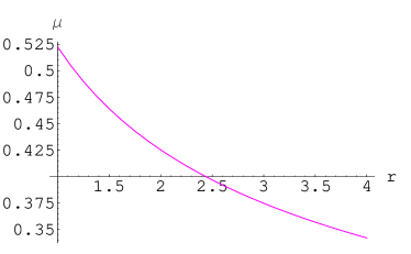
Figure 1: Both graphs have been plotted for $h_{1}=1$.

Figure 2: Both graphs have been plotted for $h_{1}=1$.

When $\alpha$ is $\frac{-5}{2}$ then $\Theta<0$ and matter density remains finite positive for the arbitrary choice of time profile. As $h_{1}=1$ and $\dot{h_{1}}=0$, so the contribution of electromagnetic field in this case vanish and density remains non-effective from electromagnetic field. The radial and transverse pressures are smoothly increasing and deceasing function of the electromagnetic field, respectively. As pressure increases in radial direction and decreases in transverse direction so anisotropy exists in the given system. The dimensionless anisotropy is smoothly increasing function of $s$. All these facts have been shown graphically in 1 and 2. The increase of anisotropy during gravitational collapse is due to the increasing strength of electromagnetic magnetic field. It is due to the fact that presence of electromagnetic field in any region of spacetime causes to disturb the generic behavior of the spacetime, so provide an external force which enhances the anisotropy.

3.2 Expansion with $\alpha=\frac{3}{2}$

For expansion, the rate of expansion must be positive, from Eq.(18), $\Theta>0$, when $\alpha>0$, also we assume that

$$R=(r^{2}+{r_{0}}^{2})^{-1}+h_{2}(t),$$ (36)

where $h_{2}(t)$ and $r_{0}$ are arbitrary function and constant, respectively. For $\alpha=\frac{3}{2}$ from Eqs.(19), (20) and (LABEL:19), we get

$$8\pi\mu = 4R-2{R^{-3}}\left[\frac{R^{\prime\prime}}{R}-\left(\frac{R^{\prime}}{R}\right)^{2}\right]+\frac{1}{R^{2}}-\frac{s^{2}{\dot{R}}^{2}}{R^{7}},$$ (37)

$$8\pi P_{r} = 4R+R^{-2}+2R^{-3}\left[\left(\frac{R^{\prime}}{R}\right)^{2}-\frac{\dot{R}^{\prime}}{\dot{R}}\frac{R^{\prime}}{R}\right]+\frac{s^{2}}{R},$$ (38)

$$8\pi P_{\perp} = -6R+{R^{-3}}\left[-\frac{1}{2}\frac{R^{\prime\prime}}{R}-\frac{7}{2}\frac{\dot{R}^{\prime}}{\dot{R}}\left(\frac{R^{\prime}}{R}\right)+\frac{\dot{R}^{\prime\prime}}{R}+3\left(\frac{R^{\prime}}{R}\right)^{2}\right]-\frac{s^{2}}{R^{4}}.$$

With $F(t,r)=1+h_{2}(t)(r^{2}+{r_{0}}^{2})$ and $R=\frac{F}{(r^{2}+{r_{0}}^{2})}$, the density and pressures in this case are

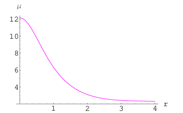
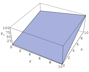
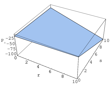
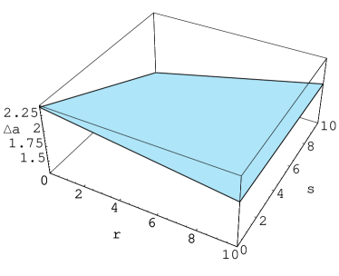
Figure 3: This graph is plotted for $h_{2}=1,r_{0}=1$.

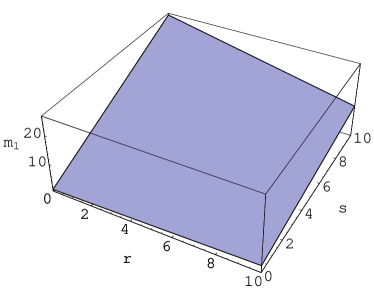
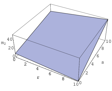
Figure 4: This graph is plotted for $h_{2}=1,r_{0}=1$.

Figure 5: This graph is plotted for $h_{2}=1,r_{0}=1$.

$$8\pi\mu = \frac{4F}{(r^{2}+{r_{0}}^{2})}+\frac{(r^{2}+{r_{0}}^{2})^{2}}{F^{2}}+\frac{4(r^{2}+{r_{0}}^{2})({r_{0}}^{2}-3r^{2})}{F^{4}}+\frac{8r^{2}(r^{2}+{r_{0}}^{2})}{F^{5}}$$ (40)

$$- \frac{s^{2}{\dot{h_{1}}}(r^{2}+{r_{0}}^{2})^{7}}{F^{7}},$$

$$8\pi P_{r} = \frac{4F}{(r^{2}+{r_{0}}^{2})}+\frac{(r^{2}+{r_{0}}^{2})^{2}}{F^{2}}+\frac{8r^{2}(r^{2}+{r_{0}}^{2})}{F^{5}}+\frac{s^{2}(r^{2}+{r_{0}}^{2})}{F},$$ (41)

$$8\pi P_{\perp} = \frac{-6F}{(r^{2}+{r_{0}}^{2})}+\frac{(r^{2}+{r_{0}}^{2})({r_{0}}^{2}-3r^{2})}{F^{4}}+\frac{12r^{2}(r^{2}+{r_{0}}^{2})}{F^{5}}-\frac{s^{2}(r^{2}+{r_{0}}^{2})^{4}}{F^{4}}.$$

The mass function Eq.(22), takes the following form

$$m_{2}(r,t)=\frac{F}{2(r^{2}+{r_{0}})}\left[\frac{s^{2}(r^{2}+{r_{0}})^{2}}{F^{2}}+1+\left(\frac{F^{3}}{2(r^{2}+{r_{0}})^{3}}-\frac{4r^{2}}{F^{3}(r^{2}+{r_{0}})}\right)\right].$$ (43)

The dimensionless measure of anisotropy defined by Eq.(4) in this case takes the following form

$$\triangle a=1+\frac{\frac{6F^{6}}{(r^{2}+{r_{0}}^{2})^{2}}-12r^{2}-F^{3}(r^{2}+{r_{0}}^{2})+F\left[r^{6}s^{2}-{r_{0}}^{2}+3r^{4}s^{2}{r_{0}}^{2}+3r^{2}(1+s^{2}{r_{0}}^{2})\right]}{\left(\frac{4F^{6}}{(r^{2}+{r_{0}}^{2})^{2}}+F^{4}s^{2}+8{r_{0}}^{2}+F^{3}(r^{2}+{r_{0}}^{2})\right)}.$$ (44)

As compared to gravitational collapse the reverse effects of electromagnetic field occur on pressures and anisotropy during the expansion. The expansion process causes to separate the charges apart from each other, this leads to weak the electromagnetic field intensity. Both the radial and transverse pressures are increasing functions while anisotropy decreases from maximum value to finite positive value. All these facts are shown in figures 3 and 4. The behavior of mass function in case of collapse and expansion is shown in right and left graphs of figure 5, respectively.

4 Conclusion

The general solution of anisotropic system has attained a considerable interest in Einstein theory of gravity due to their applications to stellar collapse of astrophysical objects. These solutions helps to discuss the anisotropy of the cosmological models. Barrow and Maartens (1998) have examined the effects of anisotropic pressures on the late-time behavior of inhomogeneous universe. They pointed that the decay of shear anisotropy can be determined by measurement of anisotropic stresses. According to Herrera and Santos (1997) in anisotropic highly dense system a phase transition would occur during the continual collapse of the gravitating source. They remarked that system may particularly transit to a pion condensed state. In this case a soften equation of state can provide a large amount of energy released during the collapse of massive source.

This paper deals with the study of generating solution of Einstein-Maxwell field equations with anisotropic spherically symmetric gravitating source. Misner-Sharp mass function with the contribution electromagnetic field as well as trapped surfaces have been studied in detailed. The condition ${R^{\prime}}=R^{2\alpha}$, implies the existence of two horizons at $R=m\pm\sqrt{m-s^{2}}$, provided $m\geq s$. This result is analogous to Reissner-Nordstrom solution if one replaces $s=Q$. This implies that the presence of electromagnetic field in the gravitating source is necessary and sufficient condition for the existence of more than one horizon. In this case $R_{+}$ and $R_{-}$ corresponds to outer and inner horizons, respectively. The curvature singularity is hidden at the common center of these horizons.

Under the condition ${R^{\prime}}=R^{2\alpha}$, the rate of expansion scalar becomes $\Theta=(2+\alpha)R^{(1-\alpha)}$. This implies that $\Theta=0$, for $\alpha=-2$, $\Theta>0$, for $\alpha>-2$, $\Theta<0$, for $\alpha<-2$, which corresponds to bouncing, expansion and collapse, respectively. For collapse the value of $\alpha$ is $\alpha=\frac{-5}{2}$ which implies that $\Theta<0$ and matter density is decreasing function of $r$ for the arbitrary choice of time profile. This becomes independent of electromagnetic field contribution for the given time profile. The radial and transverse pressures are increasing and deceasing function of the electromagnetic field contribution $s$. Since pressure increases in one direction while it increases in the other direction so the difference of pressures is non-zero which causes the anisotropy in the given system. The dimensionless anisotropy is increasing function of $s$. All these facts have been shown graphically in 1 and 2. The increase of anisotropy in this case is due to the increasing strength of electromagnetic magnetic field as charged come close to each other during gravitational collapse. It confers the fact that presence of electromagnetic field in any region of spacetime causes to disturb the generic behavior of the spacetime. So, increasing electromagnetic field during gravitational collapse causes to enhance the anisotropy.

On the other hand the reverse effects of electromagnetic field occur on pressure components and anisotropy during the expansion as electromagnetic field is weaker in this case as compared to collapsing case. The expansion process causes to separate the charges apart from each other this leads to weak the electromagnetic field. Both the radial and transverse pressures are increasing functions while anisotropy decreases from maximum value to finite positive value. All these facts are shown in figures 3 and 4. The Electromagnetic field decreases the collapse and increases the expansion as well as bouncing by producing the repulsive in the system.

Acknowledgment

We highly appreciate the fruitful comments of the anonymous referee for the improvements of the paper.

References

- [1] Ardavan, H., Partovi, M.H.: Phys. Rev. D16(1977)1664
- [2] Abbas, G.: Astrophys. Space Sci. 350(2014a)307
- [3] Abbas, G.: Sci. China. Phys. Mech. Astro 57(2014b)604
- [4] Abbas, G.: Adv. High Energy Phys. 2014(2014c)306256
- [5] Bayin, S.S.: Phys. Rev. D26(1982)1262
- [6] Bondi, H.: MNRAS 259(1992)365
- [7] Barcelo, C., Liberati, S., Sonego, S., Visser, M.: Phys. Rev. D77(2008)044032
- [8] Barrow, J.D., Maartens, R. G.: Phys. Rev. D59(1998)043502
- [9] Cosenza, M., Herrera, L., Esculpi, M., Witten, L.: J. Math. Phys. A 22(1981)118
- [10] Cognola, G., Elizalde, E., Nojiri, S, Odintov, S.D., Zerbini, S.: Phys. Rev. D75(2007)086002
- [11] Di Prisco, A., Herrera, L., Denmat, G.Le., MacCallum, M.A.H., Santos, N.O.: Phys. Rev. D76(2007)064017
- [12] Darmois, G.: Memorial des Sciences Mathematiques (Gautheir-Villars, Paris, (1927) Glass, E.N.: Phys. Lett. A86(1981)351
- [13] Glass, E.N.: Gen. Relativ. Gravit. 45(2013)2661
- [14] Gasperini, M., Veneziano, G.: Astropart. Phys. 1(1993)317
- [15] Germani, C., Tsagas, C.G.: Phys. Rev. D73(2006)064010
- [16] Herrera, L., Di Prisco, A., Ibanez, J.: Phys. Rev. D84(2011)107501
- [17] Herrera, L., Ospino, J., Di Prisco, A.: Phys. Rev. D77, (2008)027502
- [18] Herrera, L., Santos, N.O., Wang, A.: Phys. Rev. D78(2008)084024
- [19] Hawking, S.W., Ellis, G.F.R.: The Large Scale Structure of Spacetime (Cambridge University Press, 1979)
- [20] Herrera, L., Santos, N.O.: Phys. Rep. 286(1997)53
- [21] Joshi, P.S.: Global Aspects in Gravitation and Cosmology (Oxford University Press, (1993)
- [22] Misner, C.W., Sharp, D.: Phys. Rev. 136(1964) B571
- [23] Misner C.W. and Sharp, D.H.: Phys. Lett. 15(1965)279
- [24] Nojiri, S., Odintov, S.D.: Phys. Lett. B631(2005)1
- [25] Nojiri, S., Odintov S.D., Gorbunova, O.G.: J. Phys. A39(2006)6627
- [26] Oppenheimer, J.R., Snyder, H.: Phys. Rev. 56(1939)455
- [27] Penrose, R.: Riv. Nuovo Cimento 1(1969)252
- [28] Sharif, M., Abbas, G.: J. Phys. Soc. Jpn. 82, (2013a)034006
- [29] Sharif, M., Abbas, G.: Chinese Phys. B22, (2013b)030401
- [30] Sharif, M., Abbas, G.: Eur. Phys. J. Plus 28, (2013c)10
- [31] Stein-Schabes, J.A.: Phys. Rev. D31(1985)1838
- [32] Sharif, M., Bhatti, M.Z.: Gen. Relativ. Gravit. 44(2012a)281
- [33] Sharif, M., Bhatti, M.Z.: Mod. Phys. Lett. A27(2012b)1250141
- [34] Sharif, M., Yousaf, Z.: Can. J. Phys. 90, 865(2012)
- [35] Thorne, K.S.: Phys. Rev. 138(1965)B251
- [36]