Experimental generation of an optical field with arbitrary spatial coherence properties

Abstract

We describe an experimental technique to generate a quasi-monochromatic field with any arbitrary spatial coherence properties that can be described by the cross-spectral density function, $W(\mathbf{r_{1}},\mathbf{r_{2}})$. This is done by using a dynamic binary amplitude grating generated by a digital micromirror device (DMD) to rapidly alternate between a set of coherent fields, creating an incoherent mix of modes that represent the coherent mode decomposition of the desired $W(\mathbf{r_{1}},\mathbf{r_{2}})$. This method was then demonstrated experimentally by interfering two plane waves and then spatially varying the coherence between them. It is then shown that this creates an interference pattern between the two beams whose fringe visibility varies spatially in an arbitrary and prescribed way.

I Introduction

The transverse degree of freedom of an optical field is the fundamental aspect of light that contains spatial information. Utilization of this information is the basic resource in traditional imaging systems and in applications such as microscopy, lithography, holography or metrology. In addition, use of the transverse modes of light has recently been demonstrated to be an important resource in optical communication Wang2012 ; Rodenburg2012 ; Mirhosseini2013 ; Boyd2011 , high-dimensional entanglement studies Mair2001a ; Dada2011 , and Quantum key distribution Boyd2011a ; Malik2012 .

Having control of the spatial coherence properties of a light beam provides an additional degree of control compared to using fully coherent light only, and has been shown to be advantageous for a number of applications. Beams of decreased coherence allow access to spatial frequencies that are twice those available in a purely coherent system Considine1966 . Greater spatial frequencies can enable improvements in imaging based systems and has been shown to be particularly useful in lithography Lin1980 . Partial coherence also allows for the suppression of unwanted coherent effects by decreasing the coherence, such as suppression of speckle Dainty1970 which enables lower noise and opens the door to novel imaging modalities Dubois1999 . It has also been suggested that partial coherence can improve the deleterious effects of optical propagation through random or turbulent media Gbur2002 . In addition, the coherent property of optical beams can be used for novel beam shaping Lajunen2011 as well as a method for control over soliton formation due to modulation instabilities in the study of nonlinear beam dynamics Chen2002 . The ability to generate arbitrary optical beams could also be used as a tool in basic research, such as in optical propagation Waller2012 or testing of novel methods in quantum state tomography dealing with the transverse wavefunction of light that has seen a great deal of interest recently Lundeen2011 ; Lundeen2012 . Traditional methods used to generate partially coherent beams of light often rely on imprinting a changing pattern of random phase or speckle onto a coherent beam, such as with a spatial light modulator (SLM) Rickenstorff2012 or rotating diffuser Baleine2004 . It has even been demonstrated that SLMs allow the statistics of the speckle patterns to be varied across the beam to give spatially varying coherence properties Waller2012 . However none of these methods have been shown to allow for complete arbitrary control over the spatial coherence of an optical beam.

In this paper we demonstrate how to generate any arbitrary quasi-monochromatic partially coherent field that can be specified by a cross-spectral density function $W(\mathbf{r_{1},r_{2}})$, i.e. for fields fully specified by their two point spatial correlations. This is done by first computing the coherent mode decomposition of $W(\mathbf{r_{1},r_{2}})$, which is an incoherent mixture of orthogonal coherent modes. For each of these coherent modes a computer generated hologram (CGH) is computed for a digital micromirror device (DMD) that acts as a binary amplitude spatial light modulator with rapid modulation speeds. The DMD then switches between each coherent mode on timescales slower than the coherence time of the source laser, but long relative to the detection time of the CCD. This creates an incoherent averaging that physically reproduces the coherent mode decomposition. Section II details computation of the coherent mode decomposition, section III describes the algorithm to compute binary amplitude CGHs for the generation of coherent modes and section IV details the experimental demonstration of this technique.

II Coherent mode decomposition

The transverse wavefront of a deterministic and coherent scalar beam is described by a complex field, $U(\mathbf{r})$. For a stochastic beam, $U(\mathbf{r})$ is a random variable and it becomes necessary to represent the field in a more sophisticated way. The standard way of doing this is with the cross-spectral density function. At a single frequency the cross-spectral density function is defined as

$$W(\mathbf{r_{1}},\mathbf{r_{2}})=\left<U^{*}(\mathbf{r_{1}})U(\mathbf{r_{2}})\right>,$$ (1)

and represents the average intensity ($\Braket{I(r)}\equiv W(\mathbf{r,r})$), as well as the correlations (up to second order) of such a partially coherent field Mandel1995 .

$W(\mathbf{r_{1}},\mathbf{r_{2}})$ can be decomposed into an incoherent sum of orthogonal spatial modes $\psi_{n}(\mathbf{r})$, written as

$$W(\mathbf{r_{1}},\mathbf{r_{2}})=\sum_{n}{\lambda_{n}\psi_{n}^{*}(\mathbf{r_{1}})\psi_{n}(\mathbf{r_{2}})},$$ (2)

where $\lambda_{n}$ are real and nonnegative, and $p_{n}=\lambda_{n}/\sum\lambda_{n}$ is the relative weight of the field in mode $\psi_{n}(\mathbf{r})$ Wolf1981 . The modes $\psi_{n}(\mathbf{r})$ can be computed as the eigenfunctions with corresponding eigenvalues $\lambda_{n}$ from the Fredholm integral equation

$$\int{W(\mathbf{r_{1}},\mathbf{r_{2}})\psi_{n}(\mathbf{r_{1}})\,\mathrm{d}^{2}\mathbf{r_{1}}}=\lambda_{n}\psi_{n}(\mathbf{r_{2}}).$$ (3)

This representation is often referred to as a coherent mode decomposition of $W(\mathbf{r_{1}},\mathbf{r_{2}})$. Mathematically Eq. 2 is a sum over an infinite number of modes, but in practice $n$ is bounded by the maximum spatial frequency content of $W(\mathbf{r_{1},r_{2}})$, i.e. there is some maximum $n_{max}=N$ such that for $n>N$, $p_{n}$ will be negligibly small. For example, Gaussian Schell-model beams are a common example of a partially coherent beam. Such a beam is defined by having a Gaussian intensity $I(\mathbf{r})=\exp{(-r^{2}/2\sigma_{I}^{2})}$, as well as a Gaussian degree of coherence $\mu(\mathbf{r_{1},r_{2}})=\exp{(-|\mathbf{r_{1}-r_{2}}|^{2}/2\sigma_{\mu}^{2})}$, which gives a cross-spectral density function

$$W(\mathbf{r_{1},r_{2}})=\sqrt{I(\mathbf{r_{1}})I(\mathbf{r_{2}})}\mu(\mathbf{r_{1},r_{2}}).$$ (4)

A coherent mode decomposition of such a Gaussian Schell-model beam shows that the number of coherent modes necessary to describe Eq. 4 is given by the number of independent coherent regions within the beam which is quantified by $N\approx(\sigma_{\mu}/\sigma_{I})^{2}$ Starikov1982 .

Physically Eq. 2 can be realized if one can create a beam that alternates between the coherent modes $\psi_{n}(\mathbf{r})$ in time with relative frequency weighted by $p_{n}$. For measurement to yield the intended field, the switching time $\tau_{s}$ must be much faster than any detector integration time $\tau_{det}$ in order to create the intended averaging over the inputs. In addition, for the mixture to be an incoherent mixture, the various modes must not have any correlations in time. Thus the switching time must be slower than the coherence time $\tau_{coh}$ of the source. Together these form the condition

$$\tau_{det}>\tau_{s}>\tau_{coh}.$$ (5)

If Eq. 5 is met, then one has a physically realized implementation of $W(\mathbf{r_{1},r_{2}})$.

III Generating Arbitrary Coherent Fields with Binary Gratings

In order to generate an arbitrary partially coherent field $W(\mathbf{r_{1},r_{2}})$, one only needs to find a way to create the coherent fields $\psi_{n}(\mathbf{r})$ in rapid succession. Such rapid mode generation was recently demonstrated by using DMDs to create quickly addressable binary amplitude modulated CGHs Mirhosseini2013a , though this comes at the cost of having a maximum efficiency around 10%. DMDs are devices that provide both the speed and resolution desired for rapid generation and switching of coherent fields Dudley2003 . A DMD consists of a 2-dimensional array of mirrors that can be in one of two positions, which can be used to act as an on or off state at each pixel. Each pixel can be individually addressed and changed very rapidly, at frame rates exceeding $10\,\mathrm{kHz}$.

Figure 1: Left: A binary amplitude grating composed of a series of rectangular pulses diffracting light into multiple orders. Middle: Pulse position modulation where a phase change is induced in the diffracted order as a result of a shift in the pulses. Right: Change in the amplitude of the diffracted order by pulse width modulation in which the diffraction efficiency is varied by changing the duty cycle of the binary pulses.

The fact that DMDs have 2 settings, allows us to make a binary grating. Any periodic structure acts as a diffraction grating. A transverse shift in this diffraction grating will induce a phase shift or detour phase in the diffracted orders, even if the grating is an amplitude only structure. In addition, the form of each period will determine the scattering efficiency into the diffracted order. Taken together, modulating the grating position and each periodic form locally within the hologram allows one to control both the amplitude and phase, and thus create any field, $U(\mathbf{r})=A(\mathbf{r})\exp{\left(i\phi(\mathbf{r})\right)}$ in the diffracted order.

A well known method of encoding binary holograms is to create a periodic array of binary fringes or rectangular ‘pulses.’ A one dimensional representation of this is shown in Fig. 1. A shift in the location of these pulses will change the overall phases into the diffracted orders, while changing the widths or duty cycles of the pulses will change the diffracted efficiency. These two methods are known as pulse position and pulse width modulation respectively Brown1969 ; Lee1979 ; Mirhosseini2013a , and such a modulation represents a generalization of the Moiré technique Zhang2011 . Mathematically, a periodic binary grating can be written as a Fourier series

$$f(\mathbf{r})=\sum_{m}\frac{\sin{(\pi mq)}}{\pi m}e^{im(\mathbf{G\cdot r}+2\pi\delta)},$$ (6)

where $\mathbf{G}=\frac{2\pi}{T}(\cos(\theta)\mathbf{\hat{x}}+\sin(\theta)\mathbf{\hat{y}})$ is the grating wavevector. The grating consists of rectangular pulses of width $qT$ spaced at a period of $T$ and $\delta\in[-1/2,1/2]$ is the relative location of the array within each period. Looking only at the first diffraction order $m=1$ the field is given by

$$U_{1}=U_{in}*\frac{\sin{(\pi q)}}{\pi}e^{i2\pi\delta},$$ (7)

where $U_{in}$ is the input field, which we’ll assume to be a constant plane wave. In addition all optics after the DMD are aligned along the axis of the first diffraction order, allowing us to ignore any phase tilt from $U_{in}$ as well as the $e^{i\mathbf{G\cdot r}}$ tilt from the grating in our description of $U_{1}$.

We can allow $q$ and $\delta$ to become functions of position and the previous results still hold so long as $q(\mathbf{r})$ and $\delta(\mathbf{r})$ vary much slower than the grating period $T$. Then any complex field $A(\mathbf{r})e^{i\phi(\mathbf{r})}$ can be generated by allowing

$$q(\mathbf{r})=\frac{1}{\pi}\arcsin{\left(A(\mathbf{r})\right)},\qquad\delta(\mathbf{r})=\frac{\phi{(\mathbf{r})}}{2\pi},$$ (8)

where the phase is $\phi\in[-\pi,\pi],$ which is defined symmetrically around 0 to avoid encoding errors in the presence of a varying amplitude Bolduc2013 .

This full procedure can be represented in the following fashion. First one chooses the field $U=A(\mathbf{r})e^{i\phi(\mathbf{r})}$ that one wishes to create. Then $q(\mathbf{r})$ and $\delta(\mathbf{r})$ are computed from Eq. 8 and a periodic sinusoidal function is computed to give

$$\cos\left(\mathbf{G\cdot r}+2\pi\delta(\mathbf{r})\right).$$ (9)

To convert this into a binary hologram, this function is thresholded by $\cos(\pi q(\mathbf{r}))$ to create a binary pulse train with local pulse width $q(\mathbf{r})$. This can be written in the compact form

$$f(\mathbf{r})=\operatorname{H}\left[\cos\left(\mathbf{G\cdot r}+2\pi\delta(\mathbf{r})\right)-\cos(\pi q(\mathbf{r}))\right],$$ (10)

where $\operatorname{H}(z)$ is the Heaviside step function defined as

$$\operatorname{H}(z)\equiv\begin{cases}0&\quad\text{if $z<0$}\\ 1&\quad\text{if $z\geq 0$}\end{cases}.$$ (11)

IV Experiment

A schematic of the experimental setup is shown in Fig. 2. A HeNe laser is spatially filtered using a 4f system to provide an initial coherent plane wave incident on the DMD. The various coherent modes, $\psi_{n}$, are created in rapid succession with a spatially modulated binary diffraction grating on the DMD that gives the desired field in the first diffraction order. A second 4f system and pinhole are used to filter out all other diffraction orders and the resultant beam is imaged onto a CCD camera.

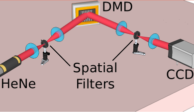
Figure 2: Experimental setup used to generate any field, $W(\mathbf{r_{1}}\mathbf{r_{2}})$. A fully spatially coherent plane wave is prepared by spatial filtering of a HeNe laser. This collimated beam is reflected off a CGH generated by the DMD and the desired diffracted order is filtered by a 4f system and imaged onto a CCD.

The DMD is a type of micro-electronic mechanical system, commonly known as a MEMS, that can function as an amplitude only SLM Dudley2003 . The device consists of a two dimensional pixelated array of micromirrors each mounted on an individually addressed MEMS that can be in one of two positions. In order to use the device as a SLM, the device is aligned such that the light is reflected and collected by the optics after the DMD if the micromirrors are in the on position, but scattered out of the system if the mirrors are in the off position. The device used in the experiment was a Texas Instrument DLP3000. This device has a display resolution of $608\times 684$ pixels, a micromirror size of $7.5\,\mathrm{\mu m}$, and the pixels can be switched at rates up to 4 KHz which is much faster than a typical phase based SLM Mirhosseini2013a .

The CCD operates at 60 Hz, thus the detector integration time is $\tau_{det}=1/60\,\mathrm{Hz}\approx 17\,\mathrm{ms}$. The DLP3000 DMD used in this experiment has a switching rate of 4 kHz, thus $\tau_{s}=1/4\,\mathrm{kHz}=250\,\mathrm{\mu s}<\tau_{det}$, which fulfills the first inequality in Eq. 5. The bandwidth of the HeNe is 1.5 GHz which gives $\tau_{coh}=1/1.5\,\mathrm{GHz}\approx 0.7\,\mathrm{ns}$ which meets the second part of the inequality in Eq. 5.

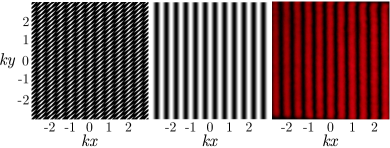
Figure 3: Interference fringes formed from the coherent superposition of two plane waves. Left figure shows the CGH used to generate the desired mode. Middle figure represents the target image while the right figure is an experimental image of the generated mode.

As a demonstration of the ability to generate a single coherent state the field

$$U(\mathbf{r})\propto e^{ikx}+e^{-ikx}$$ (12)

was generated. This represents a coherent superposition of two plane wave states, which form a sinusoidal interference pattern as shown in Fig 3.

For this experiment the mode was generated using a grating with wavevector

$$\mathbf{G}=\frac{2\pi}{25\,\mathrm{px}}(\mathbf{\hat{x}}+\mathbf{\hat{y}}),$$ (13)

which represents a period of $T=25\sqrt{2}\,\mathrm{pixels}\approx 275\,\mathrm{\mu m}$ oriented at $\theta=45^{\circ}$. This value of $\mathbf{G}$ was chosen to be large enough to allow enough separation in the Fourier plane to allow for filtering of the 1st diffracted order with an iris. In addition a nonzero value was chosen for both the $x$ and $y$ components of $\mathbf{G}$ in order to minimize the noise by ensuring that the diffracted order did not overlap with any specular reflection due to the DMD’s imperfect pixel fill-fraction. The underlying grating can be seen in the left image in Fig. 3 which have the appearance of the small diagonally oriented slivers. The plane wave transverse wavenumber was chosen to be

$$k=\frac{2\pi}{100\,\mathrm{px}}\approx\frac{2\pi}{780\,\mathrm{\mu m}}.$$ (14)

$k\ll|\mathbf{G}|$ and thus is slowly varying enough to allow us to use the procedure in section III to construct the CGH to create this state. Since we are perfectly interfering 2 plane waves, the intensity varies as $I\propto\cos^{2}(kx)$. Therefore $q(\mathbf{r})=\arcsin(\cos(kx))/\pi$, while $\delta(\mathbf{r})=0$.

Next we created a superposition of the plane waves $U_{A}=e^{ikx}$ and $U_{B}=e^{-ikx}$ as before, but this time the degree of coherence between the two beams was spatially varied, creating a partially coherent mix of modes. The coherent modes used to represent this is given by

$$\begin{split}\psi_{1}(\mathbf{r})&\propto(U_{A}+f(\mathbf{r})U_{B})\\ \psi_{2}(\mathbf{r})&\propto(f(\mathbf{r})U_{A}+U_{B}),\end{split}$$ (15)

where the relative probability weightings are given as $p_{1}=p_{2}=1/2$, and where $f(\mathbf{r})$ is related to the fringe visibility $V(\mathbf{r})$ by

$$f(\mathbf{r})=V(\mathbf{r})/(1+\sqrt{1-V(\mathbf{r})^{2}}).$$ (16)

The intensity for this beam is

$$I(\mathbf{r})\propto(1-f)^{2}+4f\cos^{2}(kx),$$ (17)

which is the sum of an incoherent and a coherent term which can be continuously tuned from fully coherent ($f=1$) to incoherent ($f=0$).

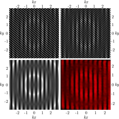
Figure 4: Interference fringes formed from superposition of two plane waves that are partially coherent with respect to each other. Top figures show the CGHs used to generate the desired modes given by Eq. 16. Bottom left figure represents the target intensity pattern, while the bottom right figure is an experimental image of the generated field.

The visibility function chosen for the experiment is given by

$$V(\mathbf{r})=|\sin(\kappa r)|,$$ (18)

where

$$2\pi\kappa=\frac{4k}{3}=\frac{2\pi}{75\,\mathrm{px}}\approx\frac{2\pi}{580\,\mathrm{\mu m}}.$$ (19)

Since $f(\mathbf{r})$ was chosen to be real, Eq. 18 also represents our spectral degree of coherence at $\mathbf{r}$. The CGHs necessary to create the modes $\psi_{1}$ and $\psi_{2}$ (Eq. 15) for this spatially varying fringe visibility are shown in the top row of Fig. 4. The CGH parameters are

$$q(\mathbf{r})=\frac{1}{\pi}\arcsin\left(\frac{\sqrt{4f\cos^{2}(kx)+(1-f)^{2}}}{I_{\text{max}}}\right),$$ (20)

where $I_{\text{max}}$ is the maximum value of $I(\mathbf{r})$ and

$$\begin{split}\delta_{1,2}(\mathbf{r})&=\arg(\Re(\psi_{1,2})+i\Im(\psi_{1,2}))\\ &=\arg((2\cos(kx)-(1-f)\cos(kx))\\ &\qquad\mp i((f-1)\sin(kx))).\end{split}$$ (21)

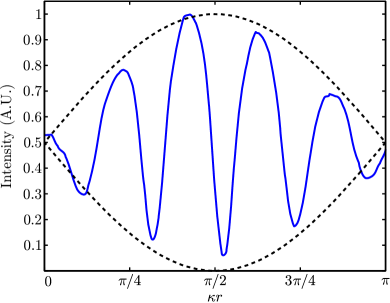
Figure 5: Plot of the intensity of the image in Fig. 4 along the 1D slice of $r$ for $\theta=0$, i.e. along the $x$-axis (solid blue line). Also shown as the black dotted line is the theoretical envelope of the maximum and minimum intensities based on the intended visibility function $V(\mathbf{r})$.

In order to compare the intended visibility given by Eq. 18 with the image shown in Fig. 4, a one dimensional slice of the intensity is plotted in Fig. 5. This slice is a radial slice $r$ along the $x$ axis (i.e. at an orientation of $\theta=0$), and is plotted over an entire period of $\sin(\kappa r)$ of the visibility. In addition the theoretical envelope of the visibility equal to $(1\pm V(\mathbf{r}))/2=(1\pm|\sin(\kappa r)|)/2$ is plotted for comparison. As can be seen in both the original coherent and partially coherent cases, the intended and measured patterns are in excellent agreement with one another.

V Conclusions

In this paper we have demonstrated a novel method of generating arbitrary fields of light. Any partially coherent field that is described by the cross-spectral density function $W(\mathbf{r_{1},r_{2}})$ can be generated by computing the coherent mode decomposition into an incoherent sum of coherent modes. This incoherent mix of modes was physically realized by rapid generation of spatial holograms on a DMD and was temporally averaged in detection.

We acknowledge Mayukh Lahiri, Joe Vornehm and Alex Radunsky for helpful discussions. Our work was supported by the Defense Advanced Research Projects Agency (DARPA) InPho program and OSML also acknowledges support from the CONACyT.

References

- (1) J. Wang, J.-Y. Yang, I. M. Fazal, N. Ahmed, Y. Yan, H. Huang, Y. Ren, Y. Yue, S. Dolinar, M. Tur, and A. E. Wilner, “Terabit free-space data transmission employing orbital angular momentum multiplexing,” Nature Photonics 6, 488–496 (2012).
- (2) B. Rodenburg, M. P. J. Lavery, M. Malik, M. N. O’Sullivan, M. Mirhosseini, D. J. Robertson, M. J. Padgett, and R. W. Boyd, “Influence of atmospheric turbulence on states of light carrying orbital angular momentum,” Opt. Lett. 37, 3735 (2012).
- (3) M. Mirhosseini, B. Rodenburg, M. Malik, and R. W. Boyd, “Free-space communication through turbulence: a comparison of plane-wave and orbital-angular-momentum encodings,” J. Mod. Opt. 61, 43–48 (2014).
- (4) R. W. Boyd, B. Rodenburg, M. Mirhosseini, and S. M. Barnett, “Influence of atmospheric turbulence on the propagation of quantum states of light using plane-wave encoding,” \opex19, 18310 (2011).
- (5) A. Mair, A. Vaziri, G. Weihs, and A. Zeilinger, “Entanglement of the orbital angular momentum states of photons.” Nature 412, 313–6 (2001).
- (6) A. C. Dada, J. Leach, G. S. Buller, M. J. Padgett, and E. Andersson, “Experimental high-dimensional two-photon entanglement and violations of generalized Bell inequalities,” Nature Physics 7, 677–680 (2011).
- (7) R. W. Boyd, A. Jha, M. Malik, C. O’Sullivan, B. Rodenburg, and D. J. Gauthier, “Quantum key distribution in a high-dimensional state space: exploiting the transverse degree of freedom of the photon,” Proceedings of SPIE 7948, 79480L–6 (2011).
- (8) M. Malik, M. N. O’Sullivan, B. Rodenburg, M. Mirhosseini, J. Leach, M. P. J. Lavery, M. J. Padgett, and R. W. Boyd, “Influence of atmospheric turbulence on optical communications using orbital angular momentum for encoding,” \opex20, 13195 (2012).
- (9) P. S. Considine, “Effects of Coherence on Imaging Systems,” Journal of the Optical Society of America 56, 1001 (1966).
- (10) B. Lin, “Partially coherent imaging in two dimensions and the theoretical limits of projection printing in microfabrication,” IEEE Transactions on Electron Devices 27, 931–938 (1980).
- (11) J. Dainty, “Some Statistical Properties of Random Speckle Patterns in Coherent and Partially Coherent Illumination,” Optica Acta: International Journal of Optics 17, 761–772 (1970).
- (12) F. Dubois, L. Joannes, and J.-C. Legros, “Improved Three-Dimensional Imaging with a Digital Holography Microscope With a Source of Partial Spatial Coherence,” Appl. Opt. 38, 7085 (1999).
- (13) G. Gbur and E. Wolf, “Spreading of partially coherent beams in random media,” J. Opt. Soc. Am. A 19, 1592 (2002).
- (14) H. Lajunen and T. Saastamoinen, “Propagation characteristics of partially coherent beams with spatially varying correlations,” Optics Letters 36, 4104–4106 (2011).
- (15) Z. Chen, S. M. Sears, H. Martin, D. N. Christodoulides, and M. Segev, “Clustering of solitons in weakly correlated wavefronts,” Proceedings of the National Academy of Sciences 99, 5223–5227 (2002).
- (16) L. Waller, G. Situ, and J. W. Fleischer, “Phase-space measurement and coherence synthesis of optical beams,” Nature Photonics 6, 474–479 (2012).
- (17) J. S. Lundeen, B. Sutherland, A. Patel, C. Stewart, and C. Bamber, “Direct measurement of the quantum wavefunction.” Nature 474, 188–91 (2011).
- (18) J. S. Lundeen and C. Bamber, “Procedure for Direct Measurement of General Quantum States Using Weak Measurement,” Phys. Rev. Lett. 108, 070402 (2012).
- (19) C. Rickenstorff, E. Flores, M. Olvera-Santamaría, and A. Ostrovsky, “Modulation of coherence and polarization using nematic 90 degree-twist liquid-crystal spatial light modulators,” Revista mexicana de física 58, 270–273 (2012).
- (20) E. Baleine and A. Dogariu, “Variable-coherence tomography for inverse scattering problems,” J. Opt. Soc. Am. A 21, 1917 (2004).
- (21) L. Mandel and E. Wolf, Optical Coherence and Quantum Optics (Cambridge University Press, 1995).
- (22) E. Wolf, “New spectral representation of random sources and of the partially coherent fields that they generate,” Opt. Commun. 38, 3–6 (1981).
- (23) A. Starikov and E. Wolf, “Coherent-mode representation of Gaussian Schell-model sources and of their radiation fields,” Journal of the Optical Society of America 72, 923 (1982).
- (24) M. Mirhosseini, O. S. Magaña Loaiza, C. Chen, B. Rodenburg, M. Malik, and R. W. Boyd, “Rapid generation of light beams carrying orbital angular momentum,” \opex21, 30196 (2013).
- (25) D. Dudley, W. M. Duncan, and J. Slaughter, “Emerging digital micromirror device (DMD) applications,” Proc. SPIE 4985, 14–25 (2003).
- (26) B. R. Brown and A. W. Lohmann, “Computer-generated Binary Holograms,” IBM Journal of Research and Development 13, 160–168 (1969).
- (27) W.-H. Lee, “High efficiency multiple beam gratings,” Appl. Opt. 18, 2152 (1979).
- (28) P. Zhang, Z. Zhang, J. Prakash, S. Huang, D. Hernandez, M. Salazar, D. N. Christodoulides, and Z. Chen, “Trapping and transporting aerosols with a single optical bottle beam generated by moiré techniques.” Optics letters 36, 1491–3 (2011).
- (29) E. Bolduc, N. Bent, E. Santamato, E. Karimi, and R. W. Boyd, “Exact solution to simultaneous intensity and phase encryption with a single phase-only hologram,” Opt. Lett. 38, 3546–3549 (2013).