Recent work has demonstrated that the infrared effects of harmonic oscillator basis truncations are well approximated by a partial-wave Dirichlet boundary condition at a properly identified radius $L$. This led to formulas for extrapolating the corresponding energy $E_{L}$ and other observables to infinite $L$ and thus infinite basis size. Here we reconsider the energy for a two-body system with a Dirichlet boundary condition at $L$ to identify and test a consistent and systematic expansion for $E_{L}$ that depends only on observables. We also generalize the energy extrapolation formula to nonzero angular momentum, and apply it to the deuteron. Formulas given previously for extrapolating the radius are derived in detail.

Systematic expansion for infrared oscillator basis extrapolations

I Introduction

The use of finite harmonic oscillator (HO) model spaces in nuclear structure calculations effectively imposes both infrared (IR) and ultraviolet (UV) momentum cutoffs Stetcu et al. (2007); Hagen et al. (2010); Jurgenson et al. (2011); Coon et al. (2012); Furnstahl et al. (2012). Computational limits often require that the HO basis be truncated before observables are fully converged, which has led to various phenomenological schemes to extrapolate energies to infinite basis size Hagen et al. (2007); Bogner et al. (2008); Forssen et al. (2008); Maris et al. (2009); Roth (2009). More systematic development of extrapolation formulas is possible by considering the IR and UV cutoffs explicitly, as first illustrated in Ref. Coon et al. (2012). A theoretical basis for the IR extrapolation was proposed in Ref. Furnstahl et al. (2012) (together with a model for combined IR and UV extrapolations), and further developed in Ref. More et al. (2013).

These papers demonstrate that oscillator basis truncations (and more general basis truncations) effectively impose a Dirichlet boundary condition (bc) at a properly identified radius $L$ in position space. The radius $L$ is related to the smallest eigenvalue $\kappa^{2}$ of the squared momentum operator $\hat{p}^{2}$ in the finite basis, and $\kappa=\pi/L$. For the oscillator basis with highest excitation energy $N\hbar\Omega$, a very accurate approximation is More et al. (2013)

$$L=L_{2}\equiv\sqrt{2(N+3/2+2)}b\;,$$ (1)

where $b=\sqrt{\hbar/(\mu\Omega)}$ is the oscillator length for a particle with (reduced) mass $\mu$ and an oscillator frequency $\Omega$. The maximum excitation energy of the single-particle basis is $N=2n+l$ in terms of the radial quantum number $n$ and the angular momentum $l$. Note that $L_{2}$ differs slightly from the naive estimate $L_{0}=\sqrt{2(N+3/2)}b$. In localized bases that differ from the harmonic oscillator, $L$ can be determined from a numerical diagonalization of the operator $\hat{p}^{2}$.

The diagonalization of $\hat{p}^{2}$ shows that its low-lying spectrum in a finite oscillator basis resembles that of a particle in a spherical cavity of radius $L_{2}$ More et al. (2013). Therefore, the use of a Dirichlet boundary condition at $L_{2}$ is a very convenient way to understand the long-wavelength consequences of a finite basis. The difference between a Dirichlet bc and the real asymptotic behavior of oscillator wave functions are high-momentum modes, as can be shown by considering Fourier transforms of the low-lying eigenstates (an example is given in Fig. 1). Thus, this difference is irrelevant for long-wavelength physics of bound states. We note that the use of a Dirichlet bc is similar in spirit to the use of contact interactions to describe the effect of unknown short-ranged forces on long-wavelength probes.

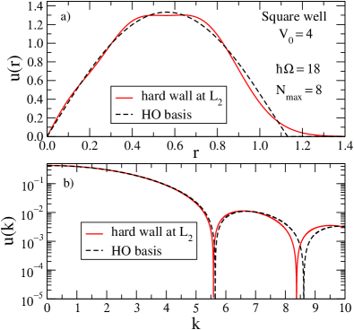
Figure 1: (color online) Ground-state wave functions for a square well potential of depth $V_{0}=4$ (see Eq. (19); lengths are in units of $R$ and energies in units of $1/R^{2}$ with $\hbar^{2}/\mu=1$) from solving the Schrödinger equation with a truncated harmonic oscillator basis with $\hbar\Omega=18$ and $N=8$ (dashed) and with a Dirichlet boundary condition at $r=L_{2}$ given from Eq. (1) (solid). The coordinate-space radial wave functions in a) exhibit a difference at $r$ near 1.5, but the Fourier-transformed wave functions in b) are in close agreement at low $k$, showing that the differences are high-momentum modes.

A Dirichlet bc at $r=L$ allows one to derive formulas to extrapolate bound-state energies and radii to infinite basis, and to predict scattering phase shifts from the finite model space results More et al. (2013). In a simple view, the Dirichlet bc introduces too much curvature into a bound-state wave function, and the corresponding change in kinetic energy can be derived accordingly. For applications and tests of the extrapolations formulas we refer the reader to Refs. Soma et al. (2013); Hergert et al. (2013); Jurgenson et al. (2013); Sääf and Forssén (2014); Roth et al. (2013).

We note that the IR extrapolation formulas Furnstahl et al. (2012) attain for the oscillator basis (or any localized finite basis) what Lüscher’s formula Lüscher (1986) achieves for the lattice. The Lüscher method has been extended to two-body bound states with many recent developments (e.g., see Refs. Lee and Pine (2011); Davoudi and Savage (2011); Koenig et al. (2011); Pine and Lee (2013); Briceño et al. (2013)). Here, the oscillator basis has the advantage that two-body bound-state extrapolations (e.g., see Ref. More et al. (2013)) are technically not more complicated than for one-body systems. In a discrete variable representation, IR and UV errors can also be accessed conveniently Bulgac and Forbes (2013).

The extrapolation formulas of Refs. Furnstahl et al. (2012) and More et al. (2013) were derived in a model-independent way based on the so-called linear energy method Djajaputra and Cooper (2000). In the present work we reconsider the problem of a two-body system with Dirichlet bc at $L$ to construct a consistent and systematic expansion for the bound-state energy $E_{L}$ using a more general method based on expanding the S-matrix about the bound-state pole in complex momentum. This approach can be directly applied beyond $s$-waves and to coupled channels, and manifests that $E_{L}$ depends only on observables. We extend the results in More et al. (2013) to next-to-leading order (NLO), correcting an inconsistent higher-order formula, and demonstrate well-defined theoretical uncertainties for model problems and a realistic deuteron calculation that uses a truncated oscillator basis (with a range of oscillator parameters chosen so that the UV contamination is negligible).

The plan of the paper is as follows. In Sec. II we use an analytic continuation of the S-matrix to complex momentum to derive a transcendental equation for the $s$-wave binding momentum $k_{L}$ for a Dirichlet bc at $L$. We expand about the pole to derive energy corrections up to NLO and validate the formulas using both shallow and deep square wells as model test cases and calculations of the deuteron that use a realistic interaction. In Sec. III we extend the results of Ref. More et al. (2013) to identify the appropriate $L$ for orbital angular momentum $l>0$ and generalize the energy extrapolation formulas accordingly. These extrapolations are tested in simple models, and with $l=2$ corrections to the deuteron results from Sec. II. We show how the linear energy method can be used to reproduce the NLO formula and introduce a new differential method in Sec. IV. A derivation of correction formulas for the $s$-wave radius is given in Sec. V. In Sec. VI we summarize our results and discuss open questions on extensions to other observables, $A>2$, and UV corrections.

II General $s$-wave equation for binding momentum

In this Section we derive an equation that determines the binding momentum $k_{L}$ by relating the constraint of a Dirichlet bc at $r=L$ on the bound-state wave function to an analytic continuation of the full-space S-matrix. This relation allows us to expand momentum and energy corrections order-by-order in terms of observables. To demonstrate this we use an effective range expansion and find the corrections to NLO. This exercise also underscores the importance of choosing a unitary form for the S-matrix to get correct higher-order corrections. Finally we test the analytical results obtained through numerical studies of model potentials and a realistic deuteron.

II.1 Correction formulas to NLO

The solution to the $s$-wave radial Schrödinger equation for the particular energy $E_{L}\equiv-k_{L}^{2}/2$ (with $\hbar^{2}/\mu=1$) for which the wave function vanishes at $r=L$ can be written in the asymptotic region (where the potential of range $R$ is negligible) as

$$u_{L}(r)\overset{r\gg R}{\longrightarrow}\left(e^{-k_{L}r}-e^{-2k_{L}L}e^{k_{L}r}\right)\;.$$ (2)

The relative coefficient of the two terms is uniquely fixed by the boundary condition. (We note that the normalization is not relevant here but will be considered below.) On the other hand, we can analytically continue the asymptotic solution for positive energy to complex momentum $ik_{E}$ in terms of the $s$-wave Jost function $\mathfrak{f}_{0}(k)$ Taylor (2006). This yields

$$u_{E}(r)\overset{r\gg R}{\longrightarrow}\left(e^{-k_{E}r}-\frac{\mathfrak{f}_{0}(ik_{E})}{\mathfrak{f}_{0}(-ik_{E})}e^{k_{E}r}\right)\;,$$ (3)

with $E\equiv-k_{E}^{2}/2<0$. For the particular energy $E=E_{L}$ where this has a zero at $r=L$ (for which $k_{E}=k_{L}$), Eqs. (2) and (3) must be the same wave function, so

$$e^{-2k_{L}L}=\frac{\mathfrak{f}_{0}(ik_{L})}{\mathfrak{f}_{0}(-ik_{L})}\;.$$ (4)

Moreover, this ratio of Jost functions gives the partial-wave S-matrix for any $l$ Taylor (2006)

$$s_{l}(k)=\frac{\mathfrak{f}_{l}(-k)}{\mathfrak{f}_{l}(+k)}\;.$$ (5)

Thus, the relation of the binding momentum to the continuation of the $l=0$ S-matrix is

$$e^{-2k_{L}L}=[s_{0}(ik_{L})]^{-1}\;.$$ (6)

It remains to find an (approximate) expression or expansion for $s_{0}$ valid in this region of complex $k$, so that we can solve the above transcendental equation for $k_{L}$ and thereby find $E_{L}$.

If the potential has no long-range part that introduces a singularity in the complex $k$ plane nearer to the origin than the bound-state pole (which is the case, for example, for the deuteron when we assume that the longest-ranged interaction is from pion exchange), then the continuation of the positive-energy partial-wave S-matrix (i.e., the phase shifts) to the pole should be unique. Because $|k_{L}|<|k_{\infty}|$, $s_{0}(ik_{L})$ and therefore $k_{L}$ and the energy shift $E_{L}$ should be determined solely by observables.

The leading term in an expansion of $k_{L}-k_{\infty}$ using Eq. (6) comes from the bound-state pole, at which $s_{0}$ behaves like Newton (2002)

$$s_{0}(k)\approx\frac{-i\gamma_{\infty}^{2}}{k-ik_{\infty}}\;.$$ (7)

Here $\gamma_{\infty}$ is the asymptotic normalization coefficient (ANC). The ANC is defined by the large-$r$ behavior of the normalized bound-state wave function

$$u_{\rm norm}(r)\overset{r\gg R}{\longrightarrow}\gamma_{\infty}e^{-k_{\infty}r}\;.$$ (8)

Substituting Eq. (7) into Eq. (6) yields

$$k_{L}-k_{\infty}\approx-\gamma_{\infty}^{2}e^{-2k_{L}L}\approx-\gamma_{\infty}^{2}e^{-2k_{\infty}L}\;.$$ (9)

This is the leading-order (LO) result for $k_{L}$ obtained earlier in Ref. More et al. (2013).

Iterations of the intermediate equation in (9) as well as the results from Ref. More et al. (2013) motivate the NLO parameterization of $k_{L}$ as

$$k_{L}=k_{\infty}+Ae^{-2k_{\infty}L}+(BL+C)e^{-4k_{\infty}L}+\mathcal{O}(e^{-6k_{\infty}L})\;,$$ (10)

with $A=-\gamma_{\infty}^{2}$. In general we can substitute this expansion into Eq. (6) using an parametrized form of the S-matrix, then expand in powers of $e^{-2k_{\infty}L}$ and equate $e^{-2k_{\infty}L}$, $Le^{-4k_{\infty}L}$, and $e^{-4k_{\infty}L}$ terms on both sides of the equation. However, while both $A$ and $B$ are uniquely determined by the pole in $s_{0}(k)$ at $k=ik_{\infty}$, $C$ is only determined unambiguously if $s_{0}(k)$ is consistently parameterized away from the pole. For example, the two parametrizations

$$s_{0}(ik_{L})\approx\frac{k_{\infty}^{2}-k_{L}^{2}+2k_{L}\gamma_{\infty}^{2}}{k_{\infty}^{2}-k_{L}^{2}}$$ (11)

and

$$s_{0}(k)\approx\frac{-\gamma_{\infty}^{2}}{2k_{\infty}}\,\frac{k+ik_{\infty}}{k-ik_{\infty}}$$ (12)

yield different results for $C$. The first parametrization (11) is based on a particular form for the partial-wave scattering amplitude near the pole Taylor (2006), and was employed in Ref. More et al. (2013). The second paramerization (12) correctly incorporates that the S-matrix also has a zero at $-ik_{\infty}$ Newton (2002). In neither case, however, do we have a sufficiently general parametrization that allows us to unambiguously determine $C$.

For the complete NLO energy correction, we start from the general expression for the S-matrix

$$s_{0}(k)=\frac{k\,\cot\delta_{0}(k)+ik}{k\,\cot\delta_{0}(k)-ik}\;,$$ (13)

and use an effective range expansion to substitute for $k\,\cot\delta_{0}(k)$. In particular, we use an expansion around the bound-state pole rather than about zero energy, namely Wu and Ohmura (2011); Phillips et al. (2000),

$$k\,\cot\delta_{0}(k)=-k_{\infty}+\frac{1}{2}\rho_{d}(k^{2}+k_{\infty}^{2})+w_{2}(k^{2}+k_{\infty}^{2})^{2}+\cdots\;.$$ (14)

To match the residue at the S-matrix pole as in (7), we identify

$$\rho_{d}=\frac{1}{k_{\infty}}-\frac{2}{\gamma_{\infty}^{2}}\;.$$ (15)

Now we substitute (14) into (13) and use Eq. (10) to expand both sides of Eq. (6), equating terms with equal powers of $e^{-2k_{\infty}L}$ and $L$. The resulting expansion for the binding momentum to NLO is

$$[k_{L}]_{\rm NLO} =k_{\infty}-\gamma_{\infty}^{2}e^{-2k_{\infty}L}-2L\gamma_{\infty}^{4}e^{-4k_{\infty}L}$$

$$\hbox{}-\gamma_{\infty}^{2}\left(1-\frac{\gamma_{\infty}^{2}}{2k_{\infty}}-\frac{\gamma_{\infty}^{4}}{4k_{\infty}^{2}}+2k_{\infty}w_{2}\gamma_{\infty}^{4}\right)e^{-4k_{\infty}L}\;.$$ (16)

Using $\Delta E_{L}\equiv E_{L}-E_{\infty}=k_{\infty}^{2}/2-k_{L}^{2}/2$, the correction for the energy due to finite $L$ is

$$[\Delta E_{L}]_{\rm NLO} =k_{\infty}\gamma_{\infty}^{2}e^{-2k_{\infty}L}+2k_{\infty}L\gamma_{\infty}^{4}e^{-4k_{\infty}L}$$

$$\hbox{}\quad+k_{\infty}\gamma_{\infty}^{2}\Bigl{(}1-\frac{\gamma_{\infty}^{2}}{k_{\infty}}-\frac{\gamma_{\infty}^{4}}{4k_{\infty}^{2}}$$

$$\hbox{}\quad+2k_{\infty}w_{2}\gamma_{\infty}^{4}\Bigr{)}e^{-4k_{\infty}L}\;.$$ (17)

In what follows we use LO to refer to the first term in this expansion and L-NLO to refer to the first two terms (the second term should dominate the full NLO expression when $k_{\infty}L$ is large). We also note that higher-order terms in Eq. (14) (e.g., terms proportional to $(k^{2}+k_{\infty}^{2})^{3}$ and higher powers) do not affect the binding momentum or energy predictions Eqs. (16) and (17) at NLO.

As a special case, let us consider the zero-range limit of a potential. In this case $\rho_{d}=w_{2}=0$, $\gamma_{\infty}^{2}=2k_{\infty}$, and

$$[s_{0}(ik_{L})]^{-1}=\frac{k_{\infty}-k_{L}}{k_{\infty}+k_{L}}\;.$$ (18)

The expansion for $k_{L}$ in a form similar to Eq. (10) can be extended to arbitrary order using Eq. (6).

We note finally that the leading corrections beyond NLO scale as $L^{2}e^{-6k_{\infty}L}$. While we do not pursue a derivation of such high-order corrections here, the knowledge of the leading form is useful in some of the error analysis we present below.

II.2 Numerical tests

In this Subsection we test the expansion for $\Delta E_{L}$ for an analytically solvable model and also consider the deuteron based on realistic nucleon-nucleon intercations. For the square-well potential

$$V_{\rm sw}(r)=-V_{0}\,\theta(R-r)\;,$$ (19)

the parameters in Eq. (17) can be calculated exactly. The $s$-wave scattering phase shift for the square well is

$$\delta_{0}(k)=\tan^{-1}\left[\sqrt{{k^{2}\over k^{2}+\eta^{2}}}\tan(\sqrt{k^{2}+\eta^{2}}R)\right]-kR\;,$$ (20)

with $\eta=\sqrt{2V_{0}}$. Analytically continuing the effective range expansion by taking $k\rightarrow ik_{L}$ in Eqs. (14) and (20), we obtain

$${ik_{L}\sqrt{\eta^{2}-k_{L}^{2}}-k_{L}^{2}\tan(\sqrt{\eta^{2}-k_{L}^{2}}R)\tan(ik_{L}R)\over ik_{L}\tan(\sqrt{\eta^{2}-k_{L}^{2}}R)-\sqrt{\eta^{2}-k_{L}^{2}}\tan(ik_{L}R)}=-k_{\infty}+\frac{1}{2}{\rho_{d}}(k_{\infty}^{2}-k_{L}^{2})+w_{2}(k_{\infty}^{2}-k_{L}^{2})^{2}+\mathcal{O}\left((k_{\infty}^{2}-k_{L}^{2})^{3}\right)\;.$$ (21)

The branch for the square-root is specified by the requirement that $\tan\delta(ik_{\infty})=-i$. To get $\rho_{d}$ ($w_{2}$) we differentiate once (twice) each side with respect to $k_{L}$ and then set $k_{L}=k_{\infty}$. The $\rho_{d}$ obtained in this way is consistent with Eq. (15) when $\gamma_{\infty}$ is obtained by the large $r$ behavior of the bound-state wave function as defined in Eq. (8).

In addition, the square well with a Dirichlet bc at $L>R$ can be solved systematically for the binding momentum. The matching condition yields

$$\kappa_{L}\cot\kappa_{L}R=-k_{L}\frac{1+e^{-2k_{L}(L-R)}}{1-e^{-2k_{L}(L-R)}}\;,$$ (22)

where $k_{L}=\sqrt{2|E_{L}|}$ and $\kappa_{L}=\sqrt{\eta^{2}-k_{L}^{2}}$. We expand both sides of Eq. (22) in powers of

$$\Delta k\equiv k_{L}-k_{\infty}\;.$$ (23)

We write the left-hand side of Eq. (22) as

$$\kappa_{L}\cot\kappa_{L}R=\kappa_{\infty}\cot\kappa_{\infty}R+\mathcal{A}(\Delta k)+\mathcal{B}(\Delta k)^{2}+\cdots\;,$$ (24)

and obtain the coefficients $\mathcal{A}$, $\mathcal{B}$ by Taylor expanding $\kappa_{L}\cot(\kappa_{L}R)$ around $k_{\infty}$. We write $\Delta k$ as

$$\Delta k=k_{(1)}+k_{(2)}+\cdots\;.$$ (25)

Here $k_{(1)}\sim e^{-2k_{\infty}L}$ is the LO correction, $k_{(2)}\sim e^{-4k_{\infty}L}$ is the NLO correction and so on, and we truncate the expressions consistently to obtain the energy correction for the square well to the desired order. The results of the general S-matrix and square-well-only Taylor expansion methods of calculating energy corrections are found to match explicitly at LO, L-NLO, and NLO.

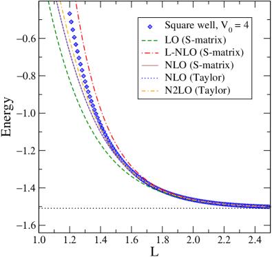
Figure 2: (color online) Bound-state energy for a square well of depth $V_{0}=4$ (lengths are in units of $R$ and energies in units of $1/R^{2}$ with $\hbar^{2}/\mu=1$) from solving the Schrödinger equation with a Dirichlet boundary condition at $r=L$. The diamonds are exact results for each $L$ while the horizontal dotted line is the energy for $L\rightarrow\infty$, $E_{\infty}=-1.5088$. The dashed, dot-dashed and solid lines are predictions for the energy using the systematic correction formula Eq. (17) at LO (first term only), L-NLO (first two terms), and full NLO (all terms), respectively. The dotted curve on top of the solid line and the dot-double-dashed lines are respectively the NLO and N2LO predictions for the square well from the Taylor expansion method described in Sec. II.2.

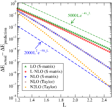
Figure 3: (color online) Error plots of the energy correction at each $L$ for the square well of Fig. 2 ($V_{0}=4$) predicted at different orders by Eq. (17) and by the Taylor expansion method in Sec. II.2, each compared to the exact energy. Lines proportional to $Le^{-4k_{\infty}L}$ (dashes) and $L^{2}e^{-6k_{\infty}L}$ (with arbitrary normalization) are plotted for comparison to anticipated error slopes.

Figure 2 compares the energy corrections for the general S-matrix method at LO and NLO for a representative square-well potential with one bound state to the exact energies. The Taylor expansion results for the square well at NLO and N2LO (which is proportional to $e^{-6k_{\infty}L}$) are also plotted. We note that the predictions are systematically improved as higher-order terms are included and that keeping terms only up to L-NLO overestimates the energy correction. Also as seen in Fig. 2, the full NLO energy correction predicted by Eq. (17), with $w_{2}$ determined by Eq. (21), matches the ‘exact’ NLO result obtained by Taylor expansion. This confirms that Eq. (17) is indeed the complete energy correction at NLO.

To see if the errors decrease with the implied systematics, we plot the difference of actual energy corrections and the energy corrections predicted at different orders on a log-linear scale in Fig. 3. We observe that the errors successively decrease at each fixed $L$ as we go from LO to NLO to N2LO. The up triangles in Fig. 3 are $\Delta E_{\rm actual}-\Delta E_{\rm LO}$. From Eq. (17) the dominant omitted correction in $\Delta E_{\rm LO}$ is proportional to $Le^{-4k_{\infty}L}$. As seen in Fig. 3, the slope of $\Delta E_{\rm actual}-\Delta E_{\rm LO}$ is roughly $Le^{-4k_{\infty}L}$, as expected. We also note that $\Delta E_{\rm\text{L-NLO}}$ is only a marginal improvement over $\Delta E_{\rm LO}$ for the plotted range of $L$ and that $\Delta E_{\rm actual}-\Delta E_{\rm NLO}$ has the expected slope of $L^{2}e^{-6k_{\infty}L}$. We again see a perfect agreement between the results obtained from the S-matrix method (17) and those obtained from the Taylor expansion of Eq. (22). We have also studied deeper square wells with more than one bound state and verified that the S-matrix approach applies to all the bound states.

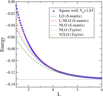
Figure 4: (color online) Bound-state energy for a square well of depth $V_{0}=1.83$ (units with $R=1$), which simulates a deuteron, from solving the Schrödinger equation with a Dirichlet boundary condition at $r=L$. The horizontal dotted line is the exact energy, $E_{\infty}=-0.1321$ and the other curves are as the same as in Fig. 2.

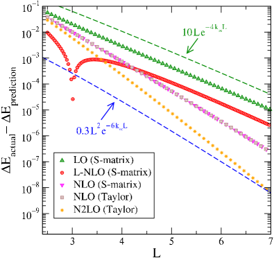
Figure 5: (color online) Comparison of the actual energy correction due to truncation to the energy correction predicted to different orders by Eq. (17) for a square well (Eq. (19)) with $V_{0}=1.83$ and $R=1$.

In Figs. 4 and 5, the same analysis is done but now with the depth of the square well adjusted so that the exact binding energy is the same as the deuteron binding energy scaled to the units $\hbar=1$, $\mu=1$ and $R=1$. An important difference in this case compared to the deeper square well is that the L-NLO prediction gives a very close estimate for the truncated energies at smaller $L$ values. However, the small errors in this region should not be over-emphasized because they are not systematic. As seen in Fig. 5, $\Delta E-\Delta E_{\rm\text{L-NLO}}$ is the dominant NLO correction at large $L$ but still has about the same slope as $\Delta E-\Delta E_{\rm LO}$, reflecting the $L$-dependence of the remainder of the NLO correction. Only when the full NLO correction is included does the slope go to $L^{2}e^{-6k_{\infty}L}$.

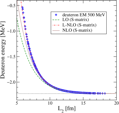
Figure 6: (color online) Deuteron energy versus $L_{2}$ (see Eq. (1)) for the chiral N³LO (500 MeV) potential of Ref. Entem and Machleidt (2003). To eliminate the UV contamination we only plot results for $\hbar\Omega>49$ MeV. The dashed, dot-dashed and solid lines are respectively the LO (first term in Eq. (17)), L-NLO (first two terms in Eq. (17)) and the full NLO (all the terms in Eq. (17)) predictions for the energy correction. The horizontal dotted line is the deuteron energy.

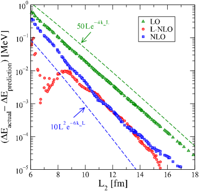
Figure 7: (color online) Comparison of the actual energy correction due to HO basis truncation ($\hbar\Omega$ restricted to be greater than $49$ MeV to eliminate UV contamination) for the deuteron to the energy correction predicted to different orders from Eq. (17). For the parameter $w_{2}$ in Eq. (17) we use the value reported in Phillips et al. (2000).

Figures 6 and 7 show analogous results for the deuteron calculated with the chiral EFT potential of Ref. Entem and Machleidt (2003). We use the HO basis and predict the ($l=0$) energy correction from Eq. (17) assuming a Dirichlet bc at $L_{2}$ given by Eq. (1). We only include energies for which $\hbar\Omega>49$ MeV, which is sufficient to render UV corrections negligible. For the parameter $w_{2}$ in Eq. (17) we use $w_{2}=0.389$ as reported in Phillips et al. (2000). We also note that the $\rho_{d}$ value reported in Phillips et al. (2000) satisfies Eq. (15), where $\gamma_{\infty}$ now is the $s$-wave ANC. The $y$-axis minimum is dictated by the limited precision of the ANC and $w_{2}$ values. We notice again that the close agreement of the L-NLO prediction to the deuteron data is not systematic while the full corrections to the LO and NLO predictions have the anticipated slopes except at large $L_{2}$. In the next Section we extend our formulas to $l>0$, which enables us to include contributions from the $d$-wave at LO. This becomes noticable on the error plot for large $L_{2}$ (see Fig. 9).

III Extension to nonzero orbital angular momentum

The deuteron ground state is a mixture of an $s$ and a $d$ state, and the $s$ and $d$ asymptotic normalization coefficients (as well as the $d$-to-$s$ state ratio of about 2.5%) are observables. The extrapolation formulas in the previous Section were derived for $s$ states, and it is of interest to extend these to nonzero angular momenta $l$. We do so in two steps. First, we show that $L_{2}$ is also the relevant effective hard-wall radius for oscillator wave functions with nonzero angular momenta. Second, we derive the energy correction for nonzero angular momenta.

III.1 $L$ for nonzero angular momenta

For the derivation of the relevant IR length scale at $l>0$ we closely follow Ref. More et al. (2013). We compute the smallest eigenvalue $\kappa^{2}$ of the squared momentum operator $\hat{p}^{2}$ in a finite oscillator basis and identify $\kappa=x_{l}/L$ (with $x_{l}$ being the smallest positive zero of the spherical Bessel function $j_{l}$). This identification, and the form of the corresponding eigenfunctions are, of course, guided by the Dirichlet bc at $r=L$. Throughout this Section, we set the oscillator length $b=1$. Because this is the only length scale here, the results are general and can be extended to any $b$ with a simple rescaling. The normalized radial oscillator wave function of energy

$$E=2n+l+3/2$$ (26)

is $\psi_{nl}(r)=u_{nl}(r)/r$ with

$$u_{nl}(r)=\sqrt{2n!\over\Gamma(n+l+3/2)}r^{l+1}e^{-r^{2}/2}L_{n}^{l+1/2}(r^{2})\;.$$ (27)

Here, $L_{n}^{l+1/2}$ denotes the generalized Laguerre polynomial.

In this basis, the operator $\hat{p}^{2}$ of the momentum squared is tridiagonal with matrix elements

$$\langle u_{ml}|\hat{p}^{2}|u_{nl}\rangle =(2n+l+3/2)\delta_{m}^{n}$$

$$\qquad\hbox{}+\sqrt{n+1}\sqrt{n+l+3/2}\,\delta_{m}^{n+1}$$

$$\qquad\hbox{}+\sqrt{n}\sqrt{n+l+1/2}\,\delta_{m}^{n-1}\;.$$ (28)

For the eigenfunction of $\hat{p}^{2}$ with smallest eigenvalue $\kappa^{2}$ at angular momentum $l$, we make the ansatz $\psi_{\kappa l}(r)/r$ with

$$\psi_{\kappa l}(r)=\left\{\begin{array}[]{cc}\kappa rj_{l}(\kappa r)\;,&0\leq\kappa r\leq x_{l}\;,\\ 0\;,&\kappa r>x_{l}\;.\end{array}\right.$$ (31)

Here, $j_{l}$ is the regular spherical Bessel function and $x_{l}$ is its smallest positive zero. Clearly, these eigenfunctions are those of a particle in a spherical cavity with a Dirichlet bc at $x_{l}/\kappa$. In an infinite basis, the wave function $\psi_{\kappa l}(r)/r$ is an eigenfunction of $\hat{p}^{2}$ for any non-negative value of $\kappa$. In a finite oscillator basis, only discrete momenta $\kappa$ are allowed. For their computation we expand the eigenfunction as

$$\psi_{\kappa l}(r)=\sum_{m=0}^{n}c_{m}(\kappa)u_{ml}(r)\;,$$ (32)

where we supress the dependence of the admixture coefficients $c_{m}(\kappa)$ on $l$, which is kept fixed throughout this derivation.

The last row of the matrix eigenvalue problem for $\hat{p}^{2}$ is

$$(2n+l+3/2-\kappa^{2})c_{n}(\kappa)=-\sqrt{n}\sqrt{n+l+1/2}\,c_{n-1}\;,$$ (33)

and this becomes the quantization condition for $\kappa$. The direct computation of the coefficients $c_{n}(\kappa)$ seems difficult. Instead, we make a Fourier-Bessel expansion

$$\psi_{\kappa l}(r)=\sqrt{2\over\pi}\int\limits_{0}^{\infty}\!dk\,\tilde{\psi}_{\kappa l}(k)\,krj_{l}(kr)\;,$$ (34)

and use

$$krj_{l}(kr)=\sqrt{\pi\over 2}\sum_{n=0}^{\infty}(-1)^{n}u_{nl}(k)u_{nl}(r)\;.$$ (35)

Thus,

$$\psi_{\kappa l}(r)=\sum_{n=0}^{\infty}(-1)^{n}u_{nl}(r)\int\limits_{0}^{\infty}\!dk\,\tilde{\psi}_{\kappa l}(k)u_{nl}(k)\;,$$ (36)

and the admixture coefficients are therefore

$$c_{n}(\kappa)=(-1)^{n}\int\limits_{0}^{\infty}dk\,\tilde{\psi}_{\kappa l}(k)u_{nl}(k)\;.$$ (37)

So far, our formal manipulations have been exact. We now employ an asymptotic approximation of the generalized Laguerre polynomials (which enters the $u_{nl}(k)$) in terms of Bessel functions, valid for $n\gg 1$, see Eq. (15) of Ref. Deaño et al. (2013). This yields

$$u_{nl}(k) \approx{2^{1-n}\over\pi^{1/4}}\sqrt{(2n+2l+1)!\over(n+l)!n!}\,(4n+2l+3)^{-{l+1\over 2}}$$

$$\qquad\hbox{}\times\sqrt{4n+2l+3}k\,j_{l}(\sqrt{4n+2l+3}k)\;,$$ (38)

and

$$c_{n}(\kappa) \approx C_{nl}\sqrt{2\over\pi}\int\limits_{0}^{\infty}dk\,\tilde{\psi}_{\kappa l}(k)\sqrt{4n+2l+3}k$$

$$\qquad\qquad\qquad\hbox{}\times j_{l}(\sqrt{4n+2l+3}k)\;.$$ (39)

Here, $C_{nl}$ is a constant that does not depend on $\kappa$. The key point is that the asymptotic expansion in terms of Bessel functions allows us now to employ the definition (34) to evaluate the integral

$$\sqrt{2\over\pi}\int\limits_{0}^{\infty}dk\, \tilde{\psi}_{\kappa l}(k)\sqrt{4n+2l+3}k\,j_{l}(\sqrt{4n+2l+3}k)$$

$$=\psi_{\kappa l}(\sqrt{4n+2l+3})$$

$$=\sqrt{4n+2l+3}\,\kappa\,j_{l}(\sqrt{4n+2l+3}\kappa)\;.$$ (40)

Putting it all together, we find

$$c_{n}(\kappa) ={2^{1/2-n}(-1)^{n}\pi^{1/4}\over(4n+2l+3)^{l/2}}\sqrt{(2n+2l+1)!\over(n+l)!n!}$$

$$\qquad\hbox{}\times\kappa\,j_{l}(\sqrt{4n+2l+3}\kappa)\;.$$ (41)

We insert this expression for $c_{n}(\kappa)$ into the quantization condition (33) and make the ansatz

$$\kappa={x_{l}\over\sqrt{4n+2l+3+2\Delta}}\ .$$ (42)

Assuming the limit $n\gg 1$ and $n\gg l$ in the quantization condition then yields

$$\Delta=2\ .$$ (43)

Thus, $\Delta$ does not depend on $l$ in this limit, and the result is consistent with the $l=0$ result of Ref. More et al. (2013). In other words, the extent of the position space in finite oscillator basis with maximum radial quantum number $n$ and angular momentum $l$ is

$$L_{2} = \sqrt{2(2n+l+3/2+2)}b$$ (44)

$$= \sqrt{2(N+3/2+2)}b\;,$$

in accord with Eq. (1).

Table 1 shows numerical comparisons for $l=0,1,2$ and a range of $n$ of the exact minimum momentum $\kappa$ and the estimate $x_{l}/L_{2}$ (with $x_{0}=\pi$, $x_{1}\approx 4.49341$, $x_{2}\approx 5.76346$). The estimates are accurate approximations of the exact results even for small $N=2n+l$, but the accuracy decreases somewhat with increasing orbital angular momentum. In some practical calculations it might thus be of advantage to directly employ the numerical results for $L_{2}$ instead of the approximate analytical expression (44).

Table 1: Comparison of the exact lowest momentum $\kappa$ with the analytical estimate $x_{l}/L_{2}$ for $l=0,1,2$ and $0\leq n\leq 10$.

$l$	$n$	$\kappa$	${x_{l}/L_{2}}$	$l$	$n$	$\kappa$	${x_{l}/L_{2}}$	$l$	$n$	$\kappa$	${x_{l}/L_{2}}$
0	0	1.2247	1.1874	1	0	1.5811	1.4978	2	0	1.8708	1.7378
0	1	0.9586	0.9472	1	1	1.2764	1.2463	2	1	1.5423	1.4881
0	2	0.8163	0.8112	1	2	1.1047	1.0898	2	2	1.3509	1.3222
0	3	0.7236	0.7207	1	3	0.9892	0.9805	2	3	1.2191	1.2018
0	4	0.6568	0.6551	1	4	0.9042	0.8987	2	4	1.1207	1.1092
0	5	0.6058	0.6046	1	5	0.8382	0.8344	2	5	1.0432	1.0352
0	6	0.5651	0.5642	1	6	0.7850	0.7822	2	6	0.9801	0.9742
0	7	0.5316	0.5310	1	7	0.7408	0.7387	2	7	0.9274	0.9229
0	8	0.5035	0.5031	1	8	0.7033	0.7018	2	8	0.8824	0.8789
0	9	0.4795	0.4791	1	9	0.6711	0.6698	2	9	0.8435	0.8407
0	10	0.4585	0.4582	1	10	0.6429	0.6419	2	10	0.8093	0.8070

III.2 Energy correction for finite angular momentum

Let us extend our $l=0$ result for $[\Delta E]_{\rm LO}$ to $l>0$ following the method in Sec. II. For orbital angular momentum $l$, the asymptotic wave function is

$$u_{L}(r)\overset{r\gg R}{\longrightarrow}k_{L}r\Bigl{(}h_{l}^{(1)}(ik_{L}r)-{h_{l}^{(1)}(ik_{L}L)\over h_{l}^{(1)}(-ik_{L}L)}h_{l}^{(1)}(-ik_{L}r)\Bigr{)}\;.$$ (45)

Here, $h_{l}^{(1)}$ denotes the spherical Hankel function of the first kind (or the spherical Bessel function of the third kind) Abramowitz and Stegun (1972). By definition $u_{L}(L)=0$.

In complete analogy to the case of $s$ waves (e.g., using (6) and (7) for general $l$), the correction $\Delta E$ of the energy at leading order is

$$[\Delta E]_{\rm LO}=-k_{\infty}\left(\gamma_{\infty}^{(l)}\right)^{2}{h_{l}^{(1)}(ik_{L}L)\over h_{l}^{(1)}(-ik_{L}L)}\ .$$ (46)

We note that

$${h_{l}^{(1)}(ix)\over h_{l}^{(1)}(-ix)}\approx-e^{-2x}$$ (47)

for $x\gg 1$. In particular, for $l=1$

$$[\Delta E]_{\rm LO}=k_{\infty}\left(\gamma_{\infty}^{(1)}\right)^{2}{k_{\infty}L+1\over k_{\infty}L-1}\,e^{-2k_{\infty}L}\;,$$ (48)

and for $l=2$

$$[\Delta E]_{\rm LO}=k_{\infty}\left(\gamma_{\infty}^{(2)}\right)^{2}{(k_{\infty}L)^{2}+3k_{\infty}L+3\over(k_{\infty}L)^{2}-3k_{\infty}L+3}\,e^{-2k_{\infty}L}\;.$$ (49)

These correction formulas are tested in Fig. 8. For coupled channels, the leading energy correction will be the sum of the LO corrections for the individual angular momenta. We note that lattices with periodic bc lead to energy shifts that depend on the angular momentum Koenig et al. (2011). In contrast, the basis truncations we consider in this work are variational and thus always yield a positive energy correction.

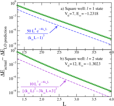
Figure 8: (color online) Error plots of the energy correction at each $L$ for a) $l=1$ and b) $l=2$ square-well states predicted at leading order by Eqs. (48) and (49) compared to the exact energy. Lines proportional to the expected L-NLO residual errors are plotted for comparison.

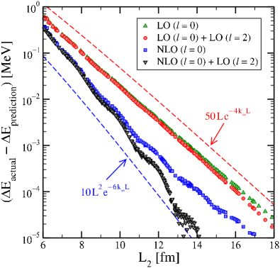
Figure 9: (color online) Residual error for the deuteron energy due to HO basis truncation as a function of $L=L_{2}$ (with $\hbar\Omega>49$ MeV to eliminate UV contamination) after subtracting $l=0$ energy corrections at different orders from Eq. (17) and the $l=2$ correction from Eq. (49). For the parameter $w_{2}$ in Eq. (17) we use the value reported in Phillips et al. (2000).

We return to the deuteron and take $|\gamma_{\infty}^{(2)}/\gamma_{\infty}^{(0)}|\approx 0.0226/0.8843$ from Ref. Machleidt and Entem (2011). Then

$$[\Delta E]_{\rm LO}=k_{\infty}\left(\gamma_{\infty}^{(0)}\right)^{2}e^{-2k_{\infty}L}$$ (50)

$$\qquad\hbox{}\times\left[1+\left|\frac{\gamma_{\infty}^{(2)}}{\gamma_{\infty}^{(0)}}\right|^{2}\frac{(k_{\infty}L)^{2}+3k_{\infty}L+3}{(k_{\infty}L)^{2}-3k_{\infty}L+3}\right]\;.$$

This formula is tested in Fig. 9 with the same deuteron calculations as in Fig. 7. We note that the deviation after subtraction of the NLO ($l=0$) result does not exhibit the $\exp(-6k_{\infty}L)$ falloff but is rather consistent with an $\exp(-4k_{\infty}L)$ falloff at large $L$. We attribute this to the missing LO $d$-state correction. Due to the small value of the $d$-to-$s$ state ratio, the $d$-wave correction is small, but it makes a perceptible shift of the $s$-wave LO result. When added to the NLO $l=0$ correction, the large $L_{2}$ behavior of the error is brought somewhat closer in line with the predicted dependence of $L^{2}e^{-6k_{\infty}L}$. We note, however, that the NLO correction is not complete due to the missing $l=2$ correction.

IV Alternative methods

In this Section we briefly consider two alternative approaches to the expansion for $\Delta E_{L}$. The linear energy method Djajaputra and Cooper (2000) was used in Refs. Furnstahl et al. (2012); More et al. (2013) to derive the form of the expansion and the leading term. A modified correction to LO for shallow bound states was also suggested in Ref. More et al. (2013), but we have found that it is not part of a consistent expansion; we correct it here. The other method constructs the differential variation of the energy with $L$, which can be integrated to reproduce our present expansion.

IV.1 Linear energy method

The linear energy method is based on the observation that the regular radial solution $u_{E}(r)$ for energy $E$ has a smooth expansion about $E=E_{\infty}$ at fixed $r$, so that the wave function for $E=E_{L}$, which is denoted $u_{L}(r)$, can be approximated by

$$u_{L}(r)\approx u_{\infty}(r)+\Delta E_{L}\left.\frac{du_{E}(r)}{dE}\right|_{E_{\infty}}+\mathcal{O}(\Delta E_{L}^{2})\;,$$ (51)

for $r\leq L$. By evaluating at $r=L$ with the boundary condition $u_{L}(L)=0$, $\Delta E_{L}$ is estimated as

$$\Delta E_{L}\approx-u_{\infty}(L)\left(\left.\frac{du_{E}(L)}{dE}\right|_{E_{\infty}}\right)^{-1}\;.$$ (52)

The leading approximation to $du_{E}(L)/dE|_{E_{\infty}}$ then leads to the LO result $\Delta E_{L}\propto e^{-2k_{\infty}L}$ with the coefficient correctly identified in Ref. More et al. (2013).

The modified energy correction proposed in Ref. More et al. (2013),

$$(\Delta E_{L})_{\rm mod}=k_{\infty}\gamma_{\infty}^{2}\frac{e^{-2k_{\infty}L}}{(1-\gamma_{\infty}^{2}Le^{-2k_{\infty}L})}\;,$$ (53)

contains all orders in the expansion factor $e^{-2k_{\infty}L}$. However, if expanded in a power series it does not reproduce correctly the $L$-dependent $e^{-4k_{\infty}L}$ term in Eq. (17). In light of the consistent expansion presented in this paper, it is clear that a term of $\mathcal{O}(L\gamma_{\infty}^{2}e^{-4k_{\infty}L})$ also arises from the $\mathcal{O}(\Delta E_{L}^{2})$ term in Eq. (51). When this contribution is taken into account the result from $(\Delta E_{L})_{\rm mod}$ matches that from Eqs. (17) up to L-NLO.

IV.2 Differential method

Because we seek the change in energy with respect to a cutoff, it is natural to formulate the problem in the spirit of renormalization group methods by seeking a flow equation for the bound-state energy as a function of $L$. Such an approach is already documented in the literature, for example in Refs. Arteca et al. (1984) and Fernández and Castro (1981), and it provides us with an alternative method that does not directly reference the S-matrix. The basic equation is

$$\frac{\partial E_{L}}{\partial L}=-\frac{1}{2}\frac{|u^{\prime}_{L}(L)|^{2}}{\int_{0}^{L}|u_{L}(r)|^{2}\,dr}\;.$$ (54)

Here the prime denotes a derivative with respect to $r$. Given an expression for the right-hand side in terms of observables ($k_{\infty}$, $\gamma_{\infty}$, and so on) and $L$, we can simply integrate to find the energy correction for a bc at $L$

$$\Delta E_{L}\equiv E_{L}-E_{\infty}=\int_{E_{\infty}}^{E_{L}}\!dE\,=\int_{\infty}^{L}\!\frac{\partial E_{L}}{\partial L}dL\;.$$ (55)

To derive Eq. (54), we start with

$$\frac{\partial}{\partial L}\left[\int_{0}^{L}u_{L}(r)Hu_{L}(r)\,dr=E_{L}\int_{0}^{L}\!dr\,u_{L}(r)^{2}\right]\;,$$ (56)

which yields (after some cancellations)

$$\frac{1}{2}\left.\left(\frac{\partial u_{L}(r)}{\partial r}\frac{\partial u_{L}(r)}{\partial L}\right)\right|_{0}^{L}=\frac{\partial E_{L}}{\partial L}\int_{0}^{L}\!dr\,u_{L}(r)^{2}\;.$$ (57)

The left-hand side is a surface term from partially integrating the kinetic energy in $H$. The lower limit vanishes because $u_{L}(0)=0$ for any $L$. Finally, we replace the partial derivative with respect to $L$ at the upper limit using

$$\frac{\partial u_{L}(L)}{\partial L}=-\frac{\partial u_{L}(L)}{\partial r}\;,$$ (58)

which follows from expanding $u_{L^{\prime}}(L^{\prime})=0$ about $u_{L}(L)=0$ for $L^{\prime}=L+\Delta L$.

To apply Eq. (54), we start with $u_{L}(r)$ in the asymptotic region, as given by Eq. (2). The normalization constant $\gamma_{L}$ is chosen so that the integral of $u_{L}(r)^{2}$ from 0 to $L$ is unity; it becomes the ANC $\gamma_{\infty}$ as $L\rightarrow\infty$. Thus

$$u_{L}^{\prime}(L)=-2\gamma_{L}k_{L}e^{-k_{L}L}\;.$$ (59)

Now we need to expand $k_{L}$ and $\gamma_{L}$ about $k_{\infty}$ and $\gamma_{\infty}$, respectively. The leading term is trivial: $k_{L}\rightarrow k_{\infty}$ and $\gamma_{L}\rightarrow\gamma_{\infty}$, so the only $L$ dependence in $u_{L}^{\prime}(L)^{2}$ is in $e^{-2k_{\infty}L}$ and the integration in (54) is immediate:

$$\Delta E_{L} =\int_{\infty}^{L}\!\frac{\partial E_{L}}{\partial L}dL=-2\gamma_{\infty}^{2}k_{\infty}^{2}\int_{\infty}^{L}\!e^{-2k_{\infty}L}\,dL$$

$$=k_{\infty}\gamma_{\infty}^{2}e^{-2k_{\infty}L}+\mathcal{O}(e^{-4k_{\infty}L})\;.$$ (60)

This is the same LO result for $\Delta E_{L}$ found by other methods. It is straightforward to extend this construction to $l>0$, reproducing Eq. (46).

To go to NLO we need an expression for $\gamma_{L}$. In the zero-range (zr) limit, $\gamma_{L}$ is given completely in terms of $k_{L}$ using the normalization condition (because the asymptotic form in Eq. (2) holds over the entire range of the integral)

$$\gamma_{L}^{2} =\left[\int_{0}^{L}\!dr\,(e^{-k_{L}r}-e^{-2k_{L}L}e^{k_{L}r})^{2}\right]^{-1}$$

$$=2k_{L}(1+4k_{L}Le^{-2k_{L}L})+\mathcal{O}(e^{-4k_{L}L})\;.$$ (61)

We expand $k_{L}$ everywhere in Eq. (54) using Eq. (59) and our LO result

$$k_{L}=k_{\infty}(1-2e^{-2k_{\infty}L})\;.$$ (62)

Here, we neglected terms that are $\mathcal{O}(e^{-6k_{\infty}L})$ or smaller. We need to expand $e^{-2k_{L}L}$ in $u_{L}^{\prime}(L)$ to get

$$e^{-2k_{L}L}=e^{-2k_{\infty}L}(1+4k_{\infty}Le^{-2k_{\infty}L})+\mathcal{O}(e^{-6k_{\infty}L})\;.$$ (63)

(Elsewhere it suffices to replace $e^{-2k_{L}L}$ by $e^{-2k_{\infty}L}$ to NLO.) So we find that

$$\frac{\partial E_{L}}{\partial L} =-\frac{1}{2}(4\gamma_{L}^{2}k_{L}^{2}e^{-2k_{L}L})$$

$$\approx-2[2k_{\infty}(1-2e^{-2k_{\infty}L})(1+4k_{\infty}Le^{-2k_{\infty}L})]$$

$$\ \hbox{}\times[k_{\infty}^{2}(1-4e^{-2k_{\infty}L})][e^{-2k_{\infty}L}(1+4k_{\infty}Le^{-2k_{\infty}L})]$$

$$\approx-4k_{\infty}^{3}e^{-2k_{\infty}L}-8k_{\infty}^{3}(4k_{\infty}L-3)e^{-4k_{\infty}L}$$

$$\qquad\hbox{}+\mathcal{O}(e^{-6k_{\infty}L})\;,$$ (64)

and then finally

$$[\Delta E_{L}]_{\rm zr,NLO} =\int_{\infty}^{L}\!\frac{\partial E_{L}}{\partial L}dL$$

$$=2k_{\infty}^{2}e^{-2k_{\infty}L}+4k_{\infty}^{2}(2k_{\infty}L-1)e^{-4k_{\infty}L}$$

$$\qquad\hbox{}+\mathcal{O}(e^{-6k_{\infty}L})\;,$$ (65)

in agreement with Eq. (17) with $\gamma_{\infty}^{2}=2k_{\infty}$ and $w_{2}=0$. We can take this procedure to higher order by using a more general expansion for $k_{L}$.

To extend the differential method to higher order for nonzero range, we must parametrize $\gamma_{L}$ to account for the part of the integration within the range of the potential; e.g., in terms of the effective range. However, we have not found a clear advantage in doing this compared to the straightforward S-matrix method.

V Radii

In this Section, we compute corrections to the radius for $l=0$ to $\mathcal{O}(e^{-2k_{\infty}L})$. The corresponding formula was given in Ref. Furnstahl et al. (2012) without a derivation. We define

$$\langle r^{2}\rangle_{L}=\langle r^{2}\rangle_{\infty}+\Delta\langle r^{2}\rangle_{L}\;,$$ (66)

where

$$\Delta\langle r^{2}\rangle_{L}=\frac{\int_{0}^{L}|u_{L}(r)|^{2}\,r^{2}\,dr}{\int_{0}^{L}|u_{L}(r)|^{2}\,dr}-\frac{\int_{0}^{\infty}|u_{\infty}(r)|^{2}\,r^{2}\,dr}{\int_{0}^{\infty}|u_{\infty}(r)|^{2}\,dr}\;.$$ (67)

Though the squared radius is a long-ranged operator, its matrix elements will still be modified at short distances by renormalizations or similarity transformations of the Hamiltonian, see, e.g., Ref. Stetcu et al. (2005). Thus we cannot expect an extrapolation law for the radius that depends entirely on observables. Instead, we seek a formula that identifies the $L$ dependence but leaves parameters to be fit.

The strategy is to isolate the polynomial $L$ dependence by splitting the necessary integrals into an interior part and an exterior part:

$$\int_{0}^{L}\!r^{n}|u_{L}(r)|^{2}\,dr=\int_{0}^{R}\!r^{n}|u_{L}(r)|^{2}\,dr+\int_{R}^{L}\!r^{n}|u_{L}(r)|^{2}\,dr\;,$$ (68)

where $R$ is sufficiently large so that the asymptotic form of $u_{L}(r)$ from Eq. (2) can be used in the second integral. Our expression for $\Delta\langle r^{2}\rangle_{L}$ is independent of the normalization of $u_{L}(r)$, so we are free to choose it so that the large $r$ form is exactly given by Eq. (2).

The first integral will depend on the details of the interior wave function and therefore on the potential, but the linear energy method shows us that to $\mathcal{O}(e^{-2k_{\infty}L})$ the $L$ dependence is isolated. In particular, the dependence on $L$ of $u_{L}(r)$ in Eq. (51) is confined to $\Delta E_{L}=k_{\infty}\gamma_{\infty}^{2}e^{-2k_{\infty}L}$ because $du_{E}(r)/dE|_{E_{\infty}}$ for $r<R$ is independent of $L$ with our choice of normalization. Thus the integral over $r$ cannot introduce polynomial $L$ dependence and we can conclude that

$$\int_{0}^{R}\!r^{n}|u_{L}(r)|^{2}\,dr=\mathcal{O}(L^{0})e^{-2k_{\infty}L}+\mathcal{O}(e^{-4k_{\infty}L})\;.$$ (69)

The $\mathcal{O}(L^{0})$ coefficient will depend on the potential, so we will treat it as a parameter to be fit.

The second integral can be directly evaluated to $\mathcal{O}(e^{-2k_{\infty}L})$ using Eq. (2) and $[k_{L}]_{LO}=k_{\infty}-\gamma_{\infty}^{2}e^{-2k_{\infty}L}$ to expand $|u_{L}(r)|^{2}$. For $n=0$ we find

$$\int_{R}^{L}\! |u_{L}(r)|^{2}\,dr=\frac{1}{2k_{\infty}}e^{-2k_{\infty}R}$$

$$\hbox{}+\Bigl{[}\frac{\gamma_{\infty}^{2}}{k_{\infty}}\Bigl{(}R+\frac{1}{2k_{\infty}}\Bigr{)}e^{-2k_{\infty}R}+2R-2L\Bigr{]}e^{-2k_{\infty}L}$$

$$\hbox{}+\mathcal{O}(e^{-4k_{\infty}L})\;,$$ (70)

and for $n=2$ we find

$$\int_{R}^{L}\! r^{2}|u_{L}(r)|^{2}\,dr=\frac{1}{2k_{\infty}^{3}}\Bigl{[}\frac{1}{2}+k_{\infty}R+(k_{\infty}R)^{2}\Bigr{]}e^{-2k_{\infty}R}$$

$$\hbox{}+\Bigl{[}\frac{\gamma_{\infty}^{2}}{k_{\infty}^{4}}\Bigl{(}\frac{3}{4}+\frac{3}{2}k_{\infty}R+\frac{3}{2}(k_{\infty}R)^{2}+(k_{\infty}R)^{3}\Bigr{)}e^{-2k_{\infty}R}$$

$$\qquad\hbox{}+\frac{1}{k_{\infty}^{3}}\Bigl{(}\frac{2}{3}(k_{\infty}R)^{3}-k_{\infty}L-\frac{2}{3}(k_{\infty}L)^{3}\Bigr{)}\Bigr{]}e^{-2k_{\infty}L}$$

$$\hbox{}+\mathcal{O}(e^{-4k_{\infty}L})\;.$$ (71)

Note that it is necessary to keep the expansion of $|u_{L}(r)|^{2}$ up to $e^{-4k_{\infty}L}$ until after doing the integrals because terms proportional to $e^{-4k_{\infty}L}e^{2k_{\infty}r}$ will be leading order.

When we use (70) and (71) and our previous result for the interior integrals in Eq. (67), expanding consistently to $\mathcal{O}(e^{-2k_{\infty}L})$, we will mix $R$-dependent terms with the $L$ dependence. However, we can immediately conclude that the general form to this order is (with $\beta\equiv 2k_{\infty}L$)

$$\langle r^{2}\rangle_{L}\approx{\langle r^{2}\rangle_{\infty}}[1-(c_{0}\beta^{3}+c_{1}\beta+c_{2})e^{-\beta}]\;.$$ (72)

Here, $\langle r^{2}\rangle_{\infty}$, $c_{0}$, $c_{1}$, and $c_{2}$ are fit parameters while $k_{\infty}$ should be determined from fitting the energy. This form has been verified explicitly for finite-range model potentials (e.g., square well and delta shell). The approximation (72) should be valid in the asymptotic regime $\beta\gg 1$. In practice, for a robust extrapolation one needs $\beta$ large enough so that the $\beta^{3}$ correction dominates the subleading terms.

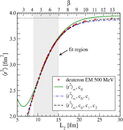
Figure 10: (color online) Deuteron radius squared versus $L_{2}$ for the chiral N³LO (500 MeV) potential of Ref. Entem and Machleidt (2003). To eliminate the UV contamination we only plot results for $\hbar\Omega>49$ MeV. The solid, dot-dashed, and dashed lines are results from fitting Eq. (72) in the shaded region to find $\langle r^{2}\rangle_{\infty}$ and one, two, or three of the $c_{i}$ constants, respectively. The horizontal dotted line is the deuteron radius squared.

If we take the zero-range limit $R\to 0$ of the potential, we arrive at the simple expression

$$\frac{\Delta\langle r^{2}\rangle_{L}}{\langle r^{2}\rangle_{\infty}}\approx-\left(\frac{(2k_{\infty}L)^{3}}{3}-4\right)e^{-2k_{\infty}L}\;.$$ (73)

Note that in this limit the correction becomes independent of the potential. Equation (73) suggests that for a short-range potential, the $c_{1}$ and $c_{2}$ terms will give comparable contributions for moderate $\beta$, and therefore will be difficult to determine reliably.

Sample fits of Eq. (72) for the deuteron are shown in Fig. 10. Results are given for fitting one, two, and all three $c_{i}$ constants to radii calculated with the same truncated oscillator basis parameters used for Fig. 6. The fit region is for $L_{2}$ between 9 and 15 fm, where the calculations only show a small amount of curvature. All points are equally weighted. The extrapolated radius squared $\langle r^{2}\rangle_{\infty}$ for the three cases are 3.95 fm², 3.87 fm², and 3.89 fm², compared to the exact result of 3.90 fm². If the fit region is instead taken between 11 and 17 fm, the corresponding results are 3.91 fm², 3.89 fm², and 3.90 fm². For all of these fits, the value of $c_{0}$ is fairly stable, ranging from 0.27 to 0.33 (note that $c_{0}=1/3$ in the zero-range limit). In contrast, $c_{1}$ and $c_{2}$ are not well determined (even the sign of $c_{1}$ varies). This is consistent with fits using the square-well potential, where analytic expressions for the $c_{i}$s can be found. We find that $\langle r^{2}\rangle_{\infty}$ and $c_{0}$ are well determined by fits in analogous regions but that $c_{1}$ and $c_{2}$ are not. If we push the analysis by taking the fit region between 7 and 13 fm, the $\langle r^{2}\rangle_{\infty}$ prediction using only $c_{0}$ breaks down, giving 4.21 fm². However, the fit with all three $c_{i}$s is still reasonable, giving 3.86 fm². Further studies are needed to test how these trends might carry over to $A>2$ nuclei.

The derivation given here can be directly extended to $l>0$ using the general expression for the asymptotic wave function in Eq. (45). However, this wave function has additional $L$ dependence so the corresponding result to Eq. (72) will have more complicated $\beta$ dependence unless additional simplifications are made. The extension to other single-particle coordinate-space operators is also direct, by replacing $r^{2}$ with the appropriate expression.

VI Summary and open questions

In this paper we derived and tested a consistent and systematic expansion for the $s$-wave binding momentum and energy of a two-body system with a Dirichlet boundary condition, Eqs. (16) and (17). As shown in Ref. More et al. (2013) for $l=0$ bound states, such a boundary condition arises as an effective infrared cutoff when using a truncated harmonic oscillator basis. Here we extended to $l>0$ the derivation from More et al. (2013) that associates the oscillator basis parameters to the appropriate hard-wall radius $L$. The same formula for $L$ derived previously for $l=0$ (called $L_{2}$) is found to still hold for general $l$ if expressed in terms of the oscillator quantum number $N=2n+l$. We subsequently obtained the energy correction for $l>0$ at LO.

Our expansion is based on the analytic structure of the two-body S-matrix in the complex momentum plane. The asymptotic wave functions for a boundary condition at $r=L$ are analytic continuations of the scattering solutions to (purely) imaginary momentum. If continued to $k=ik_{\infty}$, the free-space $L=\infty$ binding momentum, one reaches a pole of the S-matrix with residue determined by the asymptotic normalization $\gamma_{\infty}$. If there are no long-range interactions that generate intermediate singularities, as is the case for the deuteron where the one-pion exchange threshold is further away, this entire continuation is determined by measurable quantities (the on-shell S-matrix). The binding momentum $k_{L}$ for the boundary condition at $L$ is intermediate between zero and $k_{\infty}$ and therefore it is determined by observables.

The expansion for $k_{L}$ and subsequently $E_{L}$ is naturally formulated using an effective range expansion of $k\cot\delta_{l}(k)$ about the pole at $ik_{\infty}$. The expansion is in powers of $e^{-2k_{\infty}L}$ (LO goes like $e^{-2k_{\infty}L}$, NLO like $e^{-4k_{\infty}L}$, and so on), with prefactors that depend on $L$, $k_{\infty}$, $\gamma_{\infty}$, and higher-order effective range parameters. The leading term and the $L$-dependent NLO term are determined by the pole alone, while other NLO and higher-order terms require a valid parameterization of the S-matrix away from the pole. (For a zero-range interaction, the expansion depends on $k_{\infty}$ only.) This organization was tested for model potentials (not all shown here) and a realistic deuteron calculation (the latter within a harmonic oscillator basis). The use of semi-log error plots to compare to analytic results for the square well and to numerical results for the deuteron demonstrates the validity of the expansion over a wide range of $L$. We found the use of error plots to be a much more robust test than simply graphing the approach to $E_{\infty}$.

The use of a Dirichlet boundary condition is only an approximation to the actual asymptotic behavior of the harmonic oscillator basis in coordinate representation. However, as illustrated in Fig. 1, the difference in behavior is a high-momentum effect. Our error plots for the deuteron, which represent an indirect comparison because the energies were found from oscillator-truncated diagonalizations, suggest the former corrections remain subleading to the NLO corrections for $E_{L}$ over a wide range in $L$. We note that LO corrections due to the $d$-wave component of the deuteron are small but push the error plots to good agreement with the expected LO error proportional to $Le^{-4k_{\infty}L}$ at the largest $L$ values.

Two alternative derivations of the expansions for $k_{L}$ and $E_{L}$ were also presented, based on the linear energy method and a differential method, respectively. For the former, we corrected the modified version of the expansion for $E_{L}$ proposed in More et al. (2013), which was not consistent at $\mathcal{O}(e^{-4k_{\infty}L})$. While these alternatives provide different perspectives on the energy corrections, we did not find any new capabilities thus far. However, they may be more useful in calculations of other quantities (which can be scheme dependent); this is being explored.

The formulation in terms of S-matrix analytic structure is closely related to methods used to analyze break-up reactions, which provides a link to $A>2$ extrapolations. Indeed, in Ref. Furnstahl et al. (2012) the basic form of the LO extrapolation proportional to $e^{-2k_{\infty}L}$ was based on interpreting $k_{\infty}$ in terms of the one-particle separation energy. More generally, the asymptotic many-body wave function is dominated by configurations corresponding to the break-up channels with the lowest separation energies and it is their modification by the hard wall at $L$ that will be associated with the energy shift $\Delta E_{L}$. This is in turn dominantly described by the S-matrix near poles at the corresponding separation binding momenta. Future work will seek to clarify the precise nature of the more general expansion (including the effects of the Coulomb interaction) and whether it will be possible to quantitatively extract asymptotic normalization constants.

It might be challenging to derive NLO corrections to the binding energies for nuclei with $A>2$, particular for nuclei with nonzero ground-state spin. Here, many different orbital anglar momenta can contribute to the ground-state wave function, and one would presumably need to know the admixture of the different channels quite accurately. Our results show that nonzero orbital angular momenta yield corrections in inverse powers of $k_{\infty}L$ to the LO energy extrapolation. On the other hand, the leading contributions to bound-state energies in finite model spaces fall off as $\exp{(-2k_{\infty}L)}$ for all orbital angular momenta. This makes extrapolations feasible in practice.

Corrections due to the UV cutoff induced by a finite oscillator space were not considered in the present work, because the effective oscillator momentum cutoffs used (e.g., for the deuteron in Figs. 6, 7, and 9) were well above the intrinsic cutoff of the input potential. We have demonstrated that in this case the energy will be converged in the UV. However, rendering the UV correction negligible may not always be practical for larger systems with some methods Roth et al. (2013). This motivates, together with the success of phenomenological extrapolation schemes, a search for theoretically founded schemes that combine IR and UV expansions. Our systematic IR expansion relies on the IR cutoff being in the asymptotic region in coordinate space, beyond the range of the potential. The UV cutoff is at high momentum, however, where the potential is directly modified. While the duality of the oscillator Hamiltonian implies that the UV cutoff will be well approximated by a hard cutoff at a momentum given by the analogous expression to Eq. (1), the energy corrections will be dependent on the potential (i.e., not dependent only on observables). These issues will be explored in a forthcoming publication.