Tunneling Spectroscopy of a Spiral Luttinger Liquid in Contact with Superconductors

Abstract

One-dimensional wires with Rashba spin-orbit coupling, magnetic field, and strong electron-electron interactions are described by a spiral Luttinger liquid model. We develop a theory to investigate the tunneling density of states into a spiral Luttinger liquid under the proximity effect with superconductors. This approach provides a way to disentangle the delicate interplay between superconducting correlations and strong electron interactions. If the wire-superconductor boundary is dominated by Andreev reflection, we find that in the vicinity of the interface the zero-bias tunneling anomaly reveals a power law enhancement with the unusual exponent. Far away from the interface strong correlations inherent to the Luttinger liquid prevail and restore conventional suppression of the tunneling density of states at the Fermi level, which acquire, however, a Friedel-like oscillatory envelope with the period renormalized by the strength of the interaction.

I Introduction

In a one-dimensional system strong electron-electron interactions cause non-Fermi-liquid physics, which is described by the Luttinger liquid theory GiamarchiBook . Nowadays quantum wires with Rashba spin-orbit coupling in the external magnetic field attract a great deal of attention due to their special charge and spin transport, as well as spectral properties Streta03 ; Sun-PRL07 ; BrauneckerPRL09 ; Schuricht-PRB12 ; BrauneckerPRB12 ; Yacoby-ArXiv13 ; Loss-ArXiv13 ; Schmidt-ArXiv13 . The presence of spin-orbit coupling leads to a relative shift of the electronic dispersions for both spin species. Furthermore, a magnetic field applied to the system lifts the spin degeneracy and causes the opening of a Zeeman gap in the spectrum. If the chemical potential lies inside the gap, the system is equivalent to a spinful Luttinger liquid with a spiral magnetic field. This peculiar state was abbreviated as a spiral Luttinger liquid (SLL). In the presence of a bulk $s$-wave superconducting order, the wire becomes a topological superconductor and hosts Majorana zero energy modes Lutchyn10 ; Oreg10 . Compelling evidence for the latter has been recently reported in experiments kouwenhovenSCI12 ; Rokhinson12 ; deng12 ; das12 . It is obviously of great interest to investigate the fate of superconducting correlations when embedded into the environment of the strongly interacting Luttinger liquid. Previous works considered the phase diagram for this system in the presence of bulk superconductivity Gangadharaiah11 ; Sela11 ; Stoudenmire11 . Here we develop a theory for the spatially and energy resolved tunneling spectroscopy of a spiral Luttinger liquid which is brought into the proximity to a superconductor (SC) at its boundary. This proposal provides a way to disentangle the interplay between the complexity of the superconducting effects and the nontrivial electron liquid properties.

It is very well known from the context of mesoscopic conductors that if the normal wire is placed between two superconductors, thus forming a superconductor-normal-superconductor junction, its spectral properties are strongly affected by the proximity effect Proximity-Review . Indeed, the leakage of Cooper pairs into the wire induces a nonvanishing superconducting pair amplitude which opens a gap in the spectrum of the wire. For wires with a length exceeding the superconducting coherence length, the gap is small, of the order of Thouless energy $E_{Th}$, which evolves into the complete superconducting gap $\Delta$ in the opposite limit of short wires. If the normal wire is replaced by the Luttinger liquid conductor, then even without superconducting perturbations the density of states already has a striking feature. This is the famous zero-bias anomaly – the density of states vanishing as a power law near the Fermi energy. KF One may naively expect that proximitizing the Luttinger liquid with a superconductor would further facilitate depletion of the states near the Fermi energy towards opening a gap. Surprisingly, one discovers an entirely different scenario, an enhancement of the anomaly – the zero-bias peak – which physically can be rooted to the coherent backscattering from the interface of the subgap excitations that lead to the pileup of states near the zero energy Winkelholz96 . The latter has interesting consequences for the Josephson effect in the Luttinger liquid constriction between superconducting leads Maslov96 ; Fazio ; Smitha . A similar enhancement mechanism for tunneling has been also discussed for a Luttinger liquid with impurity Oreg-PRL96 . Here we study this physics in the context of spiral Luttinger liquids.

The behavior of the tunneling density of states (TDOS) is sensitive to the properties of the boundary between the Luttinger liquid and a superconductor. Competition between normal and Andreev reflection for this system has been discussed recently in the literature Fidkowski12 . We consider a perfect SC-SLL interface that is dominated by an Andreev boundary condition Winkelholz96 ; Maslov96 . By performing a canonical transformation to separate a gapless field from a gapped field, and using a mode expansion, we obtain the low-energy asymptote for the tunneling density of states analytically. We conclude that although Zeeman splitting and a Rashba interaction destroy the TDOS enhancement for the case when the chemical potential $\mu$ is detuned from the Zeeman gap, an enhancement survives in the SLL limit, namely, when $\mu$ lies within the gap. The power exponent of this anomaly is different as compared to that in the conventional case of a spinful Luttinger liquid without spin-orbit coupling. An enhancement manifests only for distances close to the SC-SLL interface in the wire, but disappears far away from the contact where strong correlations inherent to SLL restore conventional power law suppression of TDOS with additional oscillations. The latter contribution is reminiscent of Friedel oscillations with the period renormalized by interactions Ussishkin . We also compute the tunneling density of states numerically by using a self-consistent harmonic approximation and find the result to be consistent with the analytical calculations.

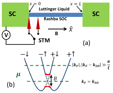
Figure 1: (a) Schematic representation of a superconductor-spiral Luttinger liquid wire system. (b) Band structure of the wire with Rashba spin-orbit coupling (SOC) and a magnetic field. The green dashed lines describe the position of the chemical potential $\mu$ for two different cases: (1) $|k_{F}|,\;|k_{F}-k_{\rm SO}|\gg 1/\xi$ for which $\mu$ is far above the Zeeman gap; (2) $k_{F}=k_{\rm SO}$ for which $\mu$ lays within the Zeeman gap.

II Model and Hamiltonian

We consider an interacting one-dimensional (1D) quantum wire with Rashba spin-orbit coupling in the $z$ direction and a magnetic field in parallel with the wire. Both sides of the wire are in perfect contact with an $s$-wave superconductor. We are interested in the density of states of the wire in the presence of electron-electron interactions. A schematic setup of the system under consideration is shown in Fig. 1(a). The Hamiltonian of the central part, i.e., the 1D Rashba wire with length $L$, can be written as

$$H_{\rm W}=\int_{0}^{L}dx\vec{\Psi}^{\dagger}(x)H(x)\vec{\Psi}(x)^{T}+\int_{0}^{L}dxdx^{\prime}U\rho(x)\rho(x^{\prime}),$$ (1)

with

$$H(x)=-\frac{\partial_{x}^{2}}{2m}+\mu+B\hat{\sigma}_{x}-i\frac{k_{\rm SO}}{m}\hat{\sigma}_{z}\partial_{x},$$ (2)

where $\vec{\Psi}^{\dagger}(x)=(\Psi_{\uparrow}^{\dagger}(x),\Psi_{\downarrow}^{\dagger}(x))$ being the electron annihilation operators for spin $s=\uparrow,\downarrow$ at position $x$, and $k_{\rm SO}$ is the Rashba spin-orbit momentum of the wire. The magnetic field is applied along the $x$ direction, and is assumed to be uniform. The second term in Eq. (1) represents the electron-electron interaction with potential $U(x-x^{\prime})$, and $\rho(x)=\sum_{s}\Psi_{s}^{\dagger}(x)\Psi_{s}(x)$ is the electron density (we choose $\hbar=1$ throughout the paper). It is convenient to perform a spin-dependent gauge transformation, $\Psi_{\uparrow\downarrow}(x)=\psi_{\uparrow\downarrow}(x)e^{\pm ik_{\rm SO}x}$, followed by a standard bosonization in a linearized spectrum:

$$\hskip-7.11317pt\psi_{\pm,s}(x)\!\! = \!\!\frac{1}{\sqrt{2\pi\alpha}}e^{i\sqrt{\frac{\pi}{2}}\Phi_{\pm,s}(x,t)}$$ (3)

$$= \!\!\frac{1}{\sqrt{2\pi\alpha}}e^{i\sqrt{\frac{\pi}{2}}\{\mp[\phi_{\rho}(x)+s\phi_{\sigma}(x)]+\theta_{\rho}(x)+s\theta_{\sigma}(x)\}}$$

with the full fermion operator $\psi_{s}(x)=e^{ik_{F}x}\psi_{+,s}(x)+e^{-ik_{F}x}\psi_{-,s}(x)$, where $\psi_{\pm,s}(x)$ represent the right and left moving fields, respectively, and $\alpha$ is a conventional short distance cutoff. Note that this transformation also shifts the chemical potential $\mu\rightarrow\mu+k_{\rm SO}^{2}/2m$. After these steps, the system is reduced to an equivalent spiral Luttinger liquid model, BrauneckerPRL09 ; BrauneckerPRB12 which is written in terms of bosonic spin ($\sigma$) and charge ($\rho$) fields and reads explicitly as

$$H_{\rm W}=\sum_{\nu=\rho,\sigma}\frac{v_{\nu}}{2}\int_{0}^{L}dx\left[g_{\nu}(\partial_{x}\theta_{\nu})^{2}+g^{-1}_{\nu}(\partial_{x}\phi_{\nu})^{2}\right]$$

$$+\frac{B}{2\alpha}\int_{0}^{L}dx\cos\left[\sqrt{2\pi}(\phi_{\rho}+\theta_{\sigma})-2(k_{F}-k_{\rm SO})x\right],$$ (4)

where $g_{\rho,\sigma}$ are the interaction parameters and $v_{\rho,\sigma}$ are the renormalized Fermi velocities. The fast oscillating terms on the scales $\sim 2k_{\rm SO}x$ and $\sim 2(k_{F}+k_{\rm SO})x$ are neglected in Eq. (4). We discuss two possible cases as shown in Fig. 1 (b): (1) $\mu$ is far above the Zeeman gap, i.e., $|k_{F}|,\;|k_{F}-k_{\rm SO}|\gg 1/\xi$ with the correlation length being the minimal scale between the wire length and thermal length $\xi=\mathrm{min}\{L,v_{F}/T\}$; (2) the chemical potential $\mu$ lies in the middle of the Zeeman gap, i.e., $k_{F}\approx k_{\rm SO}$. For case (1), the term proportional to $B$ strongly oscillates and thus is irrelevant in the renormalization group (RG) sense. Therefore, the magnetic field can be neglected in the low-energy limit from Eq. (4), and the model becomes the SC-spinful LL wire system with, however, an extra term, $\sim\int dx\cos[\sqrt{8\pi}\theta_{\sigma}]$, due to the pair hopping processes Sun-PRL07 . This term induces a spin gap and totally destroys the anomalous enhancement of TDOS. This behavior is in sharp contrast with the SC-spinful LL wire without spin-orbit physics involved Winkelholz96 . For case (2), the cosine is only slowly oscillating and such a spatial modulation that is due to $2(k_{F}-k_{\rm SO})x$ can be dropped out if $|k_{F}-k_{\rm SO}|<1/\xi$. In that limit, the magnetic field $B$ is relevant and will grow as energy decreases if $g_{\rho}+1/g_{\sigma}<2$ BrauneckerPRL09 ; BrauneckerPRB12 . Note that the pair hopping processes are strongly suppressed due to the Zeeman gap. We will mostly focus on case (2) in this paper.

III Mode expansion for Andreev boundary condition

We assume that the Rashba wire-superconductor interfaces are very clean such that the Andreev reflection is the dominant process at both boundaries. To treat the interfaces in the deep subgap limit, $\varepsilon\ll\Delta$ with SC gap $\Delta$, we apply the following fermion fields matching the condition Fidkowski12 ; Winkelholz96 ; Maslov96 $\psi_{+,s}(x=0,L)=\mp ie^{i\chi_{1,2}}\psi_{-,-s}^{\dagger}(x=0,L)$, where $s$ stands for spin-up and spin-down channels, respectively, and $\chi_{1,2}$ are the phases of the SC order for the left (near $x=0$) and right (near $x=L$) superconductors. It is important to emphasize that the spin-dependent gauge transformation used above to transform the Hamiltonian leaves invariant both the Cooper pairing term in the $s$-wave SC and the Andreev boundary condition. To proceed, we adopt the canonical mode expansion Winkelholz96 ; Maslov96

$$\theta_{\rho}(x)\!\! = \!\!\sqrt{\frac{\pi}{2}}(J+\chi)\frac{x}{L}+i\sqrt{\frac{1}{g_{\rho}}}\sum_{q>0}\gamma_{q}\sin(qx)(b_{\rho q}^{\dagger}-b_{\rho q}),$$

$$\theta_{\sigma}(x)\!\! = \!\!\frac{\theta_{\sigma}^{0}}{\sqrt{\pi}}+\sqrt{\frac{1}{g_{\sigma}}}\sum_{q>0}\gamma_{q}\cos(qx)(b_{\sigma q}^{\dagger}+b_{\sigma q}),$$

$$\phi_{\rho}(x)\!\! = \!\!\frac{\phi_{\rho}^{0}}{\sqrt{\pi}}+\sqrt{g_{\rho}}\sum_{q>0}\gamma_{q}\cos(qx)(b_{\rho q}^{\dagger}+b_{\rho q}),$$

$$\phi_{\sigma}(x)\!\! = \!\!\sqrt{\frac{\pi}{2}}M\frac{x}{L}+i\sqrt{g_{\sigma}}\sum_{q>0}\gamma_{q}\sin(qx)(b_{\sigma q}^{\dagger}-b_{\sigma q}),$$ (5)

where $\chi=\chi_{1}-\chi_{2}$ is the global phase difference between two SC islands, $b_{\rho q}$ and $b_{\sigma q}$ are bosonic operators, $\gamma_{q}=e^{-q\alpha/2\pi}/\sqrt{qL}$ is the convergence factor, and $q=\pi n/L$ ($n=1,2,...$). The zero mode operators, satisfying the commutations $[\theta_{\sigma}^{0},\,M]=i$ and $[\phi_{\sigma}^{0},\,J]=i$, describe the topological excitations Haldane . Note that those are not the eigenmodes for our system, and just serve as the starting point for the diagonalization later.

IV Low-energy TDOS of the wire

The magnetic field will flow to strong coupling for $g_{\rho}+1/g_{\sigma}<2$ at low energy. To separate the corresponding gapped field from a gapless part, one can apply the following canonical transformation: BrauneckerPRL09

$$\phi_{\rho}=\frac{g_{\rho}}{\sqrt{g}}\,\phi_{+}+\sqrt{\frac{g_{\rho}}{g_{\sigma}g}}\,\phi_{-}\,,\;\theta_{\rho}=\frac{1}{\sqrt{g}}\,\theta_{+}+\frac{1}{\sqrt{g_{\rho}g_{\sigma}g}}\,\theta_{-}$$

$$\phi_{\sigma}=\frac{1}{\sqrt{g}}\,\theta_{+}-\sqrt{\frac{g_{\rho}}{g_{\sigma}g}}\,\theta_{-}\,,\;\theta_{\sigma}=\frac{1}{g_{\sigma}\sqrt{g}}\,\phi_{+}-\sqrt{\frac{g_{\rho}}{g_{\sigma}g}}\,\phi_{-}\,,$$ (6)

where $g=g_{\rho}+1/g_{\sigma}$. The Hamiltonian (4) then becomes

$$H_{W} = \int_{0}^{L}dx\sum_{i=\pm}\frac{u_{i}}{2}\Big{[}(\partial_{x}\theta_{i})^{2}+(\partial_{x}\phi_{i})^{2}\Big{]}$$ (7)

$$+\frac{B}{2\alpha}\int_{0}^{L}dx\cos[\sqrt{2\pi g}\phi_{+}(x)],$$

where $u_{+}=(v_{\rho}g_{\rho}+v_{\sigma}/g_{\sigma})/g$ and $u_{-}=(v_{\rho}/g_{\sigma}+v_{\sigma}g_{\rho})/g$. The off-diagonal terms $\sim(\partial_{x}\phi_{+})(\partial_{x}\phi_{-})$ and $\sim(\partial_{x}\theta_{+})(\partial_{x}\theta_{-})$ are neglected in a mean-field treatment for large $B$ BrauneckerPRL09 ; Loss-ArXiv13 . This canonical transformation along with Eq. (5) results in:

$$\theta_{+}(x)\!\! = \!\!\sqrt{\frac{\pi}{2}}N_{+}\frac{x}{L}+i\sum_{q>0}\gamma_{q}\sin(qx)(b_{+q}^{\dagger}-b_{+q}),$$

$$\theta_{-}(x)\!\! = \!\!\sqrt{\frac{\pi}{2}}\sqrt{\frac{g_{\rho}}{g_{\sigma}}}N_{-}\frac{x}{L}+i\sum_{q>0}\gamma_{q}\sin(qx)(b_{-q}^{\dagger}-b_{-q}),$$

$$\phi_{+}(x)\!\! = \!\!\frac{\phi_{+}^{(0)}}{\sqrt{\pi}}+\sum_{q>0}\gamma_{q}\cos(qx)(b_{+q}^{\dagger}+b_{+q}),$$

$$\phi_{-}(x)\!\! = \!\!\sqrt{\frac{g_{\sigma}}{g_{\rho}}}\frac{\phi_{-}^{(0)}}{\sqrt{\pi}}+\sum_{q>0}\gamma_{q}\cos(qx)(b_{-q}^{\dagger}+b_{-q}),$$ (8)

where $b_{\pm,\,q}=(\pm\sqrt{g_{\rho}}b_{\rho/\sigma,\,q}+b_{\sigma/\rho,\,q}/\sqrt{g_{\sigma}})/\sqrt{g}$, $\phi_{+}^{(0)}=(\phi_{\rho}^{0}+\phi_{\sigma}^{0})/\sqrt{g}$, $\phi_{-}^{(0)}=(\phi_{\rho}^{0}/g_{\sigma}-g_{\rho}\phi_{\sigma}^{0})/\sqrt{g}$, $N_{+}=(M/g_{\sigma}+g_{\rho}(J+\chi))/\sqrt{g}$, and $N_{-}=(J+\chi-M)/\sqrt{g}$.

The density of states in a wire measured at a distance $x$ from the left interface is given by the Fourier transform of the retarded Green’s function $\mathcal{G}^{R}(x,x^{\prime},t)=-i\theta(t)\langle\{\Psi(x,t),\Psi^{\dagger}(x^{\prime},0)\}\rangle$,

$$\nu(x,\varepsilon)=-\frac{1}{\pi}\Im\int_{-\infty}^{+\infty}dte^{i\varepsilon t}\mathcal{G}^{R}(x,x,t).$$ (9)

Here, $\Psi(x,t)=\Psi_{\uparrow}(x,t)+\Psi_{\downarrow}(x,t)$ and $\Psi_{s}(x,t)=e^{i(k_{F}+sk_{\rm SO})}\psi_{+,s}(x,t)+e^{i(-k_{F}+sk_{\rm SO})}\psi_{-,s}(x,t)$, where $\psi_{\pm,s}$ is obtained using Eq. (3) and the mode expansion Eq. (8). The correlation function includes the following terms

$$\langle\Psi(x,t)\Psi^{\dagger}(x,0)\rangle=\sum_{\alpha=\pm,s}\langle\psi_{\alpha,s}(x,t)\psi^{\dagger}_{\alpha,s}(x,0)\rangle$$

$$\quad+\langle\psi_{-\uparrow}(x,t)\psi^{\dagger}_{+\downarrow}(x,0)\rangle+\langle\psi_{+\downarrow}(x,t)\psi^{\dagger}_{-\uparrow}(x,0)\rangle.$$ (10)

Some other terms are zero due to the neutrality condition, i.e., $\langle e^{iA\phi_{-}^{(0)}}\cdots\rangle=0$ for $A\neq 0$. Note that this is not true for $\langle e^{iA\phi_{+}^{(0)}}\cdots\rangle$ due to the cosine potential. In the low-energy limit, $\phi_{+}(x,t)$ is pinned to the local minima of the cosine potential and behaves as a constant phase. Using the canonical transformation shown in Eq. (6) and dropping out the constant phase, the bosonized field $\Phi_{\pm,s}(x,t)$ introduced in Eq. (3) becomes

$$\Phi_{+,\uparrow}\!\! = \!\!-2\sqrt{\frac{g_{\rho}}{g_{\sigma}g}}\,\phi_{-}+\left(\sqrt{\frac{g_{\rho}g_{\sigma}}{g}}+\frac{1}{\sqrt{g_{\rho}g_{\sigma}g}}\right)\theta_{-},$$

$$\Phi_{+,\downarrow}\!\! = \!\!\left(\frac{1}{\sqrt{g_{\rho}g_{\sigma}g}}-\sqrt{\frac{g_{\rho}g_{\sigma}}{g}}\right)\theta_{-}(x,t)+\frac{2}{\sqrt{g}}\theta_{+},$$

$$\Phi_{-,\uparrow}\!\! = \!\!\left(\frac{1}{\sqrt{g_{\rho}g_{\sigma}g}}-\sqrt{\frac{g_{\rho}g_{\sigma}}{g}}\right)\theta_{-}(x,t)+\frac{2}{\sqrt{g}}\theta_{+},$$

$$\Phi_{-,\downarrow}\!\! = \!\!2\sqrt{\frac{g_{\rho}}{g_{\sigma}g}}\,\phi_{-}+\left(\sqrt{\frac{g_{\rho}g_{\sigma}}{g}}+\frac{1}{\sqrt{g_{\rho}g_{\sigma}g}}\right)\theta_{-}.$$ (11)

The dual field $\theta_{+}(x,t)$ is totally disordered and the correlation $\langle e^{i\alpha\theta_{+}(x,t)}e^{-i\alpha\theta_{+}(x,0)}\rangle$ decays exponentially to zero (as a function of $t$), and therefore any term in the density of states including such correlations does not show a power law divergence, which can be safely neglected for our purpose. Then, the correlation function can be simplified to

$$\langle\Psi(x,t)\Psi^{\dagger}(x,0)\rangle=\langle\psi_{+\uparrow}(x,t)\psi^{\dagger}_{+\uparrow}(x,0)\rangle$$

$$+\langle\psi_{-\downarrow}(x,t)\psi^{\dagger}_{-\downarrow}(x,0)\rangle.$$ (12)

By using now Eqs. (3), (6), and (8), the correlation functions for a finite wire and for $\chi=0$ (condition of the absence of the supercurrent) yield

$$\langle\Psi(x,t)\Psi^{\dagger}(x,0)\rangle=\frac{1}{\pi\alpha}\Bigg{[}\frac{1-e^{-\pi\alpha/L}}{1-e^{-\pi(iu_{-}t+\alpha)/L}}\Bigg{]}^{\eta+\beta}$$

$$\quad\quad\times\Bigg{[}\frac{\Big{(}1-e^{-\pi(\alpha-2ix)/L}\Big{)}\Big{(}1-e^{-\pi(\alpha+2ix)/L}\Big{)}}{\Big{(}1-e^{-\pi(i(u_{-}t-2x)+\alpha)/L}\Big{)}\Big{(}1-e^{-\pi(i(u_{-}t+2x)+\alpha)/L}\Big{)}}\Bigg{]}^{\frac{\eta-\beta}{2}},$$ (13)

which, in the long wire limit, becomes

$$\langle\Psi(x,t)\Psi^{\dagger}(x,0)\rangle=\frac{1}{\pi\alpha}\left[\frac{\alpha}{iu_{-}t+\alpha}\right]^{\eta+\beta}$$

$$\times\left[\frac{\alpha^{2}+(2x)^{2}}{[i(u_{-}t-2x)+\alpha][i(u_{-}t+2x)+\alpha]}\right]^{\frac{\eta-\beta}{2}},$$ (14)

where $\eta=g_{\rho}/(1+g_{\rho}g_{\sigma})$ and $\beta=1/4\eta$. Finally, performing a Fourier integral, we find that at low energy $\varepsilon\ll\Delta$, the TDOS at the SC-SLL interface $x=0$ follows the unusual power law

$$\nu(0,\varepsilon)=\frac{2}{\pi\Gamma(2\eta)u_{-}}\left[\frac{\alpha\varepsilon}{u_{-}}\right]^{2\eta-1},$$ (15)

where $\Gamma$ is the Euler gamma function. Since we are in the regime $g_{\rho}+1/g_{\sigma}<2$, such that the cosine term is relevant, this power is always negative, $2\eta-1<0$, which induces an anomalous density of states enhancement at the Fermi energy (i.e., zero voltage bias peak). For $x\neq 0$, the TDOS is obtained by integrating over $t$ along three branch cuts (with branching points $i\alpha$ and $\pm 2x/u_{-}+i\alpha$,) in the complex $t$ plane. In the limit $2x\varepsilon/u_{-}\gg 1$, the contributions of those branch cuts can be calculated independently (see Appendix A for further details). One then obtains the density of states asymptote far from the interface $x\gg u_{-}/\varepsilon$:

$$\nu(x,\varepsilon)=\frac{1}{\pi\Gamma(\eta+\beta)u_{-}}\left[\frac{\alpha\varepsilon}{u_{-}}\right]^{\eta+\beta-1}$$

$$+\frac{2^{2-\eta-\beta}\cos(2x\varepsilon/u_{-}+\delta)}{\pi\Gamma((\eta-\beta)/2)u_{-}}\left[\frac{\alpha\varepsilon}{u_{-}}\right]^{\frac{\eta-\beta}{2}-1}\!\!\left[\frac{\alpha}{x}\right]^{\frac{\eta}{2}+\frac{3\beta}{2}}\!\!,$$ (16)

where the phase shift is $\delta=\mathrm{Arg}(i^{\frac{3\eta}{2}+\frac{\beta}{2}})$ and $\eta+\beta-1>0$. Figure 2 represents TDOS for a finite long wire computed numerically from Eqs. (8) and (12). Here, we choose a finite frequency resolution in the numerical Fourier transformation. For $x=0$ and a specific choice of the interaction parameters indicated in the caption of Fig. 2, the TDOS displays a clear power law enhancement at zero energy: $\nu\propto\varepsilon^{-0.3}$. For small $x$, one can see the oscillation. For large distances ($x=0.2L$ away from the interface), the factor $x^{-\frac{\eta}{2}-\frac{3\beta}{2}}$ makes an oscillatory term invisible in the plot, while the main contribution to TDOS shows a power law decay $\nu\propto\varepsilon^{\eta+\beta-1}\propto\varepsilon^{0.063}$.

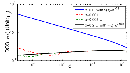
Figure 2: The TDOS for a finite long wire using Eq. (12) and the mode expansion Eq. (8). The parameters are: $L=10000$, $\alpha=0.01$, $g_{\rho}=0.5$, $g_{\sigma}=0.85$, $v_{\rho}=0.8$, $v_{\sigma}=0.47$, and $\rho_{0}=1/\sqrt{2\pi\alpha}$.

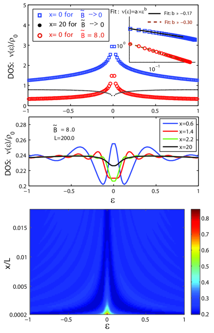
Figure 3: Upper panel: The blue square curve corresponds to $\widetilde{B}=\pi B/2\alpha\rightarrow 0$ and $x=0$ (we choose $\widetilde{B}=10^{-7}$ in numerics), with $\nu(\varepsilon)\propto\varepsilon^{-0.17}$, where the power exponent for the spinful LL is $g_{\rho}/2+1/(2g_{\sigma})-1=-0.162$. The black dotted curve is for $\widetilde{B}\rightarrow 0$ and $x=20.0$. The red circle curve is for $\widetilde{B}=8.0$ and $x=0$, with $\nu(\varepsilon)\propto\varepsilon^{-0.3}$. The inset shows the fitting to the power law expressions. Middle panel: TDOS at $x\neq 0$ from the SC-SLL interface. Lower panel: Two-dimensional map of the TDOS in the $x-\varepsilon$ plane. Parameters: $L=200.0$, $\alpha=0.04$, $g_{\rho}=0.5$, $g_{\sigma}=0.85$, $v_{\rho}=0.4$, $v_{\sigma}=0.235$, and $\chi=0$. The unit of TDOS is $L/2\pi$.

V Self-consistent harmonic approximation (SCHA)

The TDOS can be also obtained by using SCHA, i.e., expanding the cosine term in Eq. (4) up to the second order around one of the minima. Then, the effective Hamiltonian becomes quadratic

$$H_{\rm W}=\sum_{\nu=\rho,\sigma}\frac{v_{\nu}}{2}\int_{0}^{L}dx\big{[}g_{\nu}(\partial_{x}\theta_{\nu})^{2}+g^{-1}_{\nu}(\partial_{x}\phi_{\nu})^{2}\big{]}$$

$$\quad+\frac{\pi B}{2\alpha}\int_{0}^{L}dx\big{(}\phi_{\rho}+\theta_{\sigma}-(2l+1)\sqrt{\pi/2}\big{)}^{2}.$$ (17)

At this stage one inserts the mode expansion from Eq. (5) into Eq. (17), and diagonalizes the new Hamiltonian using the Bogolubov-Hopfield transformation numerically (see Appendix B). After the diagonalization, one can obtain the time evolution of the mode expansion in Eq. (5) in terms of their new eigenmodes and eigenenergies. The TDOS defined in Eqs. (9) and (10) can then be computed numerically.

In Fig. 3 we plot the resulting TDOS for a finite wire ($L=200$) at the Rashba wire-superconductor interface $x=0$ (upper panel) and at $x=0.6,1.4,2.2,20.0$ (lower panel) for $g_{\rho}=0.5$ and $g_{\sigma}=0.85$ as a function of the energy $\varepsilon$ (or equivalently bias voltage $eV$). The $B\rightarrow 0$ curve corresponds to the ordinary spinful Luttinger liquid, which shows zero-bias enhancement $\nu(\varepsilon)\propto\varepsilon^{g_{\rho}/2+1/(2g_{\sigma})-1}$ at the interfaces, which is consistent with Ref. Winkelholz96, . In contrast, farther away from the interface ($x=0.1L$), the TDOS displays the usual power law suppression at zero voltage bias. The curves for the nonvanishing field are shown for the case that $\mu$ lies in the the middle of the Zeeman gap $k_{F}=k_{\rm SO}$, i.e., SLL limit. At the interface the TDOS for the SLL also exhibits an anomalous enhancement at zero bias, but with a different power exponent [see Eq. (15)]. The middle panel shows the TDOS at $x=0.6,1.4,2.2,20.0$ away from the SC-SLL boundary. The zero-energy peak survives for small $x$ ($x=0.6$) and vanishes as $x$ increases. The TDOS for $x=0.6,1.4,2.2$ shows the oscillations and their amplitudes are reduced when increasing $x$. Those signatures are consistent with the factor $x^{-\eta/2-3\beta/2}$ in our analytical asymptotic result Eq. (16). Because of the suppression factor and the finite frequency resolution in numerics (note that there is always such a frequency cutoff in experiments), the oscillation disappears for large $x$ (e.g., $x=20.0$). A two-dimensional color map of the DOS near the SC-SLL interface $x=0$ as both functions of $\varepsilon$ and $x$ is plotted in the lower panel of Fig. 3, which shows the zero-bias enhancement near the SC-SLL interface, the zero-bias suppression far away from $x=0$, and the Friedel-type oscillation.

VI Summary

We have studied tunneling density of states into a quantum wire with strong spin-orbital coupling proximitized to superconductors. The delicate interplay of superconducting correlations and Luttinger liquid interactions leads to a dramatic change in the zero-bias anomaly which transforms into a peak. This signature is a consequence of the Andreev reflections at the SC-SLL interface. Our predictions may trigger new experiments and can be tested in carbon nanotubes Kasumov ; Morpurgo or InAs quantum wires. Vlad Perhaps it is plausible to argue that yet unexplained narrow needlelike resonance pinned at zero bias of a superconductor-InAs nanowire-superconductor device Vlad is in fact related to the anomalous enhancement of the density of states in a wire due to proximity effect and can be qualitative explained by our theory.

There is one important comment in order of the system under consideration. If the wire is built on top of a superconductor, the spiral Luttinger liquid, in the part that is proximitized to the superconducting bulk, is in its topological superconducting phase and thus supports Majorana fermions at the interfaces Gangadharaiah11 ; Sela11 ; Stoudenmire11 . In this case, the zero-bias anomaly peak feature due to Andreev reflections, discussed in this paper, coexists with the zero-bias peak due to the Majorana fermion law09 ; kouwenhovenSCI12 ; deng12 ; das12 . As the chemical potential is tuned far above the Zeeman gap the zero-bias anomaly peak due to Andreev reflection disappears, which also coincides with the disappearance of Majorana fermions. Therefore, our signature in the tunneling density of states masks the possible presence of the Majorana fermion. This brings yet another important detail that should be carefully looked at when interpreting experimental data.

Acknowledgments

D.E.L. was supported by Michigan State University and in part by ARO through Contract No. W911NF-12-1-0235. A.L. acknowledges support from NSF under Grant No. PHYS-1066293, and the hospitality of the Aspen Center for Physics where part of this work was performed.

Appendix A Derivation of TDOS in Eq. (15) and (16)

The TDOS is given in terms of the time correlation function

$$\nu(x,\varepsilon)=\!\!\int_{-\infty}^{+\infty}\!\!\frac{dt}{2\pi}\,e^{i\varepsilon t}\Big{[}\langle\Psi(x,t)\Psi^{\dagger}(x,0)\rangle+\langle\Psi^{\dagger}(x,0)\Psi(x,t)\rangle\Big{]},$$ (18)

where $\langle\Psi^{\dagger}(x,0)\Psi(x,t)\rangle$ can be computed similar to $\langle\Psi(x,t)\Psi^{\dagger}(x,0)\rangle$, and its result is obtained by changing $t$ to $-t$ in Eq. (14). At the SC-SLL interface $x=0$, the correlation function yields

$$\langle\Psi(0,t)\Psi^{\dagger}(0,0)\rangle=\frac{1}{\pi\alpha}\left[\frac{\alpha}{iu_{-}t+\alpha}\right]^{2\eta}.$$ (19)

Fourier transforming this one finds Eq. (15) of the main text.

For $x\neq 0$, the TDOS: $\nu(x,\varepsilon>0)$ can be obtained by integrating over $t$ along three branch cuts, i.e. $\mathbb{C}_{-1}$, $\mathbb{C}_{0}$, and $\mathbb{C}_{1}$ (with branching points $i\alpha$ and $\pm 2x/u_{-}+i\alpha$), with integrand $\langle\Psi(x,t)\Psi^{\dagger}(x,0)\rangle$ in the upper complex $t$ plane as shown in Fig. 4. The $\nu(x,\varepsilon<0)$ is obtained by integrating over $t$ along three other branch cuts with integrand $\langle\Psi^{\dagger}(x,0)\Psi(x,t)\rangle$ in the lower complex $t$ plane. Let us focus on the $\varepsilon>0$ case,

$$\nu(x,\varepsilon>0)=\frac{1}{2\pi^{2}\alpha}\int_{\mathbb{C}_{-1}+\mathbb{C}_{0}+\mathbb{C}_{1}}dte^{i\varepsilon t}\left[\frac{\alpha}{iu_{-}t+\alpha}\right]^{\eta+\beta}$$

$$\times\left[\frac{\alpha^{2}+(2x)^{2}}{[i(u_{-}t-2x)+\alpha][i(u_{-}t+2x)+\alpha]}\right]^{\frac{\eta-\beta}{2}}$$

$$=I_{\mathbb{C}_{-1}}+I_{\mathbb{C}_{0}}+I_{\mathbb{C}_{1}}.$$ (20)

In the limit $2x\varepsilon/u_{-}\gg 1$, the contribution of those branch cuts can be calculated independently. First of all, the integral $I_{\mathbb{C}_{0}}$ is

$$I_{\mathbb{C}_{0}}\approx\frac{1}{2\pi^{2}\alpha}\left[\frac{\alpha^{2}+(2x)^{2}}{(2x)^{2}}\right]^{\frac{\eta-\beta}{2}}\int_{\mathbb{C}_{0}}dte^{i\varepsilon t}\left[\frac{\alpha}{iu_{-}t}\right]^{\eta+\beta}$$

$$=\frac{1}{\pi\Gamma(\eta+\beta)u_{-}}\left[\frac{\alpha\varepsilon}{u_{-}}\right]^{\eta+\beta-1}$$ (21)

as $x\gg\alpha$. Second, the integral involving the path $I_{\mathbb{C}_{-1}}$ can be simplified by using a variable substitution $\tau=t+2x/u_{-}$,

$$I_{\mathbb{C}_{-1}}=\frac{1}{2\pi^{2}\alpha}\alpha^{\eta+\beta}(\alpha^{2}+4x^{2})^{\frac{\eta-\beta}{2}}e^{-i\frac{2x\varepsilon}{u_{-}}}$$

$$\times\!\!\int_{\mathbb{C}_{0}}\!\!\!d\tau e^{i\epsilon\tau}\!\!\left[\frac{1}{i(u_{-}\tau-2x)}\right]^{\eta+\beta}\!\!\left[\frac{1}{i(u_{-}\tau-4x)}\right]^{\frac{\eta-\beta}{2}}\!\!\left[\frac{1}{iu_{-}\tau}\right]^{\frac{\eta-\beta}{2}}$$

$$=\frac{\alpha^{\eta+\beta-1}i^{\frac{\eta-\beta}{2}}}{\pi\Gamma(\frac{\eta-\beta}{2})u_{-}}\left[\frac{i}{2}\right]^{\eta+\beta}\!\!\left[\frac{\varepsilon}{u_{-}}\right]^{\frac{\eta-\beta}{2}-1}\!\!\!x^{-\frac{\eta}{2}-\frac{3\beta}{2}}e^{-i\frac{2x\varepsilon}{u_{-}}}.$$ (22)

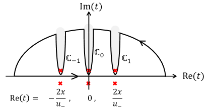
Figure 4: Integration contour in the upper complex plane of $t$. The red cross symbols are branching points for the correlation function $\langle\Psi(x,t)\Psi^{\dagger}(x,0)\rangle$ (upper plane) and $\langle\Psi^{\dagger}(x,0)\Psi(x,t)\rangle$ (lower plane).

Similarly, the last integral involving the path $I_{\mathbb{C}_{1}}$ can be simplified by using a variable substitution $\tau=t-2x/u_{-}$, and then

$$I_{\mathbb{C}_{1}}=\frac{\alpha^{\eta+\beta-1}(-i)^{\frac{\eta-\beta}{2}}}{\pi\Gamma(\frac{\eta-\beta}{2})u_{-}}\left[\frac{-i}{2}\right]^{\eta+\beta}\left[\frac{\varepsilon}{u_{-}}\right]^{\frac{\eta-\beta}{2}-1}\!\!\!x^{-\frac{\eta}{2}-\frac{3\beta}{2}}e^{i\frac{2x\varepsilon}{u_{-}}}.$$ (23)

Summing up all the terms, one can obtain the TDOS asymptote, i.e., Eq. (16) from the main text.

Appendix B Diagonalization of effective Hamiltonian in SCHA

Inserting the mode expansion from Eq. (5) into Eq. (17), we get

$$H = \frac{g_{\rho}v_{\rho}(J+\chi)^{2}}{4L}+\frac{v_{\sigma}M^{2}}{4Lg_{\sigma}}+\frac{\widetilde{B}L}{\pi}(\hat{\phi}_{\rho}^{0}+\hat{\theta}_{\sigma}^{0}-U_{min})^{2}$$ (24)

$$+\sum_{q>0}\Big{(}\sum_{\nu=\rho,\sigma}\frac{v_{\nu}}{2}q(2b_{\nu q}^{\dagger}b_{\nu q}+1)$$

$$+\frac{\widetilde{B}g_{\rho}}{2q}(b_{\rho q}^{\dagger}+b_{\rho q})^{2}+\frac{\widetilde{B}}{2g_{\sigma}q}(b_{\sigma q}^{\dagger}+b_{\sigma q})^{2}$$

$$+\frac{\widetilde{B}}{q}\sqrt{\frac{g_{\rho}}{g_{\sigma}}}(b_{\rho q}^{\dagger}+b_{\rho q})(b_{\sigma q}^{\dagger}+b_{\sigma q})\Big{)},$$

where $U_{min}=(2l+1)\sqrt{\pi/2}$. We can apply a canonical transformation to the topological part:

$$\Phi_{1} = \hat{\phi}_{\rho}^{0}+\hat{\theta}_{\sigma}^{0}-U_{min}\;,$$

$$N_{1} = [(J+\chi)+\kappa M]/(1+\kappa)\;,$$

$$\Phi_{2} = \sqrt{\kappa}\hat{\phi}_{\rho}^{0}-\hat{\theta}_{\sigma}^{0}/\sqrt{\kappa}\;,$$

$$N_{2} = \sqrt{\kappa}[(J+\chi)-M]/(1+\kappa)\;,$$ (25)

with $\kappa=v_{\sigma}/(v_{\rho}g_{\rho}g_{\sigma})$. By further introducing ladder operators $\eta_{1}$ and $\eta_{1}^{\dagger}$,

$$\Phi_{1}=\Xi^{-1/4}(\eta_{1}+\eta_{1}^{\dagger})/\sqrt{2}\;,$$

$$N_{1}=i\;\Xi^{1/4}(\eta_{1}^{\dagger}-\eta_{1})/\sqrt{2},$$ (26)

with $\Xi=4\widetilde{B}L^{2}/(\pi(g_{\rho}v_{\rho}+v_{\sigma}/g_{\sigma}))$, the topological part of Eq. (24) is reduced to

$$H_{\rm TOPO}=\sqrt{\frac{\widetilde{B}}{\pi}(g_{\rho}v_{\rho}+\frac{v_{\sigma}}{g_{\sigma}})}\Big{(}\eta_{1}^{\dagger}\eta_{1}-\frac{1}{2}\Big{)}+\frac{g_{\rho}v_{\rho}+\frac{v_{\sigma}}{g_{\sigma}}}{4L}N_{2}^{2}.$$ (27)

The non topological excitations can be diagonalized using the Bogolubov-Hopfield transformation, and we will briefly outline the main procedures below. This term can be diagonalized:

$$H_{\rm NT} = \sum_{q>0}\vec{b}_{q}\cdot H_{\mathrm{NT},q}\cdot\vec{b}_{q}^{T}$$ (28)

$$= \sum_{q>0}\vec{c}_{q}\cdot\rm{Diag}\{E_{1q},E_{2q},E_{1q},E_{2q}\}\cdot\vec{c}_{q}^{T}\;,\vspace{0.02in}$$

where $\vec{b}_{q}=(b_{\rho q}^{\dagger},b_{\sigma q}^{\dagger},b_{\rho q},b_{\sigma q})$ and the eigenvector after diagonalization is $\vec{c}_{q}=(c_{1q}^{\dagger},c_{2q}^{\dagger},c_{1q},c_{2q})$. The transformation matrix Q, i.e., $\vec{b}^{T}=\textbf{Q}\cdot\vec{c}^{T}$, can be obtained by the relation $\textbf{Q}=K\cdot M^{\dagger}\cdot K$, where $K=\rm{Diag}\{\mathbb{I}_{2\times 2},-\mathbb{I}_{2\times 2}\}$. The matrix $M^{\dagger}$ is obtained by solving the eigenvalue problem:

$$(H_{\mathrm{NT},q}K)M^{\dagger}=M^{\dagger}\rm{Diag}\{E_{1q},E_{2q},-E_{1q},-E_{2q}\}.$$ (29)

One can simply diagonalize the non topological part numerically. After the diagonalization, one can obtain the time evolution of the mode expansion for Eq. (5) of the main text in terms of their new eigenmode and eigenenergies. The TDOS is then computed numerically.

References

- (1) T. Giamarchi, Quantum Physics in One Dimension (Oxford University Press, 2004).
- (2) P. Strěda and P. Šeba, Phys. Rev. Lett. 90, 256601 (2003).
- (3) J. Sun, S. Gangadharaiah, and O. A. Starykh, Phys. Rev. Lett. 98, 126408 (2007); S. Gangadharaiah, J. Sun, and O. A. Starykh, Phys. Rev. B 78, 0554436 (2008).
- (4) B. Braunecker, P. Simon, and D. Loss, Phys. Rev. Lett. 102, 116403 (2009); Phys. Rev. B 80, 165119 (2009).
- (5) D. Schuricht, Phys. Rev. B 85, 121101(R) (2012).
- (6) B. Braunecker, C. Bena, and P. Simon, Phys. Rev. B 85, 035136 (2012).
- (7) C. P. Scheller, T.-M. Liu, G. Barak, A. Yacoby, L. N. Pfeiffer, K. W. West, D. M. Zumbühl, preprint arXiv:1306.1940.
- (8) T. Meng, L. Fritz, D. Schuricht, and D. Loss, preprint arXiv:1308.3169.
- (9) T. L. Schmidt, preprint arXiv:1306.6218.
- (10) R. M. Lutchyn, J. D. Sau, and S. Das Sarma, Phys. Rev. Lett. 105, 077001 (2010).
- (11) Y. Oreg, G. Refael, and F. von Oppen, Phys. Rev. Lett. 105, 177002 (2010).
- (12) V. Mourik, K. Zuo, S. M. Frolov, S. R. Plissard, E. P. A. M. Bakkers, and L. P. Kouwenhoven, Science 336 1003 (2012).
- (13) L. P. Rokhinson, X. Liu, and J. K. Furdyna, Nat. Phys. 8, 795 (2012).
- (14) M. T. Deng, C. L. Yu, G. Y. Huang, M. Larsson, P. Caroff, and H. Q. Xu, Nano Lett. 12, 6414 (2012).
- (15) A. Das, Y. Ronen, Y. Most, Y. Oreg, M. Heiblum, and H. Shtrikman, Nat. Phys. 8, 887 (2012).
- (16) S. Gangadharaiah, B. Braunecker, P. Simon, and D. Loss, Phys. Rev. Lett. 107, 036801 (2011).
- (17) E. Sela, A. Altland, and A. Rosch, Phys. Rev. B 84, 085114 (2011).
- (18) E. M. Stoudenmire, J. Alicea, O. A. Starykh, and M. P. A. Fisher Phys. Rev. B 84, 014503 (2011).
- (19) D. Esteve, H. Pothier, S. Gueron, and N. O. Birge, in Mesoscopic Electron Transport edited by L. L. Sohn (Kluwer 1997), pp. 375-406.
- (20) C. L. Kane and M. P. A. Fisher, Phys. Rev. Lett. 68, 1220 (1992).
- (21) C. Winkelholz, R. Fazio, F. W. J. Hekking, and G. Schön, Phys. Rev. Lett. 77, 3200 (1996).
- (22) D. L. Maslov, M. Stone, P. M. Goldbart, and D. Loss, Phys. Rev. B 53, 1548 (1996).
- (23) R. Fazio, F. W. J. Hekking, and A. A. Odintsov, Phys. Rev. Lett. 74, 1843 (1995); Phys. Rev. B 53, 6653 (1996).
- (24) S. Vishveshwara, C. Bena, L. Balents, and M. P. A. Fisher, Phys. Rev. B 66, 165411 (2002).
- (25) Y. Oreg and A. M. Finkelstein, Phys. Rev. Lett. 76, 4230 (1996).
- (26) L. Fidkowski, J. Alicea, N. H. Lindner, R. M. Lutchyn, and M. P. A. Fisher, Phys. Rev. B 85, 245121 (2012).
- (27) I. Ussishkin and L. I. Glazman, Phys. Rev. Lett. 93, 196403 (2004).
- (28) F. D. M. Haldane, J. Phys. C: Solid State Phys. 14, 2585 (1981); Phys. Rev. Lett. 47, 1840 (1981).
- (29) K. T. Law, P. A. Lee, and T. K. Ng, Phys. Rev. Lett. 103, 237001 (2009).
- (30) A. Yu. Kasumov, R. Deblock, M. Kociak, B. Reulet, H. Bouchiat, I. I. Khodos, Yu. B. Gorbatov, V. T. Volkov, C. Journet, M. Burghard, Science 284, 508 (1999).
- (31) A. F. Morpurgo, J. Kong, C. M. Marcus, H. Dai, Science 286, 263 (1999).
- (32) W. Chang, V. E. Manucharyan, T. S. Jespersen, J. Nygård, and C. M. Marcus, Phys. Rev. Lett. 110, 217005 (2013).