Charge transfer along DNA dimers, trimers and polymers

Abstract

The transfer of electrons and holes along DNA dimers, trimers and polymers is described at the base-pair level, using the relevant on-site energies of the base-pairs and the hopping parameters between successive base-pairs. The temporal and spatial evolution of carriers along a $N$ base-pair DNA segment is determined, solving a system of $N$ coupled differential equations. Useful physical quantities are calculated including the pure mean carrier transfer rate $k$, the inverse decay length $\beta$ used for exponential fit ($k=k_{0}\textrm{exp}(-\beta d)$) of the transfer rate as a function of the charge transfer distance $d=N\times$ 3.4 Å and the exponent $\eta$ used for a power law fit ($k=k_{0}^{\prime}N^{-\eta}$) of the transfer rate as function of the number of monomers $N$. Among others, the electron and hole transfer along the polymers poly(dG)-poly(dC), poly(dA)-poly(dT), GCGCGC…, ATATAT… is studied. $\beta$ ($\eta$) falls in the range $\approx$ 0.2 - 2 Å^-1 (1.7 - 17), $k_{0}$ ($k_{0}^{\prime}$) is usually $\approx 10^{-2}$-10^-1 ($10^{-2}$-10^-1) PHz although, generally, it falls in the wider range $\approx 10^{-4}$-10 ($10^{-4}$-10³) PHz. The results are compared with past predictions and experiments. Our approach illustrates to which extent a specific DNA segment can serve as an efficient medium for charge transfer.

Charge transfer along DNA is crucial for molecular biology, genetics, and nanotechnology GenereuxBarton:2010 ; Giese:2002 ; Endres:2004 . Here we present a convenient way to quantify electron or hole transfer along DNA segments using a tight-binding approach which can be easily implemented by interested colleagues. To date all the tight-binding parameters relevant to charge transport along DNA either for electrons (traveling through LUMOs) or for holes (traveling through HOMOs) are available in the literature  Endres:2004 ; HKS:2010-2011 ; Senthilkumar:2005 ; YanZhang:2002 ; SugiyamaSaito:1996 ; HutterClark:1996 ; ZhangLiEtAl:2002 ; LiCaiSevilla:2001 ; LiCaiSevilla:2002 ; ShuklaLeszczynski:2002 ; Varsano:2006 ; Voityuk:2001 ; Migliore:2009 ; Kubar:2008 ; Ivanova:2008 . Here we use them to study the temporal and spatial evolution of a carrier along DNA. The transport of electrons or holes can be described at either (I) the base-pair level or (II) the single base level HKS:2010-2011 . We need the relevant on-site energies of either (I) the base-pairs or (II) the single bases. In addition, we need the hopping parameters between either (I) successive base-pairs or (II) neighboring bases taking all possible combinations into account [(IIa) successive bases in the same strand, (IIb) complementary bases within a base-pair, (IIc) diagonally located bases of successive base-pairs in opposite strands]. To calculate the temporal and spatial evolution of carriers along a $N$ base-pair segment of DNA one has to solve a system of either (I) $N$ or (II) $2N$ coupled differential equations. Here we use the simplest approach (I) to examine charge transfer in B-DNA dimers, trimers and polymers. Taking the relevant literature into account Endres:2004 ; HKS:2010-2011 ; Senthilkumar:2005 ; YanZhang:2002 ; SugiyamaSaito:1996 ; HutterClark:1996 ; ZhangLiEtAl:2002 ; LiCaiSevilla:2001 ; LiCaiSevilla:2002 ; ShuklaLeszczynski:2002 ; Varsano:2006 ; Voityuk:2001 ; Migliore:2009 ; Kubar:2008 ; Ivanova:2008 , we use the on-site energies and the hopping parameters shown in Tables 1-2. We denote adenine (A), thymine (T), guanine (G), cytosine (C), and the relevant base-pairs A-T and G-C. YX signifies two successive base-pairs: the bases Y and X of two successive base-pairs (Y-Y${}_{\textrm{compl}}$ and X-X${}_{\textrm{compl}}$ separated and twisted by 3.4 Å and $36^{\circ}$) are located at the same strand in the direction $5^{\prime}-3^{\prime}$.

For a description at the base-pair level, the time-dependent single carrier (hole/electron) wave function of the DNA segment of interest, $\Psi^{DNA}_{H/L}({\bf r},t)$, is considered as a linear combination of base-pair wave functions with time-dependent coefficients, $\Psi^{DNA}_{H/L}({\bf r},t)=\sum_{\mu=1}^{N}A_{\mu}(t)\;\Psi^{bp(\mu)}_{H/L}({\bf r})$. $\Psi^{bp(\mu)}_{H/L}({\bf r})$ is the $\mu^{th}$ base-pair’s HOMO or LUMO wave function ($H/L$). The sum is extended over all base-pairs of the DNA segment under consideration. $|A_{\mu}(t)|^{2}$ gives the probability of finding the carrier at base-pair $\mu$, at time $t$. Starting from the time-dependent Schrödinger equation, $i\hbar\frac{\partial\Psi^{DNA}_{H/L}({\bf r},t)}{\partial t}=H^{DNA}\Psi^{DNA}_{H/L}({\bf r},t)$, following the procedure described in Ref. HKS:2010-2011 , we obtain that the time evolution of $A_{\mu}(t)$ obeys the tight-binding system of differential equations

$$i\hbar\frac{dA_{\mu}}{dt}=E^{bp(\mu)}_{H/L}A_{\mu}+t^{bp(\mu;\mu-1)}_{H/L}A_{\mu-1}+t^{bp(\mu;\mu+1)}_{H/L}A_{\mu+1}.$$ (1)

$E^{bp(\mu)}_{H/L}$ is the on-site energy of base-pair $\mu$, and $t^{bp(\mu;\mu^{\prime})}_{H/L}$ is the hopping parameter between base-pair $\mu$ and base-pair $\mu^{\prime}$. We can solve numerically the system of equations (1) and obtain, through $A_{\mu}(t)$, the time evolution of a carrier propagating along the DNA segment of interest.

Regarding the tight-binding description of hole transport, the corresponding tight-binding parameters should be taken with the opposite sign of the calculated on-site energies and transfer hopping integrals Senthilkumar:2005 . This means that for describing hole transport at the base-pair level, the on-site energies $E_{H}^{bp}$ presented in the second row of Table 1 and the hopping transfer integrals $t_{H}^{bp}$ presented in the second column of Table 2 should be used with opposite signs to provide the tight-binding parameters of Eq. 1. The on-site energies $E^{bp}_{H/L}$ for the two possible base-pairs A-T and G-C, calculated by various authors, are listed in Table 1. ${E^{bp\;\textrm{used}}_{H/L}}$ are the values actually used for the solution of Eq. 1 in this article. The hopping parameters $t_{H/L}^{bp}$ for all possible combinations of successive base-pairs, calculated by various authors, are given in Table 2. ${t^{bp\;\textrm{used}}_{H/L}}$ are the values actually used for the solution of Eq. 1 in this article. Due to the symmetry between base-pair dimers YX and X${}_{\textrm{compl}}$Y${}_{\textrm{compl}}$, the number of different hopping parameters is reduced from sixteen to ten. In Table 2 base-pair dimers exhibiting the same transfer parameters are listed together in the first column. We include in Table 2 the values listed: in Table 3 of Ref. HKS:2010-2011 , in Table II or Ref. Voityuk:2001 , in Table 5 (“Best Estimates”) of Ref. Migliore:2009 , in Table 4 of Ref. Kubar:2008 (two estimations given), in Table 2 of Ref. Ivanova:2008 , and the values extracted approximately from Fig. 4 of Ref. Endres:2004 . In Refs. Kubar:2008 ; Migliore:2009 ; Ivanova:2008 all values given are positive, in Ref. Voityuk:2001 the authors explicitly state that they quote absolute values, while in Refs. HKS:2010-2011 ; Endres:2004 the sign is included. In Ref. HKS:2010-2011 all $t_{H}^{bp}$ and $t_{L}^{bp}$ have been calculated, while in Ref. Endres:2004 only the values of $t_{H}^{bp}$ for a few cases are approximately given. According to Ref. BlancafortVoityuk:2006 the approximation used in Ref. Voityuk:2001 in general overestimates the transfer integrals. Summarizing, taking all the above into account, we use the values ${E^{bp\;\textrm{used}}_{H/L}}$ and ${t^{bp\;\textrm{used}}_{H/L}}$.

Table 1: The on-site energies $E^{bp}_{H/L}$ for the two possible base-pairs A-T and G-C, calculated by various authors. ${E^{bp\;\textrm{used}}_{H/L}}$ are the values actually used for the solution of Eq. 1 in this article. The first $\pi$-$\pi^{*}$ transition energies $E_{\pi-\pi^{*}}$ for the two B-DNA base-pairs are also shown. Except for Ref. HKS:2010-2011 these are ab initio calculations which tend to overestimate the first $\pi$-$\pi^{*}$ transition energy. All energies are given in eV.

B-DNA base-pair A-T G-C reference $E_{H}^{bp}$ $-$8.3 $-$8.0 HKS:2010-2011 $E_{L}^{bp}$ $-$4.9 $-$4.5 HKS:2010-2011 $E_{\pi-\pi^{*}}$ 3.4 3.5 HKS:2010-2011 $E_{H}^{bp\;\mathrm{first\;pr.}}$ $-$(7.8-8.2) $-$(6.3-7.7) SugiyamaSaito:1996 ; HutterClark:1996 ; ZhangLiEtAl:2002 ; LiCaiSevilla:2001 ; LiCaiSevilla:2002 ; ShuklaLeszczynski:2002 $E_{\pi-\pi^{*}}^{\mathrm{first\;pr.}}$ 6.4 4.3-6.3 ShuklaLeszczynski:2002 ; Varsano:2006 ${E^{bp\;\textrm{used}}_{H}}$ 8.3 8.0 HKS:2010-2011 ${E^{bp\;\textrm{used}}_{L}}$ $-$4.9 $-$4.5 HKS:2010-2011

Table 2: The hopping parameters between successive base-pairs for all possible combinations. $t_{H}^{bp}$ ($t_{L}^{bp}$) refers to hole (electron) hopping through HOMOs (LUMOs). The notation is given in the text. The values listed in Table 3 of Ref. HKS:2010-2011 , in Table II or Ref. Voityuk:2001 , in Table 5 (“Best Estimates”) of Ref. Migliore:2009 , in Table 4 of Ref. Kubar:2008 (two estimations given), in Table 2 of Ref. Ivanova:2008 , and the values extracted approximately from Fig. 4 of Ref. Endres:2004 are shown. These quantities represent the parameters $t^{bp(\mu;\mu\pm 1)}_{H/L}$ which appear in Eq. (1). Finally, ${t^{bp\;\textrm{used}}_{H/L}}$ are the parameters actually used in this work for the solution of Eq. 1. All hopping integrals $t_{H/L}^{bp}$ are given in meV.

Base-pair $t_{H}^{bp}$ $|t_{H}^{bp}|$ $t_{H}^{bp}$ $t_{H}^{bp}$ $t_{H}^{bp}$ $t_{H}^{bp}$ $t_{H}^{bp\;\textrm{used}}$ $t_{L}^{bp}$ $t_{L}^{bp}$ $t_{L}^{bp\;\textrm{used}}$ sequence HKS:2010-2011 Voityuk:2001 Endres:2004 Migliore:2009 Kubar:2008 Ivanova:2008 HKS:2010-2011 Endres:2004 AA, TT $-$8 26 $-$25 8-17 19(19) 22 20 $-$29 35 $-$29 AT 20 55 47(74) 37 $-$35 0.5 0.5 AG, CT $-$5 25 $-$50 35(51) 43 30 3 35 3 AC, GT 2 26 25(38) 20 $-$10 32 32 TA 47 50 32(68) 52 $-$50 2 2 TG, CA $-$4 27 11(11) 25 10 17 17 TC, GA $-$79 122 $-$160 71(108) 60 110 $-$1 35 $-$1 GG, CC $-$62 93 $-$140 75 72(101) 63 100 20 35 20 GC 1 22 20(32) 22 $-$10 $-$10 $-$10 CG $-$44 78 51(84) 74 50 $-$8 $-$8

We define the column vector matrix $\vec{x}(t)$ made from $A_{j}(t),\;j=1,\dots,N$. Hence, $\dot{\vec{x}}(t)=\widetilde{\mathcal{A}}\vec{x}(t)$, $\widetilde{\mathcal{A}}=-\frac{i}{\hbar}\textrm{A}$. A is a symmetric tridiagonal matrix. To proceed, we use the eigenvalue method, i.e. we look for solutions of the form $\vec{x}(t)=\vec{v}e^{\tilde{\lambda}t}\Rightarrow\dot{\vec{x}}(t)=\tilde{\lambda}\vec{v}e^{\tilde{\lambda}t}$. $\widetilde{\mathcal{A}}\vec{v}=\tilde{\lambda}\vec{v}$, or $\textrm{A}\vec{v}=\lambda\vec{v}$, with $\tilde{\lambda}=-\frac{i}{\hbar}\lambda$. Having checked that the normalized eigenvectors $\vec{v_{k}}$ corresponding to the eigenvalues $\lambda_{k}$ are linearly independent, the solution is $\vec{x}(t)=\sum_{k=1}^{N}c_{k}\vec{v_{k}}e^{-\frac{i}{\hbar}\lambda_{k}t}$. From the initial conditions we determine $c_{i}(t)$.

For dimers, supposing that $\lambda_{2}\geq\lambda_{1}$, we obtain the period of $|A_{\mu}(t)|^{2},\mu=1,2$, $T=\frac{h}{\lambda_{2}-\lambda_{1}}$. For a dimer consisting of two identical monomers with purine on purine (GG $\equiv$ CC, AA $\equiv$ TT), $\lambda_{1,2}=E^{bp}\mp t^{bp}$. Then, if we initially place the carrier in monomer 1, $|A_{1}(t)|^{2}=\frac{1}{2}+\frac{1}{2}\textrm{cos}[\frac{(\lambda_{2}-\lambda_{1})t}{\hbar}]$, $|A_{2}(t)|^{2}=\frac{1}{2}-\frac{1}{2}\textrm{cos}[\frac{(\lambda_{2}-\lambda_{1})t}{\hbar}]$. For a dimer consisting of two identical monomers with purine on pyrimidine (GC, CG, AT, TA), the problem is identical. For a dimer made up of different monomers (AG ​​​ $\equiv$ ​​​ CT, AC ​​​ $\equiv$ ​​​ GT, TG ​​​ $\equiv$ ​​​ CA, TC ​​​ $\equiv$ ​​​ GA), $\lambda_{1,2}=\frac{E^{bp1}+E^{bp2}}{2}\mp\sqrt{\frac{(E^{bp1}-E^{bp2})^{2}}{4}+{t^{bp}}^{2}}$. Hence, for identical monomers $T\!\!=\!\!\frac{h}{2|t^{bp}|}$, for different monomers, $T=\frac{h}{\sqrt{(2t^{bp})^{2}+(\Delta^{bp})^{2}}}$. $\Delta^{bp}=|E^{bp1}-E^{bp2}|$. The maximum transfer percentage of the carrier from base-pair 1 to base-pair 2, $p=4c_{1}v_{11}c_{2}v_{12}$. This refers to the maximum of $|A_{2}(t)|^{2}$. $v_{ij}$ is the $i$-th component of eigenvector $j$. Hence, $p=\frac{(2t^{bp})^{2}}{(2t^{bp})^{2}+(\Delta^{bp})^{2}}$. For identical (different) monomers, $p=1$ ($p<1$). The pure maximum transfer rate can be defined as $\frac{p}{T}=\frac{(2t^{bp})^{2}}{h\sqrt{(2t^{bp})^{2}+(\Delta^{bp})^{2}}}$. For identical monomers, $\frac{p}{T}=\frac{2|t^{bp}|}{h}$. For holes, when purines are crosswise to pyrimidines (GT $\equiv$ AC, CA $\equiv$ TG) $p$ is negligible, hence, we expect that insertion of these dimers in a sequence of DNA base-pairs will disrupt hole transfer. Also AG $\equiv$ CT has very small $p$. Generally, electrons have smaller $p$ than holes. In contrast to the cases of holes, when purines are NOT crosswise to pyrimidines (GA $\equiv$ TC, CT $\equiv$ AG) $p$ is negligible, hence, we expect that insertion of these dimers in a sequence of DNA base-pairs will disrupt electron transfer. Generally, in cases of different monomers $T$ is smaller than in cases of identical monomers due to the extra term containing $\Delta^{bp}=|E^{bp1}-E^{bp2}|$. Overall, carrier transfer is more difficult for different monomers compared to identical monomers. If $|A_{2}(0)|^{2}=0$, a pure mean transfer rate can be defined as $k=\frac{\langle|A_{2}(t)|^{2}\rangle}{{t_{2}}_{mean}}$, where ${t_{2}}_{mean}$ is the first time $|A_{2}(t)|^{2}$ becomes equal to $\langle|A_{2}(t)|^{2}\rangle$ i.e. “the mean transfer time”. Figure 1 shows $T$, $p$, $p/T$ and $k=\langle|A_{2}(t)|^{2}\rangle/{t_{2}}_{mean}$.

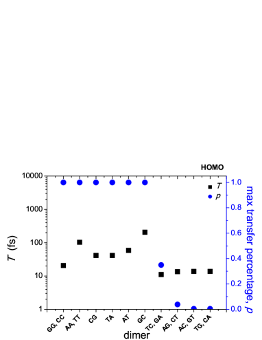
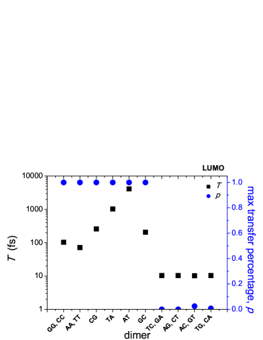
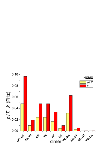
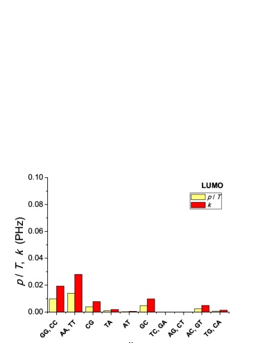
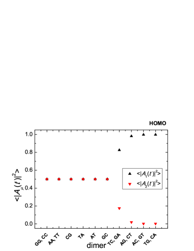
Figure 1: Dimers: the period of carrier transfer between monomers $T$ (fs) and the maximum transfer percentage $p$ [1st row], the pure maximum transfer rate defined as $p/T$ (PHz) and the pure mean transfer rate defined as $k=\langle|A_{2}(t)|^{2}\rangle/{t_{2}}_{mean}$ (PHz) [2nd row]. $\langle|A_{\mu}(t)|^{2}\rangle,\;\mu=1,2$, which describe the spread of the carrier over the monomers constituting the dimer [3rd row]. For the dimers made up of identical monomers $p=1$ whereas for the dimers made up of different monomers $p<1$. In the latter case, the pure maximum transfer rate and the pure mean transfer rate are negligible for HOMO hole transfer when purines are crosswise to pyrimidines (GT $\equiv$ AC and CA $\equiv$ TG dimers) and for LUMO electron transfer when purines are on top of pyrimidines (GA $\equiv$ TC and CT $\equiv$ AG dimers). For dimers $k=2\frac{p}{T}$.

For trimers, supposing that $\lambda_{1}\leq\lambda_{2}\leq\lambda_{3}$, we conclude that $|A_{\mu}(t)|^{2},\mu=1,2,3$ are sums of terms containing constants and periodic functions with periods $T_{21}=\frac{h}{\lambda_{2}-\lambda_{1}},T_{32}=\frac{h}{\lambda_{3}-\lambda_{2}},T_{31}=\frac{h}{\lambda_{3}-\lambda_{1}}$. There are 8 trimers consisting of identical monomers. In the cases of 0 times crosswise purines $\lambda_{2}=E^{bp},\lambda_{1,3}=E^{bp}\mp t^{bp}\sqrt{2}$. Hence, two periods are involved in $|A_{\mu}(t)|^{2},\mu=1,2,3$: $T_{M}=\frac{h}{t^{bp}\sqrt{2}},T_{E}=\frac{h}{2t^{bp}\sqrt{2}}\Rightarrow\;\;\frac{T_{M}}{T_{E}}=\frac{2}{1}$. $T_{M}=T_{M(21)}=T_{M(32)}$ involves the Medium eigenvalue, $T_{E}=T_{E(31)}$ involves only the Edge eigenvalues. Since $\frac{T_{M}}{T_{E}}=\frac{2}{1}$, $|A_{\mu}(t)|^{2},\mu=1,2,3$ are periodic. In the cases of 1 or 2 times crosswise purines $\lambda_{2}=E^{bp},\lambda_{1,3}=E^{bp}\mp\sqrt{{t^{bp}}^{2}+{t^{bp^{\prime}}}^{2}}$. Hence, two periods are involved in $|A_{\mu}(t)|^{2},\mu=1,2,3$: $T_{M}=\frac{h}{\sqrt{{t^{bp}}^{2}+{t^{bp^{\prime}}}^{2}}},T_{E}=\frac{h}{2\sqrt{{t^{bp}}^{2}+{t^{bp^{\prime}}}^{2}}}\Rightarrow\frac{T_{M}}{T_{E}}=\frac{2}{1}$. Since $\frac{T_{M}}{T_{E}}=\frac{2}{1}$ it follows that $|A_{\mu}(t)|^{2},\mu=1,2,3$ are periodic. Conclusively, in all cases of a trimer consisting of identical monomers, $|A_{\mu}(t)|^{2},\mu=1,2,3$ are periodic with period $T_{M}$. Suppose that we have a trimer consisting of different monomers. There are 24 different such trimers. For example, suppose that we refer to HOMO charge transfer in GAC $\equiv$ GTC, then with $E^{bp^{\prime\prime}}>E^{bp}$, $\lambda_{2}=E^{bp},\lambda_{1,3}\!=\!\frac{E^{bp}+E^{bp^{\prime\prime}}}{2}\!\mp\!\sqrt{\left(\frac{E^{bp}-E^{bp^{\prime\prime}}}{2}\right)^{2}\!+\!{t^{bp}}^{2}+{t^{bp^{\prime}}}^{2}}$. Three periods are involved in $|A_{\mu}(t)|^{2},\mu=1,2,3$. With $\Delta^{bp}=|E^{bp}-E^{bp^{\prime\prime}}|$, $T_{M(32)}=\frac{h}{\frac{\Delta^{bp}}{2}+\sqrt{\frac{{\Delta^{bp}}^{2}}{4}+{t^{bp}}^{2}+{t^{bp^{\prime}}}^{2}}},T_{E(31)}=\frac{h}{2\sqrt{\frac{{\Delta^{bp}}^{2}}{4}+{t^{bp}}^{2}+{t^{bp^{\prime}}}^{2}}},T_{M(21)}=\frac{h}{-\frac{\Delta^{bp}}{2}+\sqrt{\frac{{\Delta^{bp}}^{2}}{4}+{t^{bp}}^{2}+{t^{bp^{\prime}}}^{2}}}.$ $\frac{T_{M(32)}}{T_{E(31)}}$ and $\frac{T_{M(21)}}{T_{E(31)}}$ may be irrational numbers, hence $|A_{\mu}(t)|^{2},\mu=1,2,3$ may be non-periodic.

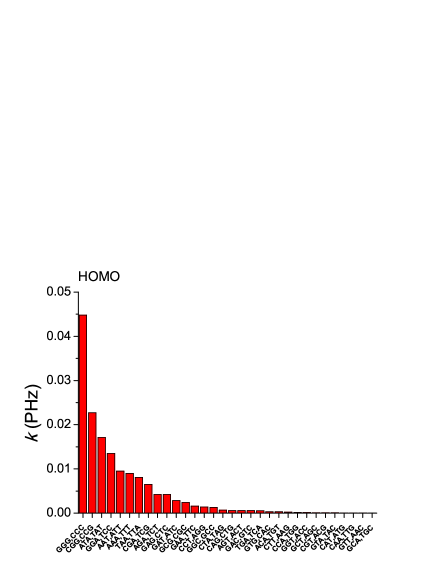
Figure 2: HOMO pure mean transfer rate $k$ for all trimers.

Since for trimers consisting of different monomers $|A_{\mu}(t)|^{2},\mu=1,2,3$ may be non-periodic, from now on we will only use the pure mean transfer rate $k$, which if $|A_{3}(0)|^{2}=0$, can be defined as $k=\frac{\langle|A_{3}(t)|^{2}\rangle}{{t_{3}}_{mean}}$, where ${t_{3}}_{mean}$ is the first time $|A_{3}(t)|^{2}$ becomes equal to $\langle|A_{3}(t)|^{2}\rangle$ i.e. “the mean transfer time”. The HOMO pure mean transfer rate $k$ for all possible trimers is shown in Fig. 2. For trimers consisting of identical monomers $k\approx 1.3109\frac{p}{T}$. As expected, $k$ is very small when trimers include dimers with very small $k$, primarily purines crossswise to pyrimidines (GT ​​​ $\equiv$ ​​​ AC, CA ​​​ $\equiv$ ​​​ TG), secondarily AG ​​​ $\equiv$ ​​​ CT, thirdly GC.

For polymers, supposing that $|A_{N}(0)|^{2}=0$, for a polymer consisting of $N$ monomers, a pure mean transfer rate can be defined as $k=\frac{\langle|A_{N}(t)|^{2}\rangle}{{t_{N}}_{mean}}$, where ${t_{N}}_{mean}$ is the first time $|A_{N}(t)|^{2}$ becomes equal to $\langle|A_{N}(t)|^{2}\rangle$ i.e. “the mean transfer time”. Increasing the number of base-pairs or monomers $N$, we study various characteristic polymers: poly(dG)-poly(dC), poly(dA)-poly(dT), GCGCGC…, CGCGCG…, ATATAT…, TATATA… as well as DNA segments that have been experimentally studied in the past. If we fit $k(d)$ –i.e. the pure mean transfer rate $k$ as a function of the charge transfer distance $d=N\times$ 3.4 Å– exponentially, as $k=k_{0}\textrm{exp}(-\beta d)$, we obtain an estimation of $k_{0}$ and of the distance dependence parameter or inverse decay length $\beta$ Marcus . These quantities are displayed in Table 3. If, instead, we fit $k(N)$ –i.e. the pure mean transfer rate $k$ as a function of the number of monomers $N$– in a power law, as $k=k_{0}^{\prime}N^{-\eta}$, we obtain an estimation of $k_{0}^{\prime}$ and $\eta$. These quantities are displayed in Table 4. Values of $\beta$, in the range $\approx$ 0.3-1.5 Å^-1, for various compounds, have been displayed in the literature at least 30 years now, see e.g Table IV of Ref. Marcus . In Table 3 the values of $\beta$ are in the range $\approx$ 0.2-2 Å^-1, with smaller values for periodic polymers like ATATAT…, poly(dG)-poly(dC), poly(dA)-poly(dT). However, for efficient charge transfer, a small value of $\beta$ is not enough; one should also take into account the magnitude of $k_{0}$. The values of $k_{0}$ assumed in Ref. Marcus are 10^-2-10^-1 PHz which coincides with most of the $k_{0}$ values shown in Table 3, although generally, the values of $k_{0}$ fall in the wider range $\approx 10^{-4}$-10 PHz. For the power law fit, $\eta\approx$ 1.7 - 17; most of the $k_{0}^{\prime}$ values shown in Table 4 are in the range $\approx 10^{-2}$-10^-1 PHz, although generally, the values of $k_{0}^{\prime}$ fall in the wider range $\approx 10^{-4}$-10³ PHz. The $\beta$-value for charge transfer from an initial site (donor) to a final site (acceptor) depends on the mediating molecules, the so-called bridge. From Table 3 we conclude that there are no universal values of $\beta$ and $k_{0}$ for DNA, instead, each specific DNA segment is unique and one should use an efficient and easy way to predict $\beta$ and $k_{0}$ of each DNA segment under investigation. It is hoped that the present work will contribute in this direction. $\beta$ values for different systems include $\approx$ 1.0 - 1.4 Å^-1 for protein-bridged systems  Moser:1992 ; GrayWinkler:2005 , $\approx$ 1.55 - 1.65 Å^-1 for aqueous glass bridges GrayWinkler:2005 , $\approx$ 0.2 - 1.4 Å^-1 for DNA segments Lewis:1997 ; Holmlin:1998 ; Henderson:1999 ; Wan:2000 ; KawaiMajima:2013 ; KalosakasSpanou:2013 , $\approx$ 0.8 - 1.0 Å^-1 for saturated hydrocarbon bridges Johnson:1989 ; Oevering:1987 , $\approx$ 0.2 - 0.6 Å^-1 for unsaturated phenylene Helms:1992 ; Ribou:1994 , polyene Effenberger:1991 ; Tolbert:1992 and polyyne Grosshenny:1996 ; Sachs:1997 bridges, and much smaller values ($<$ 0.05 Å^-1), suggesting a molecular-wire-like behavior, for a p-phenylenevinylene bridge Davis:1998 . Hence, it seems that charge transfer in ATATAT…, poly(dG)-poly(dC) and poly(dA)-poly(dT) is almost molecular-wire-like. Since a carrier can migrate along DNA over 200 Å Meggers:1998 ; Henderson:1999 ; KawaiMajima:2013 , in the present calculations for polymers $d$ is extending up to 204 Å ($N$ up to 60 base-pairs).

Table 3: $k_{0}$ and $\beta$ of the exponential fit $k=k_{0}\textrm{exp}(-\beta d)$ for various DNA polymers. C.C. is the correlation coefficient.

DNA segment	$k_{0}$ (PHz)	$\beta$ (Å-1)	C.C.	H/L
poly(dG)-poly(dC)	0.176 $\pm$ 0.007	0.189 $\pm$ 0.008	0.988	H
poly(dG)-poly(dC)	0.035 $\pm$ 0.001	0.189 $\pm$ 0.007	0.989	L
poly(dA)-poly(dT)	0.035 $\pm$ 0.001	0.189 $\pm$ 0.008	0.988	H
poly(dA)-poly(dT)	0.051 $\pm$ 0.002	0.189 $\pm$ 0.008	0.989	L
GCGCGC…	0.032 $\pm$ 0.003	0.358 $\pm$ 0.023	0.988	H
ATATAT…	0.057 $\pm$ 0.002	0.168 $\pm$ 0.008	0.985	H
CGCGCG…	0.932 $\pm$ 0.233	0.871 $\pm$ 0.074	0.994	H
TATATA…	0.110 $\pm$ 0.005	0.251 $\pm$ 0.012	0.985	H
AGTGCCAAGCTTGCA	0.059 $\pm$ 0.002	0.685 $\pm$ 0.008	1.000	H
AGTGCCAAGCTTGCA	$(9.8\!\pm\!2.6)\!\!\times\!\!10^{-5}$	0.197 $\pm$ 0.059	0.808	L
TAGAGGTGTTATGA	4.306 $\pm$ 5.001	1.321 $\pm$ 0.342	0.998	H
TAGAGGTGTTATGA	2.877 $\pm$ 0.833	2.154 $\pm$ 0.085	1.000	L

Table 4: $k_{0}^{\prime}$ and $\eta$ of the power fit $k=k_{0}^{\prime}N^{-\eta}$ for various DNA polymers. C.C. is the correlation coefficient.

DNA segment	$k_{0}^{\prime}$ (PHz)	$\eta$	C.C.	H/L
poly(dG)-poly(dC)	0.359 $\pm$ 0.001	1.893 $\pm$ 0.002	1.000	H
poly(dG)-poly(dC)	0.072 $\pm$ 0.000	1.895 $\pm$ 0.002	1.000	L
poly(dA)-poly(dT)	0.072 $\pm$ 0.000	1.892 $\pm$ 0.002	1.000	H
poly(dA)-poly(dT)	0.105 $\pm$ 0.000	1.893 $\pm$ 0.002	1.000	L
GCGCGC…	0.087 $\pm$ 0.008	3.176 $\pm$ 0.127	0.993	H
ATATAT…	0.117 $\pm$ 0.004	1.776 $\pm$ 0.035	0.994	H
CGCGCG…	5.082 $\pm$ 1.619	6.715 $\pm$ 0.458	0.994	H
TATATA…	0.236 $\pm$ 0.007	2.295 $\pm$ 0.035	0.997	H
AGTGCCAAGCTTGCA	1.383 $\pm$ 0.826	4.487 $\pm$ 0.487	0.997	H
AGTGCCAAGCTTGCA	$(2.2\!\pm\!1.0)\!\!\times\!\!10^{-4}$	2.176 $\pm$ 0.543	0.761	L
TAGAGGTGTTATGA	46.300 $\pm$53.288	9.902 $\pm$ 1.660	0.998	H
TAGAGGTGTTATGA	203.457$\pm$99.552	16.708 $\pm$ 0.706	1.000	L

In Ref. WangLewisSankey:2004 the authors calculated the complex band structure of poly(dA)-poly(dT) and poly(dG)-poly(dC) using an ab initio tight-binding method based on density-functional theory and obtained the energy dependence $\beta(E)$. Since the states with large $\beta$ values don’t play a significant role in conduction they noticed that only the smallest $\beta(E)$ states, described by a semielliptical-like curve in the band-gap region are important. This branch reaches a maximum $\beta$ value near midgap, called the branch point, $\beta_{bp}$, $\approx$ 1.5 Å^-1 both for poly(dA)-poly(dT) and poly(dG)-poly(dC). Since in molecular electronics metallic contacts are made at the two ends of the molecule and electronic current is carried by electrons tunneling from the metal with energies in the band-gap region, the branch point plays an important role in the conductance. Although the above hold when metal conducts are attached to the molecule, in photoinduced charge transfer experiments, we are interested in states close to the top of the valence band i.e. the HOMO or close to the bottom of the conduction band i.e. the LUMO. For the top of the valence band of poly(dA)-poly(dT) [Fig.1a of Ref. WangLewisSankey:2004 ] $\beta\approx$ 0.4 Å^-1 and for poly(dG)-poly(dC) [Fig.1b of Ref. WangLewisSankey:2004 ] $\beta\approx$ 0.2 Å^-1, close to the values predicted in the present work ($\approx$ 0.2 Å^-1 both for poly(dA)-poly(dT) and poly(dG)-poly(dC) cf. Table 3).

In Ref. Giese:2001 Giese et al. studied experimentally the hole transfer in the DNA segment [G] (T)n [GGG] TATTATATTACGC. (T)n denotes the bridge made up from $n$ T-A monomers between the hole donor [G] and the hole acceptor [GGG] denoted by square brackets, before the TATTATATTACGC tail. In Fig. 3 the computed $k(d)$ i.e. the pure mean transfer rate as a function of the distance from the hole donor to the middle of the hole acceptor is shown. In accordance with the experiment Giese:2001 we find two regions with different distance dependence. For $n=1,2,3$ the distance dependence is strong becoming much weaker for $n\geq 4$. For the strong distance dependence range, we find $\beta\approx$ 0.8 Å^-1. In the experiment [Fig. 3 of Ref. Giese:2001 ] the authors find qualitatively the same behavior, estimating $\beta\approx$ 0.6 Å^-1 for $n=1,2,3$. For $n=4,\dots,16$ we compute a much weaker distance dependence with $\beta\approx$ 0.07 Å^-1.

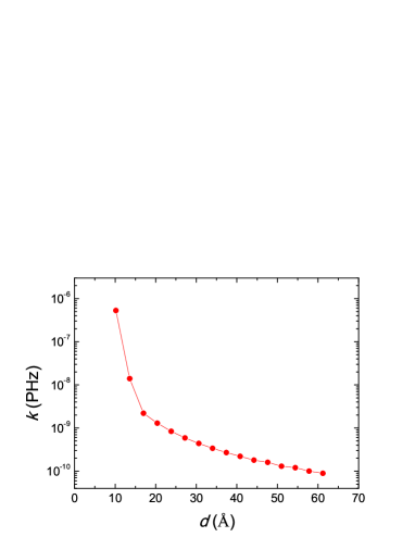
Figure 3: Experiment of Giese et al. Giese:2001 , i.e. [G] (T)n [GGG] TATTATATTACGC. (T)n denotes the bridge made up from $n$ T-A monomers between the hole donor G (the first G-C monomer) and the hole acceptor GGG (the trimer made by three G-C monomers) before the TATTATATTACGC tail. the hole donor and acceptor denoted by square brackets. For the strong distance dependence $k(d)$ range (for $n=$ 1,2,3), $\beta\approx$ 0.8 Å^-1. In the experiment [Figure 3 of Ref. Giese:2001 ] the authors find qualitatively the same behavior, while they estimate $\beta\approx$ 0.6 Å^-1 (for $n=1,2,3$) i.e. for the strong distance dependence range. For the weak distance dependence region, again in agreement with the experiment, a much weaker distance dependence with $\beta\approx$ 0.07 Å^-1 is obtained.

In Ref. Murphy:1993 the authors demonstrated rapid photoinduced electron transfer over a distance of greater than 40 Å between metallointercalators tethered to the 5^′ termini of AGTGCCAAGCTTGCA. The authors Murphy:1993 mentioned that “the photoinduced electron transfer between intercalators occurs very rapidly over $>$ 40 Å through the DNA helix over a pathway consisting of $\pi$-stacked base-pairs.” Then, from Marcus theory Marcus they estimated $\beta$ to be $\leq$ 0.2 Å^-1. We observe (Table 3) that for electron transfer (through LUMOs) we also find $\beta\leq$ 0.2 Å^-1, while for hole transfer (through HOMOs) we find $\beta\approx$ 0.7 Å^-1. Similar weak distance dependence with $\beta\leq$ 0.2 Å^-1 was found in Ref. Arkin:1996 .

In Ref. Giese:1999 the authors study hole transfer in the DNA sequence ACGCACGTCGCATAATATTACG [bridge] GGGTATTATATTACGC, where the [bridge] is either TT (sample 1a, one TT step) either TTGTT (sample 2a, two TT steps) or TTGTTGTTGTT (sample 3a, four TT steps). The hole is created in the C-G monomer before the G-C monomer before the [bridge] and transferred to the GGG trimer. The charge transfer is measured by “the oxidative damage at the G and GGG units”, “quantified after piperidine treatment and polyacrylamide gel electrophoresis with a phospho-imager”. To compare our results with the experiment we need the ratio of $\sum_{j}\langle|A_{j}(t)|^{2}\rangle$ where $j$ represents the three monomers of the GGG trimer to $\langle|A_{i}(t)|^{2}\rangle$ where $i$ represents the initial G-C monomer (called also G₂₃). This ratio is called GGGperG23 in Fig. 4. Our calculations with three or four TT steps confirm the experiment either using an exponential fit with the $\beta$ parameter or a power law fit with the $\eta$ parameter. Extending the present approach up to eight TT steps reveals (Fig. 4) that there are two distinct regions (i) one step (S1) to two steps (S2), and (ii) more than two steps (up to eight steps are included in the graphs).

Figure 4: Hole transfer in ACGCACGTCGCATAATATTACG [bridge] GGGTATTATATTACGC. The [bridge] is made up of TT dimers separated by G monomers. In the experiment Giese:1999 , [bridge] is either TT (one TT step) either TTGTT (two TT steps) or TTGTTGTTGTT (four TT steps).

A handy method to examine the charge transfer properties of DNA segments was displayed. Useful physical quantities were obtained including the pure mean carrier transfer rate $k$, the inverse decay length $\beta$ used for an exponential fit ($k=k_{0}\textrm{exp}(-\beta d)$) of the transfer rate as a function of the charge transfer distance $d=N\times$ 3.4 Å and the exponent $\eta$ used for a power law fit ($k=k_{0}^{\prime}N^{-\eta}$) of the transfer rate as function of the number of monomers $N$. The values of these parameters are not universal, depend on the specific DNA segment and are different for electrons and holes.

References

- (1) J.C. Genereux and J.K. Barton, Chem. Rev. 110, 1642 (2010).
- (2) B. Giese, Annu. Rev. Biochem. 71, 51 (2002).
- (3) R.G. Endres, D.L. Cox, and R.R.P. Singh, Rev. Mod. Phys. 76, 195 (2004).
- (4) L.G.D. Hawke, G. Kalosakas, and C. Simserides, Eur. Phys. J. E 32, 291 (2010); ibid. 34, 118, (2011).
- (5) K. Senthilkumar, F.C. Grozema, C.F. Guerra, et al., J. Am. Chem. Soc. 127, 14894 (2005).
- (6) Y. J. Yan and H. Zhang, J. Theor. Comput. Chem. 1, 225 (2002).
- (7) H. Sugiyama and I. Saito, J. Am. Chem. Soc. 118, 7063 (1996).
- (8) M. Hutter and T. Clark, J. Am. Chem. Soc. 118, 7574 (1996).
- (9) H. Zhang, X.Q. Li, P. Ham, X.Y. Yu, and Y.J. Yan, J. Chem. Phys. 117, 4578 (2002).
- (10) X. Li, Z. Cai, and M.D. Sevilla, J. Phys. Chem. B 105, 10115 (2001).
- (11) X. Li, Z. Cai, and M.D. Sevilla, J. Phys. Chem. A 106, 9345 (2002).
- (12) M. K. Shukla and J. Leszczynski, J. Phys. Chem. A 106, 4709 (2002).
- (13) D. Varsano, R. Di Felice, M. A. L. Marques, and A. Rubio, J. Phys. Chem. B 110, 7129 (2006).
- (14) A. A. Voityuk, J. Jortner, M. Bixon, and N. Rösch, J. Chem. Phys. 114, 5614 (2001).
- (15) A. Migliore, S. Corni, D. Varsano, M.L. Klein, and R. Di Felice, J. Phys. Chem. B 113, 9402 (2009).
- (16) T. Kubař, P. B. Woiczikowski, G. Cuniberti, and M. Elstner, J. Phys. Chem. B 112, 7937 (2008).
- (17) A. Ivanova, P. Shushkov, and N. Rösch, J. Phys. Chem. A 112, 7106 (2008).
- (18) L. G. D. Hawke, G. Kalosakas, and C. Simserides, Mol. Phys. 107, 1755 (2009).
- (19) L. Blancafort and A. A. Voityuk, J. Phys. Chem. A 110, 6426 (2006).
- (20) R.A. Marcus and N. Sutin, Biochim. Biophys. Acta 811, 265 (1985) and references therein.
- (21) H.B. Gray and J.R. Winkler, Proc. Natl. Acad. Sci. U.S.A. 102 (2005) 3534.
- (22) C.C. Moser, J.M. Keske, K. Warncke, R.S. Farid, P.L. Dutton, Nature 355, 796 (1992).
- (23) K. Kawai and T. Majima, Acc. Chem. Res., Publication Date (Web): June 27, 2013, DOI: 10.1021/ar400079s
- (24) F.D. Lewis, T. Wu, Y. Zhang, R.L. Letsinger, S.R. Greenfield, M.R. Wasielewski, Science 277, 673 (1997).
- (25) C.Z. Wan, T. Fiebig, O. Schiemann, J.K. Barton, A.H. Zewail, Proc. Natl. Acad. Sci. U.S.A. 97, 14052 (2000).
- (26) R.E. Holmlin, P.J. Dandliker, J.K. Barton, Angew. Chem. Int. Edn. Engl. 36, 2715 (1998).
- (27) P.T. Henderson, D. Jones, G. Hampikian, et al., Proc. Natl. Acad. Sci. USA 96, 8353 (1999).
- (28) G. Kalosakas and E. Spanou, Phys. Chem. Chem. Phys. 15, 15339 (2013).
- (29) M.D. Johnson, J.R. Miller, N.S. Green, G.L. Closs, J. Phys. Chem. 93, 1173 (1989).
- (30) H. Oevering, M.N. Paddon-Row, M. Heppener, et al., J. Am. Chem. Soc. 109, 3258 (1987).
- (31) A. Helms, D. Heiler, G. McLendon, J. Am. Chem. Soc. 114, 6227 (1992).
- (32) A.-C. Ribou, J.-P. Launay, K. Takahashi, T. Nihira, S. Tarutani, C.W. Spangler, Inorg. Chem. 33, 1325 (1994).
- (33) F. Effenberger and H.C. Wolf, New J. Chem. 15, 117 (1991).
- (34) L.M. Tolbert, Acc. Chem. Res. 25, 561 (1992).
- (35) V. Grosshenny, A. Harriman, R. Ziessel, Angew. Chem. Int. Edn. Engl. 34, 2705 (1996).
- (36) S.B. Sachs, S.P. Dudek, R.P. Hsung, et al., J. Am. Chem. Soc. 119, 10563 (1997).
- (37) W.B. Davis, W.A. Svec, M.A. Ratner, M.R. Wasielewski, Nature 396, 60 (1998).
- (38) E. Meggers, M.E. Michel-Beyerle, B. Giese, J. Am. Chem. Soc. 120, 12950 (1998).
- (39) Hao Wang, J.P. Lewis, and O.F. Sankey, Phys. Rev. Lett. 93, (2004) 016401.
- (40) B. Giese, J. Amaudrut, A.-K. Kohler, M. Spormann and S. Wessely, Nature 412, 318 (2001).
- (41) C.J. Murphy, M.R. Arkin, Y. Jenkins, N.D. Ghatlia, S.H. Bossmann, N.J. Turro, J.K. Barton, Science 262, 1025 (1993).
- (42) M.R. Arkin, E.D.A. Stemp, R.E. Holmlin, J.K. Barton, A. Hormann, E.J.C. Olson, P.F. Barbara, Science 273, 475 (1996).
- (43) B. Giese, S. Wessely, M. Spormann, U. Lindemann, E. Meggers, and M.E. Michel-Beyerle, Angew. Chem. Int. Ed. 38, 996 (1999).