The Swift–Hohenberg equation with a nonlocal nonlinearity

David Morgan and Jonathan H. P. Dawes

Department of Mathematical Sciences, University of Bath,

Claverton Down, Bath BA2 7AY, UK

8th March 2024

Abstract

It is well known that aspects of the formation of localised states in a one-dimensional Swift–Hohenberg equation can be described by Ginzburg–Landau-type envelope equations. This paper extends these multiple scales analyses to cases where an additional nonlinear integral term, in the form of a convolution, is present. The presence of a kernel function introduces a new lengthscale into the problem, and this results in additional complexity in both the derivation of envelope equations and in the bifurcation structure.

When the kernel is short-range, weakly nonlinear analysis results in envelope equations of standard type but whose coefficients are modified in complicated ways by the nonlinear nonlocal term. Nevertheless, these computations can be formulated quite generally in terms of properties of the Fourier transform of the kernel function. When the lengthscale associated with the kernel is longer, our method leads naturally to the derivation of two different, novel, envelope equations that describe aspects of the dynamics in these new regimes. The first of these contains additional bifurcations, and unexpected loops in the bifurcation diagram. The second of these captures the stretched-out nature of the homoclinic snaking curves that arises due to the nonlocal term.

1 Introduction

Motivated by fluid mechanics, reaction-diffusion chemistry, and biological systems, pattern forming nonequilibrium systems continue to attract significant research interest [16, 10]. They form a broad class of dissipative continuum nonlinear systems that describe important processes in nature. It is well known that pattern forming, or Turing, instabilities can give rise to solution branches corresponding to regular spatial structures [11], which typically emerge from a bifurcation point as a system parameter is varied. In some cases one observes localised patches of pattern rather than regular structure that fills the entire domain. These are often referred to as localised states; the building blocks for such solutions can be considered to be isolated regions in which a front exists between a number of periods of the underlying pattern and a homogeneous background state, as illustrated in Figure 1.

Localised states form near subcritical Turing instabilities, in which case two features of the system combine to result in the existence of stable localised states. Firstly, the system is bistable, meaning that both the homogeneous and patterned states are linearly stable over an open interval of parameter values. Secondly, a pinning mechanism exists so that the configuration of fronts between pattern and homogeneous states is stable.

Physical pattern-forming systems are most commonly modelled through systems of parabolic partial differential equations that describe local interactions: the time evolution of the fields at a point x𝑥x in the domain depends only on the values of the variables and their derivatives at x𝑥x itself. However, there are a number of situations in which models containing nonlocal terms emerge as natural descriptions of the dynamics; for example Firth et al. [15] propose a nonlocal model for a nonlinear optical system, Purwins et al. [23] present a nonlocal model for dielectric gas discharge dynamics, and Plaut and Busse [22] derive a nonlocal Complex Ginzburg–Landau equation for the dynamics of thermal convection in a rotating annulus, in a particular parameter regime of low Prandtl numbers. The substantial mathematical biology literature on neural field models contains many examples of nonlocal model equations [17, 28]. The paper by Coombes, Lord and Owen [8] includes numerical evidence for homoclinic snaking in a nonlocal neural field model, although the nonlocality is of a different kind to that considered in this paper.

In this paper we extend the well-known multiple scales asymptotic treatment of the standard 1D Swift–Hohenberg equation

tu=[r(1+x2)2]u+N(u),subscript𝑡𝑢delimited-[]𝑟superscript1superscriptsubscript𝑥22𝑢𝑁𝑢\partial_{t}u=\left[r-(1+\partial_{x}^{2})^{2}\right]u+N(u), (1.1)

for a scalar variable u(x,t)𝑢𝑥𝑡u(x,t), where N(u)𝑁𝑢N(u) denotes nonlinear terms in u𝑢u and r𝑟r is a real parameter, to cases where the right-hand side of (1.1) is augmented by a nonlinear nonlocal term of the form u(Ku2)𝑢𝐾superscript𝑢2u(K\ast u^{2}), i.e. u(x,t)𝑢𝑥𝑡u(x,t) multiplied by a convolution of u2superscript𝑢2u^{2} with a kernel K(x)𝐾𝑥K(x). Such a form includes the example discussed by Firth et al. [15]. Importantly, this choice of nonlocal term also maintains the variational structure of the problem. The variational nature of the standard Swift–Hohenberg equation has been exploited in much recent work since the variational character guarantees, for example, that there are no oscillatory instabilities. For similar reasons of simplification we choose to work with a variational nonlocal term. It is then apparent that (as we show in section 3), proposing a nonlocal term in the free energy function that depends only on u2superscript𝑢2u^{2}, so that the sign of u𝑢u is immaterial, and which preserves the linear part of the Swift–Hohenberg equation, we are led to the (still rather general) form that we consider here.

We find that consideration of even the ‘weakly nonlocal’ case, for which the kernel of the nonlocal integral term decays extremely rapidly in space, introduces considerable complexity to the multiple scales analysis. Further complexity arises in the bifurcation structure of the localised states as the width of the kernel increases.

Given the level of complexity we uncover, it is clear that many aspects of this problem deserve a fuller treatment than we are able to give here. In particular, details of the snaking bifurcation structure are left to be the subject of future work. In this paper our focus is on the extension of the multiple scales analysis and the existence of three asymptotic regimes for amplitude equations to operate in.

The paper is organised as follows. In section 2 we summarise briefly the relevant aspects of the behaviour of the local Swift–Hohenberg equation and the formation of localised states. Section 3 introduces the nonlocal term into the Swift–Hohenberg model and makes general remarks on the modified equation. Sections 4 and 5 present the main results of the paper: these extend the standard asymptotic analyses to the weakly nonlocal case in which the kernel function decays on the lengthscale that is asymptotically short in the multiple-scales setup. In section 6 we briefly comment on the two other natural distinguished asymptotic limits of the problem, in which the characteristic lengthscale of the kernel is considered to be longer: these result in the derivation of different Ginzburg–Landau-like equations. Section 7 concludes.

2 Localised states in the 1D Swift–Hohenberg equation

The standard Swift–Hohenberg equation (SHE) given in (1.1) is a one dimensional PDE for the scalar field u(x,t)𝑢𝑥𝑡u\left(x,t\right) posed on the domain xΩ𝑥Ωx\in\Omega\subseteq\mathbb{R}. It has often been viewed as a near-threshold approximation for Rayleigh-Bénard convection, although it is frequently used in its own right as a canonical model equation for pattern formation, and most recently, as a canonical example of a scalar PDE that has localised solutions and homoclinic snaking [3]. Given suitable nonlinear terms N(u)𝑁𝑢N(u), the base state u(x,t)0𝑢𝑥𝑡0u\left(x,t\right)\equiv 0 undergoes a pattern-forming instability as r𝑟r passes through zero. Typically, the nonlinear term incorporates a second parameter whose value determines the criticality of the bifurcation at r=0𝑟0r=0. In the remainder of this section we review the typical choices of N(u)𝑁𝑢N(u) and the three types of solution to (1.1) prior to discussing the nonlocal form.

The two commonly used variants of the SHE are known as the quadratic-cubic and cubic-quintic cases due to the nonlinear terms they include. We label the two corresponding choices of N(u)𝑁𝑢N(u) by

N23(u)=bu2u3,andN35(u)=su3u5.formulae-sequencesubscript𝑁23𝑢𝑏superscript𝑢2superscript𝑢3andsubscript𝑁35𝑢𝑠superscript𝑢3superscript𝑢5N_{23}(u)=bu^{2}-u^{3},\qquad\mathrm{and}\qquad N_{35}(u)=su^{3}-u^{5}. (2.1)

The N35subscript𝑁35N_{35} version is a less generic choice because it is symmetric under sign changes in u𝑢u. However, the presence of this symmetry makes sense in some physical situations, for example thermal convection in a Boussinesq fluid with identical upper and lower boundary conditions. Certainly, algebraic computations are often much more straightforward with N35subscript𝑁35N_{35} compared to N23subscript𝑁23N_{23}. In both the N23subscript𝑁23N_{23} and N35subscript𝑁35N_{35} cases, the term with the smaller exponent controls the extent to which the system exhibits subcritical behaviour at small amplitude, while the term with the larger exponent re-stabilises solutions at large amplitude.

Analysis shows that for b2>2738superscript𝑏22738b^{2}>\frac{27}{38}, and for s>0𝑠0s>0, the Turing instability at r=0𝑟0r=0 is subcritical; if the reverse inequalities hold then it is supercritical. Both choices of N(u)𝑁𝑢N(u) lead to an equation that is invariant under the spatial reflection (x,u)(x,u)𝑥𝑢𝑥𝑢\left(x,u\right)\rightarrow\left(-x,u\right). Moreover, changing the sign of b𝑏b in the N23subscript𝑁23N_{23} equation is equivalent to changing the sign of u(x,t)𝑢𝑥𝑡u(x,t). We therefore consider only the cases b>0𝑏0b>0 and s>0𝑠0s>0 in what follows.

The solution u(x,t)0𝑢𝑥𝑡0u(x,t)\equiv 0 is linearly stable in r<0𝑟0r<0 and undergoes a pattern-forming instability at r=0𝑟0r=0 from which emerges a branch of stationary spatially-periodic solutions. For small r𝑟r these solutions have wavenumber k𝑘k close to unity. Other spatially constant branches bifurcate from u=0𝑢0u=0 at r=1𝑟1r=1; since these branches lie well away from the initial instability at r=0𝑟0r=0 their behaviour will not be considered further.
Refer to caption
Refer to caption
Refer to caption
Refer to caption
Refer to caption
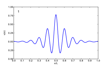
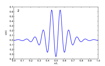
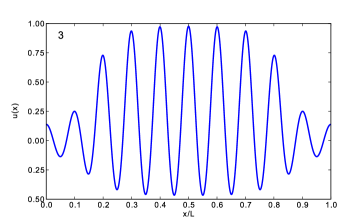
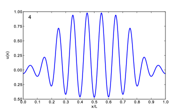
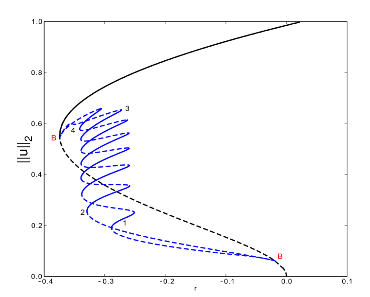
Figure 1: Homoclinic snaking for the SHE. Upper panel: bifurcation diagram showing branches of periodic patterns (black) and localised states (blue) in the (r,u2)𝑟subscriptnorm𝑢2(r,||u||_{2})-plane for the N23subscript𝑁23N_{23} SHE, for b=1.8𝑏1.8b=1.8. Solid (dashed) lines indicate stable (unstable) solutions. Points marked ‘B’ are the bifurcations at which the localised states emerge from the periodic states and are a consequence of the finite computational domain. Lower panels: illustrative solution profiles u(x,t)𝑢𝑥𝑡u(x,t) at the four numbered locations on the bifurcation diagram. The domain length used is 0x20π0𝑥20𝜋0\leq x\leq 20\pi, with periodic boundary conditions. This figure, and several others, was computed using the continuation software AUTO [14].

When the initial bifurcation at r=0𝑟0r=0 is subcritical, the patterned branch undergoes a saddle-node bifurcation at finite amplitude in r<0𝑟0r<0 in both versions of the SHE, illustrated for the N23subscript𝑁23N_{23} case in figure 1. In a finite domain, additional bifurcation points (labelled ‘B’ in the figure) arise along the branch. In a finite domain these bifurcation points are connected by intertwining branches of modulated solutions that become increasingly localised as the domain size increases. The formation of these intertwining curves is therefore often referred to as ‘homoclinic snaking’, an (at first sight) unusual structure that has a rich theoretical background as discussed by many authors [6, 9, 4]. Figure 1 also shows typical solution profiles at the top and bottom of each snaking curve. The snaking curves characterise the set of stationary solutions where u(x)𝑢𝑥u\left(x\right) describes an orbit that is spatially homoclinic to the state u(x)0𝑢𝑥0u(x)\equiv 0 after exactly one excursion near the periodic pattern. The oscillations in each smooth curve are connected through a set of saddle-node bifurcations that ‘snake’ backwards and forwards between limiting values of r𝑟r. For the parameter values of figure 1 this is approximately the interval 0.34<r<0.260.34𝑟0.26-0.34<r<-0.26.

Within this snaking region lies a Maxwell point at which the periodic state is energetically equal to the background state, and therefore one would expect stationary fronts between them to be possible. Such a Maxwell point can only be defined for systems that are variational in structure. This is the case for the SHE, and the corresponding free energy quantity is

[u]=Ω(12uxx2ux2+1r2u2uN(s)𝑑s)𝑑x,delimited-[]𝑢subscriptΩ12superscriptsubscript𝑢𝑥𝑥2superscriptsubscript𝑢𝑥21𝑟2superscript𝑢2superscript𝑢𝑁𝑠differential-d𝑠differential-d𝑥\displaystyle\mathcal{F}[u]=\int_{\Omega}\left(\frac{1}{2}u_{xx}^{2}-u_{x}^{2}+\frac{1-r}{2}u^{2}-\int^{u}N(s)\ ds\right)\ dx,

so that ut=δ/δusubscript𝑢𝑡𝛿𝛿𝑢u_{t}=-\delta\mathcal{F}/\delta u and so

ddt=utδδu=(ut)20,𝑑𝑑𝑡𝑢𝑡𝛿𝛿𝑢superscriptsubscript𝑢𝑡20\displaystyle\frac{d\mathcal{F}}{dt}=\frac{\partial u}{\partial t}\frac{\delta\mathcal{F}}{\delta u}=-\left(u_{t}\right)^{2}\leq 0,

which guarantees convergence to equilibrium states, as long as [u]delimited-[]𝑢\mathcal{F}[u] is bounded from below. As one moves up the snake, each additional crossing back-and-forth on the bifurcation diagram is associated with the creation of an additional pair of large amplitude peaks, one at each edge of the localised pattern; solutions at the top of the snake are wider than those at the bottom and the number of turns on the snake is proportional to the size of the domain. In addition to the curves shown in figure 1 there are stationary asymmetric states that exist on ‘rungs’ that link the two intertwining curves together. The rungs emerge in pitchfork bifurcations near to the saddle-node bifurcation points on the snaking curves. The rung states closely resemble the symmetric localised states on the snaking curves but they have a different phase relation between the small-scale periodic spatial oscillations and their overall envelope. For the SHE they are always unstable. The detailed description of the snaking curves and rung branches demands a close examination of the role of the relative phase between the small-scale and the envelope and this can only be done, in an asymptotic approach, by considering terms that are formally exponentially small. The form of these exponentially small terms has been studied using both exponential asymptotics [19, 7, 13] and the variational approximation method [24, 21, 12].

2.1 Multiple scales asymptotics for the SHE

In this section we review the results of the well-known multiple scales computations for the N23subscript𝑁23N_{23} and N35subscript𝑁35N_{35} cases of the SHE. To make progress we consider a perturbation expansion that considers small amplitude solutions, introducing the parameter ε𝜀\varepsilon to describe the solution amplitude:

u(x,t)=εu1+ε2u2+ε3u3+ε4u4+ε5u5+.𝑢𝑥𝑡𝜀subscript𝑢1superscript𝜀2subscript𝑢2superscript𝜀3subscript𝑢3superscript𝜀4subscript𝑢4superscript𝜀5subscript𝑢5u\left(x,t\right)=\varepsilon u_{1}+\varepsilon^{2}u_{2}+\varepsilon^{3}u_{3}+\varepsilon^{4}u_{4}+\varepsilon^{5}u_{5}+\cdots. (2.2)

In addition, the scalar field u(x,t)𝑢𝑥𝑡u(x,t) is modelled as evolving on two different length scales near the bifurcation at r=0𝑟0r=0: u(x,t)𝑢𝑥𝑡u(x,t) comprises a periodic function on the short lengthscale x𝑥x, modulated by an unknown envelope A(X)𝐴𝑋A(X) that is a function of a long lengthscale X𝑋X. In general one would also assume that the two components evolve on different timescales: the underlying pattern varying on the short timescale t𝑡t, and the envelope evolving on a long timescale T𝑇T. Since the instability at r=0𝑟0r=0 is steady, the dependence on t𝑡t is in fact trivial. We therefore look for leading-order solutions in the form

u1(x,X,t,T)=A(X,T)eix+A¯(X,T)eix,subscript𝑢1𝑥𝑋𝑡𝑇𝐴𝑋𝑇superscripte𝑖𝑥¯𝐴𝑋𝑇superscripte𝑖𝑥u_{1}\left(x,X,t,T\right)=A\left(X,T\right)\mathrm{e}^{ix}+\bar{A}\left(X,T\right)\mathrm{e}^{-ix}, (2.3)

where we add the complex conjugate so that u1subscript𝑢1u_{1} is real even though A(X,T)𝐴𝑋𝑇A(X,T) may be complex-valued. Our last requirement is that the bifurcation parameter r𝑟r is small which in turn demands that r𝑟r is rescaled: the rescaled parameter is denoted μ𝜇\mu.

We will consider two different sets of parameter scalings. For the SHE the results of the multiple scales calculations are well-known and we give only the results. These provide useful comparisons with the results for the nonlocal SHE presented in section 3. The first set of scalings leads to a solvability condition being imposed at O(ε3)𝑂superscript𝜀3O(\varepsilon^{3}) in the multiple scales expansion, and results in an envelope equation that can be solved analytically using Jacobi elliptic functions. The second set of scalings does not require a solvability condition being imposed before O(ε5)𝑂superscript𝜀5O(\varepsilon^{5}). Although this analysis generates a PDE that does not, in general, have closed form equilibrium solutions, it does provide a leading order estimate of the location of the snaking curves in the bifurcation diagram.

2.2 Derivation of a Ginzburg–Landau equation at third order

The first set of scalings considered is:

X=εx;T=ε2t;r=ε2μ.formulae-sequence𝑋𝜀𝑥formulae-sequence𝑇superscript𝜀2𝑡𝑟superscript𝜀2𝜇\displaystyle X=\varepsilon x;\qquad\qquad T=\varepsilon^{2}t;\qquad\qquad r=\varepsilon^{2}\mu. (2.4)

Proceeding with the standard multiple scales technique of substituting (2.2) into (1.1) and solving for un(x,X,t,T)subscript𝑢𝑛𝑥𝑋𝑡𝑇u_{n}(x,X,t,T) at successive orders in ε𝜀\varepsilon we derive evolution equations for A(X,T)𝐴𝑋𝑇A(X,T), in both the N23subscript𝑁23N_{23} and N35subscript𝑁35N_{35} cases, through the solvability conditions that arise at O(ε3)𝑂superscript𝜀3O(\varepsilon^{3}). For the N23subscript𝑁23N_{23} case we obtain

AT=μA+389(b22738)A|A|2+4AXX,subscript𝐴𝑇𝜇𝐴389superscript𝑏22738𝐴superscript𝐴24subscript𝐴𝑋𝑋A_{T}=\mu A+\frac{38}{9}\left(b^{2}-\frac{27}{38}\right)A\left|A\right|^{2}+4A_{XX}, (2.5)

and for the N35subscript𝑁35N_{35} case we obtain

AT=μA+3sA|A|2+4AXX.subscript𝐴𝑇𝜇𝐴3𝑠𝐴superscript𝐴24subscript𝐴𝑋𝑋A_{T}=\mu A+3sA\left|A\right|^{2}+4A_{XX}. (2.6)

The behaviour and solutions of these cubic Ginzburg–Landau equations are discussed in many places, for example [27] and [16]. The cubic GL equations have explicit solutions in terms of Jacobi elliptic functions. Of more interest for our purposes is that the coefficient of the nonlinear term vanishes in the cases b2=2738superscript𝑏22738b^{2}=\frac{27}{38} and s=0𝑠0s=0; at these parameter values the pattern-forming instability switches between supercritical and subcritical. Examination of the codimension-two points (r,b)=(0,27/38)𝑟𝑏02738(r,b)=(0,\sqrt{27/38}) and (r,s)=(0,0)𝑟𝑠00(r,s)=(0,0) allows us to extend the multiple scales analysis to include the restabilisation of periodic patterns at larger amplitudes; this is considered in the next section.

2.3 Derivation of a Ginzburg–Landau Equation at fifth order

To examine the codimension-two points at which the instability at r=0𝑟0r=0 switches from supercritical to subcritical we rescale the coefficient of the nonlinear term with the lower exponent, writing

b=2738+ε2b2;ors=ε2s2,formulae-sequence𝑏2738superscript𝜀2subscript𝑏2or𝑠superscript𝜀2subscript𝑠2b=\sqrt{\frac{27}{38}}+\varepsilon^{2}b_{2};\qquad\mathrm{or}\qquad s=\varepsilon^{2}s_{2}, (2.7)

in the N23subscript𝑁23N_{23} and N35subscript𝑁35N_{35} cases, respectively. To balance the linear terms in (2.5) and (2.6) at a higher order in the expansion, we introduce the alternative set of scalings

X=ε2x;T=ε4t;r=ε4μ.formulae-sequence𝑋superscript𝜀2𝑥formulae-sequence𝑇superscript𝜀4𝑡𝑟superscript𝜀4𝜇X=\varepsilon^{2}x;\qquad\qquad T=\varepsilon^{4}t;\qquad\qquad r=\varepsilon^{4}\mu. (2.8)

No secular terms are generated before O(ε5)𝑂superscript𝜀5O\left(\varepsilon^{5}\right). At O(ε5)𝑂superscript𝜀5O(\varepsilon^{5}) we obtain cubic-quintic Ginzburg–Landau equations as follows. For the N23subscript𝑁23N_{23} case we obtain

AT=μA+23114b2A|A|28820361A|A|4+i1619AX|A|2+4AXX,subscript𝐴𝑇𝜇𝐴23114subscript𝑏2𝐴superscript𝐴28820361𝐴superscript𝐴4𝑖1619subscript𝐴𝑋superscript𝐴24subscript𝐴𝑋𝑋A_{T}=\mu A+\frac{2}{3}\sqrt{114}b_{2}A\left|A\right|^{2}-\frac{8820}{361}A\left|A\right|^{4}+i\frac{16}{19}A_{X}\left|A\right|^{2}+4A_{XX}, (2.9)

and for the N35subscript𝑁35N_{35} case we obtain

AT=μA+3s2A|A|210A|A|4+4AXX.subscript𝐴𝑇𝜇𝐴3subscript𝑠2𝐴superscript𝐴210𝐴superscript𝐴44subscript𝐴𝑋𝑋A_{T}=\mu A+3s_{2}A\left|A\right|^{2}-10A\left|A\right|^{4}+4A_{XX}. (2.10)

The linear terms are identical to those in (2.5) and (2.6), but the different scalings bring additional nonlinear terms into the asymptotic balance.

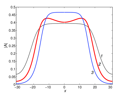
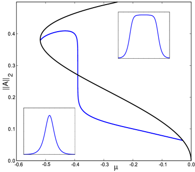
The cubic-quintic Ginzburg–Landau equations (2.9) and (2.10) derived at O(ε5)𝑂superscript𝜀5O(\varepsilon^{5}) are able to capture the bistability through their more complicated collection of competing nonlinear terms. This is illustrated in figure 2.

Figure 2 is clearly similar in structure to figure 1 in that a modulated branch (blue) bifurcates from the primary solution branch (black) at two points, one close to μ=0𝜇0\mu=0 and one close to the saddle node bifurcation. The vertical section of the modulated branch indicates the Maxwell point at which the envelope increases rapidly over a very small range of μ𝜇\mu. We note that the cubic-quintic Ginzburg–Landau equation (2.9) and its more general counterparts have been recently investigated by Kao and Knobloch [18] in some detail.
Refer to caption
Figure 2: Bifurcation diagram in the (μ,A2)𝜇subscriptnorm𝐴2(\mu,\|A\|_{2}) plane for the cubic-quintic Ginzburg–Landau equation (2.9) for b2=1subscript𝑏21b_{2}=1 showing the homogeneous (black) and modulated (blue) branches of solutions. The inset figures indicate the general shape of the modulus of the amplitude |A(X)|𝐴𝑋|A(X)| at two points low down (μ0.1𝜇0.1\mu\approx-0.1) and higher up (μ0.4𝜇0.4\mu\approx-0.4) on the blue curve. The domain used is 0X20π0𝑋20𝜋0\leq X\leq 20\pi, with periodic boundary conditions.

3 Including a nonlocal term

Having summarised the usual asymptotic analysis of the local SHE, we now extend it to the case in which an additional nonlinear nonlocal term exists. Specifically we consider the nonlocal Swift–Hohenberg equation

tu=[r(1+x2)2]u+N(u)γu(x,t)ΩK(xy)u(y,t)2𝑑y,subscript𝑡𝑢delimited-[]𝑟superscript1superscriptsubscript𝑥22𝑢𝑁𝑢𝛾𝑢𝑥𝑡subscriptΩ𝐾𝑥𝑦𝑢superscript𝑦𝑡2differential-d𝑦\displaystyle\partial_{t}u=\left[r-(1+\partial_{x}^{2})^{2}\right]u+N(u)-\gamma u(x,t)\int_{\Omega}K\left(x-y\right)u\left(y,t\right)^{2}\,dy, (3.1)

where K(x)𝐾𝑥K(x) is a bounded function defined on ΩΩ\Omega that either has bounded support, or decays sufficiently rapidly at large |x|𝑥|x|, so that its Fourier transform exists. These properties define what we mean by ‘short range’: we treat the form of K(x)𝐾𝑥K(x) and any parameters on which it depends as fixed while working asymptotically in the limit ε1much-less-than𝜀1\varepsilon\ll 1.

3.1 Properties of K(x)𝐾𝑥K(x) and the free energy [u]delimited-[]𝑢\mathcal{F}[u]

We assume also that (i) K𝐾K is normalised so that ΩK(x)𝑑x=1subscriptΩ𝐾𝑥differential-d𝑥1\int_{\Omega}K(x)\ dx=1; (ii) K𝐾K is even: K(x)=K(x)xΩformulae-sequence𝐾𝑥𝐾𝑥for-all𝑥ΩK(x)=K(-x)\ \ \forall x\in\Omega, and (iii) K𝐾K is non-negative: K(x)0xΩformulae-sequence𝐾𝑥0for-all𝑥ΩK(x)\geq 0\ \ \forall x\in\Omega. The parameter γ𝛾\gamma is the coefficient of the nonlocal term. The form of the nonlinear nonlocal term proposed in (3.1) is motivated naturally from consideration of the free energy functional

[u]=Ω(12uxx2ux2+1r2u2uN(v)𝑑v)𝑑x+γ4ΩΩK(xy)u(x)2u(y)2𝑑x𝑑y.delimited-[]𝑢subscriptΩ12superscriptsubscript𝑢𝑥𝑥2superscriptsubscript𝑢𝑥21𝑟2superscript𝑢2superscript𝑢𝑁𝑣differential-d𝑣differential-d𝑥𝛾4subscriptΩsubscriptΩ𝐾𝑥𝑦𝑢superscript𝑥2𝑢superscript𝑦2differential-d𝑥differential-d𝑦\displaystyle\mathcal{F}[u]=\int_{\Omega}\left(\frac{1}{2}u_{xx}^{2}-u_{x}^{2}+\frac{1-r}{2}u^{2}-\int^{u}N(v)\ dv\right)\,dx+\frac{\gamma}{4}\int_{\Omega}\int_{\Omega}K(x-y)u(x)^{2}u(y)^{2}\,dx\ dy.

In order to check that the time evolution ut=δ/δusubscript𝑢𝑡𝛿𝛿𝑢u_{t}=-\delta\mathcal{F}/\delta u is well-posed, we need to ensure that \mathcal{F} is bounded below. In the cubic-quintic case N(u)=su3u5𝑁𝑢𝑠superscript𝑢3superscript𝑢5N(u)=su^{3}-u^{5} this is true for all real values of γ𝛾\gamma. In the quadratic-cubic case N(u)=bu2u3𝑁𝑢𝑏superscript𝑢2superscript𝑢3N(u)=bu^{2}-u^{3} we require γ>1𝛾1\gamma>-1 for \mathcal{F} to be bounded below. These conclusions follow from the following estimate on the size of the nonlocal term in \mathcal{F}, deduced by combining the Cauchy–Schwarz inequality and Young’s inequality for convolutions. Details of these inequalities can be found, for example, in the textbook by Lieb and Loss [20]. Since the nonlocal term is non-negative we have

ΩΩK(xy)u(x)2u(y)2𝑑x𝑑ysubscriptΩsubscriptΩ𝐾𝑥𝑦𝑢superscript𝑥2𝑢superscript𝑦2differential-d𝑥differential-d𝑦\displaystyle\int_{\Omega}\int_{\Omega}K(x-y)u(x)^{2}u(y)^{2}\,dx\ dy \displaystyle\equiv (Ku2)u21subscriptnorm𝐾superscript𝑢2superscript𝑢21\displaystyle\|(K\ast u^{2})u^{2}\|_{1} (3.2)
\displaystyle\leq Ku22u22subscriptnorm𝐾superscript𝑢22subscriptnormsuperscript𝑢22\displaystyle\|K\ast u^{2}\|_{2}\ \|u^{2}\|_{2}
\displaystyle\leq K1u22u22subscriptnorm𝐾1subscriptnormsuperscript𝑢22subscriptnormsuperscript𝑢22\displaystyle\left\|K\right\|_{1}\ \|u^{2}\|_{2}\ \|u^{2}\|_{2}
\displaystyle\leq Ωu(x)4𝑑x,subscriptΩ𝑢superscript𝑥4differential-d𝑥\displaystyle\int_{\Omega}u(x)^{4}\,dx,

where we adopt the usual notation fp:=(Ω|f|p𝑑x)1/passignsubscriptnorm𝑓𝑝superscriptsubscriptΩsuperscript𝑓𝑝differential-d𝑥1𝑝\|f\|_{p}:=\left(\int_{\Omega}|f|^{p}\,dx\right)^{1/p} for the p𝑝p-norm of a function f(x)𝑓𝑥f(x), and we have used Cauchy–Schwarz to derive the second line, Young’s inequality for the third line, and the fact that K1=1subscriptnorm𝐾11\|K\|_{1}=1 (normalisation) for the fourth line. As a result we can see that in [u]delimited-[]𝑢\mathcal{F}[u] in the cubic-quintic case the nonlocal term is always dominated by the 16u616superscript𝑢6\frac{1}{6}u^{6} term in [u]delimited-[]𝑢\mathcal{F}[u]. In the quadratic-cubic case with γ>0𝛾0\gamma>0 we see that the nonlocal term makes a non-negative contribution to [u]delimited-[]𝑢\mathcal{F}[u]. In the remaining case, of quadratic-cubic terms with γ<0𝛾0\gamma<0, we can estimate that

[u]Ω12(uxx+u)2r2u2b3u3+14(1|γ|)u4dxdelimited-[]𝑢subscriptΩ12superscriptsubscript𝑢𝑥𝑥𝑢2𝑟2superscript𝑢2𝑏3superscript𝑢3141𝛾superscript𝑢4𝑑𝑥\displaystyle\mathcal{F}[u]\geq\int_{\Omega}\frac{1}{2}(u_{xx}+u)^{2}-\frac{r}{2}u^{2}-\frac{b}{3}u^{3}+\frac{1}{4}(1-|\gamma|)u^{4}\,dx

which follows after integrating the term ux2superscriptsubscript𝑢𝑥2-u_{x}^{2} by parts and using the estimate (3.2). Hence

[u]Ωb3u3+14(1|γ|)u4dx,delimited-[]𝑢subscriptΩ𝑏3superscript𝑢3141𝛾superscript𝑢4𝑑𝑥\displaystyle\mathcal{F}[u]\geq\int_{\Omega}-\frac{b}{3}u^{3}+\frac{1}{4}(1-|\gamma|)u^{4}\,dx,

which is bounded below, per unit length of the domain ΩΩ\Omega, by b4/(12(1|γ|)3)superscript𝑏412superscript1𝛾3-b^{4}/(12(1-|\gamma|)^{3}). The bound γ>1𝛾1\gamma>-1 is strict since it is attained by the choice of kernel K(x)=δ(x)𝐾𝑥𝛿𝑥K(x)=\delta(x) the ‘Dirac delta’ distribution.

3.2 Limiting choices for K(x)𝐾𝑥K(x)

There are two limiting choices of K(x)𝐾𝑥K(x) for which the behaviour of solutions to (3.1) can be determined by inspection. The first is the case where K(x)1|Ω|𝐾𝑥1ΩK(x)\equiv\frac{1}{|\Omega|}, referred to as ‘global coupling’ in [15]. In this case the bifurcation parameter r𝑟r is effectively replaced by the new parameter r=rγu2superscript𝑟𝑟𝛾delimited-⟨⟩superscript𝑢2r^{\prime}=r-\gamma\left\langle u^{2}\right\rangle where the angled brackets indicate the domain-averaged integral: u2:=1|Ω|Ωu(x,t)2𝑑x1|Ω|u22assigndelimited-⟨⟩superscript𝑢21ΩsubscriptΩ𝑢superscript𝑥𝑡2differential-d𝑥1Ωsuperscriptsubscriptnorm𝑢22\langle u^{2}\rangle:=\frac{1}{|\Omega|}\int_{\Omega}u(x,t)^{2}dx\equiv\frac{1}{|\Omega|}\|u\|_{2}^{2}. As noted in [15], in this case there is a correspondence between solutions ulocalsubscript𝑢𝑙𝑜𝑐𝑎𝑙u_{local} and unonlocalsubscript𝑢𝑛𝑜𝑛𝑙𝑜𝑐𝑎𝑙u_{nonlocal} of the local and nonlocal problems, respectively, given by changing the parameter value:

unonlocal(x,t;r,γ)=ulocal(x,t;rγu2).subscript𝑢𝑛𝑜𝑛𝑙𝑜𝑐𝑎𝑙𝑥𝑡superscript𝑟𝛾subscript𝑢𝑙𝑜𝑐𝑎𝑙𝑥𝑡𝑟𝛾delimited-⟨⟩superscript𝑢2u_{nonlocal}\left(x,t;r^{\prime},\gamma\right)=u_{local}\left(x,t;r-\gamma\left\langle u^{2}\right\rangle\right). (3.3)

The second limiting case is where K(x)=δ(x)𝐾𝑥𝛿𝑥K(x)=\delta\left(x\right), a ‘Dirac delta’ function. This case amounts to only a change in the nonlinearity from N(u)𝑁𝑢N(u) to N(u)+γu3𝑁𝑢𝛾superscript𝑢3N(u)+\gamma u^{3}, i.e. in the N23subscript𝑁23N_{23} and N35subscript𝑁35N_{35} cases the coefficient of the cubic term is increased by γ𝛾\gamma.

Refer to caption
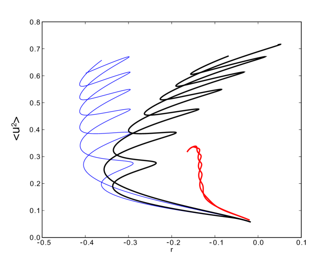
Figure 3: Homoclinic snaking in local and global cases of the (2–3) Swift–Hohenberg equation (3.1). Homoclinic snaking curves in the (r,u2)𝑟subscriptnorm𝑢2(r,\|u\|_{2}) plane are shown for the local case (blue, thin line), and for the nonlocal case (3.1) in the limiting cases K(x)=δ(x)𝐾𝑥𝛿𝑥K(x)=\delta\left(x\right) (red, right-hand curves), and K=1L𝐾1𝐿K=\frac{1}{L} (black, sloping curves). Parameter values are γ=0.7𝛾0.7\gamma=0.7, b=1𝑏1b=1. A domain size L=20π𝐿20𝜋L=20\pi and periodic boundary conditions were used. Stability is not indicated.

Figure 3 illustrates the snaking curves for the N23subscript𝑁23N_{23} case, for fixed values of the parameters b𝑏b and γ𝛾\gamma, varying the choice of kernel function. It confirms the observations made in the paragraph above: the global coupling case results in a slanted version of the snake from the local problem: they can be mapped onto each other via the relation (3.3). The choice of the Dirac delta function for the kernel produces the smaller snake at r𝑟r closer to zero: it is vertical rather than slanted since effectively only the coefficient of u3superscript𝑢3u^{3} has been altered. Since for a general kernel K(x)𝐾𝑥K(x), the nonlocal problem cannot be related directly to a simple transformation of the local problem, and detailed analysis is necessary, the remainder of this paper can be thought of as understanding how the snake shifts between these two limiting cases.

3.3 Homoclinic snaking in the nonlocal SHE
Refer to caption
Refer to caption
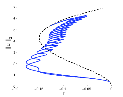
Figure 4: Homoclinic snaking in the nonlocal N23subscript𝑁23N_{23} Swift–Hohenberg equation (3.1) with the Gaussian kernel KG(x)subscript𝐾𝐺𝑥K_{G}(x) defined in (3.4). Homoclinic snaking curves on which the localised states lie are shown as solid blue lines. Dashed black lines indicate the location of spatially periodic solutions. (a) σ=4π𝜎4𝜋\sigma=4\pi; (b) σ=10π𝜎10𝜋\sigma=10\pi. Other parameter values are γ=0.5𝛾0.5\gamma=0.5, b=1.6𝑏1.6b=1.6, domain size L=40π𝐿40𝜋L=40\pi. Periodic boundary conditions were used, and stability is not indicated.

When the kernel K(x)𝐾𝑥K(x) is assumed either to decay very rapidly, or to decay very slowly compared to the (finite) size of the domain ΩΩ\Omega, we might propose that the effect of the nonlocal term is only to shift the snaking curves in r𝑟r a little from the purely local or purely global problem, respectively. Figure 4 presents bifurcation diagrams for the snaking curves in each of these cases, using the Gaussian kernel

KG(x)subscript𝐾𝐺𝑥\displaystyle K_{G}\left(x\right) =\displaystyle= 12πσ2ex2/(2σ2).12𝜋superscript𝜎2superscriptesuperscript𝑥22superscript𝜎2\displaystyle\frac{1}{\sqrt{2\pi\sigma^{2}}}\mathrm{e}^{-x^{2}/(2\sigma^{2})}. (3.4)

In figure 4(a) the width of the Gaussian kernel is σ=4π𝜎4𝜋\sigma=4\pi which is small compared to the domain size L=40π𝐿40𝜋L=40\pi. The first few turns on the snake are shifted to lower r𝑟r and the last few slightly shifted to higher r𝑟r, while the centre of the snake remains close to vertical. Figure 4(b) contains the corresponding snaking bifurcation diagram for σ=10π𝜎10𝜋\sigma=10\pi in the same size domain L=40π𝐿40𝜋L=40\pi. The homoclinic snaking is stretched out in a manner similar to slanted snaking, but with an overall ‘S’ shape that the purely global term cannot generate.
Refer to caption
Refer to caption
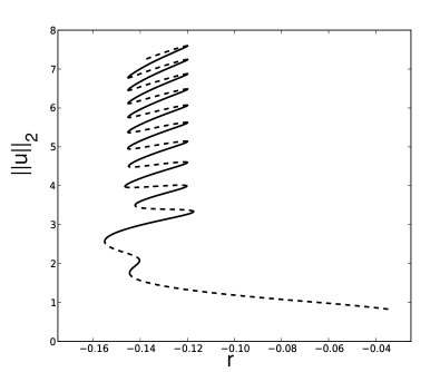
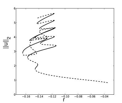
Figure 5: Bifurcation diagrams in the (r,u2)𝑟subscriptnorm𝑢2(r,\|u\|_{2}) plane illustrating homoclinic snaking in the nonlocal N23subscript𝑁23N_{23} Swift–Hohenberg equation (3.1) with the top hat kernel KTH(x)subscript𝐾𝑇𝐻𝑥K_{TH}(x) defined in (3.5). (a) δ=36𝛿36\delta=36; (b) δ=38𝛿38\delta=38. Other parameter values are γ=0.5𝛾0.5\gamma=0.5, b=1.6𝑏1.6b=1.6, domain size L=40π𝐿40𝜋L=40\pi. Periodic boundary conditions were used, and solid (dashed) lines indicate stable (unstable) solutions.
Refer to caption
Refer to captionRefer to captionRefer to captionRefer to caption
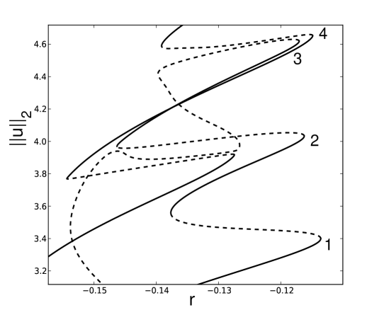
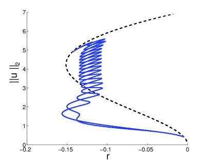
Figure 6: Homoclinic snaking in nonlocal versions of the N23subscript𝑁23N_{23} Swift–Hohenberg equation (3.1) with a top hat kernel KTH(x)subscript𝐾𝑇𝐻𝑥K_{TH}(x). (a) Enlargement of figure 5(b); (b) solution profiles at the four points labelled 111444 in (a). Other parameter values are γ=0.5𝛾0.5\gamma=0.5, b=1.6𝑏1.6b=1.6, domain size L=40π𝐿40𝜋L=40\pi. Periodic boundary conditions were used, and solid (dashed) lines indicate stable (unstable) solutions.

It is surprising that the transition between figure 4(a) and figure 4(b) as the width parameter σ𝜎\sigma increases does not occur in the obvious fashion that one might expect, with the snaking curves deforming smoothly from one figure to the other. Instead, it appears to be a complicated process in which the snaking curves collide with other solution branches, consisting of multipulse states, and re-connect before pinching off again as σ𝜎\sigma increases further. To illustrate this complex process, figures 5 and 6 present some of the details of the initial changes in bifurcation structure as the kernel width increases, in this case for the top hat kernel

KTH(x)subscript𝐾𝑇𝐻𝑥\displaystyle K_{TH}\left(x\right) =\displaystyle= 1δ[H(x+δ2)H(xδ2)],1𝛿delimited-[]𝐻𝑥𝛿2𝐻𝑥𝛿2\displaystyle\frac{1}{\delta}\left[H\left(x+\frac{\delta}{2}\right)-H\left(x-\frac{\delta}{2}\right)\right], (3.5)

where H(x)𝐻𝑥H(x) denotes the Heaviside function: H(x)=0𝐻𝑥0H(x)=0 if x0𝑥0x\leq 0 and H(x)=1𝐻𝑥1H(x)=1 if x>0𝑥0x>0. Figure 5(a) shows the lower end of one of the snaking branches at δ=36𝛿36\delta=36; this value of δ𝛿\delta should be considered narrow compared to the overall domain width L=40π𝐿40𝜋L=40\pi. Figure 5(b) is computed in the same way for the slightly increased value δ=38𝛿38\delta=38. The snaking curve has collided with two isolas, leading to a number of additional loops over which the solution amplitude, as measured by the L2subscript𝐿2L_{2} norm, decreases. Such loops were referred to as ‘switchbacks’ by Taylor & Dawes [25]. Figure 6(a) is an enlargement of part of figure 5(b) that shows the reconnection of several parts of the snaking curve to link to the isolas. Figure 6(b) presents plots of the solution u(x)𝑢𝑥u(x) at the four saddle-node bifurcation points on the right-hand side of figure 6(a), in sequence as the L2subscript𝐿2L_{2} norm increases. Despite the upper pair occurring very close to each other both in L2subscript𝐿2L_{2} norm and values of r𝑟r, the solutions look very different: the upper one is clearly related to a multipulse localised state. Very similar behaviour is observed for the Gaussian kernel; the formation of switchbacks in general appears not to be related to the choice of kernel.

Figures 3 and 4 lay out the challenges that we analyse in detail in the remainder of the paper: developing the well-known multiple-scale analysis to include nonlocal terms allows us to determine the location of the branches of localised states and captures the ‘S’ shaped nature of the branches as shown in figure 4. As is also well-known, the regular multiple-scales analysis does not shed light on the behaviour of individual snaking curves, and so we are unable to say anything analytic about the breakup of the snaking curves and the collisions with branches of multipulse states that are clearly shown in figures 5 and 6. We suspect that the details of these collisions are strongly dependent on the precise form chosen for the kernel K(x)𝐾𝑥K(x) and we leave these details to be the subject of future work.
Refer to caption
Refer to caption
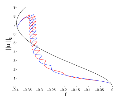
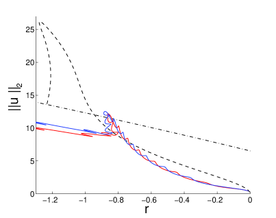
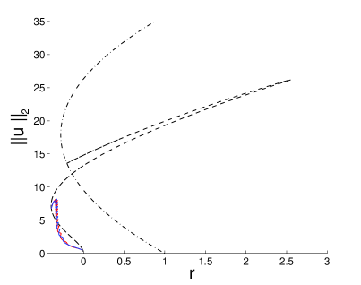
Figure 7: Left: Bifurcation diagram for solutions of the nonlocal Swift–Hohenberg equation (3.1) with a Gaussian kernel, for γ=0.5𝛾0.5\gamma=-0.5. Dashed line indicates the branch of spatially periodic states that bifurcates from the trivial state at r=0𝑟0r=0. Dashed-dotted line indicates the non-zero constant state that bifurcates from the trivial state at r=1𝑟1r=1. Solid (red and blue) curves are the branches of localised states. Stability is not shown. Other parameter values are σ=4π𝜎4𝜋\sigma=4\pi, b=1.6𝑏1.6b=1.6, domain size L=40π𝐿40𝜋L=40\pi.
Refer to caption
Refer to caption
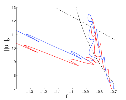
Figure 8: Left: Bifurcation diagram for solutions of the nonlocal Swift–Hohenberg equation (3.1) with a Gaussian kernel, for γ=1.2𝛾1.2\gamma=-1.2. Dashed line indicates the branch of spatially periodic states that bifurcates from the trivial state at r=0𝑟0r=0. Dashed-dotted line indicates the non-zero constant state that bifurcates from the trivial state at r=1𝑟1r=1. Solid (red and blue) curves are the branches of localised states. Stability is not shown. Other parameter values are σ=4π𝜎4𝜋\sigma=4\pi, b=1.6𝑏1.6b=1.6, domain size L=40π𝐿40𝜋L=40\pi.

Finally, figures 7 and 8 show results for γ=0.5𝛾0.5\gamma=-0.5 and γ=1.2𝛾1.2\gamma=-1.2, respectively, using the Gaussian kernel KG(x)subscript𝐾𝐺𝑥K_{G}(x) with σ=4π𝜎4𝜋\sigma=4\pi. The case γ=0.5𝛾0.5\gamma=-0.5 shows standard homoclinic snaking with branches of localised states reconnecting to the spatially periodic branch near its usual saddle-node bifurcation as the localised state expands to fill the entire domain. One might expect the snaking curves to be tilted backwards, which they are at the lower end but they remain vertical in the central section, as in the case γ=0.5𝛾0.5\gamma=0.5 shown in figure 4(a). Figure 7 shows that the branch of spatially periodic states that bifurcates from r=0𝑟0r=0 (and shown as a dashed line) extends into r>0𝑟0r>0 before turning round at a second saddle-node point and then terminating on the branch of non-zero spatially constant states (shown as the dash-dotted line) that bifurcates from r=1𝑟1r=1. This point is therefore another Turing-type instability, this time of the non-zero constant solution.

Numerical investigations reveal that the usual homoclinic snaking structure persists, for σ=4π𝜎4𝜋\sigma=4\pi, down to around γ=1.13𝛾1.13\gamma=-1.13 and certainly into γ<1𝛾1\gamma<-1. But below a critical value, the localised states undergo new instabilities in which the central peaks of the localised state widen significantly. These snaking curves do not reconnect to the periodic branch, but instead extend into negative r𝑟r, undergoing a number of additional twists and turns. This behaviour is illustrated in figure 8. We remark also that taking γ𝛾\gamma large and negative changes the behaviour of the constant and spatially periodic branches: in figure 8 we observe that the branch of spatially periodic states (dashed line) evolves monotonically until reaching a first saddle-node bifurcation at r1.2𝑟1.2r\approx-1.2, and that the branch of positive constant solutions (dash-dotted line) extends into r<0𝑟0r<0 and does not undergo a saddle-node bifurcation.

4 Derivation of cubic Ginzburg–Landau equations

In this section we discuss the construction of amplitude equations in the simplest case, in which the kernel K(x)𝐾𝑥K(x) varies only on the short length scale. Equivalently, this is the case where all terms posed on the long length scale X𝑋X are assumed to be almost constant over the region where the kernel is large. This makes sense in the case that the envelope function is smooth and the kernel function decays much more rapidly than the envelope; hence on functions of X𝑋X, the kernel K(x)𝐾𝑥K(x) acts to leading order in ε𝜀\varepsilon, as a Dirac δ𝛿\delta-distribution. This statement will be made more precise in section 5.1 below. For the moment we will illustrate the computations involved in deriving the modifications to the cubic Ginzburg–Landau equations (2.5) and (2.6) when the nonlocal term is included.

Within the weakly nonlinear multiple scales expansion (2.2), we can see by inspection that the presence of the nonlinear nonlocal term contributes only at O(ε3)𝑂superscript𝜀3O(\varepsilon^{3}) and higher. Direct substitution of the ansatz (2.2) into the nonlocal term indicates that, at the orders in ε𝜀\varepsilon that are of interest in deriving the solvability conditions at third or fifth order in ε𝜀\varepsilon, the following terms need to be evaluated:

O(ε3)::𝑂superscript𝜀3absent\displaystyle O\left(\varepsilon^{3}\right):\ \ 3:=u1(x)J11,assignsubscript3subscript𝑢1𝑥subscript𝐽11\displaystyle\mathcal{I}_{3}:=u_{1}\left(x\right)J_{11}, (4.1)
O(ε4)::𝑂superscript𝜀4absent\displaystyle O\left(\varepsilon^{4}\right):\ \ 4:=u2(x)J11+2u1(x)J12,assignsubscript4subscript𝑢2𝑥subscript𝐽112subscript𝑢1𝑥subscript𝐽12\displaystyle\mathcal{I}_{4}:=u_{2}\left(x\right)J_{11}+2u_{1}(x)J_{12}, (4.2)
O(ε5)::𝑂superscript𝜀5absent\displaystyle O\left(\varepsilon^{5}\right):\ \ 5:=u3(x)J11+2u2(x)J12,+u1(x)(2J13+J22),assignsubscript5subscript𝑢3𝑥subscript𝐽112subscript𝑢2𝑥subscript𝐽12subscript𝑢1𝑥2subscript𝐽13subscript𝐽22\displaystyle\mathcal{I}_{5}:=u_{3}\left(x\right)J_{11}+2u_{2}\left(x\right)J_{12},+u_{1}\left(x\right)\left(2J_{13}+J_{22}\right), (4.3)

where the integrals Jij(x)subscript𝐽𝑖𝑗𝑥J_{ij}(x) for i,j{1,2,3}𝑖𝑗123i,j\in\{1,2,3\} are defined to be

Jij(x):=ΩK(xy)ui(y)uj(y)𝑑y.assignsubscript𝐽𝑖𝑗𝑥subscriptΩ𝐾𝑥𝑦subscript𝑢𝑖𝑦subscript𝑢𝑗𝑦differential-d𝑦\displaystyle J_{ij}(x):=\int_{\Omega}K\left(x-y\right)u_{i}\left(y\right)u_{j}\left(y\right)\,dy. (4.4)

To simplify the presentation we will carry out the computations initially for two explicit kernel functions: the Gaussian KG(x)subscript𝐾𝐺𝑥K_{G}(x) defined in (3.4) and the piecewise-constant top hat function KTH(x)subscript𝐾𝑇𝐻𝑥K_{TH}(x) defined in (3.5). Since the scalings (2.4) generate secular terms at O(ε3)𝑂superscript𝜀3O(\varepsilon^{3}) and higher, for the cubic Ginzburg–Landau equations we need only to evaluate the leading-order part of the expression (4.1) and then incorporate any additional resonant terms (i.e. those having a short-scale dependence e±ixsimilar-toabsentsuperscripteplus-or-minusi𝑥\sim\mathrm{e}^{\pm\mathrm{i}x}) into the Ginzburg-Landau equations (2.5) and (2.6) derived previously. Substituting the ansatz (2.3) into (4.1) we obtain

J11subscript𝐽11\displaystyle J_{11} =\displaystyle= ΩK(xy)(2|A(Y)|2+A(Y)2e2iy+A¯(Y)2e2iy)𝑑y.subscriptΩ𝐾𝑥𝑦2superscript𝐴𝑌2𝐴superscript𝑌2superscripte2i𝑦¯𝐴superscript𝑌2superscripte2i𝑦differential-d𝑦\displaystyle\int_{\Omega}K\left(x-y\right)\left(2\left|A(Y)\right|^{2}+A(Y)^{2}\mathrm{e}^{2\mathrm{i}y}+\bar{A}(Y)^{2}\mathrm{e}^{-2\mathrm{i}y}\right)dy.

To determine the leading order contribution we consider the envelope A(Y)𝐴𝑌A(Y) to be constant within the integral, using the implicit decoupling of the short and long length scales x𝑥x and X=εx𝑋𝜀𝑥X=\varepsilon x that arises asymptotically as ε0𝜀0\varepsilon\rightarrow 0. We therefore obtain the leading order simplification

J11subscript𝐽11\displaystyle J_{11} =\displaystyle= 2|A(X)|2ΩK(xy)𝑑y+A(X)2ΩK(xy)e2iy𝑑y2superscript𝐴𝑋2subscriptΩ𝐾𝑥𝑦differential-d𝑦𝐴superscript𝑋2subscriptΩ𝐾𝑥𝑦superscripte2i𝑦differential-d𝑦\displaystyle 2\left|A(X)\right|^{2}\int_{\Omega}K\left(x-y\right)dy+A(X)^{2}\int_{\Omega}K\left(x-y\right)\mathrm{e}^{2\mathrm{i}y}dy (4.5)
+A¯(X)2ΩK(xy)e2iy𝑑y+O(ε).¯𝐴superscript𝑋2subscriptΩ𝐾𝑥𝑦superscripte2i𝑦differential-d𝑦𝑂𝜀\displaystyle+\bar{A}(X)^{2}\int_{\Omega}K\left(x-y\right)\mathrm{e}^{-2\mathrm{i}y}dy\ +O(\varepsilon).

We now evaluate these contributions in the cases of top hat and Gaussian kernels.

4.1 The top hat kernel KTH(x)subscript𝐾𝑇𝐻𝑥K_{TH}(x)

In this subsection we evaluate the integrals in (4.5) for the top hat kernel KTH(x)subscript𝐾𝑇𝐻𝑥K_{TH}(x) given in (3.5). The computations are the same regardless of the choice of a finite domain ΩΩ\Omega or an infinite domain Ω=Ω\Omega=\mathbb{R}, assuming that the width δ𝛿\delta of the support of KTH(x)subscript𝐾𝑇𝐻𝑥K_{TH}(x) is at most the domain length L𝐿L. Explicitly we obtain

J11subscript𝐽11\displaystyle J_{11} =\displaystyle= 2δ|A(X)|2xδ2x+δ2𝑑y+1δA(X)2xδ2x+δ2e2iy𝑑y+1δA(X)¯2xδ2x+δ2e2iy𝑑y.2𝛿superscript𝐴𝑋2superscriptsubscript𝑥𝛿2𝑥𝛿2differential-d𝑦1𝛿𝐴superscript𝑋2superscriptsubscript𝑥𝛿2𝑥𝛿2superscripte2𝑖𝑦differential-d𝑦1𝛿superscript¯𝐴𝑋2superscriptsubscript𝑥𝛿2𝑥𝛿2superscripte2𝑖𝑦differential-d𝑦\displaystyle\frac{2}{\delta}\left|A(X)\right|^{2}\intop_{x-\frac{\delta}{2}}^{x+\frac{\delta}{2}}dy+\frac{1}{\delta}A(X)^{2}\intop_{x-\frac{\delta}{2}}^{x+\frac{\delta}{2}}\mathrm{e}^{2iy}dy+\frac{1}{\delta}\bar{A(X)}^{2}\intop_{x-\frac{\delta}{2}}^{x+\frac{\delta}{2}}\mathrm{e}^{-2iy}dy.

Recall the general result, for integer m𝑚m, that

1δxδ2x+δ2eimy𝑑y=eimxsin(mδ/2)mδ/2,1𝛿superscriptsubscript𝑥𝛿2𝑥𝛿2superscripte𝑖𝑚𝑦differential-d𝑦superscripte𝑖𝑚𝑥𝑚𝛿2𝑚𝛿2\frac{1}{\delta}\intop_{x-\frac{\delta}{2}}^{x+\frac{\delta}{2}}\mathrm{e}^{imy}dy=\mathrm{e}^{imx}\frac{\sin\left(m\delta/2\right)}{m\delta/2}, (4.6)

which we use in the three cases m=2,0,2𝑚202m=-2,0,2 to obtain

J11subscript𝐽11\displaystyle J_{11} =\displaystyle= 2|A(X)|2+sinδδ(A(X)2e2ix+A(X)¯2e2ix).2superscript𝐴𝑋2𝛿𝛿𝐴superscript𝑋2superscripte2𝑖𝑥superscript¯𝐴𝑋2superscripte2𝑖𝑥\displaystyle 2\left|A(X)\right|^{2}+\frac{\sin\delta}{\delta}\left(A(X)^{2}\mathrm{e}^{2ix}+\bar{A(X)}^{2}\mathrm{e}^{-2ix}\right).

From J11subscript𝐽11J_{11} it is straightforward to compute 3subscript3\mathcal{I}_{3}:

3=(2+sinδδ)A|A|2eix+(sinδδ)A3e3ix+c.c.,formulae-sequencesubscript32𝛿𝛿𝐴superscript𝐴2superscripte𝑖𝑥𝛿𝛿superscript𝐴3superscripte3𝑖𝑥𝑐𝑐\mathcal{I}_{3}=\left(2+\frac{\sin\delta}{\delta}\right)A\left|A\right|^{2}\mathrm{e}^{ix}+\left(\frac{\sin\delta}{\delta}\right)A^{3}\mathrm{e}^{3ix}+c.c.,

where c.c.formulae-sequence𝑐𝑐c.c. denotes the complex conjugate, so that 3subscript3\mathcal{I}_{3} is always real-valued. Comparison with the calculations in the previous sections shows that in the presence of the nonlocal term with kernel KTH(x)subscript𝐾𝑇𝐻𝑥K_{TH}(x) we obtain the Ginzburg–Landau equations

AT=μA+[389(b22738)γ(2+sinδδ)]A|A|2+4AXX,subscript𝐴𝑇𝜇𝐴delimited-[]389superscript𝑏22738𝛾2𝛿𝛿𝐴superscript𝐴24subscript𝐴𝑋𝑋A_{T}=\mu A+\left[\frac{38}{9}\left(b^{2}-\frac{27}{38}\right)-\gamma\left(2+\frac{\sin\delta}{\delta}\right)\right]A\left|A\right|^{2}+4A_{XX}, (4.7)

for the N23subscript𝑁23N_{23} case, and

AT=μA+[3sγ(2+sinδδ)]A|A|2+4AXX,subscript𝐴𝑇𝜇𝐴delimited-[]3𝑠𝛾2𝛿𝛿𝐴superscript𝐴24subscript𝐴𝑋𝑋A_{T}=\mu A+\left[3s-\gamma\left(2+\frac{\sin\delta}{\delta}\right)\right]A\left|A\right|^{2}+4A_{XX}, (4.8)

for the N35subscript𝑁35N_{35} case. Alternatively, the effect of the nonlocal term can be described as an effective shift in the coefficient of the nonlinear term. In both cases the effect of the nonlocal term is, when γ>0𝛾0\gamma>0, always to make the coefficient of the nonlinear term more negative (since |sinδ|δ𝛿𝛿|\sin\delta|\leq\delta for all positive δ𝛿\delta), and hence the instability is always more supercritical in the presence of the nonlocal term. If γ<0𝛾0\gamma<0 then the nonlocal term makes the instability more subcritical.

4.2 The Gaussian kernel KG(x)subscript𝐾𝐺𝑥K_{G}(x)

By substituting (3.4) into (4.5) and taking the domain Ω:=[L/2,L/2]assignΩ𝐿2𝐿2\Omega:=[-L/2,L/2], the leading order contribution from J11subscript𝐽11J_{11} to the integral term 3subscript3\mathcal{I}_{3} for the Gaussian kernel KG(x)subscript𝐾𝐺𝑥K_{G}(x) on the short length scale only can be expressed as

J11subscript𝐽11\displaystyle J_{11} =\displaystyle= ΩK(xy)(2|A(Y)|2+A(Y)2e2iy+A¯(Y)2e2iy)𝑑y+O(ε)subscriptΩ𝐾𝑥𝑦2superscript𝐴𝑌2𝐴superscript𝑌2superscripte2𝑖𝑦¯𝐴superscript𝑌2superscripte2𝑖𝑦differential-d𝑦𝑂𝜀\displaystyle\int_{\Omega}K\left(x-y\right)\left(2\left|A(Y)\right|^{2}+A(Y)^{2}\mathrm{e}^{2iy}+\bar{A}(Y)^{2}\mathrm{e}^{-2iy}\right)dy+O(\varepsilon)
=\displaystyle= 22πσ2|A(X)|2I^1+12πσ2A(X)2I^2+12πσ2A¯(X)2I^322𝜋superscript𝜎2superscript𝐴𝑋2subscript^𝐼112𝜋superscript𝜎2𝐴superscript𝑋2subscript^𝐼212𝜋superscript𝜎2¯𝐴superscript𝑋2subscript^𝐼3\displaystyle\frac{2}{\sqrt{2\pi\sigma^{2}}}\left|A(X)\right|^{2}\hat{I}_{1}+\frac{1}{\sqrt{2\pi\sigma^{2}}}A(X)^{2}\hat{I}_{2}+\frac{1}{\sqrt{2\pi\sigma^{2}}}\bar{A}(X)^{2}\hat{I}_{3}

where

I^1=L2L2e(xy)22σ2𝑑y,I^2=L2L2e(xy)22σ2e2iy𝑑y,I^3=L2L2e(xy)22σ2e2iy𝑑y.formulae-sequencesubscript^𝐼1superscriptsubscript𝐿2𝐿2superscriptesuperscript𝑥𝑦22superscript𝜎2differential-d𝑦formulae-sequencesubscript^𝐼2superscriptsubscript𝐿2𝐿2superscriptesuperscript𝑥𝑦22superscript𝜎2superscripte2𝑖𝑦differential-d𝑦subscript^𝐼3superscriptsubscript𝐿2𝐿2superscriptesuperscript𝑥𝑦22superscript𝜎2superscripte2𝑖𝑦differential-d𝑦\hat{I}_{1}=\int_{-\frac{L}{2}}^{\frac{L}{2}}\mathrm{e}^{-\frac{(x-y)^{2}}{2\sigma^{2}}}\ dy,\qquad\hat{I}_{2}=\int_{-\frac{L}{2}}^{\frac{L}{2}}\mathrm{e}^{-\frac{(x-y)^{2}}{2\sigma^{2}}}\mathrm{e}^{2iy}\ dy,\qquad\hat{I}_{3}=\int_{-\frac{L}{2}}^{\frac{L}{2}}\mathrm{e}^{-\frac{(x-y)^{2}}{2\sigma^{2}}}\mathrm{e}^{-2iy}\ dy. (4.9)

These integrals can be evaluated straightforwardly in terms of the (complex-valued) error function, which we define as: erf(z)=2π0zet2𝑑terf𝑧2𝜋superscriptsubscript0𝑧superscript𝑒superscript𝑡2differential-d𝑡\mathrm{erf}\left(z\right)=\frac{2}{\sqrt{\pi}}\int_{0}^{z}e^{-t^{2}}dt. We obtain

I^1=2πσ22G1(x),I^2=2πσ22e2σ2e2ixG2(x),I^3=2πσ22e2σ2e2ixG2¯(x),formulae-sequencesubscript^𝐼12𝜋superscript𝜎22subscript𝐺1𝑥formulae-sequencesubscript^𝐼22𝜋superscript𝜎22superscripte2superscript𝜎2superscripte2𝑖𝑥subscript𝐺2𝑥subscript^𝐼32𝜋superscript𝜎22superscripte2superscript𝜎2superscripte2𝑖𝑥¯subscript𝐺2𝑥\displaystyle\hat{I}_{1}=\frac{\sqrt{2\pi\sigma^{2}}}{2}G_{1}(x),\qquad\hat{I}_{2}=\frac{\sqrt{2\pi\sigma^{2}}}{2}\mathrm{e}^{-2\sigma^{2}}\mathrm{e}^{2ix}G_{2}(x),\qquad\hat{I}_{3}=\frac{\sqrt{2\pi\sigma^{2}}}{2}\mathrm{e}^{-2\sigma^{2}}\mathrm{e}^{-2ix}\bar{G_{2}}(x),

where

G1(x)subscript𝐺1𝑥\displaystyle G_{1}(x) :=assign\displaystyle:= erf(x+L22σ2)erf(xL22σ2),erf𝑥𝐿22superscript𝜎2erf𝑥𝐿22superscript𝜎2\displaystyle\mathrm{erf}\left(\frac{x+\frac{L}{2}}{\sqrt{2\sigma^{2}}}\right)-\mathrm{erf}\left(\frac{x-\frac{L}{2}}{\sqrt{2\sigma^{2}}}\right),
G2(x)subscript𝐺2𝑥\displaystyle G_{2}(x) :=assign\displaystyle:= erf(x+L2+2iσ22σ2)erf(xL2+2iσ22σ2),erf𝑥𝐿22𝑖superscript𝜎22superscript𝜎2erf𝑥𝐿22𝑖superscript𝜎22superscript𝜎2\displaystyle\mathrm{erf}\left(\frac{x+\frac{L}{2}+2i\sigma^{2}}{\sqrt{2\sigma^{2}}}\right)-\mathrm{erf}\left(\frac{x-\frac{L}{2}+2i\sigma^{2}}{\sqrt{2\sigma^{2}}}\right),

and in computing I^3subscript^𝐼3\hat{I}_{3} we have used the property that erf(z¯)=erf(z)¯erf¯𝑧¯erf𝑧\mathrm{erf}\left(\bar{z}\right)=\overline{\mathrm{erf}\left(z\right)} Putting all this together we obtain the leading order approximation

J11=|A(X)|2G1(x)+12e2σ2(G2(x)A(X)2e2ix+G¯2(x)A¯(X)2e2ix)+O(ε).subscript𝐽11superscript𝐴𝑋2subscript𝐺1𝑥12superscripte2superscript𝜎2subscript𝐺2𝑥𝐴superscript𝑋2superscripte2𝑖𝑥subscript¯𝐺2𝑥¯𝐴superscript𝑋2superscripte2𝑖𝑥𝑂𝜀\displaystyle J_{11}=\left|A(X)\right|^{2}G_{1}(x)+\frac{1}{2}\mathrm{e}^{-2\sigma^{2}}\left(G_{2}(x)A(X)^{2}\mathrm{e}^{2ix}+\bar{G}_{2}(x)\bar{A}(X)^{2}\mathrm{e}^{-2ix}\right)+O(\varepsilon).

As with the derivation in the previous subsection for the top hat kernel, we now multiply by u1(x)subscript𝑢1𝑥u_{1}(x) and collect terms in like powers of of eixsuperscripte𝑖𝑥\mathrm{e}^{ix} to compute 3subscript3\mathcal{I}_{3}. This gives

3=(G1(x)+12e2σ2G2(x))A|A|2eix+12e2σ2G2(x)A3e3ix+c.c..formulae-sequencesubscript3subscript𝐺1𝑥12superscripte2superscript𝜎2subscript𝐺2𝑥𝐴superscript𝐴2superscripte𝑖𝑥12superscripte2superscript𝜎2subscript𝐺2𝑥superscript𝐴3superscripte3𝑖𝑥𝑐𝑐\mathcal{I}_{3}=\left(G_{1}(x)+\frac{1}{2}\mathrm{e}^{-2\sigma^{2}}G_{2}(x)\right)A\left|A\right|^{2}\mathrm{e}^{ix}+\frac{1}{2}\mathrm{e}^{-2\sigma^{2}}G_{2}(x)A^{3}\mathrm{e}^{3ix}+c.c.. (4.10)

Extracting the resonant terms for the Ginzburg–Landau equation from (4.10) by multiplying by eixsuperscripte𝑖𝑥\mathrm{e}^{-ix} and integrating over ΩΩ\Omega is substantially more difficult in the case of a finite domain; we therefore consider the case L𝐿L\rightarrow\infty in order to make further progress. In this limit we find that the functions G1subscript𝐺1G_{1} and G2subscript𝐺2G_{2} tend to constant values: G1=G2=2subscript𝐺1subscript𝐺22G_{1}=G_{2}=2. For the N23subscript𝑁23N_{23} and N35subscript𝑁35N_{35} cases, respectively, we obtain the following Ginzburg–Landau equations:

ATsubscript𝐴𝑇\displaystyle A_{T} =\displaystyle= μA+[389(b22738)γ(2+e2σ2)]A|A|2+4AXX,𝜇𝐴delimited-[]389superscript𝑏22738𝛾2superscript𝑒2superscript𝜎2𝐴superscript𝐴24subscript𝐴𝑋𝑋\displaystyle\mu A+\left[\frac{38}{9}\left(b^{2}-\frac{27}{38}\right)-\gamma\left(2+e^{-2\sigma^{2}}\right)\right]A\left|A\right|^{2}+4A_{XX}, (4.11)
ATsubscript𝐴𝑇\displaystyle A_{T} =\displaystyle= μA+[3sγ(2+e2σ2)]A|A|2+4AXX.𝜇𝐴delimited-[]3𝑠𝛾2superscripte2superscript𝜎2𝐴superscript𝐴24subscript𝐴𝑋𝑋\displaystyle\mu A+\left[3s-\gamma\left(2+\mathrm{e}^{-2\sigma^{2}}\right)\right]A\left|A\right|^{2}+4A_{XX}. (4.12)

As in the top hat case, the effect of the nonlocal term at this order is therefore effectively to shift the coefficient of the nonlinear term. The shifts are in the same directions as in the case of a top hat kernel. If γ>0𝛾0\gamma>0 then the shift makes the bifurcation behaviour more supercritical. In the limit of a narrow kernel, σ0𝜎0\sigma\rightarrow 0, we see that the results from the Gaussian case agree with those of the Dirac ‘delta function’ discussed at the beginning of section 3 which shifts the coefficient of the cubic term in N(u)𝑁𝑢N(u) either from 11-1 to 1+γ1𝛾-1+\gamma (in the N23subscript𝑁23N_{23} case) or from s𝑠s to s+γ𝑠𝛾s+\gamma, in the N35subscript𝑁35N_{35} case. This agreement is found also in the top hat case, as can be seen by considering the limit δ0𝛿0\delta\rightarrow 0 in (4.7) and (4.8).

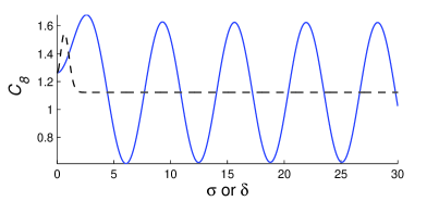
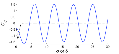
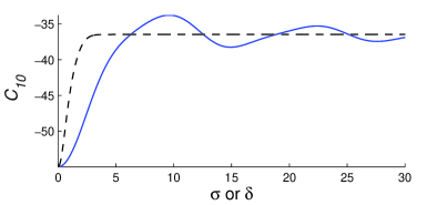
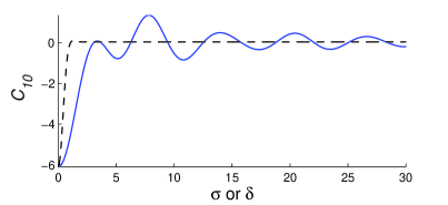
In the opposite limits, of wide kernels, where σ𝜎\sigma\rightarrow\infty in the Gaussian case, and δ𝛿\delta\rightarrow\infty in the top hat case, the coefficients again converge to the same values, although the convergence is oscillatory for the top hat kernel and monotonic for the Gaussian case.

5 Derivation of a cubic-quintic Ginzburg–Landau equation

In order to go beyond the solvability condition at O(ε3)𝑂superscript𝜀3O\left(\varepsilon^{3}\right) we need to incorporate higher-order contributions from the nonlocal term. This is a necessary preliminary to the investigation of the effects of the nonlocal term on the cubic-quintic Ginzburg–Landau equations near the codimension-two point at which the initial instability changes from supercritical to subcritical. In order to organise this calculation clearly, we first present our approach to the nonlocal term, before using these results in dealing order by order with the multiple scales computation.

5.1 Series expansion of the nonlocal term

In this section we develop an asymptotic expansion of the nonlocal term as a series in the envelope A(X)𝐴𝑋A(X) and its derivatives. The first term in this new expansion is the one that we have relied on in previous calculations. It turns out that we are able to derive a compact and general expression in terms of Fourier coefficients of the kernel: our expansion is therefore applicable to any kernel function that has a well defined, continuously differentiable Fourier transform.

The first step is to observe that all the integrals generated by the asymptotic analysis can be written in the general form

J=ΩK(xy)F[A(Y)]eimy𝑑y,𝐽subscriptΩ𝐾𝑥𝑦𝐹delimited-[]𝐴𝑌superscripte𝑖𝑚𝑦differential-d𝑦J=\int_{\Omega}K\left(x-y\right)F\left[A\left(Y\right)\right]\mathrm{e}^{imy}\,dy, (5.1)

where F𝐹F is a function of the amplitude A(X)𝐴𝑋A(X). We adopt the rescalings (2.8), i.e. X=ε2x𝑋superscript𝜀2𝑥X=\varepsilon^{2}x, and we consider the domain Ω=Ω\Omega=\mathbb{R}. We assume throughout that there are no technical difficulties with applying the Fourier transform. We use the following notation for the Fourier transform and its inverse:

[f(x)](k)f^(k)delimited-[]𝑓𝑥𝑘^𝑓𝑘\displaystyle\mathcal{F}\left[f\left(x\right)\right]\left(k\right)\equiv\hat{f}\left(k\right) :=assign\displaystyle:= f(x)eikx𝑑x,superscriptsubscript𝑓𝑥superscripte𝑖𝑘𝑥differential-d𝑥\displaystyle\int_{-\infty}^{\infty}f\left(x\right)\mathrm{e}^{-ikx}\ dx, (5.2)
1[f^(k)](x)f(x)superscript1delimited-[]^𝑓𝑘𝑥𝑓𝑥\displaystyle\mathbf{\mathcal{F}}^{-1}\left[\hat{f}\left(k\right)\right]\left(x\right)\equiv f\left(x\right) :=assign\displaystyle:= 12πf(k)eikx𝑑k.12𝜋superscriptsubscript𝑓𝑘superscripte𝑖𝑘𝑥differential-d𝑘\displaystyle\frac{1}{2\pi}\int_{-\infty}^{\infty}f\left(k\right)\mathrm{e}^{ikx}\ dk. (5.3)

We expand J𝐽J asymptotically in a series of straightforward steps which we now present. First, we make the substitution Y=ε2y𝑌superscript𝜀2𝑦Y=\varepsilon^{2}y in (5.1), and change the integration variable from y𝑦y to z=yx𝑧𝑦𝑥z=y-x to give

J=K(xy)F[A(Y)]eimy𝑑y=K(z)F[A(ε2x+ε2z)]eim(x+z)𝑑z.𝐽subscript𝐾𝑥𝑦𝐹delimited-[]𝐴𝑌superscripte𝑖𝑚𝑦differential-d𝑦subscript𝐾𝑧𝐹delimited-[]𝐴superscript𝜀2𝑥superscript𝜀2𝑧superscripte𝑖𝑚𝑥𝑧differential-d𝑧\displaystyle J=\int_{\mathbb{R}}K\left(x-y\right)F\left[A\left(Y\right)\right]\mathrm{e}^{imy}dy=\int_{\mathbb{R}}K\left(-z\right)F\left[A\left(\varepsilon^{2}x+\varepsilon^{2}z\right)\right]\mathrm{e}^{im\left(x+z\right)}\ dz.

Now we Taylor expand A(Y)𝐴𝑌A(Y) about the point X𝑋X, which gives

J𝐽\displaystyle J =\displaystyle= K(z)eim(x+z)n=0(ε2zDX)nn!F[A(X)]dz,subscript𝐾𝑧superscripte𝑖𝑚𝑥𝑧superscriptsubscript𝑛0superscriptsuperscript𝜀2𝑧subscript𝐷𝑋𝑛𝑛𝐹delimited-[]𝐴𝑋𝑑𝑧\displaystyle\int_{\mathbb{R}}K\left(-z\right)\mathrm{e}^{im\left(x+z\right)}\sum_{n=0}^{\infty}\frac{\left(\varepsilon^{2}zD_{X}\right)^{n}}{n!}F\left[A\left(X\right)\right]\ dz, (5.4)

where DXsubscript𝐷𝑋D_{X} stands for d/dX𝑑𝑑𝑋d/dX. Reversing the change of integration variable yields

J𝐽\displaystyle J =\displaystyle= K(xy)eimy[n=0(ε2DX)nn!F[A(X)](xy)n]𝑑y.subscript𝐾𝑥𝑦superscripte𝑖𝑚𝑦delimited-[]superscriptsubscript𝑛0superscriptsuperscript𝜀2subscript𝐷𝑋𝑛𝑛𝐹delimited-[]𝐴𝑋superscript𝑥𝑦𝑛differential-d𝑦\displaystyle\int_{\mathbb{R}}K\left(x-y\right)\mathrm{e}^{imy}\left[\sum_{n=0}^{\infty}\frac{\left(-\varepsilon^{2}D_{X}\right)^{n}}{n!}F\left[A\left(X\right)\right]\left(x-y\right)^{n}\right]\ dy.

We now take all the y𝑦y-independent terms outside the integral to obtain

J𝐽\displaystyle J =\displaystyle= n=0(ε2DX)nn!F[A(X)](xy)nK(xy)eimy𝑑y.superscriptsubscript𝑛0superscriptsuperscript𝜀2subscript𝐷𝑋𝑛𝑛𝐹delimited-[]𝐴𝑋subscriptsuperscript𝑥𝑦𝑛𝐾𝑥𝑦superscripte𝑖𝑚𝑦differential-d𝑦\displaystyle\sum_{n=0}^{\infty}\frac{\left(-\varepsilon^{2}D_{X}\right)^{n}}{n!}F\left[A\left(X\right)\right]\int_{\mathbb{R}}\left(x-y\right)^{n}K\left(x-y\right)\mathrm{e}^{imy}\ dy. (5.5)

The integral part of this expression is a convolution and so can be written (very compactly) in terms of Fourier transforms:

(xy)nK(xy)eimy𝑑ysuperscriptsubscriptsuperscript𝑥𝑦𝑛𝐾𝑥𝑦superscripte𝑖𝑚𝑦differential-d𝑦\displaystyle\int_{-\infty}^{\infty}\left(x-y\right)^{n}K\left(x-y\right)\mathrm{e}^{imy}dy =\displaystyle= 1[[xnK(x)][eimx]].superscript1delimited-[]delimited-[]superscript𝑥𝑛𝐾𝑥delimited-[]superscripte𝑖𝑚𝑥\displaystyle\mathcal{F^{\mathbf{\mathrm{-1}}}}\left[\mathcal{F}\left[x^{n}K\left(x\right)\right]\mathcal{F}\left[\mathrm{e}^{imx}\right]\right]. (5.6)

This expression can be simplified significantly further using the well-known Fourier transform properties that (i) the Fourier transform of a complex exponential is a Dirac delta function and and (ii) the effect of multiplication by a power of x𝑥x:

ei(mk)x𝑑x=2πδ(mk),andxnK(x)eikx𝑑x=(iDk)nK^(k).formulae-sequencesuperscriptsubscriptsuperscripte𝑖𝑚𝑘𝑥differential-d𝑥2𝜋𝛿𝑚𝑘andsuperscriptsubscriptsuperscript𝑥𝑛𝐾𝑥superscripte𝑖𝑘𝑥differential-d𝑥superscript𝑖subscript𝐷𝑘𝑛^𝐾𝑘\int_{-\infty}^{\infty}\mathrm{e}^{i\left(m-k\right)x}\ dx=2\pi\delta\left(m-k\right),\qquad\mathrm{and}\qquad\int_{-\infty}^{\infty}x^{n}K\left(x\right)\mathrm{e}^{-ikx}\ dx=\left(iD_{k}\right)^{n}\hat{K}\left(k\right). (5.7)

On substituting (5.7) into (5.6), we obtain

(xy)nK(xy)eimy𝑑ysuperscriptsubscriptsuperscript𝑥𝑦𝑛𝐾𝑥𝑦superscripte𝑖𝑚𝑦differential-d𝑦\displaystyle\int_{-\infty}^{\infty}\left(x-y\right)^{n}K\left(x-y\right)\mathrm{e}^{imy}dy =\displaystyle= 2π1[inDknK^δ(mk)]2𝜋superscript1delimited-[]superscript𝑖𝑛superscriptsubscript𝐷𝑘𝑛^𝐾𝛿𝑚𝑘\displaystyle 2\pi\mathcal{F^{\mathbf{\mathrm{-1}}}}\left[i^{n}D_{k}^{n}\hat{K}\ \delta\left(m-k\right)\right]
=\displaystyle= inDknK^δ(mk)eikx𝑑k=eimx(iDk)nK^(k)|k=msuperscriptsubscriptsuperscript𝑖𝑛superscriptsubscript𝐷𝑘𝑛^𝐾𝛿𝑚𝑘superscripte𝑖𝑘𝑥differential-d𝑘evaluated-atsuperscripte𝑖𝑚𝑥superscript𝑖subscript𝐷𝑘𝑛^𝐾𝑘𝑘𝑚\displaystyle\int_{-\infty}^{\infty}i^{n}D_{k}^{n}\hat{K}\ \delta\left(m-k\right)\mathrm{e}^{ikx}dk=\mathrm{e}^{imx}\left(iD_{k}\right)^{n}\left.\hat{K}\left(k\right)\right|_{k=m}

Returning to (5.5) we see that we have the expansion:

J=K(xy)F[A(Y)]eimy𝑑y=eimxn=0(iε2DXDk)nn!F[A(X)]K^(k)|k=m.𝐽subscript𝐾𝑥𝑦𝐹delimited-[]𝐴𝑌superscripte𝑖𝑚𝑦differential-d𝑦evaluated-atsuperscripte𝑖𝑚𝑥superscriptsubscript𝑛0superscript𝑖superscript𝜀2subscript𝐷𝑋subscript𝐷𝑘𝑛𝑛𝐹delimited-[]𝐴𝑋^𝐾𝑘𝑘𝑚\displaystyle J=\int_{\mathbb{R}}K\left(x-y\right)F\left[A\left(Y\right)\right]\mathrm{e}^{imy}dy=\mathrm{e}^{imx}\sum_{n=0}^{\infty}\frac{\left(-i\varepsilon^{2}D_{X}D_{k}\right)^{n}}{n!}F\left[A\left(X\right)\right]\left.\hat{K}\left(k\right)\right|_{k=m}. (5.8)

For use in the multiple scales analysis, it is convenient to collect the kernel-dependent parts of the expression into a set of coefficients Imnsubscript𝐼𝑚𝑛I_{mn} defined by

Imn:=(iDk)nK^(k)|k=m,assignsubscript𝐼𝑚𝑛evaluated-atsuperscript𝑖subscript𝐷𝑘𝑛^𝐾𝑘𝑘𝑚I_{mn}:=\left(-iD_{k}\right)^{n}\left.\hat{K}\left(k\right)\right|_{k=m}, (5.9)

which can then be evaluated at a later point, for a specific choice of kernel. Note that since we consider kernels that are even functions we have the relation Im0=I(m)0subscript𝐼𝑚0subscript𝐼𝑚0I_{m0}=I_{\left(-m\right)0}. In conclusion we have (formally) derived the series representation

K(xy)F[A(Y)]eimy𝑑y=eimxn=0Imn(ε2DX)nn!F[A(X)].superscriptsubscript𝐾𝑥𝑦𝐹delimited-[]𝐴𝑌superscripte𝑖𝑚𝑦differential-d𝑦superscripte𝑖𝑚𝑥superscriptsubscript𝑛0subscript𝐼𝑚𝑛superscriptsuperscript𝜀2subscript𝐷𝑋𝑛𝑛𝐹delimited-[]𝐴𝑋\displaystyle\int_{-\infty}^{\infty}K\left(x-y\right)F\left[A\left(Y\right)\right]\mathrm{e}^{imy}\ dy=\mathrm{e}^{imx}\sum_{n=0}^{\infty}I_{mn}\frac{\left(\varepsilon^{2}D_{X}\right)^{n}}{n!}F\left[A\left(X\right)\right]. (5.10)

5.2 Asymptotic expansion

Having found a general expansion for the integrals arising in the multiple scales analysis, it is now possible to carry out the derivation of a cubic-quintic Ginzburg–Landau equation where the nonlocal term is included, using the alternative scalings (2.8) and the expansion (2.2). Previously, under the O(ε3)𝑂superscript𝜀3O(\varepsilon^{3}) scalings, the nonlocal term was found to introduce a width dependency into the coefficient of the A|A|2𝐴superscript𝐴2A\left|A\right|^{2} term. Using the more complicated scalings, it is now shown that similar dependencies appear in the higher order A|A|4𝐴superscript𝐴4A\left|A\right|^{4} term. As stated, we leave the kernel dependent coefficients Imnsubscript𝐼𝑚𝑛I_{mn} unevaluated in the derivation and later generate appropriate values for both top hat and Gaussian kernels through equation (5.9).

The procedure for generating the relevant PDE for A𝐴A through the multiple scales analysis is much the same as that discussed for the local problem in section 2.3. As there are no integral terms at O(ε)𝑂𝜀O\left(\varepsilon\right) the ansatz for u1subscript𝑢1u_{1} remains unchanged, as do the scalings for X𝑋X,T𝑇T and μ𝜇\mu. However, with the addition of the nonlocal term the codimension-two point in the N23subscript𝑁23N_{23} equation is no longer b=2738𝑏2738b=\sqrt{\frac{27}{38}} and the parameter b𝑏b must instead be expanded about the point

b0=2738+9γ38(2I00+I20),subscript𝑏027389𝛾382subscript𝐼00subscript𝐼20b_{0}=\sqrt{\frac{27}{38}+\frac{9\gamma}{38}\left(2I_{00}+I_{20}\right)}, (5.11)

which depends on the form of (the Fourier transform of) the kernel K(x)𝐾𝑥K(x). Explicitly we write

b=b0+ε2b2.𝑏subscript𝑏0superscript𝜀2subscript𝑏2b=b_{0}+\varepsilon^{2}b_{2}. (5.12)

We remark, for reference, that the codimension two point defined by r=0𝑟0r=0 and b=b0𝑏subscript𝑏0b=b_{0}, given by (5.11), corresponds to the codimension-two case of the bifurcation problem in the spatial dynamics setting studied by Woods and Champneys [29]. In that paper the condition b=b0𝑏subscript𝑏0b=b_{0} is the condition q2=0subscript𝑞20q_{2}=0 where q2subscript𝑞2q_{2} is one of the crucial normal form coefficients for determining the qualitative behaviour of solutions near the bifurcation point.

5.3 Detailed derivation of the cubic–quintic amplitude equation

We now present the derivation of the cubic-quintic amplitude equation in detail in order to show exactly how we make (repeated) use of the series expansion (5.10). For clarity, we restate the nonlocal (2–3) Swift–Hohenberg equation (3.1).

tu=[r(1+x2)2]u+bu2u3γu(x,t)ΩK(xy)u(y,t)2𝑑y.subscript𝑡𝑢delimited-[]𝑟superscript1superscriptsubscript𝑥22𝑢𝑏superscript𝑢2superscript𝑢3𝛾𝑢𝑥𝑡subscriptΩ𝐾𝑥𝑦𝑢superscript𝑦𝑡2differential-d𝑦\partial_{t}u=\left[r-\left(1+\partial_{x}^{2}\right)^{2}\right]u+bu^{2}-u^{3}-\gamma u(x,t)\int_{\Omega}K\left(x-y\right)u(y,t)^{2}dy.

We expand as usual in an asymptotic series:

u(x,X,t,T)=εu1+ε2u2+ε3u3+ε4u4+ε5u5+,𝑢𝑥𝑋𝑡𝑇𝜀subscript𝑢1superscript𝜀2subscript𝑢2superscript𝜀3subscript𝑢3superscript𝜀4subscript𝑢4superscript𝜀5subscript𝑢5u\left(x,X,t,T\right)=\varepsilon u_{1}+\varepsilon^{2}u_{2}+\varepsilon^{3}u_{3}+\varepsilon^{4}u_{4}+\varepsilon^{5}u_{5}+\cdots,

and solve order by order in ε𝜀\varepsilon until we obtain a non-trivial solvability condition. To simplify notation we define the linear operator

[u]:=(1+x2)2u.assigndelimited-[]𝑢superscript1superscriptsubscript𝑥22𝑢\displaystyle\mathcal{L}[u]:=-(1+\partial_{x}^{2})^{2}u.

Terms at O(ε)𝑂𝜀O\left(\varepsilon\right) and O(ε2)𝑂superscript𝜀2O\left(\varepsilon^{2}\right).

Since the nonlocal term is cubic in u𝑢u, it does not affect the forms of u1subscript𝑢1u_{1} and u2subscript𝑢2u_{2}. Solving at O(ε)𝑂𝜀O\left(\varepsilon\right) and O(ε2)𝑂superscript𝜀2O\left(\varepsilon^{2}\right) and using (5.12) we obtain the expected expressions

u1(x,X,t,T)=A(X,T)eix+A¯(X,T)eix,subscript𝑢1𝑥𝑋𝑡𝑇𝐴𝑋𝑇superscripte𝑖𝑥¯𝐴𝑋𝑇superscripte𝑖𝑥u_{1}\left(x,X,t,T\right)=A\left(X,T\right)\mathrm{e}^{ix}+\bar{A}\left(X,T\right)\mathrm{e}^{-ix},

and

u2=b0(2|A|2+19A2e2ix+19A¯2e2ix).subscript𝑢2subscript𝑏02superscript𝐴219superscript𝐴2superscripte2𝑖𝑥19superscript¯𝐴2superscripte2𝑖𝑥u_{2}=b_{0}\left(2\left|A\right|^{2}+\frac{1}{9}A^{2}\mathrm{e}^{2ix}+\frac{1}{9}\bar{A}^{2}\mathrm{e}^{-2ix}\right). (5.13)

Terms at O(ε3)𝑂superscript𝜀3O(\varepsilon^{3}).

O(ε3)𝑂superscript𝜀3O(\varepsilon^{3}) is the lowest order at which a term from the nonlocal expression enters directly. We have

tu3subscript𝑡subscript𝑢3\displaystyle\partial_{t}u_{3} =\displaystyle= [u3]4xX(1+x2)u1=0+2b0u1u2u13γu1ΩK(xy)u12(y)𝑑y,delimited-[]subscript𝑢34subscript𝑥subscript𝑋subscript1superscriptsubscript𝑥2subscript𝑢1absent02subscript𝑏0subscript𝑢1subscript𝑢2superscriptsubscript𝑢13𝛾subscript𝑢1subscriptΩ𝐾𝑥𝑦superscriptsubscript𝑢12𝑦differential-d𝑦\displaystyle\mathcal{L}\left[u_{3}\right]-4\partial_{x}\partial_{X}\underbrace{\left(1+\partial_{x}^{2}\right)u_{1}}_{=0}+2b_{0}u_{1}u_{2}-u_{1}^{3}-\gamma u_{1}\int_{\Omega}K\left(x-y\right)u_{1}^{2}\left(y\right)dy, (5.14)

and so to find u3subscript𝑢3u_{3} we need to solve

[u3]+2b0u1u2u13γu1ΩK(xy)u12(y)𝑑y=0.delimited-[]subscript𝑢32subscript𝑏0subscript𝑢1subscript𝑢2superscriptsubscript𝑢13𝛾subscript𝑢1subscriptΩ𝐾𝑥𝑦superscriptsubscript𝑢12𝑦differential-d𝑦0\displaystyle\mathcal{L}[u_{3}]+2b_{0}u_{1}u_{2}-u_{1}^{3}-\gamma u_{1}\int_{\Omega}K\left(x-y\right)u_{1}^{2}\left(y\right)dy=0.

We expand the integral operator by using the series expansion (5.10), noting that all terms in the expansion where n>0𝑛0n>0 contribute at least an additional factor of ε2superscript𝜀2\varepsilon^{2} and hence only the leading order term in J11subscript𝐽11J_{11} contributes at this order:

J11ΩK(xy)u12(y)𝑑ysubscript𝐽11subscriptΩ𝐾𝑥𝑦superscriptsubscript𝑢12𝑦differential-d𝑦\displaystyle J_{11}\equiv\int_{\Omega}K(x-y)u_{1}^{2}\left(y\right)dy =\displaystyle= J11(0)+ε2J11(2)+O(ε4)superscriptsubscript𝐽110superscript𝜀2superscriptsubscript𝐽112𝑂superscript𝜀4\displaystyle J_{11}^{(0)}+\varepsilon^{2}J_{11}^{(2)}+O(\varepsilon^{4})
=\displaystyle= 2|A|2I00+I20(A2e2ix+A¯2e2ix)+O(ε2).2superscript𝐴2subscript𝐼00subscript𝐼20superscript𝐴2superscripte2𝑖𝑥superscript¯𝐴2superscripte2𝑖𝑥𝑂superscript𝜀2\displaystyle 2\left|A\right|^{2}I_{00}+I_{20}\left(A^{2}\mathrm{e}^{2ix}+\bar{A}^{2}\mathrm{e}^{-2ix}\right)+O(\varepsilon^{2}).

At this order we ignore J11(2)superscriptsubscript𝐽112J_{11}^{(2)}, and, after multiplying by γu1𝛾subscript𝑢1\gamma u_{1} we obtain

γu1ΩK(xy)u12(y)𝑑y=γ[eix(2I00+I20)A|A|2+e3ixI20A3]+c.c.+O(ε2)formulae-sequence𝛾subscript𝑢1subscriptΩ𝐾𝑥𝑦superscriptsubscript𝑢12𝑦differential-d𝑦𝛾delimited-[]superscripte𝑖𝑥2subscript𝐼00subscript𝐼20𝐴superscript𝐴2superscripte3𝑖𝑥subscript𝐼20superscript𝐴3𝑐𝑐𝑂superscript𝜀2\gamma u_{1}\int_{\Omega}K\left(x-y\right)u_{1}^{2}\left(y\right)dy=\gamma\left[\mathrm{e}^{ix}\left(2I_{00}+I_{20}\right)A\left|A\right|^{2}+\mathrm{e}^{3ix}I_{20}A^{3}\right]+c.c.+O(\varepsilon^{2}) (5.16)

The remaining (local) nonlinear terms in (5.14) are

2b0u1u2u132subscript𝑏0subscript𝑢1subscript𝑢2superscriptsubscript𝑢13\displaystyle 2b_{0}u_{1}u_{2}-u_{1}^{3} =\displaystyle= 29b02(A3e3ix+A¯3e3ix+19A|A|2eix+19A¯|A|2eix)29superscriptsubscript𝑏02superscript𝐴3superscripte3𝑖𝑥superscript¯𝐴3superscripte3𝑖𝑥19𝐴superscript𝐴2superscripte𝑖𝑥19¯𝐴superscript𝐴2superscripte𝑖𝑥\displaystyle\frac{2}{9}b_{0}^{2}\left(A^{3}\mathrm{e}^{3ix}+\bar{A}^{3}\mathrm{e}^{-3ix}+19A\left|A\right|^{2}\mathrm{e}^{ix}+19\bar{A}\left|A\right|^{2}\mathrm{e}^{-ix}\right) (5.17)
(A3e3ix+3A|A|2eix+3A¯|A|2eix+A¯3e3ix)superscript𝐴3superscripte3𝑖𝑥3𝐴superscript𝐴2superscripte𝑖𝑥3¯𝐴superscript𝐴2superscripte𝑖𝑥superscript¯𝐴3superscripte3𝑖𝑥\displaystyle-\left(A^{3}\mathrm{e}^{3ix}+3A\left|A\right|^{2}\mathrm{e}^{ix}+3\bar{A}\left|A\right|^{2}\mathrm{e}^{-ix}+\bar{A}^{3}\mathrm{e}^{-3ix}\right)
=\displaystyle= eix(389b023)A|A|2+e3ix(29b021)A3+c.c.formulae-sequencesuperscripte𝑖𝑥389superscriptsubscript𝑏023𝐴superscript𝐴2superscripte3𝑖𝑥29superscriptsubscript𝑏021superscript𝐴3𝑐𝑐\displaystyle\mathrm{e}^{ix}\left(\frac{38}{9}b_{0}^{2}-3\right)A\left|A\right|^{2}+\mathrm{e}^{3ix}\left(\frac{2}{9}b_{0}^{2}-1\right)A^{3}+c.c.

Combining (5.16) and (5.17) we have

2b0u1u2u13γu1ΩK(xy)u12(y)𝑑y2subscript𝑏0subscript𝑢1subscript𝑢2superscriptsubscript𝑢13𝛾subscript𝑢1subscriptΩ𝐾𝑥𝑦superscriptsubscript𝑢12𝑦differential-d𝑦\displaystyle 2b_{0}u_{1}u_{2}-u_{1}^{3}-\gamma u_{1}\int_{\Omega}K\left(x-y\right)u_{1}^{2}\left(y\right)dy =\displaystyle= eix(389b023γ(2I00+I20))A|A|2superscripte𝑖𝑥389superscriptsubscript𝑏023𝛾2subscript𝐼00subscript𝐼20𝐴superscript𝐴2\displaystyle\mathrm{e}^{ix}\left(\frac{38}{9}b_{0}^{2}-3-\gamma\left(2I_{00}+I_{20}\right)\right)A\left|A\right|^{2}
+e3ix(29b021γI20)A3+c.c..formulae-sequencesuperscripte3𝑖𝑥29superscriptsubscript𝑏021𝛾subscript𝐼20superscript𝐴3𝑐𝑐\displaystyle+\mathrm{e}^{3ix}\left(\frac{2}{9}b_{0}^{2}-1-\gamma I_{20}\right)A^{3}+c.c..

The definition (5.11) of b0subscript𝑏0b_{0} shows that the coefficients of e±ixsuperscripteplus-or-minus𝑖𝑥\mathrm{e}^{\pm ix} vanish, and that the coefficient of e3ixsuperscripte3𝑖𝑥\mathrm{e}^{3ix} can be simplified:

29b021γI2029superscriptsubscript𝑏021𝛾subscript𝐼20\displaystyle\frac{2}{9}b_{0}^{2}-1-\gamma I_{20} =\displaystyle= 29(2738+9γ38(2I00+I20))1γI20=1619+2γ19(I009I20).2927389𝛾382subscript𝐼00subscript𝐼201𝛾subscript𝐼2016192𝛾19subscript𝐼009subscript𝐼20\displaystyle\frac{2}{9}\left(\frac{27}{38}+\frac{9\gamma}{38}\left(2I_{00}+I_{20}\right)\right)-1-\gamma I_{20}=-\frac{16}{19}+\frac{2\gamma}{19}\left(I_{00}-9I_{20}\right).

We therefore obtain a solution for u3subscript𝑢3u_{3} in the form

u3=C2(A3e3ix+A¯3e3ix),whereC2=176+γ608(I009I20).formulae-sequencesubscript𝑢3subscript𝐶2superscript𝐴3superscripte3𝑖𝑥superscript¯𝐴3superscripte3𝑖𝑥wheresubscript𝐶2176𝛾608subscript𝐼009subscript𝐼20\displaystyle u_{3}=C_{2}\left(A^{3}\mathrm{e}^{3ix}+\bar{A}^{3}\mathrm{e}^{-3ix}\right),\qquad\mathrm{where}\qquad C_{2}=-\frac{1}{76}+\frac{\gamma}{608}\left(I_{00}-9I_{20}\right).

Terms at O(ε4)𝑂superscript𝜀4O(\varepsilon^{4}).

At fourth order in ε𝜀\varepsilon we obtain

tu4subscript𝑡subscript𝑢4\displaystyle\partial_{t}u_{4} =\displaystyle= [u4]4xX(1+x2)u2+b2u12+b0(u22+2u1u3)3u12u2delimited-[]subscript𝑢44subscript𝑥subscript𝑋1superscriptsubscript𝑥2subscript𝑢2subscript𝑏2superscriptsubscript𝑢12subscript𝑏0superscriptsubscript𝑢222subscript𝑢1subscript𝑢33superscriptsubscript𝑢12subscript𝑢2\displaystyle\mathcal{L}\left[u_{4}\right]-4\partial_{x}\partial_{X}\left(1+\partial_{x}^{2}\right)u_{2}+b_{2}u_{1}^{2}+b_{0}\left(u_{2}^{2}+2u_{1}u_{3}\right)-3u_{1}^{2}u_{2} (5.18)
γu2ΩK(xy)u12(y)𝑑y2γu1ΩK(xy)u1(y)u2(y)𝑑y𝛾subscript𝑢2subscriptΩ𝐾𝑥𝑦superscriptsubscript𝑢12𝑦differential-d𝑦2𝛾subscript𝑢1subscriptΩ𝐾𝑥𝑦subscript𝑢1𝑦subscript𝑢2𝑦differential-d𝑦\displaystyle-\gamma u_{2}\int_{\Omega}K\left(x-y\right)u_{1}^{2}\left(y\right)dy-2\gamma u_{1}\int_{\Omega}K\left(x-y\right)u_{1}\left(y\right)u_{2}\left(y\right)dy

which includes contributions from two integral terms: J11subscript𝐽11J_{11} and J12subscript𝐽12J_{12}. We write this schematically in the form

tu4subscript𝑡subscript𝑢4\displaystyle\partial_{t}u_{4} =\displaystyle= [u4]+f4L+f4NL,delimited-[]subscript𝑢4subscript𝑓4𝐿subscript𝑓4𝑁𝐿\displaystyle\mathcal{L}\left[u_{4}\right]+f_{4L}+f_{4NL},

collecting the local and integral terms into f4Lsubscript𝑓4𝐿f_{4L} and f4NLsubscript𝑓4𝑁𝐿f_{4NL} respectively so that we can consider them separately in what follows.

Local terms at O(ε4)𝑂superscript𝜀4O(\varepsilon^{4}).

Expanding the four local terms we obtain:

4xX(1+x2)u24subscript𝑥subscript𝑋1superscriptsubscript𝑥2subscript𝑢2\displaystyle-4\partial_{x}\partial_{X}\left(1+\partial_{x}^{2}\right)u_{2} =\displaystyle= 16i3b0(AAXe2ixA¯A¯Xe2ix),16𝑖3subscript𝑏0𝐴subscript𝐴𝑋superscripte2𝑖𝑥¯𝐴subscript¯𝐴𝑋superscripte2𝑖𝑥\displaystyle\frac{16i}{3}b_{0}\left(AA_{X}\mathrm{e}^{2ix}-\bar{A}\bar{A}_{X}\mathrm{e}^{-2ix}\right),
b2u12subscript𝑏2superscriptsubscript𝑢12\displaystyle b_{2}u_{1}^{2} =\displaystyle= b2(2|A|2+A2e2ix+A¯2e2ix),subscript𝑏22superscript𝐴2superscript𝐴2superscripte2𝑖𝑥superscript¯𝐴2superscripte2𝑖𝑥\displaystyle b_{2}\left(2\left|A\right|^{2}+A^{2}\mathrm{e}^{2ix}+\bar{A}^{2}\mathrm{e}^{-2ix}\right),
b0(u22+2u1u3)subscript𝑏0superscriptsubscript𝑢222subscript𝑢1subscript𝑢3\displaystyle b_{0}\left(u_{2}^{2}+2u_{1}u_{3}\right) =\displaystyle= 32681b03|A|4+e2ix(49b03+2b0C2)A2|A|232681superscriptsubscript𝑏03superscript𝐴4superscripte2𝑖𝑥49superscriptsubscript𝑏032subscript𝑏0subscript𝐶2superscript𝐴2superscript𝐴2\displaystyle\frac{326}{81}b_{0}^{3}\left|A\right|^{4}+\mathrm{e}^{2ix}\left(\frac{4}{9}b_{0}^{3}+2b_{0}C_{2}\right)A^{2}\left|A\right|^{2}
+e4ix(b0381+2b0C2)A4+c.c.,formulae-sequencesuperscripte4𝑖𝑥superscriptsubscript𝑏03812subscript𝑏0subscript𝐶2superscript𝐴4𝑐𝑐\displaystyle+\mathrm{e}^{4ix}\left(\frac{b_{0}^{3}}{81}+2b_{0}C_{2}\right)A^{4}+c.c.,
3u12u23superscriptsubscript𝑢12subscript𝑢2\displaystyle-3u_{1}^{2}u_{2} =\displaystyle= 383b0|A|4e2ix203b0A2|A|2e4ix13C1A4c.c..formulae-sequence383subscript𝑏0superscript𝐴4superscripte2𝑖𝑥203subscript𝑏0superscript𝐴2superscript𝐴2superscripte4𝑖𝑥13subscript𝐶1superscript𝐴4𝑐𝑐\displaystyle-\frac{38}{3}b_{0}\left|A\right|^{4}-\mathrm{e}^{2ix}\frac{20}{3}b_{0}A^{2}\left|A\right|^{2}-\mathrm{e}^{4ix}\frac{1}{3}C_{1}A^{4}-c.c..

Collecting together all these terms we obtain

f4Lsubscript𝑓4𝐿\displaystyle f_{4L} =\displaystyle= 16i3b0(AAXe2ixA¯A¯Xe2ix)+2b3|A|2+b3A2e2ix16𝑖3subscript𝑏0𝐴subscript𝐴𝑋superscripte2𝑖𝑥¯𝐴subscript¯𝐴𝑋superscripte2𝑖𝑥2subscript𝑏3superscript𝐴2subscript𝑏3superscript𝐴2superscripte2𝑖𝑥\displaystyle\frac{16i}{3}b_{0}\left(AA_{X}\mathrm{e}^{2ix}-\bar{A}\bar{A}_{X}\mathrm{e}^{-2ix}\right)+2b_{3}\left|A\right|^{2}+b_{3}A^{2}\mathrm{e}^{2ix}
+(32681b03383b0)|A|4+e2ix(49b03+2b0C2609b0)A2|A|232681superscriptsubscript𝑏03383subscript𝑏0superscript𝐴4superscripte2𝑖𝑥49superscriptsubscript𝑏032subscript𝑏0subscript𝐶2609subscript𝑏0superscript𝐴2superscript𝐴2\displaystyle+\left(\frac{326}{81}b_{0}^{3}-\frac{38}{3}b_{0}\right)\left|A\right|^{4}+\mathrm{e}^{2ix}\left(\frac{4}{9}b_{0}^{3}+2b_{0}C_{2}-\frac{60}{9}b_{0}\right)A^{2}\left|A\right|^{2}
+e4ix(b0381+2b0C2b03)A4+c.c..formulae-sequencesuperscripte4𝑖𝑥superscriptsubscript𝑏03812subscript𝑏0subscript𝐶2subscript𝑏03superscript𝐴4𝑐𝑐\displaystyle+\mathrm{e}^{4ix}\left(\frac{b_{0}^{3}}{81}+2b_{0}C_{2}-\frac{b_{0}}{3}\right)A^{4}+c.c.\ .

Integral terms at O(ε4)𝑂superscript𝜀4O(\varepsilon^{4}).

We now turn to the nonlocal terms. Using the series expansions, the two integral terms are evaluated to give the following:

J11ΩK(xy)u12(y)𝑑ysubscript𝐽11subscriptΩ𝐾𝑥𝑦superscriptsubscript𝑢12𝑦differential-d𝑦\displaystyle J_{11}\equiv\int_{\Omega}K\left(x-y\right)u_{1}^{2}\left(y\right)dy =\displaystyle= 2|A|2I00+I20(A2e2ix+A¯2e2ix),2superscript𝐴2subscript𝐼00subscript𝐼20superscript𝐴2superscript𝑒2𝑖𝑥superscript¯𝐴2superscript𝑒2𝑖𝑥\displaystyle 2\left|A\right|^{2}I_{00}+I_{20}\left(A^{2}e^{2ix}+\bar{A}^{2}e^{-2ix}\right),
J12ΩK(xy)u1(y)u2(y)𝑑ysubscript𝐽12subscriptΩ𝐾𝑥𝑦subscript𝑢1𝑦subscript𝑢2𝑦differential-d𝑦\displaystyle J_{12}\equiv\int_{\Omega}K\left(x-y\right)u_{1}\left(y\right)u_{2}\left(y\right)dy =\displaystyle= b09[19I10(A|A|2eix+A¯|A|2eix)\displaystyle\frac{b_{0}}{9}\left[19I_{10}(A\left|A\right|^{2}e^{ix}+\bar{A}\left|A\right|^{2}e^{-ix})\right.
+I30(A3e3ix+A¯3e3ix)],\displaystyle\left.+I_{30}(A^{3}e^{3ix}+\bar{A}^{3}e^{-3ix})\right],

ignoring higher-order contributions in ε𝜀\varepsilon. The nonlocal terms can then be evaluated to give

γu2ΩK(xy)u12(y)𝑑y𝛾subscript𝑢2subscriptΩ𝐾𝑥𝑦superscriptsubscript𝑢12𝑦differential-d𝑦\displaystyle\gamma u_{2}\int_{\Omega}K\left(x-y\right)u_{1}^{2}\left(y\right)dy =\displaystyle= γb0[(4I00+29I20)|A|4+e2ix(2I20+29I00)A2|A|2\displaystyle\gamma b_{0}\left[\left(4I_{00}+\frac{2}{9}I_{20}\right)\left|A\right|^{4}+\mathrm{e}^{2ix}\left(2I_{20}+\frac{2}{9}I_{00}\right)A^{2}\left|A\right|^{2}\right.
+I209A4e4ix]+c.c.,\displaystyle\left.+\frac{I_{20}}{9}A^{4}\mathrm{e}^{4ix}\right]+c.c.,

and

2γu1ΩK(xy)u1(y)u2(y)𝑑y2𝛾subscript𝑢1subscriptΩ𝐾𝑥𝑦subscript𝑢1𝑦subscript𝑢2𝑦differential-d𝑦\displaystyle 2\gamma u_{1}\int_{\Omega}K\left(x-y\right)u_{1}\left(y\right)u_{2}\left(y\right)dy =\displaystyle= 29γb0[38I10|A|4+e2ix(19I10+I30)A2|A|2\displaystyle\frac{2}{9}\gamma b_{0}\left[38I_{10}\left|A\right|^{4}+\mathrm{e}^{2ix}\left(19I_{10}+I_{30}\right)A^{2}\left|A\right|^{2}\right.
+I30A4e4ix]+c.c..\displaystyle\left.+I_{30}A^{4}\mathrm{e}^{4ix}\right]+c.c.\ .

These contributions to the right hand side of (5.18) can be collected together to give

f4NLsubscript𝑓4𝑁𝐿\displaystyle f_{4NL} =\displaystyle= γb09[(36I00+76I10+2I20)|A|4+e2ix(2I00+38I10+18I20+2I30)A2|A|2\displaystyle\frac{\gamma b_{0}}{9}\left[\left(36I_{00}+76I_{10}+2I_{20}\right)\left|A\right|^{4}+\mathrm{e}^{2ix}\left(2I_{00}+38I_{10}+18I_{20}+2I_{30}\right)A^{2}\left|A\right|^{2}\right.
+e4ix(I20+2I30)A4]+c.c.\displaystyle\left.+\mathrm{e}^{4ix}\left(I_{20}+2I_{30}\right)A^{4}\right]+c.c.

Solution at O(ε4)𝑂superscript𝜀4O(\varepsilon^{4}).

The equation for u4subscript𝑢4u_{4} therefore reduces to

0=[u4]+2b3|A|2+C3|A|4+(i163C1AAX+b3A2+C4A2|A|2)e2ix+C5A4e4ix+c.c.formulae-sequence0delimited-[]subscript𝑢42subscript𝑏3superscript𝐴2subscript𝐶3superscript𝐴4𝑖163subscript𝐶1𝐴subscript𝐴𝑋subscript𝑏3superscript𝐴2subscript𝐶4superscript𝐴2superscript𝐴2superscripte2𝑖𝑥subscript𝐶5superscript𝐴4superscripte4𝑖𝑥𝑐𝑐\displaystyle 0=\mathcal{L}\left[u_{4}\right]+2b_{3}\left|A\right|^{2}+C_{3}\left|A\right|^{4}+\left(i\frac{16}{3}C_{1}AA_{X}+b_{3}A^{2}+C_{4}A^{2}\left|A\right|^{2}\right)\mathrm{e}^{2ix}+C_{5}A^{4}\mathrm{e}^{4ix}+c.c.
(5.19)

where we have defined the constants C3subscript𝐶3C_{3}, C4subscript𝐶4C_{4} and C5subscript𝐶5C_{5} to be

C3subscript𝐶3\displaystyle C_{3} =\displaystyle= b0[32681b023832γ(2I00+389I10+19I20)],subscript𝑏0delimited-[]32681superscriptsubscript𝑏023832𝛾2subscript𝐼00389subscript𝐼1019subscript𝐼20\displaystyle b_{0}\left[\frac{326}{81}b_{0}^{2}-\frac{38}{3}-2\gamma\left(2I_{00}+\frac{38}{9}I_{10}+\frac{1}{9}I_{20}\right)\right],
C4subscript𝐶4\displaystyle C_{4} =\displaystyle= b0[49b02+2C22032γ9(I00+19I10+9I20+I30)],subscript𝑏0delimited-[]49superscriptsubscript𝑏022subscript𝐶22032𝛾9subscript𝐼0019subscript𝐼109subscript𝐼20subscript𝐼30\displaystyle b_{0}\left[\frac{4}{9}b_{0}^{2}+2C_{2}-\frac{20}{3}-\frac{2\gamma}{9}\left(I_{00}+19I_{10}+9I_{20}+I_{30}\right)\right],
C5subscript𝐶5\displaystyle C_{5} =\displaystyle= b0[b0281+2C213γ9(I20+2I30)].subscript𝑏0delimited-[]superscriptsubscript𝑏02812subscript𝐶213𝛾9subscript𝐼202subscript𝐼30\displaystyle b_{0}\left[\frac{b_{0}^{2}}{81}+2C_{2}-\frac{1}{3}-\frac{\gamma}{9}\left(I_{20}+2I_{30}\right)\right].

Equation (5.19) can be solved straightforwardly, since there are no terms in e±ixsuperscripteplus-or-minus𝑖𝑥\mathrm{e}^{\pm ix}, by acting with 1superscript1\mathcal{L}^{-1}. We therefore obtain the solution

u4=2b3|A|2+C3|A|4+(i1627C1AAX+b39A2+C49A2|A|2)e2ix+C5225A4e4ix+c.c..formulae-sequencesubscript𝑢42subscript𝑏3superscript𝐴2subscript𝐶3superscript𝐴4𝑖1627subscript𝐶1𝐴subscript𝐴𝑋subscript𝑏39superscript𝐴2subscript𝐶49superscript𝐴2superscript𝐴2superscripte2𝑖𝑥subscript𝐶5225superscript𝐴4superscripte4𝑖𝑥𝑐𝑐u_{4}=2b_{3}\left|A\right|^{2}+C_{3}\left|A\right|^{4}+\left(i\frac{16}{27}C_{1}AA_{X}+\frac{b_{3}}{9}A^{2}+\frac{C_{4}}{9}A^{2}\left|A\right|^{2}\right)\mathrm{e}^{2ix}+\frac{C_{5}}{225}A^{4}\mathrm{e}^{4ix}+c.c.\ .

Terms at O(ε5)𝑂superscript𝜀5O(\varepsilon^{5}).

Continuing to fifth order in ε𝜀\varepsilon we pick up contributions from three additional integral terms as well as higher-order contributions from J11subscript𝐽11J_{11} - recall that at O(ε3)𝑂superscript𝜀3O(\varepsilon^{3}) we considered only the leading order part of J11subscript𝐽11J_{11}. At O(ε5)𝑂superscript𝜀5O(\varepsilon^{5}) we seek only to identify the coefficients of the e±ixsuperscripteplus-or-minus𝑖𝑥\mathrm{e}^{\pm ix} terms in order to deduce a solvability condition; we do not need to solve completely for u5subscript𝑢5u_{5}. Considering terms at O(ε5)𝑂superscript𝜀5O(\varepsilon^{5}) in (3.1) we have

tu5+Tu1subscript𝑡subscript𝑢5subscript𝑇subscript𝑢1\displaystyle\partial_{t}u_{5}+\partial_{T}u_{1} =\displaystyle= [u5]+(μ+4X2)u14xX(1+x2)u3+2b2u1u2+2b0(u2u3+u1u4)delimited-[]subscript𝑢5𝜇4superscriptsubscript𝑋2subscript𝑢14subscript𝑥subscript𝑋1superscriptsubscript𝑥2subscript𝑢32subscript𝑏2subscript𝑢1subscript𝑢22subscript𝑏0subscript𝑢2subscript𝑢3subscript𝑢1subscript𝑢4\displaystyle\mathcal{L}\left[u_{5}\right]+\left(\mu+4\partial_{X}^{2}\right)u_{1}-4\partial_{x}\partial_{X}\left(1+\partial_{x}^{2}\right)u_{3}+2b_{2}u_{1}u_{2}+2b_{0}\left(u_{2}u_{3}+u_{1}u_{4}\right)
3(u1u22+u12u3)γu3ΩK(xy)u12(y)𝑑y3subscript𝑢1superscriptsubscript𝑢22superscriptsubscript𝑢12subscript𝑢3𝛾subscript𝑢3subscriptΩ𝐾𝑥𝑦superscriptsubscript𝑢12𝑦differential-d𝑦\displaystyle-3\left(u_{1}u_{2}^{2}+u_{1}^{2}u_{3}\right)-\gamma u_{3}\int_{\Omega}K\left(x-y\right)u_{1}^{2}\left(y\right)dy
2γu2ΩK(xy)u1(y)u2(y)𝑑y2𝛾subscript𝑢2subscriptΩ𝐾𝑥𝑦subscript𝑢1𝑦subscript𝑢2𝑦differential-d𝑦\displaystyle-2\gamma u_{2}\int_{\Omega}K\left(x-y\right)u_{1}\left(y\right)u_{2}\left(y\right)dy
γu1ΩK(xy)(2u1(y)u3(y)+u22(y))𝑑y,𝛾subscript𝑢1subscriptΩ𝐾𝑥𝑦2subscript𝑢1𝑦subscript𝑢3𝑦superscriptsubscript𝑢22𝑦differential-d𝑦\displaystyle-\gamma u_{1}\int_{\Omega}K\left(x-y\right)\left(2u_{1}\left(y\right)u_{3}\left(y\right)+u_{2}^{2}\left(y\right)\right)dy,
=\displaystyle= [u5]+f5L+f5NL.delimited-[]subscript𝑢5subscript𝑓5𝐿subscript𝑓5𝑁𝐿\displaystyle\mathcal{L}\left[u_{5}\right]+f_{5L}+f_{5NL}.

Local terms at O(ε5)𝑂superscript𝜀5O(\varepsilon^{5}).

The local terms in (5.3) contribute the following terms that contain a factor of eixsuperscripte𝑖𝑥\mathrm{e}^{ix} (we list only those terms, and ignore terms containing factors of eiqxsuperscripte𝑖𝑞𝑥\mathrm{e}^{iqx} where q1𝑞1q\neq 1):

(μ+4X2)u1𝜇4superscriptsubscript𝑋2subscript𝑢1\displaystyle\left(\mu+4\partial_{X}^{2}\right)u_{1} =\displaystyle= (μA+4AXX)eix+,𝜇𝐴4subscript𝐴𝑋𝑋superscripte𝑖𝑥\displaystyle\left(\mu A+4A_{XX}\right)\mathrm{e}^{ix}+\cdots,
2b2u1u22subscript𝑏2subscript𝑢1subscript𝑢2\displaystyle 2b_{2}u_{1}u_{2} =\displaystyle= 389b2b0A|A|2eix+,389subscript𝑏2subscript𝑏0𝐴superscript𝐴2superscripte𝑖𝑥\displaystyle\frac{38}{9}b_{2}b_{0}A\left|A\right|^{2}\mathrm{e}^{ix}+\cdots,
2b0u2u32subscript𝑏0subscript𝑢2subscript𝑢3\displaystyle 2b_{0}u_{2}u_{3} =\displaystyle= 29b02C2A|A|4eix+,29superscriptsubscript𝑏02subscript𝐶2𝐴superscript𝐴4superscripte𝑖𝑥\displaystyle\frac{2}{9}b_{0}^{2}C_{2}A\left|A\right|^{4}\mathrm{e}^{ix}+\cdots,
2b0u1u42subscript𝑏0subscript𝑢1subscript𝑢4\displaystyle 2b_{0}u_{1}u_{4} =\displaystyle= 2b0[199b2A|A|2+(C3+C49)A|A|4+i1627b0|A|2AX]eix+,2subscript𝑏0delimited-[]199subscript𝑏2𝐴superscript𝐴2subscript𝐶3subscript𝐶49𝐴superscript𝐴4𝑖1627subscript𝑏0superscript𝐴2subscript𝐴𝑋superscripte𝑖𝑥\displaystyle 2b_{0}\left[\frac{19}{9}b_{2}A\left|A\right|^{2}+\left(C_{3}+\frac{C_{4}}{9}\right)A\left|A\right|^{4}+i\frac{16}{27}b_{0}\left|A\right|^{2}A_{X}\right]\mathrm{e}^{ix}+\cdots,
3(u1u22+u12u3)3subscript𝑢1superscriptsubscript𝑢22superscriptsubscript𝑢12subscript𝑢3\displaystyle-3\left(u_{1}u_{2}^{2}+u_{1}^{2}u_{3}\right) =\displaystyle= (36227b02+3C2)A|A|4eix+.36227superscriptsubscript𝑏023subscript𝐶2𝐴superscript𝐴4superscripte𝑖𝑥\displaystyle-\left(\frac{362}{27}b_{0}^{2}+3C_{2}\right)A\left|A\right|^{4}\mathrm{e}^{ix}+\cdots.

Collecting these terms together we obtain, for the local terms,

f5L=(μA+4AXX+769b0b2A|A|2+C6A|A|4+i3227b02AX|A|2)eix+,subscript𝑓5𝐿𝜇𝐴4subscript𝐴𝑋𝑋769subscript𝑏0subscript𝑏2𝐴superscript𝐴2subscript𝐶6𝐴superscript𝐴4𝑖3227superscriptsubscript𝑏02subscript𝐴𝑋superscript𝐴2superscripte𝑖𝑥f_{5L}=\left(\mu A+4A_{XX}+\frac{76}{9}b_{0}b_{2}A\left|A\right|^{2}+C_{6}A\left|A\right|^{4}+i\frac{32}{27}b_{0}^{2}A_{X}\left|A\right|^{2}\right)\mathrm{e}^{ix}+\cdots,

where

C6=29(b02C2+b0C4)+2b0C33C236227b02.subscript𝐶629superscriptsubscript𝑏02subscript𝐶2subscript𝑏0subscript𝐶42subscript𝑏0subscript𝐶33subscript𝐶236227superscriptsubscript𝑏02\displaystyle C_{6}=\frac{2}{9}\left(b_{0}^{2}C_{2}+b_{0}C_{4}\right)+2b_{0}C_{3}-3C_{2}-\frac{362}{27}b_{0}^{2}.

Nonlocal terms that make leading order contributions at O(ε5)𝑂superscript𝜀5O(\varepsilon^{5}).

We consider the contributions made by each of the nonlocal terms in f5NLsubscript𝑓5𝑁𝐿f_{5NL} in turn. As in the case of the local terms, we give only the terms containing a factor of eixsuperscripte𝑖𝑥\mathrm{e}^{ix}. For each nonlocal term we first give the leading order contribution of the integral term, followed by the terms containing factors of eixsuperscripte𝑖𝑥\mathrm{e}^{ix} that contribute to the solvability condition. For the first nonlocal term in (5.3) we have

ΩK(xy)u12(y)𝑑ysubscriptΩ𝐾𝑥𝑦superscriptsubscript𝑢12𝑦differential-d𝑦\displaystyle\int_{\Omega}K\left(x-y\right)u_{1}^{2}\left(y\right)dy =\displaystyle= 2|A|2I00+I20(A2e2ix+A¯2e2ix)+O(ε2),2superscript𝐴2subscript𝐼00subscript𝐼20superscript𝐴2superscript𝑒2𝑖𝑥superscript¯𝐴2superscript𝑒2𝑖𝑥𝑂superscript𝜀2\displaystyle 2\left|A\right|^{2}I_{00}+I_{20}\left(A^{2}e^{2ix}+\bar{A}^{2}e^{-2ix}\right)+O(\varepsilon^{2}),
γu3ΩK(xy)u12(y)𝑑yabsent𝛾subscript𝑢3subscriptΩ𝐾𝑥𝑦superscriptsubscript𝑢12𝑦differential-d𝑦\displaystyle\Rightarrow-\gamma u_{3}\int_{\Omega}K\left(x-y\right)u_{1}^{2}\left(y\right)dy =\displaystyle= γC2I20A|A|4eix++O(ε2).𝛾subscript𝐶2subscript𝐼20𝐴superscript𝐴4superscripte𝑖𝑥𝑂superscript𝜀2\displaystyle-\gamma C_{2}I_{20}A\left|A\right|^{4}\mathrm{e}^{ix}+\cdots+O(\varepsilon^{2}).

For the second nonlocal term in (5.3) we obtain

ΩK(xy)u1(y)u2(y)𝑑ysubscriptΩ𝐾𝑥𝑦subscript𝑢1𝑦subscript𝑢2𝑦differential-d𝑦\displaystyle\int_{\Omega}K\left(x-y\right)u_{1}\left(y\right)u_{2}\left(y\right)dy =\displaystyle= b09[19I10A|A|2eix+I30A3e3ix\displaystyle\frac{b_{0}}{9}\left[19I_{10}A\left|A\right|^{2}\mathrm{e}^{ix}+I_{30}A^{3}\mathrm{e}^{3ix}\right.
+19I10A¯|A|2eix+I30A¯3e3ix],\displaystyle\left.+19I_{10}\bar{A}\left|A\right|^{2}\mathrm{e}^{-ix}+I_{30}\bar{A}^{3}\mathrm{e}^{-3ix}\right],
2γu2ΩK(xy)u1(y)u2(y)𝑑yabsent2𝛾subscript𝑢2subscriptΩ𝐾𝑥𝑦subscript𝑢1𝑦subscript𝑢2𝑦differential-d𝑦\displaystyle\Rightarrow-2\gamma u_{2}\int_{\Omega}K\left(x-y\right)u_{1}\left(y\right)u_{2}\left(y\right)dy =\displaystyle= 29γb02(38I10+199I10\displaystyle-\frac{2}{9}\gamma b_{0}^{2}\left(38I_{10}+\frac{19}{9}I_{10}\right.
+19I30)A|A|4eix++O(ε2).\displaystyle\left.+\frac{1}{9}I_{30}\right)A\left|A\right|^{4}\mathrm{e}^{ix}+\cdots+O(\varepsilon^{2}).

For the third nonlocal term in (5.3) we obtain

ΩK(xy)u1(y)u3(y)𝑑ysubscriptΩ𝐾𝑥𝑦subscript𝑢1𝑦subscript𝑢3𝑦differential-d𝑦\displaystyle\int_{\Omega}K\left(x-y\right)u_{1}\left(y\right)u_{3}\left(y\right)dy =\displaystyle= C2[A4e4ixI40+A2|A|2e2ixI20\displaystyle C_{2}\left[A^{4}\mathrm{e}^{4ix}I_{40}+A^{2}\left|A\right|^{2}\mathrm{e}^{2ix}I_{20}\right.
+A¯4e4ixI40+A¯2|A|2e2ixI20],\displaystyle\left.+\bar{A}^{4}\mathrm{e}^{-4ix}I_{40}+\bar{A}^{2}\left|A\right|^{2}\mathrm{e}^{-2ix}I_{20}\right],
2γu1ΩK(xy)u1(y)u3(y)𝑑yabsent2𝛾subscript𝑢1subscriptΩ𝐾𝑥𝑦subscript𝑢1𝑦subscript𝑢3𝑦differential-d𝑦\displaystyle\Rightarrow-2\gamma u_{1}\int_{\Omega}K\left(x-y\right)u_{1}\left(y\right)u_{3}\left(y\right)dy =\displaystyle= 2γC2(I20)A|A|4eix++O(ε2).2𝛾subscript𝐶2subscript𝐼20𝐴superscript𝐴4superscripte𝑖𝑥𝑂superscript𝜀2\displaystyle-2\gamma C_{2}\left(I_{20}\right)A\left|A\right|^{4}\mathrm{e}^{ix}+\cdots+O(\varepsilon^{2}).

For the fourth nonlocal term in (5.3) we obtain

ΩK(xy)u22(y)𝑑ysubscriptΩ𝐾𝑥𝑦superscriptsubscript𝑢22𝑦differential-d𝑦\displaystyle\int_{\Omega}K\left(x-y\right)u_{2}^{2}\left(y\right)dy =\displaystyle= 32681b02|A|4I00+49b02I20(A2|A|2e2ix+A¯2|A|2e2ix)32681superscriptsubscript𝑏02superscript𝐴4subscript𝐼0049superscriptsubscript𝑏02subscript𝐼20superscript𝐴2superscript𝐴2superscripte2𝑖𝑥superscript¯𝐴2superscript𝐴2superscripte2𝑖𝑥\displaystyle\frac{326}{81}b_{0}^{2}\left|A\right|^{4}I_{00}+\frac{4}{9}b_{0}^{2}I_{20}\left(A^{2}\left|A\right|^{2}\mathrm{e}^{2ix}+\bar{A}^{2}\left|A\right|^{2}\mathrm{e}^{-2ix}\right)
+b0281I40(A4e4ix+A¯4e4ix),superscriptsubscript𝑏0281subscript𝐼40superscript𝐴4superscripte4𝑖𝑥superscript¯𝐴4superscripte4𝑖𝑥\displaystyle+\frac{b_{0}^{2}}{81}I_{40}\left(A^{4}\mathrm{e}^{4ix}+\bar{A}^{4}\mathrm{e}^{-4ix}\right),
γu1ΩK(xy)u22(y)𝑑yabsent𝛾subscript𝑢1subscriptΩ𝐾𝑥𝑦superscriptsubscript𝑢22𝑦differential-d𝑦\displaystyle\Rightarrow-\gamma u_{1}\int_{\Omega}K\left(x-y\right)u_{2}^{2}\left(y\right)dy =\displaystyle= γb02(32681I00+49I20)A|A|4eix++O(ε2).𝛾superscriptsubscript𝑏0232681subscript𝐼0049subscript𝐼20𝐴superscript𝐴4superscript𝑒𝑖𝑥𝑂superscript𝜀2\displaystyle-\gamma b_{0}^{2}\left(\frac{326}{81}I_{00}+\frac{4}{9}I_{20}\right)A\left|A\right|^{4}e^{ix}+\cdots+O(\varepsilon^{2}).

These four integral terms therefore contribute a term of the form

f5NL(0)=γC7A|A|4eix+,superscriptsubscript𝑓5𝑁𝐿0𝛾subscript𝐶7𝐴superscript𝐴4superscripte𝑖𝑥f_{5NL}^{(0)}=-\gamma C_{7}A\left|A\right|^{4}\mathrm{e}^{ix}+\cdots, (5.21)

to the right hand side of (5.3), where the coefficient C7subscript𝐶7C_{7} is defined to be

C7=3C2I20+b0281(326I00+722I10+36I20+2I30).subscript𝐶73subscript𝐶2subscript𝐼20superscriptsubscript𝑏0281326subscript𝐼00722subscript𝐼1036subscript𝐼202subscript𝐼30\displaystyle C_{7}=3C_{2}I_{20}+\frac{b_{0}^{2}}{81}\left(326I_{00}+722I_{10}+36I_{20}+2I_{30}\right).

Nonlocal terms that introduce higher order contributions at O(ε5)𝑂superscript𝜀5O(\varepsilon^{5}).

At O(ε5)𝑂superscript𝜀5O\left(\varepsilon^{5}\right) the second term in the series expansion of J11subscript𝐽11J_{11} contributes to the solvability condition, see (5.3). Explicitly, we obtain

ΩK(xy)u12(y)𝑑ysubscriptΩ𝐾𝑥𝑦superscriptsubscript𝑢12𝑦differential-d𝑦\displaystyle\int_{\Omega}K\left(x-y\right)u_{1}^{2}\left(y\right)dy =\displaystyle= 2ΩK(xy)|A|2𝑑y+ΩK(xy)A2e2ix𝑑y2subscriptΩ𝐾𝑥𝑦superscript𝐴2differential-d𝑦subscriptΩ𝐾𝑥𝑦superscript𝐴2superscripte2𝑖𝑥differential-d𝑦\displaystyle 2\int_{\Omega}K\left(x-y\right)\left|A\right|^{2}dy+\int_{\Omega}K\left(x-y\right)A^{2}\mathrm{e}^{2ix}dy
+ΩK(xy)A¯2e2ix𝑑y,subscriptΩ𝐾𝑥𝑦superscript¯𝐴2superscripte2𝑖𝑥differential-d𝑦\displaystyle+\int_{\Omega}K\left(x-y\right)\bar{A}^{2}\mathrm{e}^{-2ix}dy,
=\displaystyle= J11(0)+2ε2[(AXA¯+AA¯X)I01+AAXe2ixI21+A¯A¯Xe2ixI(2) 1].superscriptsubscript𝐽1102superscript𝜀2delimited-[]subscript𝐴𝑋¯𝐴𝐴subscript¯𝐴𝑋subscript𝐼01𝐴subscript𝐴𝑋superscripte2𝑖𝑥subscript𝐼21¯𝐴subscript¯𝐴𝑋superscripte2𝑖𝑥subscript𝐼21\displaystyle J_{11}^{(0)}+2\varepsilon^{2}\left[\left(A_{X}\bar{A}+A\bar{A}_{X}\right)I_{01}+AA_{X}\mathrm{e}^{2ix}I_{21}+\bar{A}\bar{A}_{X}\mathrm{e}^{-2ix}I_{(-2)\,1}\right].

The terms in eixsuperscripte𝑖𝑥\mathrm{e}^{ix} from this expression that contribute to the solvability condition are found by multiplying (LABEL:eq:nonlocal_e5_1) by γu1𝛾subscript𝑢1\gamma u_{1}. This gives

γu1ΩK(xy)u12(y)𝑑y=γu1J11(0)+ε2γeix[2(I01+I21)AX|A|2+2I01A¯XA2].𝛾subscript𝑢1subscriptΩ𝐾𝑥𝑦superscriptsubscript𝑢12𝑦differential-d𝑦𝛾subscript𝑢1superscriptsubscript𝐽110superscript𝜀2𝛾superscripte𝑖𝑥delimited-[]2subscript𝐼01subscript𝐼21subscript𝐴𝑋superscript𝐴22subscript𝐼01subscript¯𝐴𝑋superscript𝐴2\gamma u_{1}\int_{\Omega}K\left(x-y\right)u_{1}^{2}\left(y\right)dy=\gamma u_{1}J_{11}^{(0)}+\varepsilon^{2}\gamma\mathrm{e}^{ix}\left[2\left(I_{01}+I_{21}\right)A_{X}\left|A\right|^{2}+2I_{01}\bar{A}_{X}A^{2}\right].

We remark that when the kernel K(x)𝐾𝑥K(x) is real, as in all the cases we consider, the coefficients Im1subscript𝐼𝑚1I_{m1} are purely imaginary.

Solvability condition at O(ε5)𝑂superscript𝜀5O(\varepsilon^{5}).

Putting all these contributions together we obtain the following cubic–quintic Ginzburg–Landau equation for A(X,T)𝐴𝑋𝑇A(X,T) from the solvability condition at fifth order in ε𝜀\varepsilon:

AT=μA+4AXX+769b0b2A|A|2+(C6γC7)A|A|4+i[C8AX|A|2+C9A¯XA2],subscript𝐴𝑇𝜇𝐴4subscript𝐴𝑋𝑋769subscript𝑏0subscript𝑏2𝐴superscript𝐴2subscript𝐶6𝛾subscript𝐶7𝐴superscript𝐴4𝑖delimited-[]subscript𝐶8subscript𝐴𝑋superscript𝐴2subscript𝐶9subscript¯𝐴𝑋superscript𝐴2\displaystyle A_{T}=\mu A+4A_{XX}+\frac{76}{9}b_{0}b_{2}A\left|A\right|^{2}+\left(C_{6}-\gamma C_{7}\right)A\left|A\right|^{4}+i\left[C_{8}A_{X}\left|A\right|^{2}+C_{9}\bar{A}_{X}A^{2}\right], (5.23)

where b0subscript𝑏0b_{0} is defined in (5.11) and

C2subscript𝐶2\displaystyle C_{2} =\displaystyle= 176+γ608(I009I20),176𝛾608subscript𝐼009subscript𝐼20\displaystyle-\frac{1}{76}+\frac{\gamma}{608}\left(I_{00}-9I_{20}\right),
C3subscript𝐶3\displaystyle C_{3} =\displaystyle= b0[32681b023832γ(2I00+389I10+19I20)],subscript𝑏0delimited-[]32681superscriptsubscript𝑏023832𝛾2subscript𝐼00389subscript𝐼1019subscript𝐼20\displaystyle b_{0}\left[\frac{326}{81}b_{0}^{2}-\frac{38}{3}-2\gamma\left(2I_{00}+\frac{38}{9}I_{10}+\frac{1}{9}I_{20}\right)\right],
C4subscript𝐶4\displaystyle C_{4} =\displaystyle= b0[49b02+2C22032γ9(I00+19I10+9I20+I30)],subscript𝑏0delimited-[]49superscriptsubscript𝑏022subscript𝐶22032𝛾9subscript𝐼0019subscript𝐼109subscript𝐼20subscript𝐼30\displaystyle b_{0}\left[\frac{4}{9}b_{0}^{2}+2C_{2}-\frac{20}{3}-\frac{2\gamma}{9}\left(I_{00}+19I_{10}+9I_{20}+I_{30}\right)\right],
C5subscript𝐶5\displaystyle C_{5} =\displaystyle= b0[b0281+2C213γ9(I20+2I30)],subscript𝑏0delimited-[]superscriptsubscript𝑏02812subscript𝐶213𝛾9subscript𝐼202subscript𝐼30\displaystyle b_{0}\left[\frac{b_{0}^{2}}{81}+2C_{2}-\frac{1}{3}-\frac{\gamma}{9}\left(I_{20}+2I_{30}\right)\right],
C6subscript𝐶6\displaystyle C_{6} =\displaystyle= 29(b02C2+b0C4)+2b0C33C236227b02,29superscriptsubscript𝑏02subscript𝐶2subscript𝑏0subscript𝐶42subscript𝑏0subscript𝐶33subscript𝐶236227superscriptsubscript𝑏02\displaystyle\frac{2}{9}\left(b_{0}^{2}C_{2}+b_{0}C_{4}\right)+2b_{0}C_{3}-3C_{2}-\frac{362}{27}b_{0}^{2},
C7subscript𝐶7\displaystyle C_{7} =\displaystyle= 3C2I20+b0281(326I00+722I10+36I20+2I30),3subscript𝐶2subscript𝐼20superscriptsubscript𝑏0281326subscript𝐼00722subscript𝐼1036subscript𝐼202subscript𝐼30\displaystyle 3C_{2}I_{20}+\frac{b_{0}^{2}}{81}\left(326I_{00}+722I_{10}+36I_{20}+2I_{30}\right),
C8subscript𝐶8\displaystyle C_{8} =\displaystyle= 3227b02+2γIm(I01+I21),3227superscriptsubscript𝑏022𝛾Imsubscript𝐼01subscript𝐼21\displaystyle\frac{32}{27}b_{0}^{2}+2\gamma\mathrm{Im}\left(I_{01}+I_{21}\right),
C9subscript𝐶9\displaystyle C_{9} =\displaystyle= 2γIm(I01).2𝛾Imsubscript𝐼01\displaystyle 2\gamma\mathrm{Im}(I_{01}).

The coefficients C2,,C9subscript𝐶2subscript𝐶9C_{2},\ldots,C_{9} are real valued: we introduce ImIm\mathrm{Im} into C8subscript𝐶8C_{8} and C9subscript𝐶9C_{9} (assuming that the kernel is real), in order to make this clear. In the case that the kernel K𝐾K is even-symmetric, we see that the coefficients Im1subscript𝐼𝑚1I_{m1} will vanish, and so b0=27/38subscript𝑏02738b_{0}=27/38, C8=32b02/27=16/17subscript𝐶832superscriptsubscript𝑏02271617C_{8}=32b_{0}^{2}/27=16/17, and C9=0subscript𝐶90C_{9}=0. As we expect, every term that contains a factor of Imnsubscript𝐼𝑚𝑛I_{mn} also contains at least one factor of γ𝛾\gamma: in the case γ=0𝛾0\gamma=0 the well-known solvability condition (2.9) for the (2–3) Swift–Hohenberg equation is recovered.

In the case of a real, even-symmetric kernel K(x)𝐾𝑥K(x), the coefficients in the amplitude equation (5.23) simplify a little to give the form

AT=μA+4AXX+769b0b2A|A|2+C10A|A|4+iC8AX|A|2,subscript𝐴𝑇𝜇𝐴4subscript𝐴𝑋𝑋769subscript𝑏0subscript𝑏2𝐴superscript𝐴2subscript𝐶10𝐴superscript𝐴4𝑖subscript𝐶8subscript𝐴𝑋superscript𝐴2\displaystyle A_{T}=\mu A+4A_{XX}+\frac{76}{9}b_{0}b_{2}A\left|A\right|^{2}+C_{10}A\left|A\right|^{4}+iC_{8}A_{X}\left|A\right|^{2},

in which the coefficients, expressed directly in terms of values of the Fourier transform K^(k)^𝐾𝑘\hat{K}(k) and its derivatives, are

b0subscript𝑏0\displaystyle b_{0} =\displaystyle= 2738+9γ38(2K^(0)+K^(2)),27389𝛾382^𝐾0^𝐾2\displaystyle\sqrt{\frac{27}{38}+\frac{9\gamma}{38}\left(2\hat{K}\left(0\right)+\hat{K}\left(2\right)\right)},
C8subscript𝐶8\displaystyle C_{8} =\displaystyle= 3227b022γdK^(k)dk|k=2,3227superscriptsubscript𝑏02evaluated-at2𝛾𝑑^𝐾𝑘𝑑𝑘𝑘2\displaystyle\frac{32}{27}b_{0}^{2}-2\gamma\left.\frac{d\hat{K}(k)}{dk}\right|_{k=2},
C10subscript𝐶10\displaystyle C_{10} =\displaystyle= 8820361γ𝐯T𝐤γ2𝐤TM𝐤,8820361𝛾superscript𝐯𝑇𝐤superscript𝛾2superscript𝐤𝑇𝑀𝐤\displaystyle-\frac{8820}{361}-\gamma\mathbf{v}^{T}\mathbf{\mathbf{k}}-\gamma^{2}\mathbf{k}^{T}M\mathbf{k},

where

𝐯=[7998361192764361119],M=[67415173281931448917328157193019601448917328196105957761114157011140],𝐤=[K^(0)K^(1)K^(2)K^(3)].formulae-sequence𝐯matrix7998361192764361119formulae-sequence𝑀matrix67415173281931448917328157193019601448917328196105957761114157011140𝐤matrix^𝐾0^𝐾1^𝐾2^𝐾3\displaystyle\mathbf{v}=\begin{bmatrix}\frac{7998}{361}\\ 19\\ \frac{2764}{361}\\ \frac{1}{19}\end{bmatrix},\qquad M=\begin{bmatrix}\frac{67415}{17328}&\frac{19}{3}&\frac{14489}{17328}&\frac{1}{57}\\ \frac{19}{3}&0&\frac{19}{6}&0\\ \frac{14489}{17328}&\frac{19}{6}&-\frac{1059}{5776}&\frac{1}{114}\\ \frac{1}{57}&0&\frac{1}{114}&0\end{bmatrix},\qquad\mathbf{k}=\begin{bmatrix}\hat{K}\left(0\right)\\ \hat{K}\left(1\right)\\ \hat{K}\left(2\right)\\ \hat{K}\left(3\right)\end{bmatrix}.

The coefficients in the amplitude equation therefore depend only on five pieces of data concerning K^(k)^𝐾𝑘\hat{K}(k): the values at k=0,1,2,3𝑘0123k=0,1,2,3 and the derivative K^(2)superscript^𝐾2\hat{K}^{\prime}(2).

Figure 9 shows the variation of the coefficients C8subscript𝐶8C_{8} and C10subscript𝐶10C_{10} as functions of the kernel width for both the top hat (blue) and Gaussian (black) cases. As anticipated, in the limit of very small and very large width parameters these are indistinguishable, which is consistent with the asymptotic solution of the O(ε3)𝑂superscript𝜀3O\left(\varepsilon^{3}\right) nonlocal problem.

Refer to caption
Refer to caption
Refer to caption
Refer to caption
Figure 9: The coefficients C8subscript𝐶8C_{8} and C10subscript𝐶10C_{10} in the fifth order Ginzburg-Landau equation (5.3) plotted as functions of the width parameters δ𝛿\delta (for the top hat kernel, solid blue lines) and σ𝜎\sigma (for the Gaussian kernel, dashed black lines). Left-hand plots are for γ=0.5𝛾0.5\gamma=0.5, right-hand plots are for γ=1.5𝛾1.5\gamma=-1.5. The remaining parameter, b𝑏b, is determined by the condition q2=0subscript𝑞20q_{2}=0, i.e. b=b0𝑏subscript𝑏0b=b_{0} where b0subscript𝑏0b_{0} is defined in (5.11).

A final quantity of interest for the Ginzburg–Landau equation (5.3) is the normal form coefficient q4subscript𝑞4q_{4} that determines the dynamics near the codimension-two point at which μ=q2=0𝜇subscript𝑞20\mu=q_{2}=0. For a fuller discussion of the meaning of the coefficient q4subscript𝑞4q_{4} we refer the reader to the paper by Woods and Champneys [29]; brief discussion is contained also in the paper by Burke & Dawes [5]. It is sufficient here to remark that homoclinic snaking, and the consequent existence of localised states over an open interval in μ<0𝜇0\mu<0 is typical in the case q2<0subscript𝑞20q_{2}<0 and q4>0subscript𝑞40q_{4}>0, whereas in the case q4<0subscript𝑞40q_{4}<0 we anticipate the existence of a single localised state, spatially decaying to zero at large |x|𝑥|x|, that exists for μ<0𝜇0\mu<0 and near zero, for q2subscript𝑞2q_{2} of either sign. As discussed in [5], q4subscript𝑞4q_{4} can be computed as a combination of coefficients in the Ginzburg–Landau equation (5.3). For the problem at hand we find

q4=3256C8214C10.subscript𝑞43256superscriptsubscript𝐶8214subscript𝐶10\displaystyle q_{4}=-\frac{3}{256}C_{8}^{2}-\frac{1}{4}C_{10}. (5.24)

This expression for q4subscript𝑞4q_{4} is relevant in the normal form, strictly speaking, only when q2=0subscript𝑞20q_{2}=0; this places an additional constraint on (5.24) so that, for the top hat and Gaussian kernels discussed above, b0subscript𝑏0b_{0}, γ𝛾\gamma and the kernel width parameter (δ𝛿\delta or σ𝜎\sigma, respectively) are not independent: (5.11) must also be satisfied.

The quadratic dependence of q4subscript𝑞4q_{4} on γ𝛾\gamma means that for γ𝛾\gamma sufficiently large, of either sign, q4subscript𝑞4q_{4} is positive. Figure 10 illustrates the dependence of q4subscript𝑞4q_{4} on γ𝛾\gamma for the top hat and Gaussian kernels, as functions of γ𝛾\gamma and the width parameters δ𝛿\delta and σ𝜎\sigma. In these plots, for a given point in the parameter plane b0subscript𝑏0b_{0} is chosen in order to fix q2=0subscript𝑞20q_{2}=0. Since both kernels converge weakly to a delta function as the width parameters δ𝛿\delta and σ𝜎\sigma tend to zero, it is perhaps not surprising that the plots agree very closely for small σ𝜎\sigma and δ𝛿\delta.

Refer to caption
Refer to caption
Figure 10: Dependence of q4subscript𝑞4q_{4} on γ𝛾\gamma and the kernel width. Light red regions correspond to q4>0subscript𝑞40q_{4}>0 and dark blue regions correspond to q4<0subscript𝑞40q_{4}<0. The solid black line indicates the set q4=0subscript𝑞40q_{4}=0. Left: top hat kernel KTH(x)subscript𝐾𝑇𝐻𝑥K_{TH}(x). Right: Gaussian kernel KG(x)subscript𝐾𝐺𝑥K_{G}(x).

6 Longer range nonlocal interactions

In the previous section we computed quantitatively how a nonlocal term with a short range kernel shifted the codimension two point q2=0subscript𝑞20q_{2}=0 and the location of the snaking curves, by changing the coefficients of the Ginburg–Landau equations that can be derived at O(ε3)𝑂superscript𝜀3O(\varepsilon^{3}) or O(ε5)𝑂superscript𝜀5O(\varepsilon^{5}) that provide leading-order descriptions of the weakly nonlinear dynamics. In this section we make brief remarks about the existence of two other distinguished limits in which the width of the kernel can be rescaled so as to enable the derivation of Ginzburg–Landau equations, at O(ε5)𝑂superscript𝜀5O(\varepsilon^{5}), that capture different details of the effect of the nonlocal term. These distinguished limits also connect the results of the previous section to the slanted snaking since the new terms in the Ginzburg–Landau equations allow the branch of modulated states to deform in novel ways. For simplicity and brevity we present results for the N23subscript𝑁23N_{23} Swift–Hohenberg equation and the Gaussian kernel.

In general, in moving away from the narrow kernel limit that we have implicitly worked within so far, we anticipate deriving Ginzburg–Landau equations that contain either higher-order derivatives, or integral terms, in order to capture the nonlocal effects on the long length scale X𝑋X. Since, as we have commented above, it rapidly becomes difficult to take more than the leading order contribution of the nonlocal term into account, we focus on the leading order term γu1J11𝛾subscript𝑢1subscript𝐽11\gamma u_{1}J_{11}. Using the series expansion (5.10) we have the expansion

γu1J11𝛾subscript𝑢1subscript𝐽11\displaystyle\gamma u_{1}J_{11} =\displaystyle= εγ(Aeix+A¯eix)[2n=0(ε2DX)nn!I0n|A|2(X)\displaystyle-\varepsilon\gamma\left(A\mathrm{e}^{ix}+\bar{A}\mathrm{e}^{-ix}\right)\left[2\sum_{n=0}^{\infty}\frac{\left(\varepsilon^{2}D_{X}\right)^{n}}{n!}I_{0n}|A|^{2}\left(X\right)\right. (6.1)
+e2ixn=0(ε2DX)nn!I2nA2(X)+e2ixn=0(ε2DX)nn!I(2)nA¯2(X)].\displaystyle\left.+\mathrm{e}^{2ix}\sum_{n=0}^{\infty}\frac{\left(\varepsilon^{2}D_{X}\right)^{n}}{n!}I_{2n}A^{2}(X)+\mathrm{e}^{-2ix}\sum_{n=0}^{\infty}\frac{\left(\varepsilon^{2}D_{X}\right)^{n}}{n!}I_{\left(-2\right)n}\bar{A}^{2}(X)\right].

For the Gaussian kernel, for which K^(k)=exp(σ2k2/2)^𝐾𝑘superscript𝜎2superscript𝑘22\hat{K}(k)=\exp(-\sigma^{2}k^{2}/2), table 1 lists the first few coefficients Imnsubscript𝐼𝑚𝑛I_{mn} for reference. It is easily seen that in the Gaussian case, the coefficients Imnsubscript𝐼𝑚𝑛I_{mn} are closely related to the Hermite polynomials Hen(x)𝐻subscript𝑒𝑛𝑥He_{n}(x). Precisely, we have

Imn=(iσ)ne(σm)2/2Hen(σm),subscript𝐼𝑚𝑛superscript𝑖𝜎𝑛superscriptesuperscript𝜎𝑚22𝐻subscript𝑒𝑛𝜎𝑚\displaystyle I_{mn}=(i\sigma)^{n}\ \mathrm{e}^{-(\sigma m)^{2}/2}\ He_{n}(\sigma m),

where Hen(x)𝐻subscript𝑒𝑛𝑥He_{n}(x) is the Hermite polynomial of degree n𝑛n, defined by the expression

Hen(x):=ex2/2(1)n(ddx)nex2/2,assign𝐻subscript𝑒𝑛𝑥superscriptesuperscript𝑥22superscript1𝑛superscript𝑑𝑑𝑥𝑛superscriptesuperscript𝑥22\displaystyle He_{n}(x):=\mathrm{e}^{x^{2}/2}\ (-1)^{n}\ \left(\frac{d}{dx}\right)^{n}\mathrm{e}^{-x^{2}/2},

following the notation of Abramowitz & Stegun [1], chapter 22.

m𝑚m n=0𝑛0n=0 n=1𝑛1n=1 n=2𝑛2n=2 n=3𝑛3n=3
00 111 00 σ2superscript𝜎2\sigma^{2} 00
m=±1𝑚plus-or-minus1m=\pm 1 eσ2/2superscriptesuperscript𝜎22\mathrm{e}^{-\sigma^{2}/2} ±iσ2eσ2/2plus-or-minus𝑖superscript𝜎2superscriptesuperscript𝜎22\pm i\sigma^{2}\mathrm{e}^{-\sigma^{2}/2} σ2(1σ2)eσ2/2superscript𝜎21superscript𝜎2superscriptesuperscript𝜎22\sigma^{2}(1-\sigma^{2})\mathrm{e}^{-\sigma^{2}/2} ±iσ4(3σ2)eσ2/2plus-or-minus𝑖superscript𝜎43superscript𝜎2superscriptesuperscript𝜎22\pm i\sigma^{4}(3-\sigma^{2})\mathrm{e}^{-\sigma^{2}/2}
m=±2𝑚plus-or-minus2m=\pm 2 e2σ2superscripte2superscript𝜎2\mathrm{e}^{-2\sigma^{2}} ±2iσ2e2σ2plus-or-minus2𝑖superscript𝜎2superscripte2superscript𝜎2\pm 2i\sigma^{2}\mathrm{e}^{-2\sigma^{2}} σ2(14σ2)e2σ2superscript𝜎214superscript𝜎2superscripte2superscript𝜎2\sigma^{2}(1-4\sigma^{2})\mathrm{e}^{-2\sigma^{2}} ±iσ4(68σ2)e2σ2plus-or-minus𝑖superscript𝜎468superscript𝜎2superscripte2superscript𝜎2\pm i\sigma^{4}(6-8\sigma^{2})\mathrm{e}^{-2\sigma^{2}}
m=±3𝑚plus-or-minus3m=\pm 3 e9σ2/2superscripte9superscript𝜎22\mathrm{e}^{-9\sigma^{2}/2} ±3iσ2e9σ2/2plus-or-minus3𝑖superscript𝜎2superscripte9superscript𝜎22\pm 3i\sigma^{2}\mathrm{e}^{-9\sigma^{2}/2} σ2(19σ2)e9σ2/2superscript𝜎219superscript𝜎2superscripte9superscript𝜎22\sigma^{2}(1-9\sigma^{2})\mathrm{e}^{-9\sigma^{2}/2} ±iσ4(927σ2)e9σ2/2plus-or-minus𝑖superscript𝜎4927superscript𝜎2superscripte9superscript𝜎22\pm i\sigma^{4}(9-27\sigma^{2})\mathrm{e}^{-9\sigma^{2}/2}
m=±4𝑚plus-or-minus4m=\pm 4 e8σ2superscripte8superscript𝜎2\mathrm{e}^{-8\sigma^{2}} ±4iσ2e8σ2plus-or-minus4𝑖superscript𝜎2superscripte8superscript𝜎2\pm 4i\sigma^{2}\mathrm{e}^{-8\sigma^{2}} σ2(116σ2)e8σ2superscript𝜎2116superscript𝜎2superscripte8superscript𝜎2\sigma^{2}(1-16\sigma^{2})\mathrm{e}^{-8\sigma^{2}} ±iσ4(1264σ2)e8σ2plus-or-minus𝑖superscript𝜎41264superscript𝜎2superscripte8superscript𝜎2\pm i\sigma^{4}(12-64\sigma^{2})\mathrm{e}^{-8\sigma^{2}}
Table 1: Coefficients Imnsubscript𝐼𝑚𝑛I_{mn} for the Gaussian kernel KG(x)subscript𝐾𝐺𝑥K_{G}(x), for |m|4𝑚4|m|\leq 4 and 0n30𝑛30\leq n\leq 3. ±plus-or-minus\pm signs in columns 1, 3 and 5 correspond to each other.

To look for new distinguished limits we introduce the rescaled kernel width parameter ΣΣ\Sigma, defined as

Σ=εβσΣsuperscript𝜀𝛽𝜎\displaystyle\Sigma=\varepsilon^{\beta}\sigma (6.2)

where β>0𝛽0\beta>0 is as yet undetermined. Since when m>0𝑚0m>0 we have that Imnexp((mΣ)2ε2β/2)proportional-tosubscript𝐼𝑚𝑛superscript𝑚Σ2superscript𝜀2𝛽2I_{mn}\propto\exp\left(-(m\Sigma)^{2}\varepsilon^{2\beta}/2\right), terms with these coefficients are exponentially small in the asymptotic limit ε0𝜀0\varepsilon\rightarrow 0 at fixed ΣΣ\Sigma for any β>0𝛽0\beta>0, and so the terms I0nsubscript𝐼0𝑛I_{0n} might be expected to dominate the behaviour. As a result, the expressions for Imnsubscript𝐼𝑚𝑛I_{mn} can be simplified in the asymptotic limit, becoming

Imnsubscript𝐼𝑚𝑛\displaystyle I_{mn} similar-to\displaystyle\sim {(n1)!!Σnεnβm=0andneven,O(exp[Σ2m2εnβ/2])otherwise.casesdouble-factorial𝑛1superscriptΣ𝑛superscript𝜀𝑛𝛽𝑚0and𝑛even𝑂superscriptΣ2superscript𝑚2superscript𝜀𝑛𝛽2otherwise\displaystyle\left\{\begin{array}[]{cr}\left(n-1\right)!!\ \Sigma^{n}\ \varepsilon^{-n\beta}&\qquad m=0\ \mathrm{and}\ n\ \mathrm{even},\\ O(\exp[-\Sigma^{2}m^{2}\varepsilon^{-n\beta}/2])&\mathrm{otherwise}.\end{array}\right. (6.5)

Substituting these limiting expressions into (6.1) we see that the order of successive terms in each of the summations is lowered from ε2nsuperscript𝜀2𝑛\varepsilon^{2n} to ε(2β)nsuperscript𝜀2𝛽𝑛\varepsilon^{\left(2-\beta\right)n}. The coefficients in the series still rapidly become small since the factorial in the denominator grows more quickly than the double factorial in the numerator of each term.

There are two choices of β𝛽\beta that allow the straightforward formation of a solvability condition at O(ε5)𝑂superscript𝜀5O\left(\varepsilon^{5}\right). The first of these is the choice β=1𝛽1\beta=1 which leads to the amplitude equation

ATsubscript𝐴𝑇\displaystyle A_{T} =\displaystyle= μA+769b0b2A|A|2+C10A|A|4+iC8AX|A|2𝜇𝐴769subscript𝑏0subscript𝑏2𝐴superscript𝐴2subscript𝐶10𝐴superscript𝐴4𝑖subscript𝐶8subscript𝐴𝑋superscript𝐴2\displaystyle\mu A+\frac{76}{9}b_{0}b_{2}A\left|A\right|^{2}+C_{10}A\left|A\right|^{4}+iC_{8}A_{X}|A|^{2} (6.6)
γΣ2(|A|2AXX+2AAXA¯X+A2A¯XX)+4AXX,𝛾superscriptΣ2superscript𝐴2subscript𝐴𝑋𝑋2𝐴subscript𝐴𝑋subscript¯𝐴𝑋superscript𝐴2subscript¯𝐴𝑋𝑋4subscript𝐴𝑋𝑋\displaystyle-\gamma\Sigma^{2}\left(|A|^{2}A_{XX}+2AA_{X}\bar{A}_{X}+A^{2}\bar{A}_{XX}\right)+4A_{XX},

where the coefficients b0subscript𝑏0b_{0}, C8subscript𝐶8C_{8} and C10subscript𝐶10C_{10} are defined to be

b0subscript𝑏0\displaystyle b_{0} =\displaystyle= 2738+18γ38,273818𝛾38\displaystyle\sqrt{\frac{27}{38}+\frac{18\gamma}{38}},
C8subscript𝐶8\displaystyle C_{8} =\displaystyle= 1619+32γ57,161932𝛾57\displaystyle\frac{16}{19}+\frac{32\gamma}{57},
C10subscript𝐶10\displaystyle C_{10} =\displaystyle= 88203617998361γ6741517328γ2.88203617998361𝛾6741517328superscript𝛾2\displaystyle-\frac{8820}{361}-\frac{7998}{361}\gamma-\frac{67415}{17328}\gamma^{2}.

and b2subscript𝑏2b_{2} is the departure from the codimension two point b=b0𝑏subscript𝑏0b=b_{0}, i.e. writing b=b0+ε2b2𝑏subscript𝑏0superscript𝜀2subscript𝑏2b=b_{0}+\varepsilon^{2}b_{2} as in (5.12). The amplitude equation (6.6) is structurally distinct from (5.23) which was obtained in the narrow kernel case due to the presence of nonlinear cubic order terms involving two derivatives. In some sense the appearance of these new terms is balanced by a simplification of the dependence of the coefficients on the kernel function: in (6.6) the coefficients depend only γ𝛾\gamma and not on the rescaled width ΣΣ\Sigma.

Refer to caption
Refer to caption
Figure 11: Left: Bifurcation diagram for solutions of the nonlocal Ginzburg-Landau equation (6.6) with a Gaussian kernel, for different values of the width parameter: Σ=1Σ1\Sigma=1 (black, dashed), Σ=2Σ2\Sigma=2 (red, solid) and Σ=3Σ3\Sigma=3 (blue, solid, lowest curve). Right: enlargement of left-hand figure showing the additional ‘loop’ that arises in the Σ=2Σ2\Sigma=2 case. Labels 1, 2 and 3 correspond to the profiles shown in figure 12. Other parameters are γ=1.0𝛾1.0\gamma=1.0, b2=2.0subscript𝑏22.0b_{2}=2.0. The domain size L=|Ω|=20π𝐿Ω20𝜋L=|\Omega|=20\pi.
Refer to caption
Refer to caption
Figure 12: Left: Solution profiles for the nonlocal Ginzburg-Landau equation (6.6) with a Gaussian kernel, for different values of the width parameter: Σ=1Σ1\Sigma=1 (black, dashed), Σ=2Σ2\Sigma=2 (red, solid), all at A=2.5norm𝐴2.5\|A\|=2.5. The horizontal line is the uniform solution Right: enlargement of left-hand figure showing the differences between the three solutions for Σ=2Σ2\Sigma=2 on the ‘loop’. Continuing up the solid red curve in figure 11, increasing Anorm𝐴\|A\| the profiles at A=2.5norm𝐴2.5\|A\|=2.5 arise in the order: middle (1), top (2), lower (3). The black dashed curve is (as in the left-hand plot) for Σ=1Σ1\Sigma=1. Other parameters are γ=1.0𝛾1.0\gamma=1.0, b2=2.0subscript𝑏22.0b_{2}=2.0. The domain size L=|Ω|=20π𝐿Ω20𝜋L=|\Omega|=20\pi.

Figure 11 illustrates three typical bifurcation diagrams obtained by continuation of solutions to (6.6). Solid and dashed lines do not indicate stability; they distinguish different parameter sets. The dashed black curves correspond to Σ=1Σ1\Sigma=1 and form the expected bifurcation diagram for the subcritical Ginzburg–Landau equation: there is a branch of uniform (constant) solutions that bifurcates subcritically and turns around at a fold bifurcation close to μ=1.7𝜇1.7\mu=-1.7. A branch of spatially non-constant solutions bifurcates from the uniform branch near μ=0𝜇0\mu=0 and rejoins it near the saddle-node point. As the enlargement in figure 11(b) shows, in contrast to the case Σ=0Σ0\Sigma=0, this curve shows a small amount of hysteresis close to the nearly-vertical section. As ΣΣ\Sigma is increased to Σ=2Σ2\Sigma=2 (solid red curves) the branch of spatially non-constant solutions develops an intriguing additional loop in the centre of the ‘nearly-vertical’ section before extending into positive μ𝜇\mu, without reconnecting to the spatially uniform branch at large amplitude. Solution profiles at A=2.5norm𝐴2.5\|A\|=2.5, a value that cuts through the loop, are shown in figure 12. The profile becomes sharper, then develops additional undulations, as the loop is traversed starting from small-amplitude solutions. At larger amplitudes the solution resembles a sharp downwards-pointing spike embedded in a uniform, but non-zero, background state.
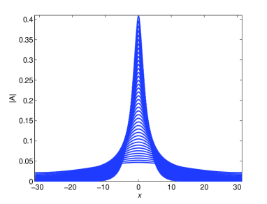
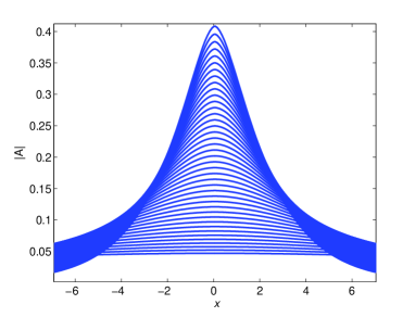
Refer to caption
Refer to caption
Figure 13: Left: Solution profiles for the nonlocal Ginzburg-Landau equation (6.6) with a Gaussian kernel for Σ=3Σ3\Sigma=3 along the lowest solution branch shown in figure 11. Right: enlargement of left-hand figure showing the evolution of the solutions near the point of blow-up. Other parameters are γ=1.0𝛾1.0\gamma=1.0, b2=2.0subscript𝑏22.0b_{2}=2.0. The domain size L=|Ω|=20π𝐿Ω20𝜋L=|\Omega|=20\pi.

In general, it is not a priori clear that (6.6) remains well-posed as the amplitude of solutions A(X)𝐴𝑋A(X) increases, due to the additional terms and the likelihood of singular behaviour for γΣ2|A|24𝛾superscriptΣ2superscript𝐴24\gamma\Sigma^{2}|A|^{2}\approx 4. This issue deserves detailed investigation, and we will return to it in future work. Its relevance to the formation of localised states is indicated by the (numerical) behaviour of solutions along the lowest (blue, solid) curve in figure 11. Solutions along this branch are shown in figure 13: solutions become increasingly sharp as their amplitude increases until numerical continuation fails to converge and the solution branch terminates. It is possible that this blow-up arises in a self-similar fashion.

The second natural distinguished limit that enables formation of a solvability condition at O(ε5)𝑂superscript𝜀5O\left(\varepsilon^{5}\right) is the choice β=2𝛽2\beta=2. In order to bring in the nonlocal terms at fifth order we combine this with a rescaling of the coefficient γ𝛾\gamma, writing γ=ε2γ2𝛾superscript𝜀2subscript𝛾2\gamma=\varepsilon^{2}\gamma_{2}. In this distinguished limit the resulting envelope equation, again choosing a Gaussian kernel, is

ATsubscript𝐴𝑇\displaystyle A_{T} =\displaystyle= μA+769b0b2A|A|28820361A|A|4+i1619AX|A|2𝜇𝐴769subscript𝑏0subscript𝑏2𝐴superscript𝐴28820361𝐴superscript𝐴4𝑖1619subscript𝐴𝑋superscript𝐴2\displaystyle\mu A+\frac{76}{9}b_{0}b_{2}A|A|^{2}-\frac{8820}{361}A|A|^{4}+i\frac{16}{19}A_{X}|A|^{2} (6.7)
2γ2An=1(2n1)!!(2n)!(ΣDX)2n|A|2+4AXX,2subscript𝛾2𝐴superscriptsubscript𝑛1double-factorial2𝑛12𝑛superscriptΣsubscript𝐷𝑋2𝑛superscript𝐴24subscript𝐴𝑋𝑋\displaystyle-2\gamma_{2}A\sum_{n=1}^{\infty}\frac{\left(2n-1\right)!!}{\left(2n\right)!}\left(\Sigma D_{X}\right)^{2n}|A|^{2}+4A_{XX},

where again b0=27/38subscript𝑏02738b_{0}=\sqrt{27/38}. The choice β=2𝛽2\beta=2 effectively makes the kernel act entirely on the long length scale X𝑋X and so every term in the series expansion (6.1) at the same order in ε𝜀\varepsilon. Formally, the series expansion is equivalent to the integral term, so that a more compact way of writing the amplitude equation is

ATsubscript𝐴𝑇\displaystyle A_{T} =\displaystyle= μA+769b0b2A|A|28820361A|A|4+i1619AX|A|2𝜇𝐴769subscript𝑏0subscript𝑏2𝐴superscript𝐴28820361𝐴superscript𝐴4𝑖1619subscript𝐴𝑋superscript𝐴2\displaystyle\mu A+\frac{76}{9}b_{0}b_{2}A|A|^{2}-\frac{8820}{361}A|A|^{4}+i\frac{16}{19}A_{X}|A|^{2} (6.8)
2γ2Ωe(XY)2/(2Σ2)|A(Y)|2𝑑Y+4AXX.2subscript𝛾2subscriptΩsuperscriptesuperscript𝑋𝑌22superscriptΣ2superscript𝐴𝑌2differential-d𝑌4subscript𝐴𝑋𝑋\displaystyle-2\gamma_{2}\int_{\Omega}\mathrm{e}^{-(X-Y)^{2}/(2\Sigma^{2})}|A(Y)|^{2}\ dY+4A_{XX}.

This nonlocal Ginzburg–Landau equation captures the nonlocal dynamics sufficiently strongly to reproduce aspects of the stretched and slanted snaking behaviour apparent in figures 3 and 4.
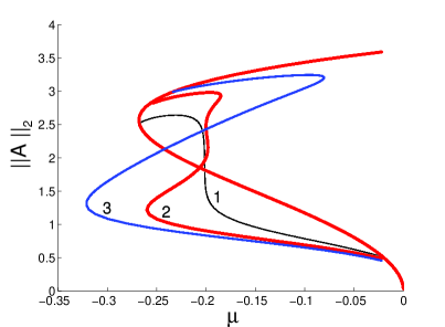
Refer to caption
Refer to caption
Figure 14: Left: Bifurcation diagram for solutions of the nonlocal Ginzburg-Landau equation (6.8) with a Gaussian kernel, for different values of the width parameter: Σ=0Σ0\Sigma=0 (black, labelled 1), Σ=3πΣ3𝜋\Sigma=3\pi (red, labelled 2) and Σ=10πΣ10𝜋\Sigma=10\pi (blue, labelled 3). Right: solution profiles for each curve of spatially modulated solutions at A2=2.5subscriptnorm𝐴22.5\|A\|_{2}=2.5, where the curves in (a) are close to intersecting. Note the central dip in the thick red curve (labelled 2). Other parameters are γ2=1.0subscript𝛾21.0\gamma_{2}=1.0, b2=1.0subscript𝑏21.0b_{2}=1.0. The domain size L=|Ω|=20π𝐿Ω20𝜋L=|\Omega|=20\pi.

Figure 14 contains bifurcation diagrams and solution profiles for three choices of ΣΣ\Sigma, moving from the purely local problem (Σ=0Σ0\Sigma=0, thin black curve) to nearly the global one (Σ=L/2Σ𝐿2\Sigma=L/2, medium thickness blue curve). For each value of ΣΣ\Sigma in figure 14(a), the curves of uniform constant solutions for |A|𝐴|A| are almost exactly superposed: of these only the thickest (red) curve is visible. The thin black line for the Σ=0Σ0\Sigma=0 case has a near-vertical central section, just as in figure 2. The thick red curve indicates how this vertical curve is deformed as the width of the nonlocal kernel is increased: the lower part moves to the left and the upper part to the right. This is exactly the behaviour observed for the homoclinic snaking in figures 4. The central section remains very close to the central section in the case Σ=0Σ0\Sigma=0. As the kernel width increases further we approach, smoothly, the slanted snaking limit in which the curve assumes its characteristic ‘Z’ shape. This transition takes place monotonically and smoothly, in contrast to the many disconnection and reconnection events associated with the homoclinic snaking curves themselves, and illustrated, for the top hat kernel, in figures 5 and 6. Figure 14(b) shows solution profiles |A(X)|𝐴𝑋|A(X)| on the three bifurcation curves in 14(a) at points close to where all three curves of spatially modulated solutions intersect. We see that the thickest (red) curve for intermediate kernel widths contains a central trough and off-centre peaks that are not present in the other two cases. This indicates the propensity of localised states for these intermediate kernel widths (more precisely, kernel widths that are longer than the basic wavelength of the pattern forming instability yet shorter than the width of the domain) to prefer to form multipulse states rather than single-pulse states. This therefore goes a little way towards justifying the collisions between the primary snaking curves and those of multipulse states described in figures 5 and 6.

7 Conclusions

In this paper we have considered equilibrium solutions, in the form of spatially localised states, to the one dimensional Swift–Hohenberg equation extended by a nonlocal term in convolution form. Numerical results suggested that the well known ‘homoclinic snaking’ structure was deformed and perturbed in several different ways as a result of the presence of nonlocality. We focussed our analytical efforts on extending the multiple-scales analysis for the Swift–Hohenberg equation to cope with the nonlocal term. Through (formal) expansions and application of Fourier transforms we were able to reduce the nonlocal integrodifferential Swift–Hohenberg equation into one of three Ginzburg–Landau-type equations that applied in different distinguished limits. These different limiting equations captured different aspects of the problem. As a direction for future work it would be of interest to link the results of Kao and Knobloch [18], which concern the behaviour of solutions to the cubic-quintic Ginzburg–Landau equation, to the parameter dependencies of the coefficients that the nonlocal terms produce.

While we focussed on two particular kernels, the ‘top hat’ composition of Heaviside step functions, and a Gaussian kernel, we present analytic results in as much generality as possible, writing the coefficients in the Ginzburg–Landau equations in terms of the Fourier transform of the kernel function. The Gaussian case can be motivated straightforwardly in applications since the convolution term is the solution of the initial value problem for the diffusion equation. The nonlocal term could then be thought of as directly modelling the diffusive spread of the solution, through interaction with another physical quantity, such as temperature, over timescales short compared to the time evolution of the Swift–Hohenberg equation itself.

On the mathematical side, it would be useful and interesting to extend results obtained recently by Achleitner and Kuehn [2] on the persistence of solutions in the presence of convolution terms, to prove that for kernels that are sufficiently narrow the homoclinic snaking bifurcation structure persists. Numerical work to investigate exactly the sequence of collisions with multipulse states for a specific choice of kernel would also be of interest.

Moreover, it would be desirable to extend the analysis of this one dimensional problem to two or three space dimensions, clearly of substantial physical relevance. There is plenty of room for optimism since Fourier transform results often extend easily to higher dimensions, so that such extensions may be achievable with largely similar techniques to those presented here. These and many other considerations in this complex problem are left to be the subject of future work.

Acknowledgements

JHPD gratefully acknowledges the support of the Royal Society through a University Research Fellowship.

References

  • [1] M. Abramowitz and I.A. Stegun, Handbook of Mathematical Functions with Formulas, Graphs, and Mathematical Tables. US. Nat. Bureau of Standards (1964)
  • [2] F. Achleitner and C. Kuehn. On bounded positive stationary solutions for a nonlocal Fisher–KPP equation. Preprint. arXiv: 1307.3480 (2013)
  • [3] D. Avitabile, D.J.B. Lloyd, J. Burke, E. Knobloch and B. Sandstede, To snake or not to snake in the planar Swift-Hohenberg equation. SIAM J. Appl. Dyn. Syst. 9, 704–733 (2010)
  • [4] J. Burke and E. Knobloch, Localized states in the generalized Swift–Hohenberg equation. Phys. Rev. E 73, 056211 (2006)
  • [5] J. Burke and J.H.P. Dawes, Localised states in an extended Swift–Hohenberg equation. SIAM J. Appl. Dyn. Syst. 11, 261–284 (2012)
  • [6] A. Champneys, Homoclinic orbits in reversible systems and their applications in mechanics, fluids and optics. Physica D 112, 158–186 (1998)
  • [7] S.J. Chapman and G. Kozyreff, Exponential asymptotics of localised patterns and snaking bifurcation diagrams. Physica D 238, 319–354 (2009)
  • [8] S. Coombes, G.J. Lord and M.R. Owen, Waves and bumps in neuronal networks with axo-dendritic synaptic interactions. Physica D 178, 219–241 (2003)
  • [9] P. Coullet, C. Riera and C. Tresser, Stable static localized structures in one dimension. Phys. Rev. Lett./ 84, 3069–3072 (2000)
  • [10] M. Cross and H. Greenside, Pattern Formation and Dynamics in Nonequilibrium Systems. CUP, Cambridge (2009)
  • [11] J.H.P. Dawes, The emergence of a coherent structure for coherent structures: localized states in nonlinear systems. Phil. Trans. R. Soc. Lond. A 368, 3519–3534 (2010)
  • [12] J.H.P. Dawes and H. Susanto, Variational approximation and the use of collective coordinates. Phys. Rev. E 87, 063202 (2013)
  • [13] A.D. Dean, P.C. Matthews, S.M. Cox and J.R. King, Exponential asymptotics of homoclinic snaking. Nonlinearity 24, 3323- 3351 (2011)
  • [14] E.J. Doedel, A.R. Champneys, T. Fairgrieve, Y. Kuznetsov, B. Oldeman, R. Paffenroth, B. Sandstede, X. Wang and C. Zhang, AUTO-07p: continuation and bifurcation software for ordinary differential equations. Available online at http://indy.cs.concordia.ca/auto/ (2011)
  • [15] W.J. Firth, L. Columbo and A.J. Scroggie, Proposed resolution of theory-experiment discrepancy in homoclinic snaking. Phys. Rev. Lett. 99, 104503 (2007)
  • [16] R.B. Hoyle, Pattern Formation: An introduction to methods. CUP, Cambridge (2006)
  • [17] A. Hutt and F.M. Atay, Analysis of nonlocal neural fields for both general and gamma-distributed connectivities. Physica D 203, 30–54 (2005)
  • [18] H.-C. Kao and E. Knobloch, Weakly subcritical stationary patterns: Eckhaus instability and homoclinic snaking. Phys. Rev. E 85, 026207 (2012)
  • [19] G. Kozyreff and S.J. Chapman, Asymptotics of large bound states of localized structures. Phys. Rev. Lett. 97, 044502 (2006)
  • [20] E.H. Lieb and M. Loss, Analysis. Graduate Studies in Mathematics Volume 14, Second Edition. AMS, Providence. (2010)
  • [21] P.C. Matthews and H. Susanto, Variational approximations to homoclinic snaking in continuous and discrete systems. Phys. Rev. E 84, 066207-11 (2011)
  • [22] E. Plaut and F.H. Busse, Low-Prandtl-number convection in a rotating cylindrical annulus. J. Fluid Mech. 464, 345–363 (2002)
  • [23] H.-G. Purwins, H.U. Bödeker and S. Amiranashvili, Dissipative solitons. Adv. Phys. 59, 485–701 (2010)
  • [24] H. Susanto and P.C. Matthews, Variational approximations to homoclinic snaking. Phys. Rev. E 83, 035201(R) (2011)
  • [25] C. Taylor and J.H.P. Dawes, Snaking and isolas of localised states in bistable discrete lattices. Phys. Lett. A 375, 14–22 (2010)
  • [26] U. Thiele, A.J. Archer, M.J. Robbins, H. Gomez and E. Knobloch, Localized states in the conserved Swift-Hohenberg equation with cubic nonlinearity, Phys. Rev. E 87, 042915 (2013)
  • [27] J. Vega, Instability of the steady states of some Ginzburg–Landau-like equations with real coefficients. Nonlinearity 18, 1425–1441 (2005)
  • [28] N.A. Venkov, S Coombes and P.C. Matthews, Dynamic instabilities in scalar neural field equations with space-dependent delays, Physica D 232, 1–15 (2007)
  • [29] P.D. Woods and A.R. Champneys, Heteroclinic tangles and homoclinic snaking in the unfolding of a degenerate reversible Hamiltonian–Hopf bifurcation. Physica D 129, 147–170 (1999)