Multi-leg One-loop Massive Amplitudes from Integrand Reduction via Laurent Expansion

Abstract:

We present the application of a novel reduction technique for one-loop scattering amplitudes based on the combination of the integrand reduction and Laurent expansion. We describe the general features of its implementation in the computer code Ninja, and its interface to GoSam. We apply the new reduction to a series of selected processes involving massive particles, from six to eight legs.

1 Introduction

Scattering amplitudes in quantum field theories are analytic functions of the kinematic variables of the interacting particles, hence they can be determined by studying the structure of their singularities.

The multi-particle factorization properties of the amplitudes become transparent when internal particles go on their mass-shell [1, 2]. These configurations correspond to poles of the amplitude and the investigation of the general structure of the residues corresponding to multi-particle factorization channel turns out to be of particular interest. Indeed the knowledge of such structure has been fundamental for discovering new relations fulfilled by scattering amplitudes, such as the BCFW recurrence relation [3] and its link to the leading singularity of one-loop amplitudes [4]. The systematic classification of the residues, for all the poles corresponding to the quadruple, triple, double, and single cuts, has been achieved, in four dimensions, by employing integrand-reduction methods [5, 6]. The latter led to the OPP integrand-decomposition formula for one-loop integrals [6], which allows one to write each residue as a linear combination of process-independent polynomials multiplied by process-dependent coefficients.

These results provided a deeper understanding of the structure of scattering amplitudes and have shown the underlying simplicity beneath the rich mathematical structure of quantum field theory. Moreover, they provided the theoretical framework for the development of efficient computational algorithms for one-loop calculations in perturbation theory, which have been implemented in various automated codes [7, 8, 9, 10, 11, 12, 13, 14, 15, 16] improving the state-of-the art of the predictions at the next-to-leading order accuracy [17, 18, 19, 20, 21, 22, 23, 24, 25, 26, 27, 28, 29, 30, 31, 32, 33, 34, 35, 36, 37, 38, 39, 40, 41, 42, 43, 44, 45, 46, 47, 48, 49, 50].

Recently, the classification of the structure of the residues has been obtained in a more general and elegant form within the framework of multivariate polynomial division and algebraic geometry [51, 52]. The use of these techniques proved that the integrand decomposition, originally formulated for one-loop amplitudes, is applicable at any order in perturbation theory, irrespective of the complexity of the topology of the diagrams involved. An iterative integrand-recursion formula, based on successive divisions of the numerators modulo the Gröbner basis of the ideals generated by the cut denominators, can provide the form of the residues at all multi-particle poles for arbitrary amplitudes, independently of the number of loops. Extensions of the integrand reduction method beyond one-loop, initiated in [53, 54] and then systematized within the language of algebraic geometry [51, 52] have recently become the topic of several studies [55, 56, 57, 58, 59, 60], thus providing a new direction in the study of multi-loop amplitudes.

In the context of the integrand reduction, the process-dependent coefficients can be numerically determined by solving a system of algebraic equations that are obtained by evaluating the numerator of the integrand at explicit values of the loop momentum [6]. The system becomes triangular if one evaluates the numerator at the multiple cuts, i.e. at the set of complex values of the integration momentum for which a given set of propagators vanish. The extraction of all coefficients via polynomial fitting has been implemented in publicly available codes performing integrand decomposition, such as CutTools [61] and Samurai [62]. These algorithms do not require any specific recipe for the generation of the numerator function, which can be performed by using traditional Feynman diagrams, by means of recursive relations, or by gluing tree-level sub-amplitudes, as in unitarity-based methods.

The code CutTools implements the four-dimensional integrand-reduction algorithm [63, 64, 65], in which the cut-constructible term and the rational term are necessarily computed separately. The latter escapes four-dimensional integrand reduction and has to be computed by means of other methods, e.g. ad hoc tree-level Feynman rules [65, 66, 67, 68, 69, 70, 71, 72].

Significant improvements were achieved with the $d$-dimensional extension of integrand-reduction methods [73, 74, 75], which expose a richer polynomial structure of the integrand and allows for the combined determination of both cut-constructible and rational terms at once. This idea of performing unitarity-cuts in $d$-dimension was the basis for the development of Samurai, which extends the OPP polynomial structures to include an explicit dependence on the $(d-4)$-dimensional parameter needed for the automated computation of the full rational term. Moreover, it includes the parametrization of the residue of the quintuple-cut [76] and implements the numerical sampling via Discrete Fourier Transform [64].

The integrand decomposition was originally developed for renormalizable gauge theories, where, at one-loop, the rank of the numerator cannot be larger than the number of external legs. The reduction of diagrams where the rank can be higher, as required for example when computing $pp\to H+2,3$ jets in gluon fusion in the large top-mass limit [42, 44], demands an extension of the algorithm to accommodate the richer monomial structures of the residues. This extension has been implemented in Samurai, together with the corresponding sampling required to fit all the coefficients [77, 78, 79].

More recently, elaborating on the the techniques proposed in [80, 81], a different approach to the $d$-dimensional integrand-reduction method was proposed [78]. The key point of this method is to extract the coefficients more efficiently by performing a Laurent expansion of the integrand. The method is general and relies only on the knowledge of the explicit dependence of the numerator on the loop momentum.

In general, when the multiple-cut conditions do not fully constrain the loop momentum, the solutions are still functions of some free parameters, possibly the components of the momentum which are not frozen by the cut conditions. The integrand-reduction algorithms implemented in the codes [61, 62] require to solve a system of equations obtained by sampling on those free parameters. The system is triangular thus the coefficients of a given residue can be computed only after subtracting all the non-vanishing contributions coming from higher-point residues.

The key observation suggested in Ref.[78] is that the reduction algorithm can be simplified by exploiting the universal structure of the residues, hence of their asymptotic expansion. Indeed, by performing a Laurent expansion with respect to one of the free parameters which appear in the solutions of the cut, both the integrand and the subtraction terms exhibit the same polynomial behavior of the residue. Moreover, the contributions coming from the subtracted terms can be implemented as corrections at the coefficient level, hence replacing the subtractions at the integrand level of the original algorithm. The parametric form of these corrections can be computed once and for all, in terms of a subset of the higher-point coefficients. This method significantly reduces the number of coefficients entering each subtracted term, in particular boxes and pentagons decouple from the computation of lower-points coefficients.

If either the analytic expression of the integrand or the tensor structure of the numerator is known, this procedure can be implemented in a semi-numerical algorithm. Indeed, the coefficients of the Laurent expansion of a rational function can be computed, either analytically or numerically, by performing a polynomial division between the numerator and the (uncut) denominators.

The scope of the present paper is to review the main features of the novel reduction algorithm and demonstrate its performance on a selection of challenging calculations of scattering amplitudes with massive bosons and quarks, involving six, seven, and eight particles. The integrand-reduction via Laurent expansion has been implemented in the c++ library Ninja [82, 83], and interfaced to the GoSam framework [12] for the evaluation of virtual one-loop scattering amplitudes. The cleaner and lighter system-solving strategy, which deals with a diagonal system instead of a triangular one, and which substitutes the polynomial subtractions with coefficients corrections, turns into net gains in terms of both numerical accuracy and computing speed. We recall that the new library has been recently used in the evaluation of NLO QCD corrections to $pp\to t{\bar{t}}Hj$ [45].

The paper is organized as follows. In Section 2, we discuss the theoretical foundations of the integrand decomposition via Laurent expansion, and its implementation in an algorithm for the reduction of one-loop amplitudes. The description of the interface between Ninja and GoSam for automated one-loop calculation is discussed in Section 3. Section 4 is devoted to a detailed study of the precision and of the computational performance of the novel framework, which shows a significant improvement with respect to the standard algorithms. Applications of the GoSam+Ninja framework to the evaluation of NLO QCD virtual correction to several multi-leg massive processes are shown in Section 5.

2 Reduction Algorithm – Integrand Reduction via Laurent Expansion

In this section we describe the Laurent-expansion method for the integrand reduction of one-loop amplitudes as implemented in the C++ library Ninja.

2.1 Integrand and Integral decomposition

An $n$-point one-loop amplitude can be written as a linear combination of contributions $\mathcal{M}_{1\cdots n}$ of the form

$$\mathcal{M}_{1\cdots n}=\int d^{d}\bar{q}\;\mathcal{I}_{1\cdots n}=\int d^{d}\bar{q}\,\frac{\mathcal{N}(\bar{q})}{D_{1}\cdots D_{n}}$$ (1)

where $\mathcal{N}(\bar{q})$ is a process-dependent polynomial numerator in the components of the $d=(4-2\epsilon)$-dimensional loop momentum $\bar{q}$. The latter can be decomposed as follows,

$$\bar{\not{q}}={\not{q}}+{\not{\mu}}\ ,\qquad\bar{q}^{2}=q^{2}-\mu^{2}\ ,$$ (2)

in terms of its $4$-dimensional component, $q$, and $\mu^{2}$ which encodes its $(-2\epsilon)$-dimensional components. The denominators $D_{i}$ are quadratic polynomials in $\bar{q}$ and correspond to Feynman loop propagators,

$$D_{i}=(\bar{q}+p_{i})^{2}-m_{i}^{2}.$$ (3)

Every one-loop integrand in $d$ dimensions can be decomposed as [6, 73]

$$\mathcal{I}_{1\ldots n}\equiv\frac{\mathcal{N}_{1\cdots n}}{D_{1}\ldots D_{n}}=\sum_{k=1}^{5}\sum_{\{i_{1},\cdots,i_{k}\}}\frac{\Delta_{i_{1}\cdots i_{k}}}{D_{i_{1}}\cdots D_{i_{k}}},$$ (4)

where the $\Delta_{i_{1}\cdots i_{k}}$ are irreducible polynomial residues, i.e. polynomials which do not contain any term proportional to the corresponding loop denominators $D_{i_{1}},\ldots,D_{i_{k}}$. The second sum in Eq. (4) runs over all unordered selections without repetition of the $k$ indices $\{i_{1},\cdots,i_{k}\}$.

For any set of denominators $D_{i_{1}},\ldots,D_{i_{k}}$ with $k\leq 5$, one can choose a $4$-dimensional basis of momenta $\mathcal{E}=\{e_{1},e_{2},e_{3},e_{4}\}$ which satisfies the following normalization conditions

$$e_{1}\cdot e_{2}=1,\qquad e_{3}^{2}=e_{4}^{2}=\delta_{k4},\qquad e_{3}\cdot e_{4}=-(1-\delta_{k4}),$$ (5)

while all the other scalar products vanish. In addition, for $k=4$ we choose the basis such that $e_{4}$ is orthogonal to the external legs of the sub-diagram identified by the set of denominators in consideration. Similarly, for $k=2,3$ we choose both $e_{3}$ and $e_{4}$ to be orthogonal to the external legs of the corresponding sub-diagram. With this choices of momentum basis, the numerator and the denominators can be written as polynomials in the coordinates $\mathbf{z}\equiv(z_{1},z_{2},z_{3},z_{4},z_{5})=(x_{1},x_{2},x_{3},x_{4},\mu^{2})$. The variables $x_{i}$ are the components of $q$ with respect to the basis $\mathcal{E}$,

$$q^{\nu}=-p^{\nu}_{i_{1}}+x_{1}\ e^{\nu}_{1}+x_{2}\ e^{\nu}_{2}+x_{3}\ e^{\nu}_{3}+x_{4}\ e^{\nu}_{4}\ .$$ (6)

More explicitly, the numerator is a polynomial in the components of $q$ and $\mu^{2}$

$$\mathcal{N}(\bar{q})=\mathcal{N}(q,\mu^{2})=\mathcal{N}(x_{1},x_{2},x_{3},x_{4},\mu^{2})=\mathcal{N}(\mathbf{z}).$$ (7)

The coordinates $x_{i}$ can also be written as scalar products,

$$x_{1} =(q+p_{i_{1}})\cdot e_{2}$$

$$x_{2} =(q+p_{i_{1}})\cdot e_{1}$$

$$x_{3} =-((q+p_{i_{1}})\cdot e_{4})(1-\delta_{k4})+((q+p_{i_{1}})\cdot e_{3})\delta_{k4}$$

$$x_{4} =-((q+p_{i_{1}})\cdot e_{3})(1-\delta_{k4})+((q+p_{i_{1}})\cdot e_{4})\delta_{k4}.$$ (8)

With these definitions, one can show [6, 73, 51] that the most general parametric form of a residue in a renormalizable theory is

$$\Delta_{i_{1}i_{2}i_{3}i_{4}i_{5}}={} c^{(i_{1}i_{2}i_{3}i_{4}i_{5})}_{0}\,\mu^{2}$$

$$\Delta_{i_{1}i_{2}i_{3}i_{4}}={} c^{(i_{1}i_{2}i_{3}i_{4})}_{0}+c^{(i_{1}i_{2}i_{3}i_{4})}_{1}x_{4}+\mu^{2}\left(c^{(i_{1}i_{2}i_{3}i_{4})}_{2}+c^{(i_{1}i_{2}i_{3}i_{4})}_{3}x_{4}+\mu^{2}c^{(i_{1}i_{2}i_{3}i_{4})}_{4}\right)$$

$${\Delta}_{i_{1}i_{2}i_{3}}={} c^{(i_{1}i_{2}i_{3})}_{0}+c^{(i_{1}i_{2}i_{3})}_{1}x_{3}+c^{(i_{1}i_{2}i_{3})}_{2}x_{3}^{2}+c^{(i_{1}i_{2}i_{3})}_{3}x_{3}^{3}+c^{(i_{1}i_{2}i_{3})}_{4}x_{4}+c^{(i_{1}i_{2}i_{3})}_{5}x_{4}^{2}$$

$$+c^{(i_{1}i_{2}i_{3})}_{6}x_{4}^{3}+\mu^{2}\left(c^{(i_{1}i_{2}i_{3})}_{7}+c^{(i_{1}i_{2}i_{3})}_{8}x_{3}+c^{(i_{1}i_{2}i_{3})}_{9}x_{4}\right)$$

$${\Delta}_{i_{1}i_{2}}={} c^{(i_{1}i_{2})}_{0}+c^{(i_{1}i_{2})}_{1}x_{2}+c^{(i_{1}i_{2})}_{2}x_{3}+c^{(i_{1}i_{2})}_{3}x_{4}+c^{(i_{1}i_{2})}_{4}x^{2}_{2}+c^{(i_{1}i_{2})}_{5}x^{2}_{3}$$

$$+c^{(i_{1}i_{2})}_{6}x^{2}_{4}+c^{(i_{1}i_{2})}_{7}x_{2}x_{3}+c^{(i_{1}i_{2})}_{8}x_{2}x_{4}+c^{(i_{1}i_{2})}_{9}\mu^{2}$$

$${\Delta}_{i_{1}}={} c^{(i_{1})}_{0}+c^{(i_{1})}_{1}x_{1}+c^{(i_{1})}_{2}x_{2}+c^{(i_{1})}_{3}x_{3}+c^{(i_{1})}_{4}x_{4}.$$ (9)

This parametric form can also be extended to non-renormalizable and effective theories, where the rank of the numerator can be larger than the number of loop propagators [78]. Most of the term appearing in Eq. (9) vanish after integration, i.e. they are spurious. The non-spurious coefficients, instead, appear in the final result which expresses the amplitude $\mathcal{M}_{1\cdots n}$ as a linear combination of known Master Integrals,

$$\mathcal{M}_{1\cdots n}={} \sum_{\{i_{1},i_{2},i_{3},i_{4}\}}\bigg{\{}c_{0}^{(i_{1}i_{2}i_{3}i_{4})}I_{i_{1}i_{2}i_{3}i_{4}}+c_{4}^{(i_{1}i_{2}i_{3}i_{4})}I_{i_{1}i_{2}i_{3}i_{4}}[\mu^{4}]\bigg{\}}$$

$$+\sum_{\{i_{1},i_{2},i_{3}\}}^{n-1}\bigg{\{}c_{0}^{(i_{1}i_{2}i_{3})}I_{i_{1}i_{2}i_{3}}+c_{7}^{(i_{1}i_{2}i_{3})}I_{i_{1}i_{2}i_{3}}[\mu^{2}]\bigg{\}}$$

$$+\sum_{\{i_{1},i_{2}\}}\bigg{\{}c_{0}^{(i_{1}i_{2})}I_{i_{1}i_{2}}+c_{1}^{(i_{1}i_{2})}I_{i_{1}i_{2}}[(q+p_{i_{1}})\cdot e_{2}]$$

$$\qquad+c_{2}^{(i_{1}i_{2})}I_{i_{1}i_{2}}[((q+p_{i_{1}})\cdot e_{2})^{2}]+c_{9}^{(i_{1}i_{2})}I_{i_{1}i_{2}}[\mu^{2}]\bigg{\}}$$

$$+\sum_{i_{1}}c_{0}^{(i_{1})}I_{i_{1}},$$ (10)

where

$$I_{i_{1}\cdots i_{k}}[\alpha]\equiv\int d^{d}\bar{q}{\alpha\over D_{i_{1}}\cdots D_{i_{k}}},\qquad I_{i_{1}\cdots i_{k}}\equiv I_{i_{1}\cdots i_{k}}[1].$$

The problem of the computation of any one-loop amplitude can therefore be reduced to the problem of the determination of the coefficients of the Master Integrals appearing in Eq. (10), which in turn can be identified with a subset of the coefficients of the parametric residues in Eq. (9).

2.2 Scattering amplitudes via Laurent expansion

In Ref. [78], elaborating on the the techniques proposed in [80, 81], an improved version of the integrand-reduction method for one-loop amplitudes was presented. This method allows, whenever the analytic dependence of the integrand on the loop momentum is known, to extract the unknown coefficients of the residues $\Delta_{i_{1}\cdots i_{k}}$ by performing a Laurent expansion of the integrand with respect to one of the free loop components which are not constrained by the corresponding on-shell conditions $D_{i_{1}}=\cdots=D_{i_{k}}=0$.

Within the original integrand reduction algorithm [61, 64, 62], the determination of these unknown coefficients requires: i) to sample the numerator on a finite subset of the on-shell solutions; ii) to subtract from the integrand the non-vanishing contributions coming from higher-point residues; and iii) to solve the resulting linear system of equations.

With the Laurent-expansion approach, since in the asymptotic limit both the integrand and the higher-point subtractions exhibit the same polynomial behavior as the residue, one can instead identify the unknown coefficients with the ones of the expansion of the integrand, corrected by the contributions coming from higher-point residues. In other words, the system of equations for the coefficients becomes diagonal and the subtractions of higher-point contributions can be implemented as corrections at the coefficient level which replace the subtractions at the integrand level of the original algorithm. Because of the universal structure of the residues, the parametric form of these corrections can be computed once and for all, in terms of a subset of the higher-point coefficients. This also allows to significantly reduce the number of coefficients entering in each subtraction. For instance, box and pentagons do not affect at all the computation of lower-points residues. In the followings, we describe in more detail how to determine the needed coefficients of each residue.

Pentagons

Pentagons contributions are spurious, i.e. they do not appear in the integrated result. In the original integrand reduction algorithm their computation is nevertheless needed, in order to implement the corresponding subtractions at the integrand level. Within the Laurent expansion approach, since the subtraction terms of five-point residues always vanish in the asymptotic limit, their computation is instead not needed and can be skipped.

Boxes

The coefficient $c_{0}$ of the box contributions can be determined via 4-dimensional quadruple cuts [4]. In four dimensions (i.e. $\bar{q}=q$, $\mu^{2}=0$) a quadruple cut $D_{i_{1}}=\cdots=D_{i_{4}}=0$ has two solutions, $q_{+}$ and $q_{-}$. The coefficient $c_{0}$ can be expressed in terms of these solutions as

$$c^{(i_{1}i_{2}i_{3}i_{4})}_{0}=\frac{1}{2}\left(\left.\frac{\mathcal{N}(q)}{\prod_{j\neq i_{1},i_{2},i_{3},i_{4}}D_{j}}\right|_{q=q_{+}}+\left.\frac{\mathcal{N}(q)}{\prod_{j\neq i_{1},i_{2},i_{3},i_{4}}D_{j}}\right|_{q=q_{-}}\right).$$ (11)

The coefficient $c_{4}$ can be found by evaluating the integrand on $d$-dimensional quadruple cuts in the asymptotic limit $\mu^{2}\rightarrow\infty$ [81]. A $d$-dimensional quadruple cut has an infinite number of solutions which can be parametrized by the extra-dimensional variable $\mu^{2}$. These solutions become particularly simple in the limit of large $\mu^{2}$, namely

$$q_{\pm}^{\nu}=a^{\nu}\pm\sqrt{\mu^{2}+\beta}\,e_{4}^{\nu}\;\overset{\mu^{2}\rightarrow\infty}{\longrightarrow}\;\pm\sqrt{\mu^{2}}\,e_{4}^{\nu}+\mathcal{O}(1)$$ (12)

where the vector $a^{\nu}$ and the constant $\beta$ are fixed by the cut conditions. The coefficient $c_{4}$, when non-vanishing, can be found in this limit as the leading term of the expansion of the integrand

$$\frac{\mathcal{N}(q,\mu^{2})}{\prod_{j\neq i_{1},i_{2},i_{3},i_{4}}D_{j}}\;\overset{\mu^{2}\rightarrow\infty}{\longrightarrow}\;c^{(i_{1}i_{2}i_{3}i_{4})}_{4}\,\mu^{4}+\mathcal{O}(\mu^{3}).$$ (13)

The other coefficients of the boxes are spurious and their computation can be avoided.

Triangles

The residues of the triangle contributions can be determined by evaluating the integrand on the solutions of $d$-dimensional triple cuts [80], which can be parametrized by the extra-dimensional variable $\mu^{2}$ and another parameter $t$,

$$q_{+}=a^{\nu}+t\,e_{3}^{\nu}+\frac{\beta+\mu^{2}}{2\,t}\,e_{4}^{\nu},\qquad q_{-}=a^{\nu}+\frac{\beta+\mu^{2}}{2\,t}\,e_{3}^{\nu}+t\,e_{4}^{\nu},$$ (14)

where the vector $a^{\nu}$ and the constant $\beta$ are fixed by the cut conditions $D_{i_{1}}=D_{i_{2}}=D_{i_{3}}=0$. On these solutions, the integrand generally receives contributions from the residue of the triple cut $\Delta_{i_{1}i_{2}i_{3}}$, as well as from the boxes and pentagons which share the three cut denominators. However, after taking the asymptotic expansion at large $t$ and dropping the terms which vanish in this limit, the pentagon contributions vanish, while the box contributions are constant in $t$ but vanish when taking the average between the parametrizations $q_{+}$ and $q_{-}$ of Eq. (14). More explicitly,

$$\frac{\mathcal{N}(q_{\pm},\mu^{2})}{\prod_{j\neq i_{1},i_{2},i_{3}}D_{j}} =\Delta_{i_{1}i_{2}i_{3}}+{} {}\sum_{j}\frac{\Delta_{i_{1}i_{2}i_{3}j}}{D_{j}} +\sum_{jk}\frac{\Delta_{i_{1}i_{2}i_{3}jk}}{D_{j}D_{k}}$$

$$=\Delta_{i_{1}i_{2}i_{3}}+{} {}d_{1}^{\pm}+d_{2}^{\pm}\,\mu^{2} +\mathcal{O}(1/t),\quad\qquad\textrm{with }d_{i}^{+}+d_{i}^{-}=0.$$ (15)

Moreover, even though the integrand is a rational function, in this asymptotic limit it exhibits the same polynomial behavior as the expansion of the residue $\Delta_{i_{1}i_{2}i_{3}}$,

$$\frac{\mathcal{N}(q_{+},\mu^{2})}{\prod_{j\neq i_{1},i_{2},i_{3}}D_{j}}={} n_{0}^{+}+n_{7}^{+}\,\mu^{2}-(n_{4}+n_{9}\,\mu^{2})\,{t}+n_{5}\,{t^{2}}+n_{6}\,{t^{3}}+\mathcal{O}(1/{t})$$

$$\frac{\mathcal{N}(q_{-},\mu^{2})}{\prod_{j\neq i_{1},i_{2},i_{3}}D_{j}}={} n_{0}^{-}+n_{7}^{-}\,\mu^{2}-(n_{1}+n_{8}\,\mu^{2})\,{t}+n_{2}\,{t^{2}}+n_{3}\,{t^{3}}+\mathcal{O}(1/{t})$$ (16)

$$\Delta_{i_{1}i_{2}i_{3}}(q_{+},\mu^{2})={} c^{(i_{1}i_{2}i_{3})}_{0}+c^{(i_{1}i_{2}i_{3})}_{7}\,\mu^{2}-(c^{(i_{1}i_{2}i_{3})}_{4}+c^{(i_{1}i_{2}i_{3})}_{9}\,\mu^{2})\,{t}$$

$$+c^{(i_{1}i_{2}i_{3})}_{5}\,{t^{2}}-c^{(i_{1}i_{2}i_{3})}_{6}\,{t^{3}}+\mathcal{O}(1/{t})$$

$$\Delta_{i_{1}i_{2}i_{3}}(q_{-},\mu^{2})={} c^{(i_{1}i_{2}i_{3})}_{0}+c^{(i_{1}i_{2}i_{3})}_{7}\,\mu^{2}-(c^{(i_{1}i_{2}i_{3})}_{1}+c^{(i_{1}i_{2}i_{3})}_{8}\,\mu^{2})\,{t}$$

$$+c^{(i_{1}i_{2}i_{3})}_{2}\,{t^{2}}-c^{(i_{1}i_{2}i_{3})}_{3}\,{t^{3}}+\mathcal{O}(1/{t}).$$ (17)

By comparison of Eq.s (16), (17) and (15) one gets all the triangle coefficients as

$$c^{(i_{1}i_{2}i_{3})}_{i}=\frac{1}{2}(n_{i}^{+}+n_{i}^{-})\quad\textrm{for $i=0,7$,}\qquad c^{(i_{1}i_{2}i_{3})}_{i}=n_{i}\quad\textrm{for $i\neq 0,7$}.$$ (18)

It is worth to observe that, within the Laurent expansion approach, the determination of the 3-point residues does not require any subtraction of higher-point terms.

Bubbles

The on-shell solutions of a $d$-dimensional double cut $D_{i_{1}}=D_{i_{2}}=0$ can be parametrized as

$$q_{+} =a_{0}^{\nu}+x\,a_{1}^{\nu}+t\,e_{3}^{\nu}+\frac{\beta_{0}+\beta_{1}\,x+\beta_{2}\,x^{2}+\mu^{2}}{2\,t}\,e_{4}^{\nu},$$

$$q_{-} =a_{0}^{\nu}+x\,a_{1}^{\nu}+\frac{\beta_{0}+\beta_{1}\,x+\beta_{2}\,x^{2}+\mu^{2}}{2\,t}\,e_{3}^{\nu}+t\,e_{4}^{\nu},$$ (19)

in terms of the three free parameters $x$, $t$ and $\mu^{2}$, while the vectors $a_{i}^{\nu}$ and the constants $\beta_{i}$ are fixed by the on-shell conditions. After evaluating the integrand on these solutions and taking the asymptotic limit $t\rightarrow\infty$, the only non-vanishing subtraction terms come from the triangle contributions,

$$\frac{\mathcal{N}(q_{\pm},\mu^{2})}{\prod_{j\neq i_{1},i_{2}}D_{j}} =\Delta_{i_{1}i_{2}}+\sum_{j}\frac{\Delta_{i_{1}i_{2}j}}{D_{j}}+\sum_{jk}\frac{\Delta_{i_{1}i_{2}jk}}{D_{j}D_{k}}+\sum_{jkl}\frac{\Delta_{i_{1}i_{2}jkl}}{D_{j}D_{k}D_{l}}$$

$$=\Delta_{i_{1}i_{2}}+\sum_{j}\frac{\Delta_{i_{1}i_{2}j}}{D_{j}}+\mathcal{O}(1/t).$$ (20)

The integrand and the subtraction term are rational function, but in the asymptotic limit they both have the same polynomial behavior as the residue, namely

$$\frac{\mathcal{N}(q_{+},\mu^{2})}{\prod_{j\neq i_{1},i_{2}}D_{j}}={} n_{0}+n_{9}\,{\mu^{2}}+n_{1}\,{x}+n_{2}\,{x^{2}}-\big{(}n_{5}+n_{8}{x}\big{)}{t}+n_{6}\,{t^{2}}+\mathcal{O}(1/{t})$$

$$\frac{\mathcal{N}(q_{-},\mu^{2})}{\prod_{j\neq i_{1},i_{2}}D_{j}}={} n_{0}+n_{9}\,{\mu^{2}}+n_{1}\,{x}+n_{2}\,{x^{2}}-\big{(}n_{3}+n_{7}{x}\big{)}{t}+n_{4}\,{t^{2}}+\mathcal{O}(1/{t})$$ (21)

$$\frac{\Delta_{i_{1}i_{2}j}(q_{+},\mu^{2})}{D_{j}}={} c_{s,0}^{(j)}+c_{s,9}^{(j)}\,{\mu^{2}}+c_{s,1}^{(j)}\,{x}+c_{s,2}^{(j)}\,{x^{2}}-\big{(}c_{s,5}^{(j)}+c_{s,8}^{(j)}{x}\big{)}{t}+c_{s,6}^{(j)}\,{t^{2}}+\mathcal{O}(1/{t})$$

$$\frac{\Delta_{i_{1}i_{2}j}(q_{-},\mu^{2})}{D_{j}}={} c_{s,0}^{(j)}+c_{s,9}^{(j)}\,{\mu^{2}}+c_{s,1}^{(j)}\,{x}+c_{s,2}^{(j)}\,{x^{2}}-\big{(}c_{s,3}^{(j)}+c_{s,7}^{(j)}{x}\big{)}{t}+c_{s,4}^{(j)}\,{t^{2}}+\mathcal{O}(1/{t})$$ (22)

$$\Delta_{i_{1}i_{2}}(q_{+},\mu^{2})={} c^{(i_{1}i_{2})}_{0}+c^{(i_{1}i_{2})}_{9}\,{\mu^{2}}+c^{(i_{1}i_{2})}_{1}\,{x}+c^{(i_{1}i_{2})}_{2}{x^{2}}-\big{(}c^{(i_{1}i_{2})}_{5}+c^{(i_{1}i_{2})}_{8}{x}\big{)}\,{t}$$

$$+c^{(i_{1}i_{2})}_{6}\,{t^{2}}+\mathcal{O}(1/{t})$$

$$\Delta_{i_{1}i_{2}}(q_{-},\mu^{2})={} c^{(i_{1}i_{2})}_{0}+c^{(i_{1}i_{2})}_{9}\,{\mu^{2}}+c^{(i_{1}i_{2})}_{1}\,{x}+c^{(i_{1}i_{2})}_{2}{x^{2}}-\big{(}c^{(i_{1}i_{2})}_{3}+c^{(i_{1}i_{2})}_{7}{x}\big{)}\,{t}$$

$$+c^{(i_{1}i_{2})}_{4}\,{t^{2}}+\mathcal{O}(1/{t}).$$ (23)

The coefficients $c_{s,i}^{(j)}$ of the Laurent expansion of the subtractions terms in Eq.s (22) can be computed once and for all as parametric functions of the triangles coefficients. Therefore, the subtraction of the triangles can be implemented as corrections to the coefficients of the expansion of the integrand. Indeed, by inserting Eq.s (21), (22) and (23) in Eq. (20) one gets

$$c^{(i_{1}i_{2})}_{i}=n_{i}-\sum_{j}c_{s,i}^{(j)}\quad\textrm{for $i=0,\ldots,9$}.$$ (24)

Tadpoles

Once the coefficients of the triangles and the bubbles are known, one can determine the non-spurious coefficient $c_{0}$ of a tadpole residue $\Delta_{i_{1}}$ by evaluating the integrand on the single cut $D_{i_{1}}=0$. One can choose 4-dimensional solutions of the form

$$q^{\nu}_{+}=-p_{i_{1}}^{\nu}+t\,e_{3}^{\nu}+\frac{\beta}{2\,t}\,e_{4}^{\nu}$$ (25)

parametrized by the free variable $t$, while the constant $\beta$ is fixed by the cut conditions. In the asymptotic limit $t\rightarrow\infty$, only bubbles and triangles coefficients are non-vanishing,

$$\frac{\mathcal{N}(q_{+})}{\prod_{j\neq i_{1}}D_{j}} =\Delta_{i_{1}}+\sum_{j}\frac{\Delta_{i_{1}j}}{D_{j}}+\sum_{jk}\frac{\Delta_{i_{1}jk}}{D_{j}D_{k}}+\sum_{jkl}\frac{\Delta_{i_{1}jkl}}{D_{j}D_{k}D_{l}}$$

$$=\Delta_{i_{1}}+\sum_{j}\frac{\Delta_{i_{1}j}}{D_{j}}+\sum_{jk}\frac{\Delta_{i_{1}jk}}{D_{j}D_{k}}+\mathcal{O}(1/t).$$ (26)

Similarly to the case of the bubbles, in this limit the integrand and the subtraction terms exhibit the same polynomial behavior as the residue, i.e.

$$\frac{\mathcal{N}(q_{+})}{\prod_{j\neq i_{1}}D_{j}} =n_{0}-n_{4}\,t+\mathcal{O}(1/t)$$ (27)

$$\frac{\Delta_{i_{1}j}(q_{+})}{D_{j}} =c_{s_{2},0}^{(j)}-c_{s_{2},4}^{(j)}\,t+\mathcal{O}(1/t)$$ (28)

$$\frac{\Delta_{i_{1}jk}(q_{+})}{D_{j}D_{k}} =c_{s_{3},0}^{(jk)}-c_{s_{3},4}^{(jk)}\,t+\mathcal{O}(1/t)$$ (29)

$$\Delta_{i_{1}}(q_{+}) =c^{(i_{1})}_{0}-c^{(i_{1})}_{4}\,t.$$ (30)

Putting everything together, we can write the coefficient of the tadpole integral as the corresponding one in the expansion of the integrand, corrected by coefficient-level subtractions

$$c^{(i_{1})}_{0}=n_{0}-\sum_{j}c_{s_{2},0}^{(j)}-\sum_{jk}c_{s_{3},0}^{(jk)}.$$ (31)

Once again, we observe that the subtraction terms $c_{s_{2},0}^{(j)}$ and $c_{s_{3},0}^{(jk)}$, coming from bubbles and triangles contributions respectively, are known parametric functions of the coefficients of the corresponding higher-point residues.

2.3 The C++ library Ninja

The C++ library Ninja [82, 83] provides a semi-numerical implementation of the Laurent expansion method described above. Since the integrand is a rational function of the loop variables, its Laurent expansion is performed via a simplified polynomial division algorithm between the expansion of the numerator $\mathcal{N}$ and the uncut denominators.

The inputs of the reduction algorithm implemented in Ninja are the external momenta $p_{i}$ and the masses $m_{i}$ of the loop denominators defined in Eq. (3), and the numerator $\mathcal{N}(q,\mu^{2})$ of the integrand cast in four different forms.

• The first form provides a simple evaluation of the numerator as a function of $q$ and $\mu^{2}$, which is used in order to compute the coefficient $c_{0}$ of the boxes. It can also be used in order to compute the spurious coefficients of the pentagons via penta-cuts, and all the ones of the boxes when the expansion in $\mu^{2}$ is not provided.

The other three forms of the numerator yield instead the leading terms of a parametric expansion of the integrand.

• The first expansion is the one used in order to obtain the coefficient $c_{4}$ of the boxes. When the rank $r$ is equal to the number $n$ of external legs of the diagram, this method returns the coefficient of $t^{n}$ obtained by substituting in the numerator $\mathcal{N}(q,\mu^{2})$

  $$q^{\nu}\rightarrow t\,v^{\nu},\qquad\mu^{2}\rightarrow t^{2}\,v^{2}$$ (32)

  as a function of a generic vector $v$, which is computed by Ninja and is determined by the quadruple-cut constraints.

• The second expansion is used in order to compute triangles and tadpole coefficients. In this case it returns coefficients of the terms $t^{j}\mu^{2k}$ for $j=r,r-1,\ldots,n-3$, obtained from $\mathcal{N}(q,\mu^{2})$ with the substitutions

  $$q^{\nu}\rightarrow v_{0}^{\nu}+t\,v_{3}^{\nu}+\frac{\beta+\mu^{2}}{t}\,v_{4}^{\nu},\qquad v_{3}^{2}=v_{4}^{2}=0,$$ (33)

  as a function of the generic momenta $v_{i}^{\nu}$ and the constant $\beta_{0}$. Since in a renormalizable theory $r\leq n$, and by definition of rank we have $j+2k\leq r$, at most 6 terms can be non-vanishing in the specified range of $j$. For effective theories with $r\leq n+1$, one can have instead up to 9 non-vanishing polynomial terms. In each call of the numerator, Ninja specifies the lowest power of $t$ which is needed in the evaluation, avoiding thus the computation of unnecessary coefficients of the expansion.

• The third and last expansion is needed for the computation of the 2-point residues and returns the coefficients of the terms $t^{j}\mu^{2k}x^{l}$ for $j=r,r-1,\ldots,n-2$, obtained from $\mathcal{N}(q,\mu^{2})$ with the substitutions

  $$q^{\nu}\rightarrow v_{1}^{\nu}+x\,v_{2}^{\nu}+t\,v_{3}^{\nu}+\frac{\beta_{0}+\beta_{1}\,x+\beta_{2}\,x^{2}+\mu^{2}}{t}\,v_{4}^{\nu},\qquad v_{2}\cdot v_{3}=v_{2}\cdot v_{4}=v_{3}^{2}=v_{4}^{2}=0,$$ (34)

  as a function of the cut-dependent momenta $v_{i}^{\nu}$ and constants $\beta_{i}$. In a renormalizable theory one can have at most 7 non-vanishing terms in this range of $j$, while for $r\leq n+1$ one can have 13 non-vanishing terms. As in the previous case, in each call of the numerator, Ninja specifies the lowest power of $t$ which is needed. It is worth to notice that the expansion in Eq. (34) can be obtained from the previous one in Eq. (33) with the substitutions

  $$v_{0}^{\nu}\rightarrow v_{1}^{\nu}+x\,v_{2}^{\nu},\qquad\beta\rightarrow\beta_{0}+\beta_{1}\,x+\beta_{2}\,x^{2},\qquad v_{2}\cdot v_{3}=v_{2}\cdot v_{4}=0.$$

All these expansions can be easily and quickly obtained from the knowledge of the analytic dependence of the loop momentum on $q$ and $\mu^{2}$. For every phase-space point, Ninja computes the parametric solutions of all the multiple cuts, performs the Laurent expansion of the integrand via a simplified polynomial division between the expansion of the numerator and the set of the uncut denominators, and implements the subtractions at the coefficient level appearing in Eqs. (24) and (31). Finally, the obtained non-spurious coefficients are multiplied by the corresponding Master Integrals in order to get the integrated result as in Eq. (10).

The routines which compute the Master Integrals are called by Ninja via a generic interface which allows to use any integral library implementing it, with the possibility of switching between different libraries at run-time. By default, a C++ wrapper of the OneLoop integral library [84, 85] is used. This wrapper caches every computed integral allowing constant time lookups of their values from their arguments. An interface with the LoopTools [86, 87] library is available as well.

The Ninja library can also be used in order to compute integrals from effective and non-renomalizable theories where the rank $r$ of the numerator can exceed the number of legs by one unit. An example of this application, given in Section 5, is Higgs boson production plus three jets in gluon fusion, in the effective theory defined by the infinite top-mass limit.

3 Interfacing Ninja with GoSam

The library Ninja has been interfaced with the automatic generator of one-loop amplitudes GoSam. The latter provides Ninja with analytic expressions for the integrands of one-loop Feynman diagrams for generic processes within the Standard Model and also for Beyond Standard Model theories.

GoSam combines automated diagram generation and algebraic manipulation [88, 89, 90, 91] with integrand-reduction techniques [6, 63, 73, 65, 64, 78]. Amplitudes are generated via Feynman diagrams, using QGRAF [88], FORM [89], Spinney [91] and Haggies [90].

After the generation of all contributing diagrams, the virtual corrections are evaluated using the $d$-dimensional integrand-level reduction method, as implemented in the library Samurai [62], which allows for the combined determination of both cut-constructible and rational terms at once. As an alternative, the tensorial decomposition provided by Golem95C [92, 93, 94] is also available. Such reduction, which is numerically stable but more time consuming, is employed as a rescue system. After the reduction, all relevant master integrals can be computed by means of Golem95C [94], QCDLoop [95, 96], or OneLoop [84].

The possibility to deal with higher-rank one-loop integrals, where powers of loop momenta in the numerator exceed the number of denominators, is implemented in all three reduction programs Samurai [78, 79], Ninja and golem95C [97]. Higher rank integrals can appear when computing one-loop integrals in effective-field theories, e.g. for calculations involving the effective gluon-gluon-Higgs vertex [42, 44], or when dealing with spin-2 particles [41].

In order to embed Ninja into the GoSam framework, the algebraic manipulation of the integrands was adapted to generate the expansions needed by Ninja and described in Section 2.3. The numerator, in all its forms, is then optimized for fast numerical evaluation by exploiting the new features of Form 4 [98, 99], and written in a Fortran90 source file which is compiled. At running time, these expressions are used as input for Ninja.

The Fortran90 module of the interface between Ninja and GoSam defines subroutines which allow to control some of the settings of Ninja directly from settings of the code that generated the virtual part of the amplitudes. Upon importing the module, the user can change the integral library used by Ninja choosing between the use of OneLoop [84] and the LoopTools [86, 87].

For debugging purposes, one can also ask Ninja to perform some internal test or print some information about the ongoing computation. This option allows to choose among different internal tests, namely the global $\mathcal{N}=\mathcal{N}$ test, the local $\mathcal{N}=\mathcal{N}$ tests on different cuts, or a combination of both. These tests have been described in [62]. The verbosity of the debug output can be adjusted to control the amount of details printed out in the output file, for example the final results for the finite part and the poles of the diagram, the values of the coefficients that are computed in the reduction, the values of the corresponding Master Integrals, and the results of the various internal tests.

4 Precision tests

Within the context of numerical and semi-numerical techniques, the problem of estimating correctly the precision of the results is of primary importance. In particular, when performing the phase space integration of the virtual contribution, it is important to assess in real time, for each phase space point, the level of precision of the corresponding one-loop matrix element.

Whenever a phase space point is found in which the quality of the result falls below a certain threshold, either the point is discarded or the evaluation of the amplitude is repeated by means of a safer, albeit less efficient procedure. Examples of such a method involve the use of higher precision routines, or in the case of GoSam the use of traditional tensorial reconstruction of the amplitude, provided by Golem95C.

Various techniques for detecting points with low precision have been implemented within the different automated tools for the evaluation of one-loop virtual corrections.

A standard method which is widely employed is based on the comparison between the numerical values of the poles with their known analytic results dictated by the universal behavior of the infrared singularities. While this method is quite reliable, not all integrals which appear in the reconstruction of the amplitude give a contribution to the double and single poles. This often results in an overestimate of the precision, which might lead to keep phase space points whose finite part is less precise than what is predicted by the poles.

A different technique, which we refer to as scaling test [9], is based on the properties of scaling of scattering amplitudes when all physical scales (momenta, renormalization scale, masses) are rescaled by a common multiplicative factor $x$. As shown in [9], this method provides a very good correlation between the estimated precision, and the actual precision of the finite parts.

Additional methods have been proposed, within the context of integrand-reduction approaches, which target the relations between the coefficients before integration, namely the reconstructed algebraic expressions for the numerator function before integration. This method, labeled $\mathcal{N}=\mathcal{N}$ test [61, 62], can be applied to the full amplitude (global $\mathcal{N}=\mathcal{N}$ test) or individually within each residue of individual cuts (local $\mathcal{N}=\mathcal{N}$ test). The drawback of this technique comes from the fact that the test is applied at the level of individual diagrams, rather than on the final result summed over all diagrams, making the construction of a rescue system quite cumbersome.

For the precision analysis contained in this paper, we present a new simple and efficient method for the estimation of the number of digits of precision in the results, which we call rotation test. This new method exploits the invariance of the scattering amplitudes under an azimuthal rotation about the beam axis, namely the direction of the initial colliding particles.

Such a rotation, which does not affect the initial states, changes the momenta of all final particles without changing their relative position, thus reconstructing a theoretically identical process. However, the change in the values of all final state external momenta is responsible for different bases for the parametrization of the residues within the integrand reconstruction, different coefficients in front of the master integrals, as well as different numerical values when the master integrals are computed. We tested that the choice of the angle of rotation does not affect the estimate, as long as this angle is not too small.

In order to study the correlation of the error estimated by the rotation test and the exact error, we follow the strategy of Ref. [9]. In particular, we generated $10^{4}$ points for the process $u\bar{d}\to Wb\bar{b}g$ with massive bottom quarks, both in quadrupole and standard double precision, which we label with $A_{quad}$ and $A$ respectively, as well as the same points in double precision after performing a rotation, called $A_{rot}$.

We define the exact error $\delta_{ex}$ as

$$\delta_{ex}=\left|\frac{A_{quad}-A}{A_{quad}}\right|\,,$$ (35)

and the estimated error $\delta_{rot}$ as

$$\delta_{rot}=2\left|\frac{A_{rot}-A}{A_{rot}+A}\right|\,.$$ (36)

In Fig. 1, we plot the distribution of the quantity

$${\cal C}=\frac{\log_{10}(\delta_{rot})}{\log_{10}(\delta_{ex})}-1\,,$$ (37)

evaluated for each phase space point. In the ideal case of a perfect correlation between the exact error, as estimated by the quadrupole precision result, and the error estimated by the less time-consuming rotation test, the value of ${\cal C}$ would be close to zero, while the spread of the distribution can provide a picture of the degree of correlation. Moreover, we observe a similar behavior for the rotation and the scaling tests.

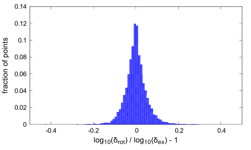
Figure 1: Correlation plot based on $10^{4}$ points for the process $u\bar{d}\to Wb\bar{b}g$ with massive bottom quarks

In the following, we will employ the rotation test as the standard method to estimate the precision of the finite part of each renormalized virtual matrix elements. If we call $\delta_{0}$ the error at any given phase space point and calculate it according to Eq. (36), we can define the precision of the finite part as $P_{0}=\log_{10}(\delta_{0})$. Concerning the precision of the double and single poles, $P_{-2}=\log_{10}(\delta_{-2})$ and $P_{-1}=\log_{10}(\delta_{-1})$, we employ the fact that the values of the pole coefficients, after renormalization, are solely due to infrared (IR) divergencies, whose expressions are well known [100]. $\delta_{-2}$ and $\delta_{-1}$ are defined using formula in Eq. (35), in which the exact values are provided by the reconstructed IR poles, which is automatically evaluated by GoSam.

In order to assess the level of precision of the results obtained with Ninja within GoSam, in Figs. 2 and 3, we plot the distributions of $P_{-2}$ (precision of the double pole), $P_{-1}$ (single pole) and $P_{0}$ (finite part) for two challenging virtual amplitudes with massive internal and external particles, namely $gg\to t\bar{t}Hg$ ($t\bar{t}Hj$) and $u\bar{u}\to Hu\bar{u}gg$ ($Hjjjj$) in VBF. By selecting an upper bound on the value of $P_{0}$, we can set a rejection criterium for phase space points in which the quality of the calculated scattering amplitudes falls below the requested precision. This also allows to estimate the percentage of points which would be discarded (or redirected to the rescue system). This value, as expected by analyzing the shape of the various distributions, is strongly process dependent and should be selected according to the particular phenomenological analysis at hand. As a benchmark value, in Ref. [9], the threshold for rejection was set to $P_{0}=-3$. In a similar fashion, in Table 1, we provide the percentages of bad points, which are points whose precision falls below the threshold, for increasing values of the rejection threshold.

The two plots are built using a set of $5\cdot 10^{4}$ and $1\cdot 10^{5}$ phase space points, respectively for $gg\to t\bar{t}Hg$ and $u\bar{u}\to Hu\bar{u}gg$ (VBF). No cuts have been introduced in the selection of the points, which are randomly distributed over the whole available phase space for the outgoing particles, and are generated using rambo.

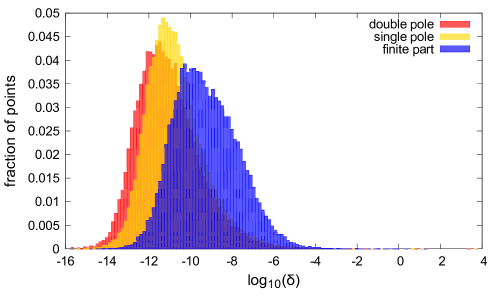
Figure 2: Precision Plot for $gg\to t\bar{t}Hg$: the distributions are obtained using $5\cdot 10^{4}$ randomly distributed phase space points.

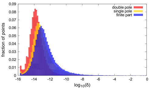
Figure 3: Precision plot for $u\bar{u}\to Hu\bar{u}gg$ in VBF: the distributions are obtained using $10^{5}$ randomly distributed phase space points.

$P_{0}$	$u\bar{u}\to Hu\bar{u}gg$	$gg\to t\bar{t}Hg$
$-3$	0.02%	0.06%
$-4$	0.04%	0.16%
$-5$	0.08%	0.56%

Table 1: Percentage of bad points as a function of the rejection threshold $P_{0}$.

The use of the novel algorithm implemented in Ninja  yields significant improvements both in the accuracy of results and in reduction of the computational time, due to a more efficient reduction and less frequent calls to the rescue system.

These features make GoSam+Ninja an extremely competitive framework for massive, as well as massless, calculations. The new library has been recently used in the evaluation of NLO QCD corrections to $pp\to t{\bar{t}}Hj$ [45].

5 Applications to Massive Amplitudes

In order to demonstrate the performances of the new reduction algorithm, we apply GoSam+Ninja to a collection of processes involving six, seven and eight external particles. We choose processes where massive particles appear in the products of the reactions or run in the loop. We list them in Table 2, and give the details of their calculations in the following subsections: for each process we provide results for a phase space point and a detailed list of the input parameters employed. While some of the considered processes have already been studied in the literature, the virtual NLO QCD contributions to $pp\to Wb{\bar{b}}+n$ jets ($n=1,2$), $pp\to Zb{\bar{b}}j$, $pp\to Zt{\bar{t}}j$, $pp\to VVVj$ (with $V=W,Z$), $pp\to ZZZZ$, and $pp\to H+n$ jets ($n=4,5$) in VBF are presented in this paper for the first time. When occurring in the final state, the bottom quark is treated as massive.

For calculation which were already performed with previous versions of the GoSam framework, we observe that the new reduction technique yields a significant net gain both in computing time and in accuracy. A paradigmatic example is represented by $gg\to Hggg$, whose evaluation per ps-point required approximately 20 seconds, as reported in [44], while now can be computed in less than 10 seconds.

In the following, for each of the considered scattering amplitudes, we provide a benchmark phase space point for the most involved subprocesses and, when possible, a comparison with results available in the literature. The coefficients $a_{i}$ are which appear in the various tables are defined as follows:

$$\frac{a_{-2}}{\epsilon^{2}}+\frac{a_{-1}}{\epsilon}+a_{0}\equiv\frac{2\mathfrak{Re}\left\{\mathcal{M}^{\mbox{\tiny tree-level}\ast}\mathcal{M}^{\mbox{\tiny one-loop}}\right\}}{(\alpha_{s}/2\pi)\left|\mathcal{M}^{\mbox{\tiny tree-level}}\right|^{2}}\,,$$

where the finite part $a_{0}$ is computed in the dimensional reduction scheme if not stated otherwise. The reconstruction of the renormalized pole can be checked against the value of $a_{-1}$ and $a_{-2}$ obtained by the universal singular behavior of the dimensionally regularized one-loop amplitudes [100], while the precision of the finite parts is estimated by re-evaluating the amplitudes for a set of momenta rotated by an arbitrary angle about the axis of collision, as described in Section 4. The accuracy of the results obtained with GoSam+Ninja is indicated by the underlined digits.

Benchmarks: GoSam + Ninja
Process		# NLO diagrams	ms/event
$W+3\,j$	${d}{\bar{u}}\rightarrow{\bar{\nu}_{e}}{e^{-}}{g}{g}{g}$	1 411	226
$Z+3\,j$	${d}{\bar{d}}\rightarrow{e^{+}}{e^{-}}{g}{g}{g}$	2 928	1 911
$Z\,Z\,Z+1\,j$	${u}{\bar{u}}\rightarrow{Z}{Z}{Z}{g}$	915	*12 000
${W}\,{W}\,{Z}+1\,j$	${u}{\bar{u}}\rightarrow{W^{+}}{W^{-}}{Z}{g}$	779	*7 050
${W}\,{Z}\,{Z}+1\,j$	${u}{\bar{d}}\rightarrow{W^{+}}{Z}{Z}{g}$	756	*3 300
${W}\,{W}\,{W}+1\,j$	${u}{\bar{d}}\rightarrow{W^{+}}{W^{-}}{W^{+}}{g}$	569	*1 800
$Z\,Z\,Z\,Z$	${u}\,{\bar{u}}\rightarrow{Z}\,{Z}\,{Z}\,{Z}$	408	*1 070
$W\,W\,W\,W$	${u}{\bar{u}}\rightarrow{W^{+}}{W^{-}}{W^{+}}{W^{-}}$	496	*1 350
$t\bar{t}b\bar{b}\,(m_{b}\neq 0)$	$\vphantom{e^{+}}d\bar{d}\rightarrow t\bar{t}b\bar{b}$	275	178
	$\vphantom{e^{+}}gg\rightarrow t\bar{t}b\bar{b}$	1 530	5 685
$t\bar{t}+2\,j$	$\vphantom{e^{+}}gg\rightarrow t\bar{t}gg$	4 700	13 827
$\vphantom{e^{+}}Z\,b\,\bar{b}+1\,j\,(m_{b}\neq 0)$	$\vphantom{e^{+}}d{u}{g}\rightarrow{u}{e^{+}}{e^{-}}{b}{\bar{b}}$	708	*1 070
$\vphantom{e^{+}}W\,b\,\bar{b}+1\,j\,(m_{b}\neq 0)$	$\vphantom{e^{+}}u\bar{d}\rightarrow e^{+}\nu_{e}b\bar{b}g$	312	67
$\vphantom{e^{+}}W\,b\,\bar{b}+2\,j\,(m_{b}\neq 0)$	${u}{\bar{d}}\rightarrow{e^{+}}{\nu_{e}}{b}{\bar{b}}{s}{\bar{s}}$	648	181
	${u}{\bar{d}}\rightarrow{e^{+}}{\nu_{e}}{b}{\bar{b}}{d}{\bar{d}}$	1 220	895
	${u}{\bar{d}}\rightarrow{e^{+}}{\nu_{e}}{b}{\bar{b}}{g}{g}$	3 923	5387
$\vphantom{e^{+}}W\,W\,b\,\bar{b}\,(m_{b}\neq 0)$	${d}{\bar{d}}\rightarrow{\nu_{e}}{e^{+}}{\bar{\nu}_{\mu}}{\mu^{-}}{b}{\bar{b}}$	292	115
	${g}{g}\rightarrow{\nu_{e}}{e^{+}}{\bar{\nu}_{\mu}}{\mu^{-}}{b}{\bar{b}}$	1 068	*5 300
$\vphantom{e^{+}}W\,W\,b\,\bar{b}+1\,j\,(m_{b}=0)$	${u}{\bar{u}}\rightarrow{\nu_{e}}{e^{+}}{\bar{\nu}_{\mu}}{\mu^{-}}{b}{\bar{b}}{g}$	3 612	*2 000
$H+3\,j$ in GF	$\vphantom{e^{+}}gg\rightarrow Hggg$	9 325	8 961
$\vphantom{e^{+}}{t}\,{\bar{t}}\,Z\,+1\,j$	${u}{\bar{u}}\rightarrow{t}{\bar{t}}{e^{+}}{e^{-}}{g}$	1408	1 220
	${g}{g}\rightarrow{t}{\bar{t}}{e^{+}}{e^{-}}{g}$	4230	19 560
$t\,\bar{t}\,H+1\,j$	$\vphantom{e^{+}}gg\rightarrow t\bar{t}Hg$	1 517	1 505
$H+3\,j$ in VBF	$\vphantom{e^{+}}{u}{\bar{u}}\rightarrow H{g}u\bar{u}$	432	101
$H+4\,j$ in VBF	$\vphantom{e^{+}}{u}{\bar{u}}\rightarrow H{g}{g}u\bar{u}$	1 176	669
$H+5\,j$ in VBF	$\vphantom{e^{+}}{u}{\bar{u}}\rightarrow H{g}{g}{g}u\bar{u}$	15 036	29 200

Table 2: A summary of results obtained with GoSam+Ninja. Timings refer to full color- and helicity-summed amplitudes, using an Intel Core i7 CPU @ 3.40GHz, compiled with ifort. The timings indicated with an (*) are obtained with an Intel(R) Xeon(R) CPU E5-2650 0 @ 2.00GHz, compiled with gfortran.

5.1 $p\,p\rightarrow W+3$ jets

Partonic process: ${d}{\bar{u}}\rightarrow{\bar{\nu}_{e}}{e^{-}}{g}{g}{g}$

The finite part for this process is given in the conventional dimensional regularization (CDR) scheme and was compared to the new version of NJet [16]. We also find agreement in the phase space point given by the BlackHat Collaboration [22].

particle	$E$	$p_{x}$	$p_{y}$	$p_{z}$
$p_{1}$	500.0000000000000000	0.0000000000000000	0.0000000000000000	500.0000000000000000
$p_{2}$	500.0000000000000000	0.0000000000000000	0.0000000000000000	-500.0000000000000000
$p_{3}$	414.1300683745429865	232.1455649459389861	332.7544367808189918	-82.9857518524426041
$p_{4}$	91.8751521026383955	-43.3570226791010995	-24.0058236140056991	77.3623460793434958
$p_{5}$	86.3540681437814044	-15.2133893202618005	37.6335512949163018	-76.2187226821854011
$p_{6}$	280.1181818093759830	-83.1261116505822031	-263.2038567586509998	47.7490851160265990
$p_{7}$	127.5225295696610033	-90.4490412959934957	-83.1783077030789002	34.0930433392580028

parameter	value
${m_{W}}$	80.419 GeV
${w_{W}}$	2.0476 GeV
${N_{f}}$	5
$\mu$	1000.0 GeV

	${d}{\bar{u}}\rightarrow{\bar{\nu}_{e}}{e^{-}}{g}{g}{g}$	Ref. [16]
$a_{0}$	-91.1772093904611438	-91.17720939055536
$a_{-1}$	-57.6891244440692361	-57.68912444409629
$a_{-2}$	-11.6666666666668277	-11.66666666666660

Table 3: Benchmark point for the subprocess $d(p_{1})\bar{u}(p_{2})\rightarrow\bar{\nu}_{e}(p_{3})e^{-}(p_{4})g(p_{5})g(p_{6})g(p_{7})$.

5.2 $p\,p\rightarrow Z+3$ jets

Partonic process: ${d}{\bar{d}}\rightarrow{e^{+}}{e^{-}}{g}{g}{g}$

The finite part for this process is given in CDR and was compared to the new version of NJet [16]. We also find agreement in the phase space point given by the BlackHat Collaboration [25].

particle	$E$	$p_{x}$	$p_{y}$	$p_{z}$
$p_{1}$	500.0000000000000000	0.0000000000000000	0.0000000000000000	500.0000000000000000
$p_{2}$	500.0000000000000000	0.0000000000000000	0.0000000000000000	-500.0000000000000000
$p_{3}$	414.1300683745429865	232.1455649459389861	332.7544367808189918	-82.9857518524426041
$p_{4}$	91.8751521026383955	-43.3570226791010995	-24.0058236140056991	77.3623460793434958
$p_{5}$	86.3540681437814044	-15.2133893202618005	37.6335512949163018	-76.2187226821854011
$p_{6}$	280.1181818093759830	-83.1261116505822031	-263.2038567586509998	47.7490851160265990
$p_{7}$	127.5225295696610033	-90.4490412959934957	-83.1783077030789002	34.0930433392580028

parameter	value
${m_{W}}$	80.419 GeV
${m_{Z}}$	91.188 GeV
${w_{Z}}$	2.4414 GeV
${N_{f}}$	5
$\mu$	1000.0 GeV

	${d}{\bar{d}}\rightarrow{e^{+}}{e^{-}}{g}{g}{g}$	Ref. [16]
$a_{0}$	-91.0463291277814761	-91.04632919538757
$a_{-1}$	-57.6876717480941892	-57.68767174883881
$a_{-2}$	-11.6666666666669485	-11.66666666666667

Table 4: Benchmark point for the subprocess $d(p_{1})\bar{d}(p_{2})\rightarrow e^{+}(p_{3})e^{-}(p_{4})g(p_{5})g(p_{6})g(p_{7})$.

5.3 ${p}\,{p}\rightarrow{Z}\,{Z}\,{Z}+1$ jet

Partonic process: ${u}{\bar{u}}\rightarrow{Z}{Z}{Z}{g}$

particle	$E$	$p_{x}$	$p_{y}$	$p_{z}$
$p_{1}$	250.0000000000000000	0.0000000000000000	0.0000000000000000	250.0000000000000000
$p_{2}$	250.0000000000000000	0.0000000000000000	0.0000000000000000	-250.0000000000000000
$p_{3}$	98.2984277476074197	25.7992145382080409	-12.3240263933454042	23.0200218627010820
$p_{4}$	178.4558180449861595	-120.4664227955374400	-73.7638561773535599	-59.8166791207833768
$p_{5}$	142.0905125919531145	50.7287365223860434	91.2424257480069656	-31.2402050144644221
$p_{6}$	81.1552416154533205	43.9384717349430645	-5.1545431773078745	68.0368622725466565

parameter	value
${m_{W}}$	80.376 GeV
${m_{Z}}$	91.1876 GeV
${N_{f}}$	5
$\mu$	500.0 GeV

	${u}{\bar{u}}\rightarrow{Z}{Z}{Z}{g}$
$a_{0}$	-18.2274687669522883
$a_{-1}$	-22.3832348831861125
$a_{-2}$	-5.6666666666670755

Table 5: Benchmark point for the subprocess $u(p_{1})\bar{u}(p_{2})\rightarrow Z(p_{3})Z(p_{4})Z(p_{5})g(p_{6})$.

5.4 ${p}\,{p}\rightarrow{W}\,{W}\,{Z}+1$ jet

Partonic process: ${u}{\bar{u}}\rightarrow{W^{+}}{W^{-}}{Z}{g}$

particle	$E$	$p_{x}$	$p_{y}$	$p_{z}$
$p_{1}$	250.0000000000000000	0.0000000000000000	0.0000000000000000	250.0000000000000000
$p_{2}$	250.0000000000000000	0.0000000000000000	0.0000000000000000	-250.0000000000000000
$p_{3}$	89.1058761118447791	27.0348198946258513	-12.9142626969235721	24.1225229592474193
$p_{4}$	179.7207629659015140	-126.2359378733789299	-77.2966387614043384	-62.6814876216509802
$p_{5}$	146.1313400758695593	53.1582949292336409	95.6123118862003167	-32.7363964816230890
$p_{6}$	85.0420208463841476	46.0428230495191357	-5.4014104278722739	71.2953611440265860

parameter	value
${m_{W}}$	80.376 GeV
${m_{Z}}$	91.1876 GeV
${N_{f}}$	5
$\mu$	500.0 GeV

	${u}{\bar{u}}\rightarrow{W^{+}}{W^{-}}{Z}{g}$
$a_{0}$	-18.0050305906438837
$a_{-1}$	-22.1025452011781987
$a_{-2}$	-5.6666666666666661

Table 6: Benchmark point for the subprocess $u(p_{1})\bar{u}(p_{2})\rightarrow W^{+}(p_{3})W^{-}(p_{4})Z(p_{5})g(p_{6})$.

5.5 ${p}\,{p}\rightarrow{W}\,{Z}\,{Z}+1$ jet

Partonic process: ${u}{\bar{d}}\rightarrow{W^{+}}{Z}{Z}{g}$

particle	$E$	$p_{x}$	$p_{y}$	$p_{z}$
$p_{1}$	250.0000000000000000	0.0000000000000000	0.0000000000000000	250.0000000000000000
$p_{2}$	250.0000000000000000	0.0000000000000000	0.0000000000000000	-250.0000000000000000
$p_{3}$	88.8514948513947331	26.6180234830689777	-12.7151632255396141	23.7506254934495686
$p_{4}$	182.6577199093957518	-124.2897556491134168	-76.1049547854528043	-61.7151257515301381
$p_{5}$	144.7598590943426586	52.3387523298249846	94.1382547757718982	-32.2316987387113372
$p_{6}$	83.7309261448668849	45.3329798362191525	-5.3181367647793465	70.1961989967918498

parameter	value
${m_{W}}$	80.376 GeV
${m_{Z}}$	91.1876 GeV
${N_{f}}$	5
$\mu$	500.0 GeV

	${u}{\bar{d}}\rightarrow{W^{+}}{Z}{Z}{g}$
$a_{0}$	-16.6719638614981740
$a_{-1}$	-22.1957678011010735
$a_{-2}$	-5.6666666666670213

Table 7: Benchmark point for the subprocess $u(p_{1})\bar{d}(p_{2})\rightarrow W^{+}(p_{3})Z(p_{4})Z(p_{5})g(p_{6})$.

5.6 ${p}\,{p}\rightarrow{W}\,{W}\,{W}+1$ jet

Partonic process: ${u}{\bar{d}}\rightarrow{W^{+}}{W^{-}}{W^{+}}{g}$

particle	$E$	$p_{x}$	$p_{y}$	$p_{z}$
$p_{1}$	250.0000000000000000	0.0000000000000000	0.0000000000000000	250.0000000000000000
$p_{2}$	250.0000000000000000	0.0000000000000000	0.0000000000000000	-250.0000000000000000
$p_{3}$	89.4258007278425993	27.5517039326065500	-13.1611730250244197	24.5837262194154818
$p_{4}$	182.4747913234621421	-128.6494675939613614	-78.7744883983191500	-63.8799073098456347
$p_{5}$	141.4314519821789986	54.1746388235997784	97.4403424793774207	-33.3622900835894285
$p_{6}$	86.6679559665162316	46.9231248377547274	-5.5046810560337240	72.6584711740195104

parameter	value
${m_{W}}$	80.376 GeV
${m_{Z}}$	91.1876 GeV
${N_{f}}$	5
$\mu$	500.0 GeV

	${u}{\bar{d}}\rightarrow{W^{+}}{W^{-}}{W^{+}}{g}$
$a_{0}$	-15.8859769338002099
$a_{-1}$	-21.9889128719035618
$a_{-2}$	-5.6666666666864467

Table 8: Benchmark point for the subprocess $u(p_{1})\bar{d}(p_{2})\rightarrow W^{+}(p_{3})W^{-}(p_{4})W^{+}(p_{5})g(p_{6})$.

5.7 ${p}\,{p}\rightarrow{Z}\,{Z}\,{Z}\,{Z}$

Partonic process: ${u}\,{\bar{u}}\rightarrow{Z}\,{Z}\,{Z}\,{Z}$

particle	$E$	$p_{x}$	$p_{y}$	$p_{z}$
$p_{1}$	250.0000000000000000	0.0000000000000000	0.0000000000000000	250.0000000000000000
$p_{2}$	250.0000000000000000	0.0000000000000000	0.0000000000000000	-250.0000000000000000
$p_{3}$	96.3863867610220666	21.9480082963376795	-10.4843437432888980	19.5836826767025762
$p_{4}$	159.2027435644542095	-102.4836644941604078	-62.7526750844588079	-50.8874782857443790
$p_{5}$	130.0351856078737001	43.1561483551038094	77.6221118797800074	-26.5767889104262487
$p_{6}$	114.3756840666499812	37.3795078427186667	-4.3850930520321931	57.8805845194680018

parameter	value
${m_{W}}$	80.376 GeV
${m_{Z}}$	91.1876 GeV
${N_{f}}$	5
$\mu$	500.0 GeV

	${u}{\bar{u}}\rightarrow{Z}{Z}{Z}{Z}$
$a_{0}$	10.0010268560339206
$a_{-1}$	-3.9999999999613696
$a_{-2}$	-2.6666666666665884

Table 9: Benchmark point for the subprocess $u(p_{1})\bar{u}(p_{2})\rightarrow Z(p_{3})Z(p_{4})Z(p_{5})Z(p_{6})$.

5.8 ${p}\,{p}\rightarrow{W}\,{W}\,{W}\,{W}$

Partonic process: ${u}{\bar{u}}\rightarrow{W^{+}}{W^{-}}{W^{+}}{W^{-}}$

particle	$E$	$p_{x}$	$p_{y}$	$p_{z}$
$p_{1}$	250.0000000000000000	0.0000000000000000	0.0000000000000000	250.0000000000000000
$p_{2}$	250.0000000000000000	0.0000000000000000	0.0000000000000000	-250.0000000000000000
$p_{3}$	87.7920438094441096	24.8207950462383629	-11.8566452013738353	22.1470015595954024
$p_{4}$	168.0494737136866092	-115.8978071108833205	-70.9664068759461202	-57.5481680112689915
$p_{5}$	132.1031656516532848	48.8048800986569518	87.7821123452778238	-30.0554392738635485
$p_{6}$	112.0553168252159821	42.2721319659877182	-4.9590602679577351	65.4566057255370879

parameter	value
${m_{W}}$	80.376 GeV
${m_{Z}}$	91.1876 GeV
${N_{f}}$	5
$\mu$	500.0 GeV

	${u}{\bar{u}}\rightarrow{W^{+}}{W^{-}}{W^{+}}{W^{-}}$
$a_{0}$	7.8556327396245011
$a_{-1}$	-3.9999999999981126
$a_{-2}$	-2.6666666666669747

Table 10: Benchmark point for the subprocess $u(p_{1})\bar{u}(p_{2})\rightarrow W^{+}(p_{3})W^{-}(p_{4})W^{+}(p_{5})W^{-}(p_{6})$.

5.9 $p\,p\rightarrow t\,\bar{t}\,b\,\bar{b}$

Partonic process: ${d}{\bar{d}}\rightarrow{t}{\bar{t}}{b}{\bar{b}}$

particle	$E$	$p_{x}$	$p_{y}$	$p_{z}$
$p_{1}$	250.0000000000000000	0.0000000000000000	0.0000000000000000	250.0000000000000000
$p_{2}$	250.0000000000000000	0.0000000000000000	0.0000000000000000	-250.0000000000000000
$p_{3}$	213.1527786548405459	-26.8458616570582116	-117.8628562648380296	-38.8884799556846303
$p_{4}$	220.5509350311838546	61.9684848664477599	92.5635212096267281	83.2176445698946168
$p_{5}$	42.2714703981682263	-16.8075489037092431	24.9923105627744704	-29.3620149548096769
$p_{6}$	24.0248159158073982	-18.3150743056803300	0.3070244924368429	-14.9671496594002438

parameter	value
${m_{t}}$	171.2 GeV
${m_{b}}$	4.2 GeV
${N_{f}}$	4
$\mu$	500.0 GeV

	${d}{\bar{d}}\rightarrow{t}{\bar{t}}{b}{\bar{b}}$
$a_{0}$	154.6475673006605973
$a_{-1}$	2.7409050914577211
$a_{-2}$	-2.6666666666666683

Table 11: Benchmark point for the subprocess $d(p_{1})\bar{d}(p_{2})\rightarrow t(p_{3})\bar{t}(p_{4})b(p_{5})\bar{b}(p_{6})$.

Partonic process: ${g}{g}\rightarrow{t}{\bar{t}}{b}{\bar{b}}$

particle	$E$	$p_{x}$	$p_{y}$	$p_{z}$
$p_{1}$	250.0000000000000000	0.0000000000000000	0.0000000000000000	250.0000000000000000
$p_{2}$	250.0000000000000000	0.0000000000000000	0.0000000000000000	-250.0000000000000000
$p_{3}$	194.0670578462199387	-60.6594324624948058	-47.3641590248774236	-49.2915067154802884
$p_{4}$	172.4499944124030151	-15.6689752760792977	-7.1446619651393677	-11.5324581958636152
$p_{5}$	61.9093840678718479	12.0715208460656545	23.6785835371366993	55.7560301833003820
$p_{6}$	71.5735636735052054	64.2568868925084331	30.8302374528801408	5.0679347280435243

parameter	value
${m_{t}}$	171.2 GeV
${m_{b}}$	4.2 GeV
${N_{f}}$	4
$\mu$	500.0 GeV

	${g}{g}\rightarrow{t}{\bar{t}}{b}{\bar{b}}$
$a_{0}$	165.1250038552732349
$a_{-1}$	-3.4472725930136989
$a_{-2}$	-6.0000000000001563

Table 12: Benchmark point for the subprocess $g(p_{1})g(p_{2})\rightarrow t(p_{3})\bar{t}(p_{4})b(p_{5})\bar{b}(p_{6})$.

5.10 $p\,p\rightarrow t\,\bar{t}+2$ jets

Partonic process: ${g}{g}\rightarrow{t}{\bar{t}}{g}{g}$

The finite part for this process is given in CDR and was compared with Ref. [29].

particle	$E$	$p_{x}$	$p_{y}$	$p_{z}$
$p_{1}$	2424.7465026975200999	0.0000000000000000	0.0000000000000000	2424.7465026975200999
$p_{2}$	2424.7465026975200999	0.0000000000000000	0.0000000000000000	-2424.7465026975200999
$p_{3}$	881.9042263139403985	-715.3340594013137661	-475.1625187999429158	101.1925816377931966
$p_{4}$	343.4841188963524132	-24.1478321960174789	-6.3283366075706340	295.5085181344487069
$p_{5}$	1673.4634600426329598	21.8782679485017297	1000.4115637957629588	1341.3344089052341133
$p_{6}$	1950.6412001421140303	717.6036236488295117	-518.9207083882492952	-1738.0355086774759457

parameter	value
${m_{t}}$	173.3 GeV
${N_{f}}$	5
$\mu$	173.3 GeV

	${g}{g}\rightarrow{t}{\bar{t}}{g}{g}$	Ref. [29]
$a_{0}$	-93.9825428068626394	-93.98254280655584
$a_{-1}$	47.0991735298819236	47.0991735300671
$a_{-2}$	-11.9999999999947171	-11.999999999999874

Table 13: Benchmark point for the subprocess $g(p_{1})g(p_{2})\rightarrow t(p_{3})\bar{t}(p_{4})g(p_{5})g(p_{6})$.

5.11 $p\,p\rightarrow Z\,b\,\bar{b}+1$ jet

Partonic process: ${u}{g}\rightarrow{u}{e^{+}}{e^{-}}{b}{\bar{b}}$

particle	$E$	$p_{x}$	$p_{y}$	$p_{z}$
$p_{1}$	250.0000000000000000	0.0000000000000000	0.0000000000000000	250.0000000000000000
$p_{2}$	250.0000000000000000	0.0000000000000000	0.0000000000000000	-250.0000000000000000
$p_{3}$	34.5908278264605187	21.2091909896352142	-9.4555401980608202	25.6376353599131122
$p_{4}$	166.7223525775519022	-156.7623134542972991	-48.7827423195217946	-29.0200617028515602
$p_{5}$	111.6942046513332798	30.9750523871488710	106.1302756897373314	-15.8904394000814051
$p_{6}$	84.2714416207739418	35.0918815486497024	1.4231216042880672	76.4890217424595988
$p_{7}$	102.7211733238803646	69.4861885288632521	-49.3151147764427051	-57.2161559994397777

parameter	value
${m_{W}}$	80.376 GeV
${w_{W}}$	2.124 GeV
${m_{b}}$	4.2 GeV
${N_{f}}$	4
$\mu$	500.0 GeV

	${u}{g}\rightarrow{u}{e^{+}}{e^{-}}{b}{\bar{b}}$
$a_{0}$	145.3708954680396630
$a_{-1}$	-8.3679512693708471
$a_{-2}$	-5.6666666666675392

Table 14: Benchmark point for the subprocess $u(p_{1})g(p_{2})\rightarrow u(p_{3})e^{+}(p_{4})e^{-}(p_{5})b(p_{6})\bar{b}(p_{7})$.

5.12 $p\,p\rightarrow W\,b\,\bar{b}+1$ jet

Partonic process: ${u}{\bar{d}}\rightarrow{e^{+}}{\nu_{e}}{b}{\bar{b}}{g}$

particle	$E$	$p_{x}$	$p_{y}$	$p_{z}$
$p_{1}$	250.0000000000000000	0.0000000000000000	0.0000000000000000	250.0000000000000000
$p_{2}$	250.0000000000000000	0.0000000000000000	0.0000000000000000	-250.0000000000000000
$p_{3}$	93.4300963683620580	-16.6492363753179085	-37.4579803162897420	-83.9576413803095818
$p_{4}$	119.9994454272237192	4.7053605726301706	-100.6826015733804809	65.1209660949429150
$p_{5}$	57.9859979994296282	9.1381348721238638	-4.6735873988293006	56.9156220722767259
$p_{6}$	104.9559149323387999	87.3260122226470514	54.3049824548373437	-20.5728109201014071
$p_{7}$	123.6285452726457805	-84.5202712920831658	88.5091868336622554	-17.5061358668087337

parameter	value
${m_{W}}$	80.376 GeV
${w_{W}}$	2.124 GeV
${m_{b}}$	4.2 GeV
${N_{f}}$	4
$\mu$	500.0 GeV

	${u}{\bar{d}}\rightarrow{e^{+}}{\nu_{e}}{b}{\bar{b}}{g}$
$a_{0}$	129.9538554864771243
$a_{-1}$	-5.3385683701189715
$a_{-2}$	-5.6666666666668695

Table 15: Benchmark point for the subprocess $u(p_{1})\bar{d}(p_{2})\rightarrow e^{+}(p_{3})\nu_{e}(p_{4})b(p_{5})\bar{b}(p_{6})g(p_{7})$.

5.13 $p\,p\rightarrow W\,b\,\bar{b}+2$ jets

Partonic process: ${u}{\bar{d}}\rightarrow{e^{+}}{\nu_{e}}{b}{\bar{b}}{d}{\bar{d}}$

particle	$E$	$p_{x}$	$p_{y}$	$p_{z}$
$p_{1}$	250.0000000000000000	0.0000000000000000	0.0000000000000000	250.0000000000000000
$p_{2}$	250.0000000000000000	0.0000000000000000	0.0000000000000000	-250.0000000000000000
$p_{3}$	125.6965187314100234	-17.0943040170214537	-113.3597903541534748	51.5456838370753374
$p_{4}$	72.1993434263444129	25.0205029393394440	42.4573677065765622	52.7644913865970722
$p_{5}$	130.5494441454287085	-59.2470822889473183	116.2307891878907924	-2.3883575291830641
$p_{6}$	52.9433261580396106	45.1283306603629413	-14.5296908876010313	-23.1878769876905828
$p_{7}$	99.1517346871049057	-5.9484899951818377	-31.1690273964595583	-93.9370730297576273
$p_{8}$	19.4596328516722785	12.1410427014482281	0.3703517437466808	15.2031323229588882

parameter	value
${m_{W}}$	80.376 GeV
${w_{W}}$	2.124 GeV
${m_{b}}$	4.2 GeV
${N_{f}}$	4
$\mu$	500.0 GeV

	${u}{\bar{d}}\rightarrow{e^{+}}{\nu_{e}}{b}{\bar{b}}{d}{\bar{d}}$
$a_{0}$	148.2499564138260837
$a_{-1}$	-7.7272995122163879
$a_{-2}$	-5.3333333333331892

Table 16: Benchmark point for the subprocess $u(p_{1})\bar{d}(p_{2})\rightarrow e^{+}(p_{3})\nu_{e}(p_{4})b(p_{5})\bar{b}(p_{6})d(p_{7})\bar{d}(p_{8})$.

Partonic process: ${u}{\bar{d}}\rightarrow{e^{+}}{\nu_{e}}{b}{\bar{b}}{s}{\bar{s}}$

particle	$E$	$p_{x}$	$p_{y}$	$p_{z}$
$p_{1}$	250.0000000000000000	0.0000000000000000	0.0000000000000000	250.0000000000000000
$p_{2}$	250.0000000000000000	0.0000000000000000	0.0000000000000000	-250.0000000000000000
$p_{3}$	1.8312125180161738	1.2481975210878733	-0.3016228634824342	-1.3055136470806736
$p_{4}$	132.0663362603577298	-16.6607423420677527	94.8432229336175965	-90.3808602603960196
$p_{5}$	121.6089450080674226	-63.6699664483805989	-102.6429343577717077	13.4780898076629523
$p_{6}$	51.8272368161295987	-33.3143054988286877	-36.6615737768635270	-14.6461098360448521
$p_{7}$	124.2305315458477253	116.2047315474863467	-2.8413585495376918	43.8361952698163435
$p_{8}$	68.4357378515813224	-3.8079147792972257	47.6042666140377335	49.0181986660422169

parameter	value
${m_{W}}$	80.376 GeV
${w_{W}}$	2.124 GeV
${m_{b}}$	4.2 GeV
${N_{f}}$	4
$\mu$	500.0 GeV

	${u}{\bar{d}}\rightarrow{e^{+}}{\nu_{e}}{b}{\bar{b}}{s}{\bar{s}}$
$a_{0}$	161.1656361677729592
$a_{-1}$	-1.3276262260753209
$a_{-2}$	-5.3333333333332735

Table 17: Benchmark point for the subprocess $u(p_{1})\bar{d}(p_{2})\rightarrow e^{+}(p_{3})\nu_{e}(p_{4})b(p_{5})\bar{b}(p_{6})s(p_{7})\bar{s}(p_{8})$.

Partonic process: ${u}{\bar{d}}\rightarrow{e^{+}}{\nu_{e}}{b}{\bar{b}}{g}{g}$

particle	$E$	$p_{x}$	$p_{y}$	$p_{z}$
$p_{1}$	250.0000000000000000	0.0000000000000000	0.0000000000000000	250.0000000000000000
$p_{2}$	250.0000000000000000	0.0000000000000000	0.0000000000000000	-250.0000000000000000
$p_{3}$	118.4116290336479551	49.7302976872290259	-105.1432905838027665	-22.2058512007951201
$p_{4}$	9.9876328289379046	7.4336546931814604	4.5250271451401858	4.9007873616352553
$p_{5}$	113.2724870353399353	-8.8682847027615033	110.4231681698792471	23.2614225044082019
$p_{6}$	50.3648230617062964	-38.8899369624844553	-31.0689344437605435	-6.4241355543198972
$p_{7}$	105.2876197360011901	-28.2113391151385819	10.7916624062129962	100.8620009592996638
$p_{8}$	102.6758083043666687	18.8056083999740657	10.4723673063308507	-100.3942240702281055

parameter	value
${m_{W}}$	80.376 GeV
${w_{W}}$	2.124 GeV
${m_{b}}$	4.2 GeV
${N_{f}}$	4
$\mu$	500.0 GeV

	${u}{\bar{d}}\rightarrow{e^{+}}{\nu_{e}}{b}{\bar{b}}{g}{g}$
$a_{0}$	64.8935770569783301
$a_{-1}$	-35.9610562256753425
$a_{-2}$	-8.6666666666670285

Table 18: Benchmark point for the subprocess $u(p_{1})\bar{d}(p_{2})\rightarrow e^{+}(p_{3})\nu_{e}(p_{4})b(p_{5})\bar{b}(p_{6})g(p_{7})g(p_{8})$.

5.14 ${p}\,{p}\rightarrow{W}\,{W}\,{b}\,{\bar{b}}$

Partonic process: ${d}{\bar{d}}\rightarrow{\nu_{e}}{e^{+}}{\bar{\nu}_{\mu}}{\mu^{-}}{b}{\bar{b}}$

particle	$E$	$p_{x}$	$p_{y}$	$p_{z}$
$p_{1}$	250.0000000000000000	0.0000000000000000	0.0000000000000000	250.0000000000000000
$p_{2}$	250.0000000000000000	0.0000000000000000	0.0000000000000000	-250.0000000000000000
$p_{3}$	25.6649135887983881	15.7119189648809563	-7.6256852614994211	18.8061776088085644
$p_{4}$	154.5064489409292605	-136.9768135536888565	-46.2042967903236104	-54.5413446032057010
$p_{5}$	96.1603526761926730	22.3143342117606984	88.8440473781699325	-29.2509685474019605
$p_{6}$	61.0731578730670606	23.2528867537403734	2.3717946919774544	56.4234743714476039
$p_{7}$	93.6199892430268648	58.9397665353324101	-43.8226058551382351	-57.9028973600646211
$p_{8}$	68.9751376779857708	16.7579070879743455	6.4367458368138966	66.4655585304161036

parameter	value
${m_{W}}$	80.376 GeV
${m_{Z}}$	91.1876 GeV
${m_{t}}$	171.2 GeV
${m_{b}}$	4.2 GeV
${N_{f}}$	4
$\mu$	500.0 GeV

	${d}{\bar{d}}\rightarrow{\nu_{e}}{e^{+}}{\bar{\nu}_{\mu}}{\mu^{-}}{b}{\bar{b}}$
$a_{0}$	118.3990066409585751
$a_{-1}$	8.5574384926230991
$a_{-2}$	-2.6666666666666492

Table 19: Benchmark point for the subprocess $d(p_{1})\bar{d}(p_{2})\rightarrow\nu_{e}(p_{3})e^{+}(p_{4})\bar{\nu}_{\mu}(p_{5})\mu^{-}(p_{6})b(p_{7})\bar{b}(p_{8})$.

Partonic process: ${g}{g}\rightarrow{\nu_{e}}{e^{+}}{\bar{\nu}_{\mu}}{\mu^{-}}{b}{\bar{b}}$

particle	$E$	$p_{x}$	$p_{y}$	$p_{z}$
$p_{1}$	250.0000000000000000	0.0000000000000000	0.0000000000000000	250.0000000000000000
$p_{2}$	250.0000000000000000	0.0000000000000000	0.0000000000000000	-250.0000000000000000
$p_{3}$	25.6649135887983881	15.7119189648809563	-7.6256852614994211	18.8061776088085644
$p_{4}$	154.5064489409292605	-136.9768135536888565	-46.2042967903236104	-54.5413446032057010
$p_{5}$	96.1603526761926730	22.3143342117606984	88.8440473781699325	-29.2509685474019605
$p_{6}$	61.0731578730670606	23.2528867537403734	2.3717946919774544	56.4234743714476039
$p_{7}$	93.6199892430268648	58.9397665353324101	-43.8226058551382351	-57.9028973600646211
$p_{8}$	68.9751376779857708	16.7579070879743455	6.4367458368138966	66.4655585304161036

parameter	value
${m_{W}}$	80.376 GeV
${m_{Z}}$	91.1876 GeV
${m_{t}}$	171.2 GeV
${m_{b}}$	4.2 GeV
${N_{f}}$	4
$\mu$	500.0 GeV

	${g}{g}\rightarrow{\nu_{e}}{e^{+}}{\bar{\nu}_{\mu}}{\mu^{-}}{b}{\bar{b}}$
$a_{0}$	27.4387494492212056
$a_{-1}$	-7.9555523940773458
$a_{-2}$	-5.9999999999999885

Table 20: Benchmark point for the subprocess $g(p_{1})g(p_{2})\rightarrow\nu_{e}(p_{3})e^{+}(p_{4})\bar{\nu}_{\mu}(p_{5})\mu^{-}(p_{6})b(p_{7})\bar{b}(p_{8})$.

5.15 ${p}\,{p}\rightarrow{W}\,{W}\,{b}\,{\bar{b}}+1$ jet

Partonic process: ${u}{\bar{u}}\rightarrow{\nu_{e}}{e^{+}}{\bar{\nu}_{\mu}}{\mu^{-}}{b}{\bar{b}}{g}$

particle	$E$	$p_{x}$	$p_{y}$	$p_{z}$
$p_{1}$	250.0000000000000000	0.0000000000000000	0.0000000000000000	250.0000000000000000
$p_{2}$	250.0000000000000000	0.0000000000000000	0.0000000000000000	-250.0000000000000000
$p_{3}$	18.1435357791203664	10.6794732394995044	-3.3652659935279523	14.2762644514536543
$p_{4}$	132.6867460765342059	-121.1435093670056773	-5.2844663256145745	-53.8711159925087628
$p_{5}$	92.9820970636741606	17.2946496492191066	87.0024013115393018	-27.8773677719967203
$p_{6}$	46.6813566690488102	14.7875289839330328	9.6031823094958089	43.2233378690595345
$p_{7}$	69.5794003816978091	41.1619960772432023	-24.4397402957503331	-50.4943772185567497
$p_{8}$	53.6926389028252160	9.1521313351918430	14.4565277002773502	50.8934845655482206
$p_{9}$	86.2342251270994211	28.0677300819189206	-77.9726387064195876	23.8497740970007897

parameter	value
${m_{W}}$	80.376 GeV
${m_{Z}}$	91.1876 GeV
${m_{t}}$	171.2 GeV
${m_{b}}$	0.0 GeV
${N_{f}}$	5
$\mu^{2}$	500.0 GeV

	${u}{\bar{u}}\rightarrow{\nu_{e}}{e^{+}}{\bar{\nu}_{\mu}}{\mu^{-}}{b}{\bar{b}}{g}$
$a_{0}$	-38.5591246673060795
$a_{-1}$	-32.4828496060584442
$a_{-2}$	-8.3333333333334405

Table 21: Benchmark point for the subprocess $u(p_{1})\bar{u}(p_{2})\rightarrow\nu_{e}(p_{3})e^{+}(p_{4})\bar{\nu}_{\mu}(p_{5})\mu^{-}(p_{6})b(p_{7})\bar{b}(p_{8})g(p_{9})$.

5.16 $p\,p\rightarrow H+3$ jets

Partonic process: ${g}{g}\rightarrow{H}{g}{g}{g}$

particle	$E$	$p_{x}$	$p_{y}$	$p_{z}$
$p_{1}$	250.0000000000000000	0.0000000000000000	0.0000000000000000	250.0000000000000000
$p_{2}$	250.0000000000000000	0.0000000000000000	0.0000000000000000	-250.0000000000000000
$p_{3}$	144.2726812297522656	26.1871426153409317	-66.9976759414063139	3.8924965402436307
$p_{4}$	135.5632052379070274	5.8338195550562180	26.5129120011233681	-132.8172227574218596
$p_{5}$	75.6651361325424006	-19.2292152047334604	-65.8505932559228597	31.9241206051040152
$p_{6}$	144.4989773997982923	-12.7917469656637373	106.3353571962057913	97.0006056120742102

parameter	value
${m_{H}}$	125.0 GeV
${N_{f}}$	5
$\mu$	500.0 GeV

	${g}{g}\rightarrow{H}{g}{g}{g}$
$a_{0}$	23.4307927578718953
$a_{-1}$	-56.3734964424517315
$a_{-2}$	-15.0000000000008757

Table 22: Benchmark point for the subprocess $g(p_{1})g(p_{2})\rightarrow H(p_{3})g(p_{4})g(p_{5})g(p_{6})$.

5.17 $p\,p\rightarrow Z\,t\,\bar{t}+1$ jet

Partonic process: ${u}{\bar{u}}\rightarrow{t}{\bar{t}}{e^{+}}{e^{-}}{g}$

particle	$E$	$p_{x}$	$p_{y}$	$p_{z}$
$p_{1}$	250.0000000000000000	0.0000000000000000	0.0000000000000000	250.0000000000000000
$p_{2}$	250.0000000000000000	0.0000000000000000	0.0000000000000000	-250.0000000000000000
$p_{3}$	183.2414081421947287	-30.2337217736484156	32.1314578860740667	48.1815850690226029
$p_{4}$	199.0327070603159996	74.5268539046026035	-40.9270527537185629	-55.4554134393922311
$p_{5}$	70.1181125436057044	-63.0760999348447697	21.5315800178266556	21.7794946135846281
$p_{6}$	20.7607087314536756	-7.2430664321972609	-7.1983324871256098	-18.0756472939650585
$p_{7}$	26.8470635224299627	26.0260342360878454	-5.5376526630565506	3.5699810507501222

parameter	value
${m_{Z}}$	91.1876 GeV
${m_{t}}$	171.2 GeV
${N_{f}}$	5
$\mu$	500.0 GeV

	${u}{\bar{u}}\rightarrow{t}{\bar{t}}{e^{+}}{e^{-}}{g}$
$a_{0}$	-20.4367763710913373
$a_{-1}$	-25.9078542815554513
$a_{-2}$	-5.6666666665792098

Table 23: Benchmark point for the subprocess $u(p_{1})\bar{u}(p_{2})\rightarrow t(p_{3})\bar{t}(p_{4})e^{+}(p_{5})e^{-}(p_{6})g(p_{7})$.

Partonic process: ${g}{g}\rightarrow{t}{\bar{t}}{e^{+}}{e^{-}}{g}$

particle	$E$	$p_{x}$	$p_{y}$	$p_{z}$
$p_{1}$	250.0000000000000000	0.0000000000000000	0.0000000000000000	250.0000000000000000
$p_{2}$	250.0000000000000000	0.0000000000000000	0.0000000000000000	-250.0000000000000000
$p_{3}$	174.2203895522303014	-25.0977827305029138	-19.5610151031829993	5.5472629175473589
$p_{4}$	186.7123996976260685	-14.0800163072181022	56.3619207264196902	-46.6601246640355427
$p_{5}$	60.3016377245591073	38.1795332240129639	22.1553968884492853	41.0822241824339116
$p_{6}$	18.6184873501163182	5.2347824612577458	-1.6661313271933778	-17.7895792583830961
$p_{7}$	60.1470856754682259	-4.2365166475497116	-57.2901711844925998	17.8202168224373914

parameter	value
${m_{Z}}$	91.1876 GeV
${m_{t}}$	171.2 GeV
${N_{f}}$	5
$\mu$	500.0 GeV

	${g}{g}\rightarrow{t}{\bar{t}}{e^{+}}{e^{-}}{g}$
$a_{0}$	9.2826425323344441
$a_{-1}$	-26.2816094048822784
$a_{-2}$	-9.0000000000005702

Table 24: Benchmark point for the subprocess $g(p_{1})g(p_{2})\rightarrow t(p_{3})\bar{t}(p_{4})e^{+}(p_{5})e^{-}(p_{6})g(p_{7})$.

5.18 $p\,p\rightarrow H\,t\,\bar{t}+1$ jet

Partonic process: ${g}{g}\rightarrow{H}{t}{\bar{t}}{g}$

particle	$E$	$p_{x}$	$p_{y}$	$p_{z}$
$p_{1}$	250.0000000000000000	0.0000000000000000	0.0000000000000000	250.0000000000000000
$p_{2}$	250.0000000000000000	0.0000000000000000	0.0000000000000000	-250.0000000000000000
$p_{3}$	126.3747891763443505	6.8355633672742222	-3.2652801590882752	6.0992096455298030
$p_{4}$	177.2234233286846745	-31.9178657717747534	-19.5439094615872051	-15.8485716665707326
$p_{5}$	174.8995128490773538	13.4406996200208031	24.1748981179500326	-8.2771667589629576
$p_{6}$	21.5022746458936318	11.6416027844796517	-1.3657084972745175	18.0265287800038720

parameter	value
${m_{H}}$	126.0 GeV
${m_{t}}$	172.5 GeV
${N_{f}}$	5
$\mu$	500.0 GeV

	${g}{g}\rightarrow{H}{t}{\bar{t}}{g}$
$a_{0}$	-45.6979334407767297
$a_{-1}$	-35.9217497445515619
$a_{-2}$	-8.9999999999990887

Table 25: Benchmark point for the subprocess $g(p_{1})g(p_{2})\rightarrow H(p_{3})t(p_{4})\bar{t}(p_{5})g(p_{6})$.

5.19 $p\,p\rightarrow H+3$ jets (VBF)

Partonic process: ${u}{u}\rightarrow{g}{H}{u}{u}$ (VBF)

particle	$E$	$p_{x}$	$p_{y}$	$p_{z}$
$p_{1}$	250.0000000000000000	0.0000000000000000	0.0000000000000000	250.0000000000000000
$p_{2}$	250.0000000000000000	0.0000000000000000	0.0000000000000000	-250.0000000000000000
$p_{3}$	40.1603071333660182	-14.0012702315405289	0.4395613413056457	37.6380324509251736
$p_{4}$	127.7084583092647421	-23.4171446211731009	-10.8486559189339324	4.2888607196847408
$p_{5}$	145.0573545181100599	-109.8833468186949176	-94.5094823127907233	5.9366610719649477
$p_{6}$	187.0738800392591656	147.3017616714085705	104.9185768904190468	-47.8635542425748710

parameter	value
${m_{H}}$	125.0 GeV
${m_{Z}}$	91.1876 GeV
${w_{Z}}$	2.4952 GeV
${N_{f}}$	5
$\mu$	500.0 GeV

	${u}{u}\rightarrow{g}{H}{u}{u}$
$a_{0}$	-94.6818287259862359
$a_{-1}$	-40.8904107779583796
$a_{-2}$	-8.3333333333336821

Table 26: Benchmark point for the subprocess $u(p_{1})u(p_{2})\rightarrow g(p_{3})H(p_{4})u(p_{5})u(p_{6})$.

5.20 $p\,p\rightarrow H+4$ jets (VBF)

Partonic process: ${u}{u}\rightarrow{g}{g}{H}{u}{u}$ (VBF)

particle	$E$	$p_{x}$	$p_{y}$	$p_{z}$
$p_{1}$	250.0000000000000000	0.0000000000000000	0.0000000000000000	250.0000000000000000
$p_{2}$	250.0000000000000000	0.0000000000000000	0.0000000000000000	-250.0000000000000000
$p_{3}$	77.8540004794647871	-42.9509851388533761	6.0812524321357140	-64.6488718781321126
$p_{4}$	179.6868495846460405	66.2917119993839208	-68.8295351006103004	152.1685510599341171
$p_{5}$	140.8511015083574875	-29.7530986170501173	2.6554844463192953	-57.6344889901617350
$p_{6}$	81.8035523206006161	2.3404081739038114	78.3533883805051659	-23.3899591949725902
$p_{7}$	19.8044961069310155	4.0719635826157594	-18.2605901583498813	-6.4952309966676500

parameter	value
${m_{H}}$	125.0 GeV
${m_{Z}}$	91.1876 GeV
${w_{Z}}$	2.4952 GeV
${N_{f}}$	5
$\mu$	500.0 GeV

	${u}{u}\rightarrow{g}{g}{H}{u}{u}$
$a_{0}$	-85.2117220498222565
$a_{-1}$	-54.2263214854450339
$a_{-2}$	-11.3333333333333464

Table 27: Benchmark point for the subprocess $u(p_{1})u(p_{2})\rightarrow g(p_{3})g(p_{4})H(p_{5})u(p_{6})u(p_{7})$.

Partonic process: ${u}{u}\rightarrow{u}{\bar{u}}{H}{u}{u}$

particle	$E$	$p_{x}$	$p_{y}$	$p_{z}$
$p_{1}$	250.0000000000000000	0.0000000000000000	0.0000000000000000	250.0000000000000000
$p_{2}$	250.0000000000000000	0.0000000000000000	0.0000000000000000	-250.0000000000000000
$p_{3}$	30.3977507329956786	18.6382269943320686	-8.3093459176077840	22.5298582897146815
$p_{4}$	146.5123801227517504	-137.7596903034009301	-42.8693308104768249	-25.5022691658345515
$p_{5}$	158.9318930425956466	27.2202771824319179	93.2652344091314376	-13.9642109273819610
$p_{6}$	73.9640816926485911	30.8380670569460271	1.2506117519626909	67.2170735086997695
$p_{7}$	90.1938944090082799	61.0631190696906998	-43.3371694330094499	-50.2804517051979616

parameter	value
${m_{H}}$	125.0 GeV
${m_{Z}}$	91.1876 GeV
${w_{Z}}$	2.4952 GeV
${N_{f}}$	5
$\mu$	500.0 GeV

	${u}{u}\rightarrow{u}{\bar{u}}{H}{u}{u}$
$a_{0}$	-36.9909931379802686
$a_{-1}$	-35.2029797282532968
$a_{-2}$	-8.0000000000000533

Table 28: Benchmark point for the subprocess $u(p_{1})u(p_{2})\rightarrow u(p_{3})\bar{u}(p_{4})H(p_{5})u(p_{6})u(p_{7})$.

5.21 $p\,p\rightarrow H+5$ jets (VBF)

Partonic process: ${u}{u}\rightarrow{g}{g}{g}{H}{u}{u}$ (VBF)

particle	$E$	$p_{x}$	$p_{y}$	$p_{z}$
$p_{1}$	250.0000000000000000	0.0000000000000000	0.0000000000000000	250.0000000000000000
$p_{2}$	250.0000000000000000	0.0000000000000000	0.0000000000000000	-250.0000000000000000
$p_{3}$	24.3265597158113103	9.0293044031657743	17.9817135111430346	-13.6715452237514459
$p_{4}$	74.2975116145394878	11.5035704263332619	29.2267551012052458	-67.3319009520241991
$p_{5}$	97.6019108689663568	-72.1835660496625877	4.7127971252997813	-65.5244636825316746
$p_{6}$	136.6365204371290929	23.6483158828115840	-47.1886774719599131	-16.0786999325225715
$p_{7}$	120.9034677660200998	23.6253257672831865	-14.6581830826285433	117.6632065216435592
$p_{8}$	46.2340295975336915	4.3770495700687935	9.9255948169403965	44.9434032691863266

parameter	value
${m_{H}}$	125.0 GeV
${m_{Z}}$	91.1876 GeV
${w_{Z}}$	2.4952 GeV
${N_{f}}$	5
$\mu$	500.0 GeV

	${u}{u}\rightarrow{g}{g}{g}{H}{u}{u}$
$a_{0}$	-164.8823178520154897
$a_{-1}$	-81.4472715794169630
$a_{-2}$	-14.3333333333333570

Table 29: Benchmark point for the subprocess $u(p_{1})u(p_{2})\rightarrow g(p_{3})g(p_{4})g(p_{5})H(p_{6})u(p_{7})u(p_{8})$.

6 Conclusions

The integrand reduction techniques have changed the way to perform the decomposition of scattering amplitudes in terms of independent integrals. In these approaches, the coefficients which multiply each integral can be completely determined algebraically by relying on the knowledge of the universal structure of the residues of amplitudes at each multiple cuts. The residues are irreducible polynomials in the components of the loop momenta which are not constrained by the on-shell conditions defining the cuts. The coefficients of the master integrals are a subset of the coefficients of the residues.

The generalized unitarity strategy implemented within the integrand decomposition requires to solve a triangular system, where the coefficients of the residues, hence of the master integrals, can be projected out of cuts only after removing the contributions of higher-point residues. By adding one more ingredient to this strategy, namely the Laurent series expansion of the integrand with respect to the unconstrained components of the loop momentum, we improved the system-solving strategy, that became diagonal.

We demonstrated that this novel reduction algorithm, now implemented in the computer code Ninja, and currently interfaced to the GoSam framework, yields a very efficient and accurate evaluation of multi-particle one-loop scattering amplitudes, no matter whether massive particles go around the loop or participate to the scattering as external legs. We used GoSam+Ninja to compute NLO corrections to a set of non-trivial processes involving up to eight particles.

The level of automation reached in less than a decade by the evaluation of scattering amplitudes at next-to-leading order has been heavily stimulated by the awareness that the methods for computing the virtual contributions were simply not sufficient, while the techniques for controlling the infrared divergencies and, finally, for performing phase-space integration were already available. Nowadays, the scenario is changed, and one-loop contributions to many multi-particle scattering reactions are waiting to be integrated. We hope that these advancements can stimulate the developments of novel methods for computing cross sections and distributions at next-to-leading-order accuracy for high-multiplicity final states.

References

[1]
Z. Bern, L. J. Dixon, D. C. Dunbar, and D. A. Kosower, “One-Loop n-Point
Gauge Theory Amplitudes, Unitarity and Collinear Limits,” Nucl. Phys.B425 (1994) 217–260,
hep-ph/9403226.
[2]
F. Cachazo, P. Svrcek, and E. Witten, “MHV vertices and tree amplitudes in
gauge theory,” JHEP09 (2004) 006,
hep-th/0403047.
[3]
R. Britto, F. Cachazo, and B. Feng, “New Recursion Relations for Tree
Amplitudes of Gluons,” Nucl. Phys.B715 (2005) 499–522,
hep-th/0412308.
[4]
R. Britto, F. Cachazo, and B. Feng, “Generalized unitarity and one-loop
amplitudes in N = 4 super-Yang-Mills,” Nucl. Phys.B725 (2005)
275–305,
hep-th/0412103.
[5]
F. del Aguila and R. Pittau, “Recursive numerical calculus of one-loop tensor
integrals,” JHEP0407 (2004) 017,
hep-ph/0404120.
[6]
G. Ossola, C. G. Papadopoulos, and R. Pittau, “Reducing full one-loop
amplitudes to scalar integrals at the integrand level,” Nucl.Phys.B763 (2007) 147–169, hep-ph/0609007.
[7]
C. Berger, Z. Bern, L. Dixon, F. Febres Cordero, D. Forde, et al., “An
Automated Implementation of On-Shell Methods for One-Loop Amplitudes,” Phys.Rev.D78 (2008) 036003,
0803.4180.
[8]
W. Giele and G. Zanderighi, “On the Numerical Evaluation of One-Loop
Amplitudes: The Gluonic Case,” JHEP0806 (2008) 038,
0805.2152.
[9]
S. Badger, B. Biedermann, and P. Uwer, “NGluon: A Package to Calculate
One-loop Multi-gluon Amplitudes,” Comput.Phys.Commun.182
(2011) 1674–1692,
1011.2900.
[10]
G. Bevilacqua, M. Czakon, M. Garzelli, A. van Hameren, A. Kardos, et al.,
“HELAC-NLO,” Comput.Phys.Commun.184 (2013) 986–997,
1110.1499.
[11]
V. Hirschi, R. Frederix, S. Frixione, M. V. Garzelli, F. Maltoni, et al.,
“Automation of one-loop QCD corrections,” JHEP1105 (2011)
044, 1103.0621.
[12]
G. Cullen, N. Greiner, G. Heinrich, G. Luisoni, P. Mastrolia, et al.,
“Automated One-Loop Calculations with GoSam,” Eur.Phys.J.C72
(2012) 1889,
1111.2034.
[13]
S. Agrawal, T. Hahn, and E. Mirabella, “FormCalc 7,” J.Phys.Conf.Ser.368 (2012) 012054,
1112.0124.
[14]
F. Cascioli, P. Maierhofer, and S. Pozzorini, “Scattering Amplitudes with
Open Loops,” Phys.Rev.Lett.108 (2012) 111601,
1111.5206.
[15]
S. Actis, A. Denner, L. Hofer, A. Scharf, and S. Uccirati, “Recursive
generation of one-loop amplitudes in the Standard Model,” JHEP1304 (2013) 037,
1211.6316.
[16]
S. Badger, B. Biedermann, P. Uwer, and V. Yundin, “Numerical evaluation of
virtual corrections to multi-jet production in massless QCD,” Comput.Phys.Commun.184 (2013) 1981–1998,
1209.0100.
[17]
G. Bevilacqua, M. Czakon, C. Papadopoulos, R. Pittau, and M. Worek, “Assault
on the NLO Wishlist: pp t anti-t b anti-b,” JHEP0909
(2009) 109, 0907.4723.
[18]
A. Lazopoulos, “Multi-gluon one-loop amplitudes numerically,”
0812.2998.
[19]
W. Giele, Z. Kunszt, and J. Winter, “Efficient Color-Dressed Calculation of
Virtual Corrections,” Nucl.Phys.B840 (2010) 214–270,
0911.1962.
[20]
A. van Hameren, “Multi-gluon one-loop amplitudes using tensor integrals,”
JHEP0907 (2009) 088,
0905.1005.
[21]
C. Berger, Z. Bern, L. J. Dixon, F. Febres Cordero, D. Forde, et al.,
“Precise Predictions for + 3 Jet Production at Hadron Colliders,”
Phys.Rev.Lett.102 (2009) 222001,
0902.2760.
[22]
C. Berger, Z. Bern, L. J. Dixon, F. Febres Cordero, D. Forde, et al.,
“Next-to-Leading Order QCD Predictions for W+3-Jet Distributions at Hadron
Colliders,” Phys.Rev.D80 (2009) 074036,
0907.1984.
[23]
R. Ellis, K. Melnikov, and G. Zanderighi, “Generalized unitarity at work:
first NLO QCD results for hadronic 3jet production,” JHEP0904 (2009) 077, 0901.4101.
[24]
R. Ellis, K. Melnikov, and G. Zanderighi, “W+3 jet production at the
Tevatron,” Phys.Rev.D80 (2009) 094002,
0906.1445.
[25]
C. Berger, Z. Bern, L. J. Dixon, F. Cordero, D. Forde, et al.,
“Next-to-Leading Order QCD Predictions for Z,+3-Jet Distributions
at the Tevatron,” Phys.Rev.D82 (2010) 074002,
1004.1659.
[26]
G. Bevilacqua, M. Czakon, A. van Hameren, C. G. Papadopoulos, and M. Worek,
“Complete off-shell effects in top quark pair hadroproduction with leptonic
decay at next-to-leading order,” JHEP1102 (2011) 083,
1012.4230.
[27]
A. Denner, S. Dittmaier, S. Kallweit, and S. Pozzorini, “NLO QCD corrections
to WWbb production at hadron colliders,” Phys.Rev.Lett.106
(2011) 052001, 1012.3975.
[28]
T. Melia, K. Melnikov, R. Rontsch, and G. Zanderighi, “NLO QCD corrections
for pair production in association with two jets at hadron
colliders,” Phys.Rev.D83 (2011) 114043,
1104.2327.
[29]
G. Bevilacqua, M. Czakon, C. Papadopoulos, and M. Worek, “Hadronic top-quark
pair production in association with two jets at Next-to-Leading Order QCD,”
Phys.Rev.D84 (2011) 114017,
1108.2851.
[30]
N. Greiner, A. Guffanti, T. Reiter, and J. Reuter, “NLO QCD corrections to
the production of two bottom-antibottom pairs at the LHC,” Phys.Rev.Lett.107 (2011) 102002,
1105.3624.
[31]
F. Campanario, C. Englert, M. Rauch, and D. Zeppenfeld, “Precise predictions
for W +jet production at hadron colliders,”
1106.4009.
[32]
A. Denner, S. Dittmaier, S. Kallweit, and S. Pozzorini, “NLO QCD corrections
to off-shell top-antitop production with leptonic decays at hadron
colliders,” JHEP1210 (2012) 110,
1207.5018.
[33]
N. Greiner, G. Heinrich, P. Mastrolia, G. Ossola, T. Reiter, et al.,
“NLO QCD corrections to the production of W+ W- plus two jets at the
LHC,” Phys.Lett.B713 (2012) 277–283,
1202.6004.
[34]
G. Cullen, N. Greiner, and G. Heinrich, “Susy-QCD corrections to neutralino
pair production in association with a jet,” Eur.Phys.J.C73
(2013) 2388,
1212.5154.
[35]
F. Campanario, Q. Li, M. Rauch, and M. Spira, “ZZ+jet production via gluon
fusion at the LHC,” JHEP1306 (2013) 069,
1211.5429.
[36]
G. Bevilacqua and M. Worek, “Constraining BSM Physics at the LHC: Four top
final states with NLO accuracy in perturbative QCD,” JHEP1207
(2012) 111,
1206.3064.
[37]
T. Gehrmann, N. Greiner, and G. Heinrich, “Photon isolation effects at NLO in
gamma gamma + jet final states in hadronic collisions,” JHEP1306 (2013) 058,
1303.0824.
[38]
F. Campanario, M. Kerner, L. D. Ninh, and D. Zeppenfeld, “WZ production in
association with two jets at NLO in QCD,” Phys.Rev.Lett.111
(2013) 052003,
1305.1623.
[39]
F. Campanario and M. Kubocz, “Higgs boson production in association with
three jets via gluon fusion at the LHC: Gluonic contributions,”
1306.1830.
[40]
G. Bevilacqua, M. Czakon, M. Kr mer, M. Kubocz, and M. Worek, “Quantifying
quark mass effects at the LHC: A study of pp b anti-b b anti-b + X at
next-to-leading order,” JHEP1307 (2013) 095,
1304.6860.
[41]
N. Greiner, G. Heinrich, J. Reichel, and J. F. von Soden-Fraunhofen, “NLO QCD
corrections to diphoton plus jet production through graviton exchange,”
1308.2194.
[42]
H. van Deurzen, N. Greiner, G. Luisoni, P. Mastrolia, E. Mirabella, et
al., “NLO QCD corrections to the production of Higgs plus two jets at the
LHC,” Phys.Lett.B721 (2013) 74–81,
1301.0493.
[43]
T. Gehrmann, N. Greiner, and G. Heinrich, “Precise QCD predictions for the
production of a photon pair in association with two jets,”
1308.3660.
[44]
G. Cullen, H. van Deurzen, N. Greiner, G. Luisoni, P. Mastrolia, et al.,
“NLO QCD corrections to Higgs boson production plus three jets in gluon
fusion,” Phys.Rev.Lett.111 (2013) 131801,
1307.4737.
[45]
H. van Deurzen, G. Luisoni, P. Mastrolia, E. Mirabella, G. Ossola, et
al., “NLO QCD corrections to Higgs boson production in association with a
top quark pair and a jet,” Phys.Rev.Lett.111 (2013) 171801,
1307.8437.
[46]
F. Campanario, T. Figy, S. Pl tzer, and M. Sj dahl, “Electroweak Higgs plus
Three Jet Production at NLO QCD,”
1308.2932.
[47]
F. Campanario, M. Kerner, L. D. Ninh, and D. Zeppenfeld, “Next-to-leading
order QCD corrections to and production in association with
two jets,”
1311.6738.
[48]
M. J. Dolan, C. Englert, N. Greiner, and M. Spannowsky, “Further on up the
road: production at the LHC,”
1310.1084.
[49]
S. Badger, A. Guffanti, and V. Yundin, “Next-to-leading order QCD corrections
to di-photon production in association with up to three jets at the Large
Hadron Collider,”
1312.5927.
[50]
G. Heinrich, A. Maier, R. Nisius, J. Schlenk, and J. Winter, “NLO QCD
corrections to WWbb production with leptonic decays in the light of top quark
mass and asymmetry measurements,”
1312.6659.
[51]
P. Mastrolia, E. Mirabella, G. Ossola, and T. Peraro, “Scattering Amplitudes
from Multivariate Polynomial Division,” Phys.Lett.B718 (2012)
173–177,
1205.7087.
[52]
Y. Zhang, “Integrand-Level Reduction of Loop Amplitudes by Computational
Algebraic Geometry Methods,” JHEP1209 (2012) 042,
1205.5707.
[53]
P. Mastrolia and G. Ossola, “On the Integrand-Reduction Method for Two-Loop
Scattering Amplitudes,” JHEP1111 (2011) 014,
1107.6041.
[54]
S. Badger, H. Frellesvig, and Y. Zhang, “Hepta-Cuts of Two-Loop Scattering
Amplitudes,” JHEP1204 (2012) 055,
1202.2019.
[55]
R. H. Kleiss, I. Malamos, C. G. Papadopoulos, and R. Verheyen, “Counting to
One: Reducibility of One- and Two-Loop Amplitudes at the Integrand Level,”
JHEP1212 (2012) 038,
1206.4180.
[56]
S. Badger, H. Frellesvig, and Y. Zhang, “An Integrand Reconstruction Method
for Three-Loop Amplitudes,” JHEP1208 (2012) 065,
1207.2976.
[57]
B. Feng and R. Huang, “The classification of two-loop integrand basis in pure
four-dimension,” JHEP1302 (2013) 117,
1209.3747.
[58]
P. Mastrolia, E. Mirabella, G. Ossola, and T. Peraro, “Integrand-Reduction
for Two-Loop Scattering Amplitudes through Multivariate Polynomial
Division,” Phys.Rev.D87 (2013) 085026,
1209.4319.
[59]
R. Huang and Y. Zhang, “On Genera of Curves from High-loop Generalized
Unitarity Cuts,” JHEP1304 (2013) 080,
1302.1023.
[60]
P. Mastrolia, E. Mirabella, G. Ossola, and T. Peraro, “Multiloop Integrand
Reduction for Dimensionally Regulated Amplitudes,”
1307.5832.
[61]
G. Ossola, C. G. Papadopoulos, and R. Pittau, “CutTools: a program
implementing the OPP reduction method to compute one-loop amplitudes,” JHEP03 (2008) 042,
0711.3596.
[62]
P. Mastrolia, G. Ossola, T. Reiter, and F. Tramontano, “Scattering AMplitudes
from Unitarity-based Reduction Algorithm at the Integrand-level,” JHEP1008 (2010) 080, 1006.0710.
[63]
G. Ossola, C. G. Papadopoulos, and R. Pittau, “Numerical evaluation of
six-photon amplitudes,” JHEP0707 (2007) 085,
0704.1271.
[64]
P. Mastrolia, G. Ossola, C. Papadopoulos, and R. Pittau, “Optimizing the
Reduction of One-Loop Amplitudes,” JHEP0806 (2008) 030,
0803.3964.
[65]
G. Ossola, C. G. Papadopoulos, and R. Pittau, “On the Rational Terms of the
one-loop amplitudes,” JHEP0805 (2008) 004,
0802.1876.
[66]
P. Draggiotis, M. Garzelli, C. Papadopoulos, and R. Pittau, “Feynman Rules
for the Rational Part of the QCD 1-loop amplitudes,” JHEP0904
(2009) 072, 0903.0356.
[67]
M. Garzelli, I. Malamos, and R. Pittau, “Feynman rules for the rational part
of the Electroweak 1-loop amplitudes,” JHEP1001 (2010) 040,
0910.3130.
[68]
M. Garzelli, I. Malamos, and R. Pittau, “Feynman rules for the rational part
of the Electroweak 1-loop amplitudes in the gauge and in the Unitary
gauge,” JHEP1101 (2011) 029,
1009.4302.
[69]
M. Garzelli and I. Malamos, “R2SM: A Package for the analytic computation of
the Rational terms in the Standard Model of the Electroweak
interactions,” Eur.Phys.J.C71 (2011) 1605,
1010.1248.
[70]
H.-S. Shao, Y.-J. Zhang, and K.-T. Chao, “Feynman Rules for the Rational Part
of the Standard Model One-loop Amplitudes in the ’t Hooft-Veltman
Scheme,” JHEP1109 (2011) 048,
1106.5030.
[71]
H.-S. Shao and Y.-J. Zhang, “Feynman Rules for the Rational Part of One-loop
QCD Corrections in the MSSM,” JHEP1206 (2012) 112,
1205.1273.
[72]
B. Page and R. Pittau, “R2 vertices for the effective ggH theory,”
1307.6142.
[73]
R. K. Ellis, W. T. Giele, and Z. Kunszt, “A Numerical Unitarity Formalism for
Evaluating One-Loop Amplitudes,” JHEP03 (2008) 003,
0708.2398.
[74]
W. T. Giele, Z. Kunszt, and K. Melnikov, “Full one-loop amplitudes from tree
amplitudes,” JHEP0804 (2008) 049,
0801.2237.
[75]
R. Ellis, W. T. Giele, Z. Kunszt, and K. Melnikov, “Masses, fermions and
generalized -dimensional unitarity,” Nucl.Phys.B822 (2009)
270–282, 0806.3467.
[76]
K. Melnikov and M. Schulze, “NLO QCD corrections to top quark pair production
in association with one hard jet at hadron colliders,” Nucl.Phys.B840 (2010) 129–159, 1004.3284.
[77]
P. Mastrolia, E. Mirabella, G. Ossola, T. Peraro, and H. van Deurzen, “The
Integrand Reduction of One- and Two-Loop Scattering Amplitudes,” PoSLL2012 (2012) 028,
1209.5678.
[78]
P. Mastrolia, E. Mirabella, and T. Peraro, “Integrand reduction of one-loop
scattering amplitudes through Laurent series expansion,” JHEP1206 (2012) 095,
1203.0291.
[79]
H. van Deurzen, “Associated Higgs Production at NLO with GoSam,” Acta
Phys.Polon.B44 (2013), no. 11,
2223.
[80]
D. Forde, “Direct extraction of one-loop integral coefficients,” Phys.
Rev.D75 (2007) 125019,
0704.1835.
[81]
S. D. Badger, “Direct Extraction Of One Loop Rational Terms,” JHEP01 (2009) 049,
0806.4600.
[82]
T. Peraro, “Integrand-level Reduction at One and Higher Loops,” Acta
Phys.Polon.B44 (2013), no. 11,
2215.
[83]
T. Peraro, “Ninja: Automated Integrand Reduction via Laurent Expansion for
One-Loop Amplitudes,”
1403.1229.
[84]
A. van Hameren, “OneLOop: For the evaluation of one-loop scalar functions,”
Comput.Phys.Commun.182 (2011) 2427–2438,
1007.4716.
[85]
A. van Hameren, C. Papadopoulos, and R. Pittau, “Automated one-loop
calculations: A Proof of concept,” JHEP0909 (2009) 106,
0903.4665.
[86]
T. Hahn and M. Perez-Victoria, “Automatized one loop calculations in
four-dimensions and D-dimensions,” Comput.Phys.Commun.118
(1999) 153–165, hep-ph/9807565.
[87]
T. Hahn, “Feynman Diagram Calculations with FeynArts, FormCalc, and
LoopTools,” PoSACAT2010 (2010) 078,
1006.2231.
[88]
P. Nogueira, “Automatic Feynman graph generation,” J.Comput.Phys.105 (1993) 279–289.
[89]
J. A. M. Vermaseren, “New features of FORM,”
math-ph/0010025.
[90]
T. Reiter, “Optimising Code Generation with haggies,” Comput.Phys.Commun.181 (2010) 1301–1331,
0907.3714.
[91]
G. Cullen, M. Koch-Janusz, and T. Reiter, “Spinney: A Form Library for
Helicity Spinors,” Comput.Phys.Commun.182 (2011) 2368–2387,
1008.0803.
[92]
T. Binoth, J.-P. Guillet, G. Heinrich, E. Pilon, and T. Reiter, “Golem95: A
Numerical program to calculate one-loop tensor integrals with up to six
external legs,” Comput.Phys.Commun.180 (2009) 2317–2330,
0810.0992.
[93]
G. Heinrich, G. Ossola, T. Reiter, and F. Tramontano, “Tensorial
Reconstruction at the Integrand Level,” JHEP1010 (2010) 105,
1008.2441.
[94]
G. Cullen, J. Guillet, G. Heinrich, T. Kleinschmidt, E. Pilon, et al.,
“Golem95C: A library for one-loop integrals with complex masses,” Comput.Phys.Commun.182 (2011) 2276–2284,
1101.5595.
[95]
G. van Oldenborgh, “FF: A Package to evaluate one loop Feynman diagrams,”
Comput.Phys.Commun.66 (1991)
1–15.
[96]
R. K. Ellis and G. Zanderighi, “Scalar one-loop integrals for QCD,” JHEP02 (2008) 002,
0712.1851.
[97]
J. P. Guillet, G. Heinrich, and J. von Soden-Fraunhofen, “Tools for NLO
automation: extension of the golem95C integral library,”
1312.3887.
[98]
J. Kuipers, T. Ueda, J. Vermaseren, and J. Vollinga, “FORM version 4.0,”
Comput.Phys.Commun.184 (2013) 1453–1467,
1203.6543.
[99]
J. Kuipers, T. Ueda, and J. Vermaseren, “Code Optimization in FORM,”
1310.7007.
[100]
S. Catani, S. Dittmaier, and Z. Trocsanyi, “One loop singular behavior of QCD
and SUSY QCD amplitudes with massive partons,” Phys.Lett.B500
(2001) 149–160, hep-ph/0011222.