Thin-shell wormholes from the regular Hayward black hole

Abstract

We revisit the regular black hole found by Hayward in $4-$dimensional static, spherically symmetric spacetime. To find a possible source for such a spacetime we resort to the non-linear electrodynamics in general relativity. It is found that a magnetic field within this context gives rise to the regular Hayward black hole. By employing such a regular black hole we construct a thin-shell wormhole for the case of various equations of state on the shell. We abbreviate a general equation of state by $p=\psi\left(\sigma\right)$ where $p$ is the surface pressure which is the function of the mass density ($\sigma$). In particular, a linear, logarithmic, Chaplygin, etc. forms of equations of state are considered. In each case we study the stability of the thin-shell against linear perturbations. We plot the stability regions by tuning the parameters of the theory. It is observed that the role of the Hayward parameter is to make the TSW more stable. Perturbations of the throat with small velocity condition is also studied. The matter of our TSWs, however, remains to be exotic.

I Introduction

Thin-shell wormholes (TSWs) constitute one of the wormhole classes in which the exotic matter is confined on a hypersurface and therefore can be minimized 1 (The $d-$dimensional thin-shell wormholes is considered in Dias and with a cosmological constant is studied in Lobo ). Finding a physical (i.e. non-exotic) source to wormholes of any kind remains ever a challenging problem in Einstein’s general relativity. In this regard we must add that modified theories of gravity presents more alternatives with their extra degrees of freedom. We recall, however, that each modified theory partly cures while partly adds its own complications. Staying within Einstein’s general relativity and finding remedies seems to be the prominent approach provided the proper spacetimes are employed. An interesting class of spacetimes that may serve the purpose is the spacetimes of regular black holes.

Our motivation for choosing a regular black hole in wormhole construction can be justified by the fact that a regular system can be established from a finite energy. In the high energy collision experiments for instance, formation of such regular objects are more tenable. Such a black hole was discovered first by Bardeen and came to be known as Bardeen black hole 2 ; Ayon . Ayon-Beato and Garcia in their Letter Ayon introduced a non-linear electric field source for the Bardeen black hole. Bronnikov, later on, showed that the regular ”electric” black holes e.g., the one considered by Ayon-Beato and A. Garcia, are not quite correct solutions to the field equations because in these solutions the electromagnetic Lagrangian is inevitably different in different parts of space. On the contrary, quite correct solutions of this kind (and even with the same metric) can be readily obtained with a magnetic field (since in NED there is no such duality as in the linear Maxwell theory). All this is described in detail in Bronnikov . A similar type of black hole solution was given by Hayward 3 which provides the main motivation and fuel to the present study. This particular black hole solution has well-defined asymptotic limits, namely it is Schwarzschild for $r\rightarrow\infty$ and de-Sitter for $r\rightarrow 0.$ In order to make a better account of the Hayward black hole we attempt first to explore its physical source. For this reason we search for the non-linear electrodynamics (NED) and find that a magnetic field within this theory accounts for such a source. Note that every NED doesn’t admit a linear Maxwell limit and indeed this is precisely the case that we face in the present problem. In other words, if our NED model did have a Maxwell limit then the Hayward spacetime should coincide with the Reissner-Nordström (RN) limit. Such a limit doesn’t exist in the present problem. Once we fix our bulk spacetime the next step is to locate the thin-shell which must lie outside the event horizon of the black hole. The surface energy-momentum tensor on the shell must satisfy the Israel junction conditions 4 . As the Equation of State (EoS) for the energy-momentum on the shell we choose different models which are abbreviated by $p=\psi\left(\sigma\right)$. Here $p$ stands for the surface pressure, $\sigma$ is the mass (energy) density and $\psi\left(\sigma\right)$ is a function of $\sigma.$ We consider the following cases: i) Linear gas (LG) 5 , where $\psi\left(\sigma\right)$ is a linear function of $\sigma.$ ii) Chaplygin gas (CG) 6 , where $\psi\left(\sigma\right)\sim\frac{1}{\sigma}.$ iii) Generalized Chaplygin gas (GCG) 7 , where $\psi\left(\sigma\right)\sim\frac{1}{\sigma^{\nu}}$ ($\nu=$ constant). iv) Modified Generalized Chaplygin Gas (MGCG) 8 , where $\psi\left(\sigma\right)\sim$LG+GCG. v) and Logarithmic Gas (LogG), where $\psi\left(\sigma\right)\sim\ln\left|\sigma\right|.$ For each of the case we plot the second derivative of the derived potential function $V^{\prime\prime}\left(a_{0}\right)$, where $a_{0}$ stands for the equilibrium point. The region that the second derivative is positive (i.e. $V^{\prime\prime}\left(a_{0}\right)>0$) yields the regions of stability which are all depicted in figures. This summarizes our strategy that we adopt in the present paper for the stability of the thin shell wormholes constructed from the Hayward black hole.

Organization of the paper is as follows. Section II reviews the Hayward black hole and determines a Lagrangian for it. Derivation of the stability condition is carried out in section III. Particular examples of equations of state follow in section IV. Small velocity perturbations is the subject of section V. The paper ends with the Conclusion in section VI.

II Regular Hayward black hole

The spherically symmetric static Hayward nonsingular black hole introduced in 3 is given by the following line element

$$ds^{2}=-\left(1-\frac{2mr^{2}}{r^{3}+2ml^{2}}\right)dt^{2}+\\ \left(1-\frac{2mr^{2}}{r^{3}+2ml^{2}}\right)^{-1}dr^{2}+r^{2}d\Omega^{2}$$ (1)

in which $m$ and $l$ are two free parameters and

$$d\Omega^{2}=d\theta^{2}+\sin^{2}\theta d\phi^{2}.$$ (2)

The metric function of this black hole $f\left(r\right)=\left(1-\frac{2mr^{2}}{r^{3}+2ml^{2}}\right)$ at large $r$ behaves as

$$\lim_{r\rightarrow\infty}f\left(r\right)\rightarrow 1-\frac{2m}{r}+\mathcal{O}\left(\frac{1}{r^{4}}\right)$$ (3)

while at small $r$

$$\lim_{r\rightarrow 0}f\left(r\right)\rightarrow 1-\frac{r^{2}}{l^{2}}+\mathcal{O}\left(r^{5}\right).$$ (4)

From the asymptotic form of the metric function at small and large $r$ one observes that the Hayward nonsingular black hole is a de-Sitter black hole for small $r$ and Schwarzschild spacetime for large $r$. The curvature scalars are all finite at $r=0$ 9 . The Hayward black hole admits event horizon which is the largest real root of the following equation

$$r^{3}-2mr^{2}+2ml^{2}=0.$$ (5)

Setting $r=m\rho$ and $l=m\lambda$ this becomes

$$\rho^{3}-2\rho^{2}+2\lambda^{2}=0$$ (6)

which admits no horizon (regular particle solution) for $\lambda^{2}>\frac{16}{27},$ single horizon (regular extremal black hole) for $\lambda^{2}=\frac{16}{27},$ and double horizons (regular black hole with two horizons) for $\lambda^{2}<\frac{16}{27}$. Therefore the important parameter is the ratio $\frac{l}{m}$ with critical ratio at $\left(\frac{l}{m}\right)_{crit.}=\frac{4}{3\sqrt{3}}$ but not $l$ and $m$ separately. This suggests to set $m=1$ in the sequel without loss of generality i.e., $f\left(r\right)=1-\frac{2r^{2}}{r^{3}+2l^{2}}.$ Accordingly for $l^{2}<\frac{16}{27}$ the event horizon is given by

$$r_{h}=\frac{1}{3}\left(\sqrt[3]{\Delta}+\frac{4}{\sqrt[3]{\Delta}}+2\right)$$ (7)

in which $\Delta=8-27l^{2}+3\sqrt{27l^{2}\left(3l^{2}-2\right)}.$ For the case of extremal black hole i.e. $l^{2}=\frac{16}{27}$ the single horizon occurs at $r_{h}=\frac{4}{3}.$ For the case $l^{2}\leq\frac{16}{27}$ the standard Hawking temperature at the event horizon is given by

$$T_{H}=\frac{f^{\prime}\left(r_{h}\right)}{4\pi}=\frac{1}{4\pi}\left(\frac{3}{2}-\frac{2}{r_{h}}\right)$$ (8)

which clearly for $l^{2}=\frac{16}{27}$ vanishes and for $l^{2}<\frac{16}{27}$ is positive (One must note that $r_{h}\geq\frac{4}{3}$). Considering the standard definition for the entropy of the black hole $S=\frac{\mathcal{A}}{4}$ in which for $\mathcal{A}=4\pi r_{h}^{2}$ one finds the heat capacity of the black hole defined by

$$C_{l}=\left(T_{H}\frac{\partial S}{\partial T_{H}}\right)_{l}$$ (9)

and determined as

$$C_{l}=4\pi r_{h}^{3}\left(\frac{3}{2}-\frac{2}{r_{h}}\right)$$ (10)

which is clearly non-negative. The fact that $C_{l}>0$ shows that thermodynamically the black hole is stable.

II.1 Magnetic monopole field as a source for the Hayward black hole

We consider the action

$$\mathcal{I}=\frac{1}{16\pi}\int d^{4}x\sqrt{-g}\left(R-\mathcal{L}\left(F\right)\right)$$ (11)

in which $R$ is the Ricci scalar and

$$\mathcal{L}\left(F\right)=-\frac{24m^{2}l^{2}}{\left[\left(\frac{2P^{2}}{F}\right)^{3/4}+2ml^{2}\right]^{2}}=-\frac{6}{l^{2}\left[1+\left(\frac{\beta}{F}\right)^{3/4}\right]^{2}}$$ (12)

is the nonlinear magnetic field Lagrangian density with $F=F_{\mu\nu}F^{\mu\nu},$ the Maxwell invariant with $l$ and $\beta$ two constant positive parameters. Let us note that the subsequent analysis will fix $\beta$ in terms of the other parameters. The magnetic field two form is given by

$$\mathbf{F}=P\sin^{2}\theta d\theta\wedge d\phi$$ (13)

in which $P$ stands for the magnetic monopole charge. This field form together with the line element (1) imply

$$F=\frac{2P^{2}}{r^{4}}.$$ (14)

The Einstein-NED field equations are ($8\pi G=c=1$)

$$G_{\mu}^{\nu}=T_{\mu}^{\nu}$$ (15)

in which

$$T_{\mu}^{\nu}=-\frac{1}{2}\left(\mathcal{L}\delta_{\mu}^{\nu}-4F_{\mu\lambda}F^{\lambda\nu}\mathcal{L}_{F}\right)$$ (16)

with $\mathcal{L}_{F}=\frac{\partial\mathcal{L}}{\partial F}.$ One can show that using $\mathcal{L}\left(F\right)$ given in (12), the Einstein equations admit the Hayward regular black hole metric provided $\beta=\frac{2P^{2}}{\left(2ml^{2}\right)^{4/3}}.$ The weak field limit of the Lagrangian (12) can be found by expanding the Lagrangian about $F=0$ which reads

$$\mathcal{L}\left(F\right)=-\frac{6F^{3/2}}{l^{2}\beta^{3/2}}+\frac{12F^{9/4}}{l^{2}\beta^{9/4}}+\mathcal{O}\left(F^{3}\right).$$ (17)

It is observed that in the weak field limit the NED Lagrangian does not yield the linear Maxwell Lagrangian i.e., $\lim_{F\rightarrow 0}\mathcal{L}\left(F\right)\neq-F.$ For this reason we do not expect that the metric function in weak field limit gives the RN black hole solution as it was described in (3).

III Stable thin-shell wormhole condition

In this section we use the standard method of making a timelike TSW and for this reason to consider a timelike thin-shell located at $r=a$ ($a>r_{h}$) by cutting the region $r<a$ from the Hayward regular black hole and paste two copies of it at $r=a$. On the shell the spacetime is chosen to be

$$ds^{2}=-d\tau^{2}+a\left(\tau\right)^{2}\left(d\theta^{2}+\sin^{2}\theta d\phi^{2}\right)$$ (18)

in which $\tau$ is the proper time on the shell. To make a consistent $2+1-$dimensional timelike shell at the intersection the two $3+1-$dimensional hypersurfaces we have to fulfill the Lanczos conditions 4 . These are the Einstein equations on the shell

$$\left[K_{i}^{j}\right]-\left[K\right]\delta_{i}^{j}=-S_{i}^{j}$$ (19)

in which a bracket of $X$ is defined as $\left[X\right]=X_{2}-X_{1},$ $K_{i}^{j}$ is the extrinsic curvature tensor in each part of the thin-shell and $K$ denotes its trace. $S_{i}^{j}$ is the energy momentum tensor on the shell such that $S_{\tau}^{\tau}=-\sigma$ stands for energy density and $S_{\theta}^{\theta}=p=S_{\phi}^{\phi}$ are the surface pressures. One can explicitly find

$$\sigma=-\frac{4}{a}\sqrt{f\left(a\right)+\dot{a}^{2}}$$ (20)

and

$$p=2\left(\frac{\sqrt{f\left(a\right)+\dot{a}^{2}}}{a}+\frac{\ddot{a}+f^{\prime}\left(a\right)/2}{\sqrt{f\left(a\right)+\dot{a}^{2}}}\right).$$ (21)

Consequently the energy and pressure densities in a static configuration at $a=a_{0}$ are given by

$$\sigma_{0}=-\frac{4}{a_{0}}\sqrt{f\left(a_{0}\right)}$$ (22)

and

$$p_{0}=2\left(\frac{\sqrt{f\left(a_{0}\right)}}{a_{0}}+\frac{f^{\prime}\left(a_{0}\right)/2}{\sqrt{f\left(a_{0}\right)}}\right).$$ (23)

To investigate the stability of such a wormhole we apply a linear perturbation in which the following EoS

$$p=\psi\left(\sigma\right)$$ (24)

with an arbitrary equation $\psi\left(\sigma\right)$ is adopted for the thin-shell. In addition to this relation between $p$ and $\sigma$ the energy conservation identity also imposes

$$S_{\;;j}^{ij}=0$$ (25)

which in closed form it amounts to

$$S_{\;,j}^{ij}+S^{kj}\Gamma_{kj}^{i\mu}+S^{ik}\Gamma_{kj}^{j}=0$$ (26)

or equivalently, after the line element (18),

$$\frac{\partial}{\partial\tau}\left(\sigma a^{2}\right)+p\frac{\partial}{\partial\tau}\left(a^{2}\right)=0.$$ (27)

This equation can be rewritten as

$$\dot{a}^{2}+V\left(a\right)=0$$ (28)

where $V\left(a\right)$ is given by

$$V\left(a\right)=f-\left(\frac{a\sigma}{4}\right)^{4}$$ (29)

and $\sigma$ is the energy density after the perturbation. Eq. (28) is a one dimensional equation of motion in which the oscillatory motion for $a$ in terms of $\tau$ about $a=a_{0}$ is the consequence of having $a=a_{0}$ the equilibrium point which means $V^{\prime}\left(a_{0}\right)=0$ and $V^{\prime\prime}\left(a_{0}\right)\geq 0.$ In the sequel we consider $f_{1}\left(a_{0}\right)=f_{2}\left(a_{0}\right)$ and therefore at $a=a_{0},$ one finds $V_{0}=V_{0}^{\prime}=0.$ To investigate $V^{\prime\prime}\left(a_{0}\right)\geq 0$ we use the given $p=\psi\left(\sigma\right)$ to find

$$\sigma^{\prime}\left(=\frac{d\sigma}{da}\right)=-\frac{2}{a}\left(\sigma+\psi\right)$$ (30)

and

$$\sigma^{\prime\prime}=\frac{2}{a^{2}}\left(\sigma+\psi\right)\left(3+2\psi^{\prime}\right),$$ (31)

with $\psi^{\prime}=\frac{d\psi}{d\sigma}.$ Finally

$$V^{\prime\prime}\left(a_{0}\right)=\\ f_{0}^{\prime\prime}-\frac{1}{8}\left[\left(\sigma_{0}+2p_{0}\right)^{2}+2\sigma_{0}\left(\sigma_{0}+p_{0}\right)\left(1+2\psi^{\prime}\left(\sigma_{0}\right)\right)\right]$$ (32)

where we have used $\psi_{0}=p_{0}.$

IV Some models of exotic matter supporting the TSW

Recently two of us analyzed the effect of the Gauss-Bonnet parameter in the stability of TSW in higher dimensional EGB gravity 10 . In that paper some specific models of matter have been considered such as LG, CG, GCG, MGCG and LogG. In this work we go closely to the same EoSs and we analyze the effect of Hayward’s parameter in the stability of the TSW constructed above.

IV.1 Linear gas (LG)

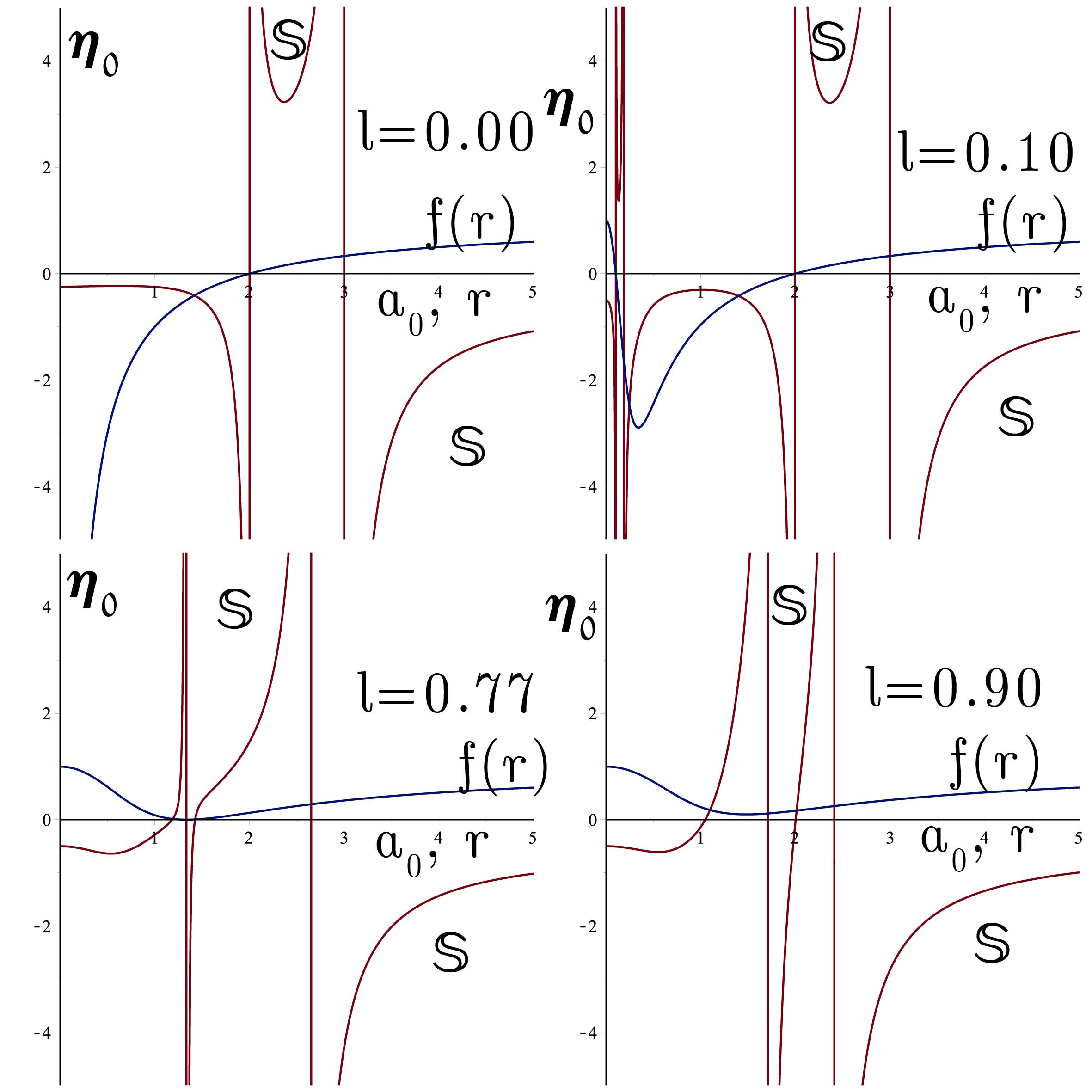
Figure 1: Stability of TSW supported by LG in terms of $a_{0}$ and $\eta_{0}$ for $\ell=0.00,0.10,0.77$ and $0.90.$ The value of $m=1.$ The effect of Hayward’s constant is to increase the stability of the TSW. We note that the stable regions are shown by $\mathcal{S}$ and the metric function is plotted too.

In the case of a linear EoS i.e.,

$$\psi=\eta_{0}\left(\sigma-\sigma_{0}\right)+p_{0}$$ (33)

in which $\eta_{0}$ is a constant parameter, one finds $\psi^{\prime}\left(\sigma_{0}\right)=\eta_{0}.$ Fig. 1 displays the region of stability in terms of $\eta_{0}$ and $a_{0}$ for different values of Hayward’s parameter.

IV.2 Chaplygin gas (CG)

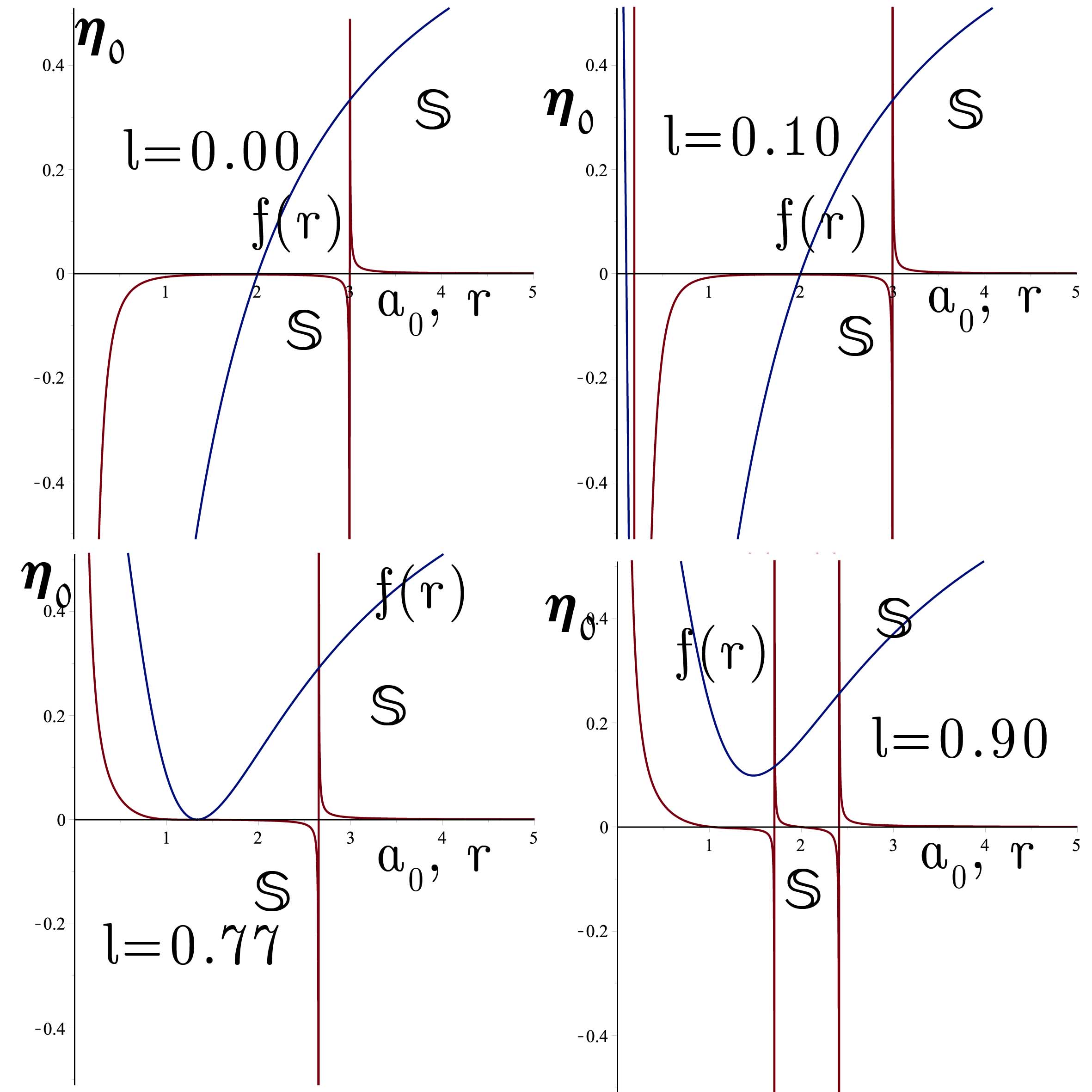
Figure 2: Stability of TSW supported by CG in terms of $a_{0}$ and $\eta_{0}$ for $\ell=0.00,0.10,0.77$ and $0.90.$ The value of $m=1.$ The effect of Hayward’s constant is to increase the stability of the TSW. We also plot the metric function to compare the horizon of the black hole and the location of the throat.

For Chaplygin gas (CG) the EoS is given by

$$\psi=\eta_{0}\left(\frac{1}{\sigma}-\frac{1}{\sigma_{0}}\right)+p_{0}$$ (34)

where $\eta_{0}$ is a constant parameter, implies $\psi^{\prime}\left(\sigma_{0}\right)=-\frac{\eta_{0}}{\sigma_{0}^{2}}.$ In Fig. 2 we plot the stability region in terms of $\eta_{0}$ and $a_{0}$ for different values of $\ell.$

IV.3 Generalized Chaplygin gas (GCG)

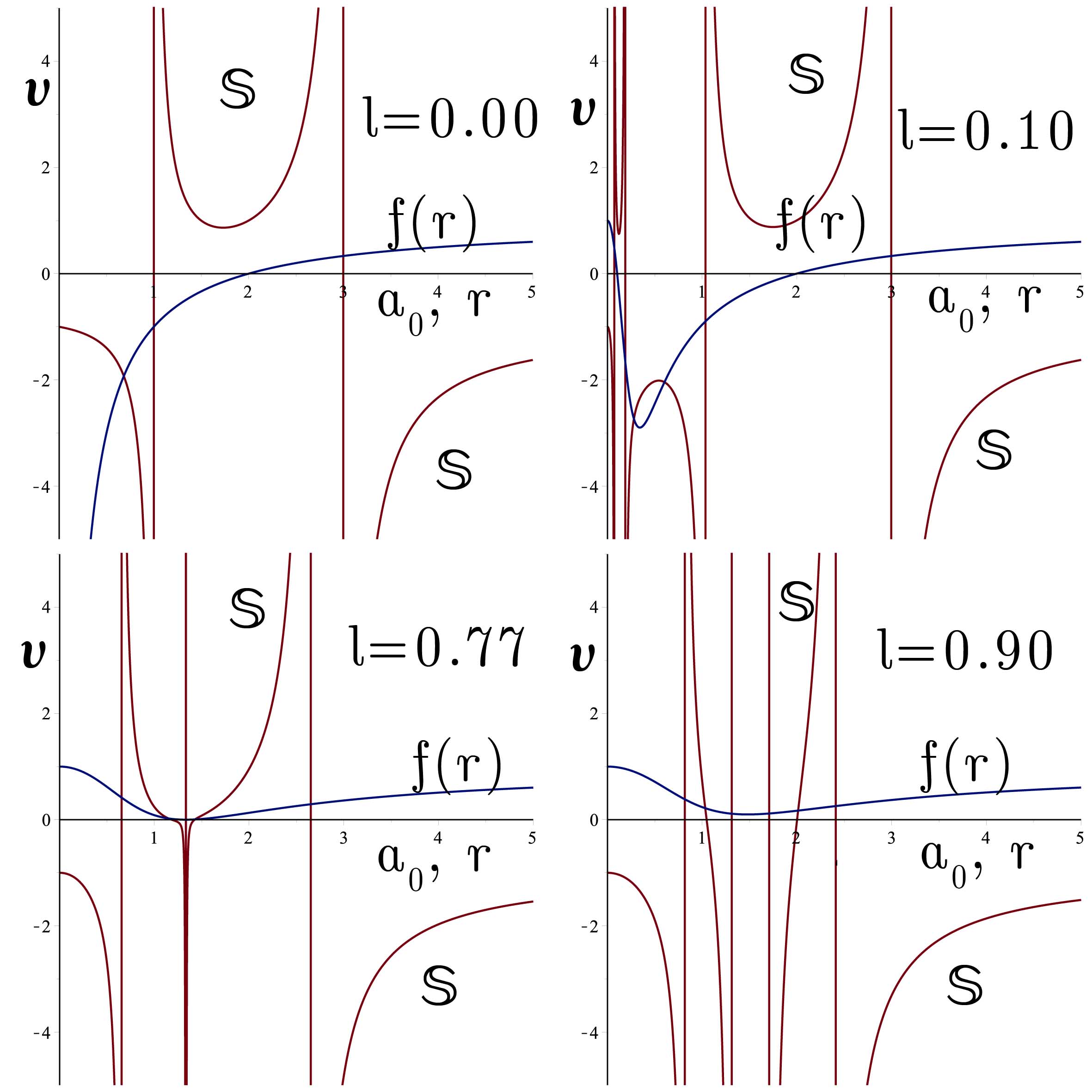
Figure 3: Stability of TSW supported by GCG in terms of $a_{0}$ and $\nu$ for $\ell=0.00,0.10,0.77$ and $0.90.$ The value of $m=1.$ The effect of Hayward’s constant is to increase the stability of the TSW. We also plot the metric function to compare the horizon of the black hole and the location of the throat.

The EoS of the Generalized Chaplygin gas can be cast into

$$\psi\left(\sigma\right)=\eta_{0}\left(\frac{1}{\sigma^{\nu}}-\frac{1}{\sigma_{0}^{\nu}}\right)+p_{0}$$ (35)

in which $\nu$ and $\eta_{0}$ are constants. To see the effect of parameter $\nu$ in the stability we set the constant $\eta_{0}$ such that $\psi$ becomes

$$\psi\left(\sigma\right)=p_{0}\left(\frac{\sigma_{0}}{\sigma}\right)^{\nu}.$$ (36)

We find $\psi^{\prime}\left(\sigma_{0}\right)=-\frac{p_{0}}{\sigma_{0}}\nu$ and in Fig. 3 we plot the stability regions of the TSW supported by a GCG in terms of $\nu$ and $a_{0}$ with various values of $\ell.$

IV.4 Modified Generalized Chaplygin gas (MGCG)

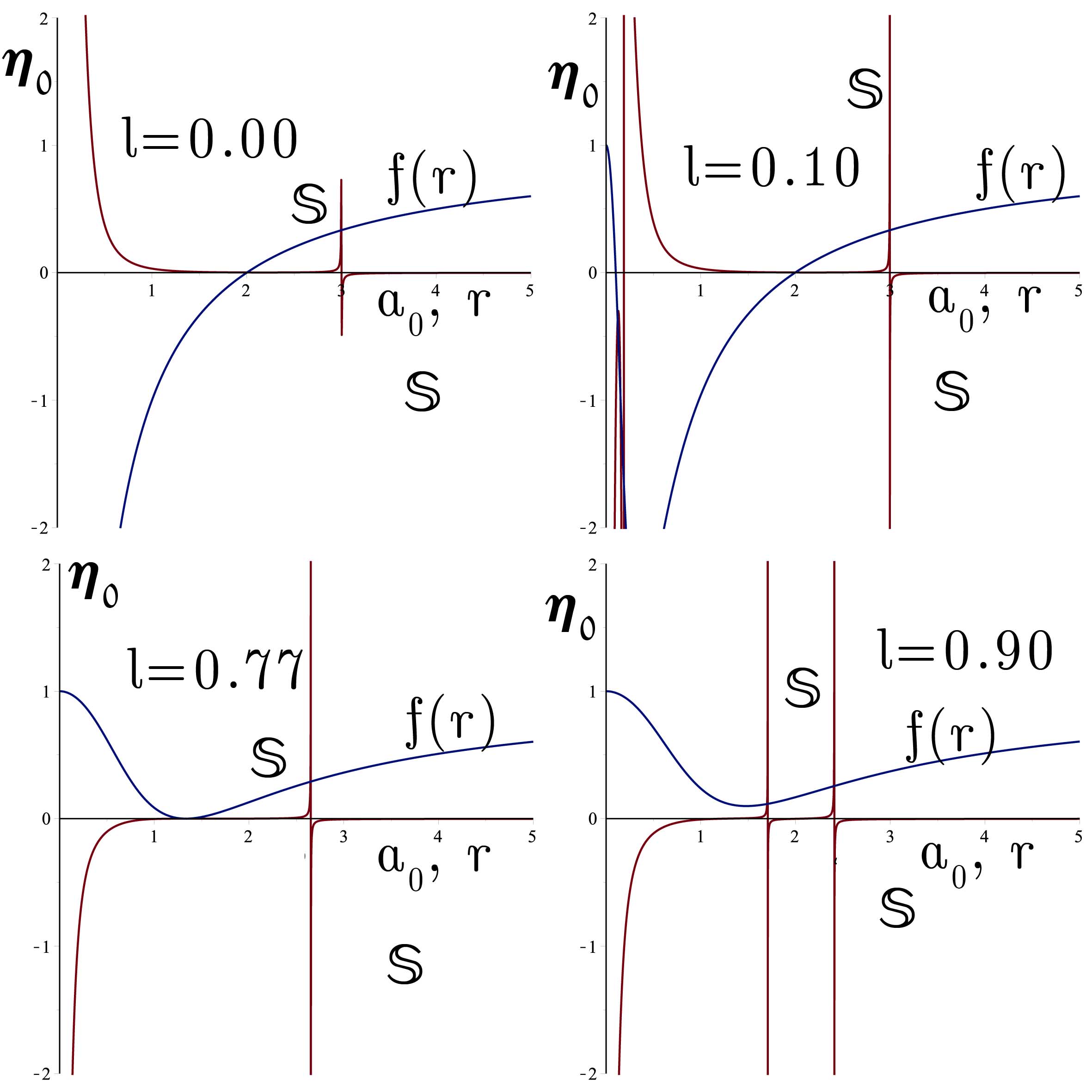
Figure 4: Stability of TSW supported by MGCG in terms of $a_{0}$ and $\eta_{0}$ for $\ell=0.00,0.10,0.77$ and $0.90.$ The value of $m=1$ and $\xi_{0}=\eta_{0}=1.$ The effect of Hayward’s constant is to increase the stability of the TSW. We also plot the metric function to compare the horizon of the black hole and the location of the throat.

A more general form of CG is called the Modified Generalized Chaplygin gas (MGCG) which is given by

$$\psi\left(\sigma\right)=\xi_{0}\left(\sigma-\sigma_{0}\right)-\eta_{0}\left(\frac{1}{\sigma^{\nu}}-\frac{1}{\sigma_{0}^{\nu}}\right)+p_{0}$$ (37)

in which $\xi_{0}$, $\eta_{0}$ and $\nu$ are free parameters. One then, finds

$$\psi^{\prime}\left(\sigma_{0}\right)=\xi_{0}+\eta_{0}\frac{\eta_{0}\nu}{\sigma_{0}^{\nu+1}}.$$ (38)

To go further we set $\xi_{0}=1$ and $\nu=1$ and in Fig. 4 we show the stability regions in terms of $\eta_{0}$ and $a_{0}$ with various values of $\ell$.

IV.5 Logarithmic gas (LogG)

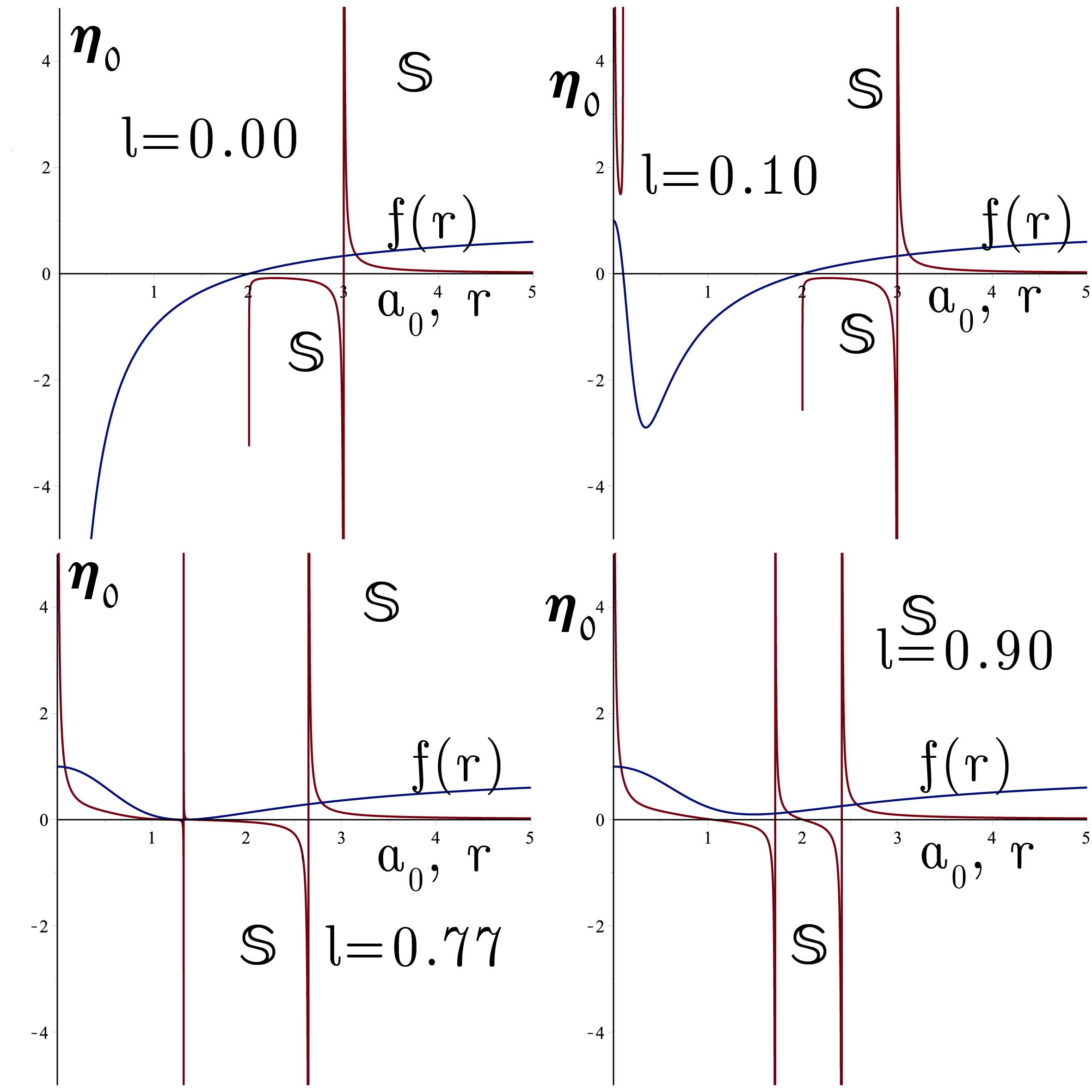
Figure 5: Stability of TSW supported by LogG in terms of $a_{0}$ and $\eta_{0}$ for $\ell=0.00,0.10,0.77$ and $0.90.$ The value of $m=1.$ The effect of Hayward’s constant is to increase the stability of the TSW. We also plot the metric function to compare the horizon of the black hole and the location of the throat.

In our last example we consider the Logarithmic gas (LogG) given by

$$\psi\left(\sigma\right)=\eta_{0}\ln\left|\frac{\sigma}{\sigma_{0}}\right|+p_{0}$$ (39)

in which $\eta_{0}$ is a constant. For LogG one finds

$$\psi^{\prime}\left(\sigma_{0}\right)=\frac{\eta_{0}}{\sigma_{0}}.$$ (40)

In Fig. 5 we plot the stability region for the TSW supported by LogG and the effect of Hayward’s parameter is shown clearly.

V Stability analysis for small velocity perturbations around the static solution

In this section we restrict ourselves to the small velocity perturbations about the equilibrium point $a=a_{0}$ such that at any proper time after the perturbation we can consider the fluid supporting the shell to be approximately static. Thus one can accept the dynamic EoS of the wormhole same as the static EoS 13 . This assumption, therefore, implies that the EoS is uniquely determined by $f\left(a\right)$ and $a$, described by Eqs. (22), (23) i.e.

$$p=-\frac{1}{2}\left(1+\frac{af^{\prime}\left(a\right)}{2f\left(a\right)}\right)\sigma.$$ (41)

With this EoS together with Eqs. (20) and (21) one finds the one-dimentional motion of the throat given by

$$\ddot{a}-\frac{f^{\prime}}{2f}\dot{a}^{2}=0.$$ (42)

Now, an integration from both sides implies

$$\dot{a}=\dot{a}_{0}\frac{\sqrt{f}}{\sqrt{f_{0}}}$$ (43)

and a second integration gives

$$\int_{a0}^{a}\frac{da}{\sqrt{f\left(a\right)}}=\frac{\dot{a}_{0}}{\sqrt{f_{0}}}\left(\tau-\tau_{0}\right).$$ (44)

Note that $\dot{a}_{0}$ for the equilibrium point is zero but here after perturbation we assume that the perturbation consists of an initial small velocity which we call it $\dot{a}_{0}.$

V.1 The Schwarzschild Example

The last integral (44) depends on the bulk metric, so that it gives different results for different spacetimes. For the Schwarzschild bulk, $f\left(a\right)=1-\frac{2m}{a}$ which a substitution in (44) yields

$$\frac{\dot{a}_{0}}{\sqrt{f_{0}}}\left(\tau-\tau_{0}\right)=a\sqrt{f}-a_{0}\sqrt{f_{0}}+m\ln\left(\frac{a-m+a\sqrt{f}}{a_{0}-m+a_{0}\sqrt{f_{0}}}\right).$$ (45)

This motion is not clearly oscillatory which indicates that the throat is unstable against the small velocity perturbation.

V.2 The Hayward Example

For the case of the Hayward bulk spacetime, Eq. (44), up to the second order of $\ell,$ admits

$$\frac{\dot{a}_{0}}{\sqrt{f_{0}}}\left(\tau-\tau_{0}\right)\tilde{=}a\sqrt{f}-\\ a_{0}\sqrt{f_{0}}+m\ln\left(\frac{a-m+a\sqrt{f}}{a_{0}-m+a_{0}\sqrt{f_{0}}}\right)+\\ 2\ell^{2}\left(\frac{2a^{2}-2am-m^{2}}{3ma^{2}\sqrt{f}}-\frac{2a_{0}^{2}-2a_{0}m-m^{2}}{3ma_{0}^{2}\sqrt{f_{0}}}\right).$$ (46)

Similar to the previous case, this motion is not also oscillatory which implies that the throat is unstable against the small velocity perturbation. Nevertheless, Eq. (42) shows that the acceleration of the throat is given by $\ddot{a}=\frac{f^{\prime}}{2f}\dot{a}^{2}$ which is positive for both the Schwarzschild and Hayward bulks. Thus the motion of the throat is not oscillatory and consequently the corresponding TSW is not stable.

VI Conclusion

Thin-shell wormholes are constructed from the regular black hole (or non-black hole for certain range of parameters) discovered by Hayward. We show first that this solution is powered by a magnetic monopole field within the context of non-linear electrodynamics (NED). The non-linear Lagrangian in the present case can be expressed in a non-polynomial form of the Maxwell invariant. Such a Lagrangian doesn’t admit a linear Maxwell limit. By employing the spacetime of Hayward and different equations of state of generic form $p=\psi\left(\sigma\right)$ on the thin-shell we plot possible stable regions. Amongst these linear, logarithmic and different Chaplygin gas forms are used and stable regions are displayed. The method of identifying these regions relies on the reduction of the perturbation equations to a harmonic equation of the form $\ddot{x}+\frac{1}{2}V^{\prime\prime}\left(a_{0}\right)x=0$ for $x=a-a_{0}.$ Stability simply amounts to the condition for $V^{\prime\prime}\left(a_{0}\right)>0$ which is plotted numerically. In all different equations of state we obtained stable regions and observed that the Hayward parameter $\ell$ plays a crucial role in establishing the stability. That is, for higher $\ell$ value we have enlargement in the stable region. The trivial case $\ell=0$ corresponds to the Schwarzschild case and is well-known. We have considered also perturbations with small velocity. It turns out that our TSW is no more stable against such kind of perturbations. We would like to add here that a stable spherically symmetric wormhole in general relativity has been introduced in 11 . Finally, we admit that in each case our energy density happens to be negative so that we are confronted with exotic matter. In a separate study we have shown that to have anything but exotic matter to thread the wormhole we have to abandon spherical symmetry and consider prolate / oblate spheroidal sources 12 .

References

- (1) M. Visser, Phys. Rev. D 39, 3182 (1989); M. Visser, Nucl. Phys. B 328, 203 (1989); P. R. Brady, J. Louko and E. Poisson, Phys. Rev. D 44, 1891 (1991); E. Poisson and M. Visser, Phys. Rev. D 52, 7318 (1995); M. Ishak and K. Lake, Phys. Rev. D 65, 044011 (2002); C. Simeone, Int. Jou. of Mod. Phys. D 21, 1250015 (2012); E. F. Eiroa and C. Simeone, Phys. Rev. D 82, 084039 (2010); F. S. Lobo, Phys. Rev. D 71, 124022 (2005); E. F. Eiroa and C. Simeone, Phys. Rev. D 71, 127501 (2005); E. F. Eiroa, Phys. Rev. D 78, 024018 (2008); F. S. N. Lobo and P. Crawford, Class. Quantum Grav. 22, 4869 (2005); N. M. Garcia, F. S. N. Lobo and M. Visser, Phys. Rev. D 86, 044026 (2012); S. H. Mazharimousavi, M. Halilsoy and Z. Amirabi, Phys. Lett. A 375, 3649 (2011); M. Sharif and M. Azam, Eur. Phys. J. C 73, 2407 (2013); M. Sharif and M. Azam, Eur. Phys. J. C 73, 2554 (2013); S. Habib Mazharimousavi and M. Halilsoy, Eur. Phys. J. C 73, 2527 (2013).
- (2) G. A. S. Dias and J. P. S. Lemos, Phys. Rev. D 82, 084023 (2010).
- (3) J. P. S. Lemos, F. S. N. Lobo, S. Q. Oliveira, Phys. Rev. D 68, 064004 (2003).
- (4) J. Bardeen, Proceedings of GR5, Tiflis, U.S.S.R. (1968); A. Borde , Phys.Rev. D 50, 3392(1994); A. Borde , Phys.Rev. D 55, 7615 (1997).
- (5) E. Ayon-Beato and A. Garcıa, Phys. Rev. Lett. 80, 5056 (1998).
- (6) K. Bronnikov, Phys. Rev. Lett. 85, 4641 (2000); K. Bronnikov, Phys. Rev. D 63, 044005 (2001); K. A. Bronnikov, V. N. Melnikov, G. N. Shikin and K. P. Staniukovich. Ann. Phys. (USA) 118, 84 (1979).
- (7) S. A. Hayward, Phys. Rev. Lett. 96, 031103 (2006).
- (8) W. Israel, Nuovo Cimento 44B, 1 (1966); V. de la Cruzand W. Israel, Nuovo Cimento 51A, 774 (1967); J. E. Chase, Nuovo Cimento 67B, 136. (1970); S. K. Blau, E. I. Guendelman, and A. H. Guth, Phys. Rev. D 35, 1747 (1987); R. Balbinot and E. Poisson, Phys. Rev. D 41, 395 (1990).
- (9) M. G. Richarte and C. Simeone, Phys. Rev. D 80, 104033 (2009); M. G. Richarte, Phys. Rev. D 82, 044021 (2010);
- (10) E. F. Eiroa and C. Simeone, Phys. Rev. D 76, 024021 (2007); F. S. N. Lobo, Phys. Rev. D 73, 064028 (2006);
- (11) V. Gorini, U. Moschella, A. Y. Kamenshchik, V. Pasquier and A. A. Starobinsky, Phys. Rev. D 78, 064064 (2008); V. Gorini, A. Y. Kamenshchik, U. Moschella,O. F. Piattella and A. A. Starobinsky, Phys. Rev. D 80, 104038(2009); E. F. Eiroa, Phys. Rev. D 80, 044033 (2009); C. Bejarano and E. F. Eiroa, Phys. Rev. D 84, 064043 (2011); E. F. Eiroa and G. F. Aguirre, Eur. Phys. J. C 72, 2240 (2012).
- (12) A. Y. Kamenshchik, U. Moschella and V. Pasquier, Phys. Lett. B 487, 7 (2000); L. P. Chimento, Phys. Rev. D 69, 123517 (2004); M. Sharif and M. Azam, JCAP 05, 25 (2013); M. Jamil, M. U. Farooq and M. A. Rashid, Eur. Phys. J. C 59, 907 (2009).
- (13) C. Bambi, L. Modesto, Phys. Lett. B 721, 329 (2013).
- (14) Z. Amirabi, M. Halilsoy and S. H. Mazharimousavi, Phys. Rev. D 88, 124023 (2013).
- (15) K. A. Bronnikov, L. N. Lipatova, I. D. Novikov and A. A. Shatskiy, Grav. Cosmol. 19, 269 (2013).
- (16) S. H. Mazharimousavi and M. Halilsoy, ”Thin-shell wormholes supported by normal matter”: arXiv:1311.6697.
- (17) M. G. Richarte, Phys. Rev. D 88, 027507 (2013); E. F. Eiroa and C. Simone, Phys. Rev. D 70, 044008 (2004); C. Bejarano, E. F. Eiroa, and C. Simeone, Phys. Rev. D 75, 027501 (2007); E. F. Eiroa and C. Simeone, Phys. Rev. D 81, 084022 (2010); M. G. Richarte and C. Simeone, Phys. Rev. D 79, 127502 (2009); E. Rubín de Celis, O. P. Santillán, and C. Simeone, Phys. Rev. D 86, 124009 (2012); M. Sharif and M. Azam, J. Cosmol. Astropart. Phys. 04, 023 (2013).