On the decay of the inverse of matrices
that are sum of Kronecker products

Claudio Canutoa, Valeria Simoncinib and Marco Veranic
Abstract

Decay patterns of matrix inverses have recently attracted considerable interest, due to their relevance in numerical analysis, and in applications requiring matrix function approximations. In this paper we analyze the decay pattern of the inverse of banded matrices in the form S=MβŠ—In+InβŠ—M𝑆tensor-product𝑀subscript𝐼𝑛tensor-productsubscript𝐼𝑛𝑀S=M\otimes I_{n}+I_{n}\otimes M where M𝑀M is tridiagonal, symmetric and positive definite, Insubscript𝐼𝑛I_{n} is the identity matrix, and βŠ—tensor-product\otimes stands for the Kronecker product. It is well known that the inverses of banded matrices exhibit an exponential decay pattern away from the main diagonal. However, the entries in Sβˆ’1superscript𝑆1S^{-1} show a non-monotonic decay, which is not caught by classical bounds. By using an alternative expression for Sβˆ’1superscript𝑆1S^{-1}, we derive computable upper bounds that closely capture the actual behavior of its entries. We also show that similar estimates can be obtained when M𝑀M has a larger bandwidth, or when the sum of Kronecker products involves two different matrices. Numerical experiments illustrating the new bounds are also reported.

aDipartimento di Scienze Matematiche, Politecnico di Torino, Corso Duca degli Abruzzi 24, I-10129 Torino, Italy
ccanuto@polito.it bDipartimento di Matematica, UniversitΓ  di Bologna, Piazza di Porta San Donato 5, I-40127 Bologna, Italy
valeria.simoncini@unibo.it cMOX - Dipartimento di Matematica, Politecnico di Milano, via Bonardi, 9, I-20133 Milano, Italy
marco.verani@polimi.it

1 Introduction

We consider nonsingular matrices S𝑆S of size n2Γ—n2superscript𝑛2superscript𝑛2n^{2}\times n^{2} that can be written as

S=MβŠ—In+InβŠ—M,𝑆tensor-product𝑀subscript𝐼𝑛tensor-productsubscript𝐼𝑛𝑀\displaystyle S=M\otimes I_{n}+I_{n}\otimes M, (1)

where M𝑀M is an nΓ—n𝑛𝑛n\times n banded symmetric and positive definite matrix (SPD) and βŠ—tensor-product\otimes is the Kronecker product; here Insubscript𝐼𝑛I_{n} is the identity matrix of size n𝑛n. Matrices in this form may arise for instance in the discretization of two-dimensional partial differential equations by means of finite difference, spectral or finite element methods. We say that a symmetric matrix A𝐴A is b𝑏b-banded if its entries Ai​jsubscript𝐴𝑖𝑗A_{ij} satisfy Ai​j=0subscript𝐴𝑖𝑗0A_{ij}=0 for |iβˆ’j|>b𝑖𝑗𝑏|i-j|>b. In the following, we shall mainly focus on the case when M𝑀M is tridiagonal, so that b=1𝑏1b=1. As a consequence of M𝑀M being banded, S𝑆S will also be banded, although its bandwidth will be much larger: if b𝑏b is the bandwidth of M𝑀M, then bβ‹…n⋅𝑏𝑛b\cdot n will be the bandwidth of S𝑆S.

We are interested in exploring the magnitude pattern of the entries (Sβˆ’1)i​jsubscriptsuperscript𝑆1𝑖𝑗(S^{-1})_{ij}. It is well-known that although the inverse of a banded matrix is full in general - and in particular it is not banded - its entries exponentially decay as their location deviates from the main diagonal; such a decay pattern was analyzed in detail in [12] for S𝑆S a general symmetric positive definite b𝑏b-banded matrix. Indeed, it was shown in [12] that

|(Sβˆ’1)i​j|≀γ​q|iβˆ’j|bsubscriptsuperscript𝑆1𝑖𝑗𝛾superscriptπ‘žπ‘–π‘—π‘\displaystyle|(S^{-1})_{ij}|\leq\gamma q^{\frac{|i-j|}{b}} (2)

where ΞΊπœ…\kappa is the condition number of S𝑆S, q=(ΞΊβˆ’1)/(ΞΊ+1)π‘žπœ…1πœ…1q=(\sqrt{\kappa}-1)/(\sqrt{\kappa}+1), Ξ³=max⁑{Ξ»min​(S)βˆ’1,Ξ³^}𝛾subscriptπœ†minsuperscript𝑆1^𝛾\gamma=\max\{\lambda_{\rm min}(S)^{-1},\hat{\gamma}\}, and Ξ³^=(1+ΞΊ)2/(2​λmax​(S))^𝛾superscript1πœ…22subscriptπœ†π‘†\hat{\gamma}=(1+\sqrt{\kappa})^{2}/(2\lambda_{\max}(S)); in this bound the diagonal elements of S𝑆S are assumed not to be greater than one. Here and in the following, Ξ»min​(β‹…),Ξ»max​(β‹…)subscriptπœ†β‹…subscriptπœ†β‹…\lambda_{\min}(\cdot),\lambda_{\max}(\cdot) denote the smallest and largest eigenvalues of the given symmetric matrix.

Decay patterns have attracted considerable interest in the scientific computing community in the last two decades, due to their relevance in the context of linear system preconditioning [6], [2], low-rank approximation strategies such as hierarchical matrices, wavelets etc. [23], [1], and in a large variety of applications requiring matrix function approximations, such as electronic structure calculations, complex networks, robotics, etc.; see, e.g., [4], [7],[5],[3],[17], and the references therein.

A large amount of literature has focused on the inverse entries of (irreducible) tridiagonal matrices for which explicit formulas and recurrence relations are now available; see, e.g., [21], [19] and their references. Some of these results can be generalized to block tridiagonal cases, of which (1) is a particular case for M𝑀M tridiagonal, however accurate estimates for the entries have only been obtained under more restrictive assumptions [20]. In [19], for instance, the case of the discretization of the two-dimensional Poisson operator was considered, which corresponds to (1) with M𝑀M SPD, tridiagonal and with constant coefficients (see Example 2.2 below).

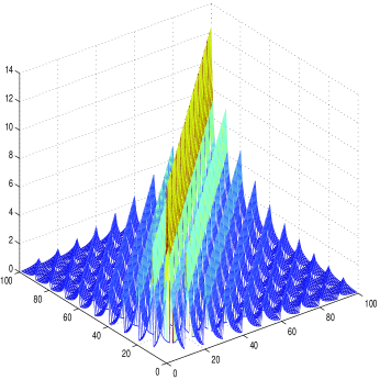
A key point of the matrices in the form (1) is that the decay of the entries of its inverse is not monotonic away from the diagonal. In fact, the entries decay in a way that recalls a sinusoidal behavior converging to zero. We report in Figure 1 a typical such pattern, obtained for M=βˆ’tridiag​(1,βˆ’2Β―,1)𝑀tridiag1Β―21M=-{\rm tridiag}(1,-\underline{2},1) (here and later in the paper, the underlined number lies on the matrix diagonal), corresponding to the finite difference discretization of the two-dimensional negative Laplace operator βˆ’(ux​x+uy​y)subscript𝑒π‘₯π‘₯subscript𝑒𝑦𝑦-(u_{xx}+u_{yy}) in the domain [0,1]Γ—[0,1]0101[0,1]\times[0,1]. This non-monotonic behavior has been observed in the literature ([19]), and explained in detail for the case of the discrete Laplacian, for which precise estimates are available [9], [18], [22]; bounds stemming from an algebraic analysis were also determined in [19]. The situation is far less understood when M𝑀M is any tridiagonal SPD matrix, or more generally any banded SPD matrix. Clearly, classical bounds such as the one in (2) cannot catch this non-monotonic pattern, although its detection can be crucial in sparsity-based approximation procedures. In this paper we derive bounds that closely capture this non-monotonic behavior, which is typical of matrices in the form (1).
Refer to caption
Figure 1: Pattern of the inverse of the 2D Laplace 100Γ—100100100100\times 100 matrix in the unit square.

In particular, we show that the decaying oscillation observed in practice in |(Sβˆ’1)i,j|subscriptsuperscript𝑆1𝑖𝑗|(S^{-1})_{i,j}| for i,j=1,…,n2formulae-sequence𝑖𝑗1…superscript𝑛2i,j=1,\ldots,n^{2}, strongly depends on, and can be bounded by, the β€œmesh” distance between the two indices i,j𝑖𝑗i,j when each of them is represented in a natural nΓ—n𝑛𝑛n\times n grid. In section 2 we provide sharp estimates, followed by easily computable more qualitative bounds; the latter can be incorporated, for instance, in numerical thresholding strategies during a sparsity-oriented approximation of the matrix inverse (see, e.g., section 3).

In section 4 we shall extend our results to banded SPD matrices, and to the more general case

Sg:=M1βŠ—In+InβŠ—M2,assignsubscript𝑆𝑔tensor-productsubscript𝑀1subscript𝐼𝑛tensor-productsubscript𝐼𝑛subscript𝑀2\displaystyle S_{g}:=M_{1}\otimes I_{n}+I_{n}\otimes M_{2}, (3)

where M1subscript𝑀1M_{1} and M2subscript𝑀2M_{2} are symmetric tridiagonal matrices stemming, for instance, from the discretization by finite differences of a self-adjoint separable second order differential operator on a stretched rectangular domain, or of an operator with different coefficients in the two space directions; see, e.g., [16].

2 Decay of the entries of the inverse of S𝑆S for M𝑀M tridiagonal

Let X=Sβˆ’1𝑋superscript𝑆1X=S^{-1}, and write X=[x1,…,xt,…,xn2]𝑋subscriptπ‘₯1…subscriptπ‘₯𝑑…subscriptπ‘₯superscript𝑛2X=[x_{1},\ldots,x_{t},\ldots,x_{n^{2}}]. A simple but key observation is that each column t𝑑t of the inverse X𝑋X is the solution to the linear system

S​xt=et,𝑆subscriptπ‘₯𝑑subscript𝑒𝑑Sx_{t}=e_{t},

where etsubscript𝑒𝑑e_{t} is the t𝑑t-th column of In2subscript𝐼superscript𝑛2I_{n^{2}}. Let us define 𝒲tsubscript𝒲𝑑{\cal W}_{t} to be the matrix such that wt=vec​(𝒲t)subscript𝑀𝑑vecsubscript𝒲𝑑w_{t}={\rm vec}({\cal W}_{t}) with wtβˆˆβ„n2subscript𝑀𝑑superscriptℝsuperscript𝑛2w_{t}\in{\mathbb{R}}^{n^{2}} and 𝒲tβˆˆβ„nΓ—nsubscript𝒲𝑑superscriptℝ𝑛𝑛{\cal W}_{t}\in{\mathbb{R}}^{n\times n} (the β€œvec” operation stacks the columns of 𝒲tsubscript𝒲𝑑{\cal W}_{t} one below the other). With this notation, and using the Kronecker form of S𝑆S, the system above is equivalent to

M​𝒳t+𝒳t​M=β„°t.𝑀subscript𝒳𝑑subscript𝒳𝑑𝑀subscriptℰ𝑑M{\cal X}_{t}+{\cal X}_{t}M={\cal E}_{t}.

Since et=vec​(β„°t)subscript𝑒𝑑vecsubscriptℰ𝑑e_{t}={\rm vec}({\cal E}_{t}), t=1,…,n2𝑑1…superscript𝑛2t=1,\ldots,n^{2}, the matrix β„°tsubscriptℰ𝑑{\cal E}_{t} has a single nonzero element (β„°t)i​jsubscriptsubscriptℰ𝑑𝑖𝑗({\cal E}_{t})_{ij}, with indices j=⌊(tβˆ’1)/nβŒ‹+1𝑗𝑑1𝑛1j=\lfloor(t-1)/n\rfloor+1, i=tβˆ’nβ€‹βŒŠ(tβˆ’1)/nβŒ‹π‘–π‘‘π‘›π‘‘1𝑛i=t-n\lfloor(t-1)/n\rfloor, i,j∈{1,…,n}𝑖𝑗1…𝑛i,j\in\{1,\ldots,n\}. Therefore, we can write β„°t=β„°i+n​(jβˆ’1)=ei​ej⊀subscriptℰ𝑑subscriptℰ𝑖𝑛𝑗1subscript𝑒𝑖superscriptsubscript𝑒𝑗top{\cal E}_{t}={\cal E}_{i+n(j-1)}=e_{i}e_{j}^{\top}.

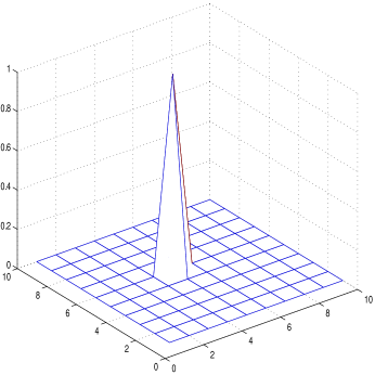
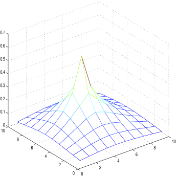
The derivation above shows that the n2superscript𝑛2n^{2} entries of each column of Sβˆ’1superscript𝑆1S^{-1}, properly reordered, correspond to the nΓ—n𝑛𝑛n\times n entries of the solution matrix to a Lyapunov equation. In Figure 2 we report the pattern of β„°tsubscriptℰ𝑑{\cal E}_{t} (left) and of 𝒳tsubscript𝒳𝑑{\cal X}_{t} (right) for t=26𝑑26t=26 when S𝑆S is the finite difference discretization of the two-dimensional Laplace operator in the unit square. Note that because of the isotropy property of the operator, the forcing term (the right-hand side) diffuses in a similar way in both directions; see also a related discussion in [19, section 4.1].

We next exploit the closed form of the Lyapunov solution to derive bounds for the entries of S:,tβˆ’1=vec​(𝒳t)subscriptsuperscript𝑆1:𝑑vecsubscript𝒳𝑑S^{-1}_{:,t}={\rm vec}({\cal X}_{t}) for each t=1,…,n2𝑑1…superscript𝑛2t=1,\ldots,n^{2}. Let j=⌊(tβˆ’1)/nβŒ‹+1𝑗𝑑1𝑛1j=\lfloor(t-1)/n\rfloor+1, i=tβˆ’nβ€‹βŒŠ(tβˆ’1)/nβŒ‹π‘–π‘‘π‘›π‘‘1𝑛i=t-n\lfloor(t-1)/n\rfloor. Since M𝑀M is positive definite, the solution can be written as (see, e.g., [15])

𝒳tsubscript𝒳𝑑\displaystyle{\cal X}_{t} =\displaystyle= 12β€‹Ο€β€‹βˆ«βˆ’βˆžβˆž(ı​ω​I+M)βˆ’1​ℰt​(ı​ω​I+M)βˆ’βˆ—β€‹dΟ‰12πœ‹superscriptsubscriptsuperscriptitalic-Δ±πœ”πΌπ‘€1subscriptℰ𝑑superscriptitalic-Δ±πœ”πΌπ‘€absentdifferential-dπœ”\displaystyle\frac{1}{2\pi}\int_{-\infty}^{\infty}(\imath\omega I+M)^{-1}{\cal E}_{t}(\imath\omega I+M)^{-*}{\rm d}\omega
=\displaystyle= 12β€‹Ο€β€‹βˆ«βˆ’βˆžβˆž(ı​ω​I+M)βˆ’1​ei​ejβŠ€β€‹(ı​ω​I+M)βˆ’βˆ—β€‹dω≑12β€‹Ο€β€‹βˆ«βˆ’βˆžβˆžzi​zjβˆ—β€‹dΟ‰12πœ‹superscriptsubscriptsuperscriptitalic-Δ±πœ”πΌπ‘€1subscript𝑒𝑖superscriptsubscript𝑒𝑗topsuperscriptitalic-Δ±πœ”πΌπ‘€absentdifferential-dπœ”12πœ‹superscriptsubscriptsubscript𝑧𝑖superscriptsubscript𝑧𝑗differential-dπœ”\displaystyle\frac{1}{2\pi}\int_{-\infty}^{\infty}(\imath\omega I+M)^{-1}e_{i}e_{j}^{\top}(\imath\omega I+M)^{-*}{\rm d}\omega\equiv\frac{1}{2\pi}\int_{-\infty}^{\infty}z_{i}z_{j}^{*}{\rm d}\omega

where zi=(ı​ω​I+M)βˆ’1​eisubscript𝑧𝑖superscriptitalic-Δ±πœ”πΌπ‘€1subscript𝑒𝑖z_{i}=(\imath\omega I+M)^{-1}e_{i}. We are interested in estimating the kπ‘˜k-th entry of the t𝑑t-th column of the inverse Sβˆ’1superscript𝑆1S^{-1}. Using

Refer to caption
Refer to caption
Figure 2: Left: Column 46 of the 100Γ—100100100100\times 100 identity matrix, represented on a 10Γ—10101010\times 10 grid. Right: Column 46 of the inverse Laplacian, represented on a 10Γ—10101010\times 10 grid.
m=⌊(kβˆ’1)/nβŒ‹+1,β„“=kβˆ’nβ€‹βŒŠ(kβˆ’1)/nβŒ‹,formulae-sequenceπ‘šπ‘˜1𝑛1β„“π‘˜π‘›π‘˜1𝑛\displaystyle m=\lfloor(k-1)/n\rfloor+1,\quad\ell=k-n\lfloor(k-1)/n\rfloor, (4)

this corresponds to estimating the entry (𝒳t)β„“,m=eβ„“βŠ€β€‹π’³t​emsubscriptsubscriptπ’³π‘‘β„“π‘šsuperscriptsubscript𝑒ℓtopsubscript𝒳𝑑subscriptπ‘’π‘š({\cal X}_{t})_{\ell,m}=e_{\ell}^{\top}{\cal X}_{t}e_{m} of 𝒳tsubscript𝒳𝑑{\cal X}_{t}, that is

(Sβˆ’1)k,t=(Sβˆ’1)β„“+n​(mβˆ’1),t=eβ„“βŠ€β€‹π’³t​em,β„“,m∈{1,…,n}.formulae-sequencesubscriptsuperscript𝑆1π‘˜π‘‘subscriptsuperscript𝑆1β„“π‘›π‘š1𝑑superscriptsubscript𝑒ℓtopsubscript𝒳𝑑subscriptπ‘’π‘šβ„“π‘š1…𝑛(S^{-1})_{k,t}=(S^{-1})_{\ell+n(m-1),t}=e_{\ell}^{\top}{\cal X}_{t}e_{m},\quad\ell,m\in\{1,\ldots,n\}.

By varying m,β„“βˆˆ{1,…,n}π‘šβ„“1…𝑛m,\ell\in\{1,\ldots,n\} all the elements of the t𝑑t-th column, (Sβˆ’1):,tsubscriptsuperscript𝑆1:𝑑(S^{-1})_{:,t} are obtained. We have

eβ„“βŠ€β€‹π’³t​em=12β€‹Ο€β€‹βˆ«βˆ’βˆžβˆžeβ„“βŠ€β€‹zi​(Ο‰)​zj​(Ο‰)βˆ—β€‹em​dΟ‰,superscriptsubscript𝑒ℓtopsubscript𝒳𝑑subscriptπ‘’π‘š12πœ‹superscriptsubscriptsuperscriptsubscript𝑒ℓtopsubscriptπ‘§π‘–πœ”subscript𝑧𝑗superscriptπœ”subscriptπ‘’π‘šdifferential-dπœ”e_{\ell}^{\top}{\cal X}_{t}e_{m}=\frac{1}{2\pi}\int_{-\infty}^{\infty}e_{\ell}^{\top}z_{i}(\omega)z_{j}(\omega)^{*}e_{m}{\rm d}\omega,

so that

|eβ„“βŠ€β€‹π’³t​em|≀12β€‹Ο€β€‹βˆ«βˆ’βˆžβˆž|eβ„“βŠ€β€‹zi​(Ο‰)|​|zj​(Ο‰)βˆ—β€‹em|​dΟ‰.superscriptsubscript𝑒ℓtopsubscript𝒳𝑑subscriptπ‘’π‘š12πœ‹superscriptsubscriptsuperscriptsubscript𝑒ℓtopsubscriptπ‘§π‘–πœ”subscript𝑧𝑗superscriptπœ”subscriptπ‘’π‘šdifferential-dπœ”\displaystyle|e_{\ell}^{\top}{\cal X}_{t}e_{m}|\leq\frac{1}{2\pi}\int_{-\infty}^{\infty}|e_{\ell}^{\top}z_{i}(\omega)|\,|z_{j}(\omega)^{*}e_{m}|\,{\rm d}\omega. (5)

Since eβ„“βŠ€β€‹zi​(Ο‰)=eβ„“βŠ€β€‹(ı​ω​I+M)βˆ’1​eisuperscriptsubscript𝑒ℓtopsubscriptπ‘§π‘–πœ”superscriptsubscript𝑒ℓtopsuperscriptitalic-Δ±πœ”πΌπ‘€1subscript𝑒𝑖e_{\ell}^{\top}z_{i}(\omega)=e_{\ell}^{\top}(\imath\omega I+M)^{-1}e_{i}, the first term in the integrand above is the absolute value of the (β„“,i)ℓ𝑖(\ell,i) entry of the inverse of tridiagonal matrix (ı​ω​I+M)italic-Δ±πœ”πΌπ‘€(\imath\omega I+M). In the following we shall bound each of the two integrand terms, and then we will estimate the obtained integral.

Let Ξ»min,Ξ»maxsubscriptπœ†subscriptπœ†\lambda_{\min},\lambda_{\max} be the extreme eigenvalues of M𝑀M, and let Ξ»1=Ξ»min+ı​ωsubscriptπœ†1subscriptπœ†italic-Δ±πœ”\lambda_{1}=\lambda_{\min}+\imath\omega, Ξ»2=Ξ»max+ı​ωsubscriptπœ†2subscriptπœ†italic-Δ±πœ”\lambda_{2}=\lambda_{\max}+\imath\omega. The matrix ı​ω​I+Mitalic-Δ±πœ”πΌπ‘€\imath\omega I+M is a purely imaginary shifted version of the tridiagonal matrix M𝑀M, and its inverse shows a decreasing pattern, in spite of the complex shift. While estimates for |eβ„“βŠ€β€‹(ı​ω​I+M)βˆ’1​ei|superscriptsubscript𝑒ℓtopsuperscriptitalic-Δ±πœ”πΌπ‘€1subscript𝑒𝑖|e_{\ell}^{\top}(\imath\omega I+M)^{-1}e_{i}| are well known for Ο‰=0πœ”0\omega=0 (see, e.g., [12, 20, 19]), upper bounds for Ο‰β‰ 0πœ”0\omega\neq 0 are less so. Upper bounds for |eβ„“βŠ€β€‹(ı​ω​I+M)βˆ’1​ei|superscriptsubscript𝑒ℓtopsuperscriptitalic-Δ±πœ”πΌπ‘€1subscript𝑒𝑖|e_{\ell}^{\top}(\imath\omega I+M)^{-1}e_{i}|, Ο‰β‰ 0πœ”0\omega\neq 0 were given by Freund in [13, Theorem 6], and we recall this result for future reference.

Proposition 2.1.

Assume M𝑀M is symmetric positive definite and b𝑏b-banded. Let a=(Ξ»1+Ξ»2)/(Ξ»2βˆ’Ξ»1)π‘Žsubscriptπœ†1subscriptπœ†2subscriptπœ†2subscriptπœ†1a=(\lambda_{1}+\lambda_{2})/(\lambda_{2}-\lambda_{1}), and R>1𝑅1R>1 be defined as R=Ξ±+Ξ±2βˆ’1𝑅𝛼superscript𝛼21R=\alpha+\sqrt{\alpha^{2}-1}, with Ξ±=(|Ξ»1|+|Ξ»2|)/|Ξ»2βˆ’Ξ»1|𝛼subscriptπœ†1subscriptπœ†2subscriptπœ†2subscriptπœ†1\alpha=(|\lambda_{1}|+|\lambda_{2}|)/|\lambda_{2}-\lambda_{1}|. Then

|eβ„“βŠ€β€‹(ı​ω​I+M)βˆ’1​ei|≀2​R|Ξ»1βˆ’Ξ»2|​B​(a)​(1R)|β„“βˆ’i|b,β„“β‰ i,formulae-sequencesuperscriptsubscript𝑒ℓtopsuperscriptitalic-Δ±πœ”πΌπ‘€1subscript𝑒𝑖2𝑅subscriptπœ†1subscriptπœ†2π΅π‘Žsuperscript1𝑅ℓ𝑖𝑏ℓ𝑖|e_{\ell}^{\top}(\imath\omega I+M)^{-1}e_{i}|\leq\frac{2R}{|\lambda_{1}-\lambda_{2}|}B(a)\left(\frac{1}{R}\right)^{\frac{|\ell-i|}{b}},\quad\ell\neq i,

where, writing a=Ξ±R​cos⁑(ψ)+ı​βR​sin⁑(ψ)π‘Žsubscriptπ›Όπ‘…πœ“italic-Δ±subscriptπ›½π‘…πœ“a=\alpha_{R}\cos(\psi)+\imath\beta_{R}\sin(\psi),

B​(a):=RΞ²R​αR2βˆ’cos2⁑(ψ)​(Ξ±R+Ξ±R2βˆ’cos2⁑(ψ)),assignπ΅π‘Žπ‘…subscript𝛽𝑅superscriptsubscript𝛼𝑅2superscript2πœ“subscript𝛼𝑅superscriptsubscript𝛼𝑅2superscript2πœ“B(a):=\frac{R}{\beta_{R}\sqrt{\alpha_{R}^{2}-\cos^{2}(\psi)}(\alpha_{R}+\sqrt{\alpha_{R}^{2}-\cos^{2}(\psi)})},

with Ξ±R=12​(R+1R)subscript𝛼𝑅12𝑅1𝑅\alpha_{R}=\frac{1}{2}(R+\frac{1}{R}) and Ξ²R=12​(Rβˆ’1R)subscript𝛽𝑅12𝑅1𝑅\beta_{R}=\frac{1}{2}(R-\frac{1}{R}).

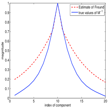
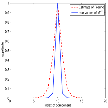
Clearly, R=R​(Ο‰)π‘…π‘…πœ”R=R(\omega). We omit this explicit dependence in the following. Figure 3 reports two typical behaviors of the bound in Proposition 2.1, for the pentadiagonal matrix in Example 4.1. The plots refer to Ο‰=0.10πœ”0.10\omega=0.10 (left) and Ο‰=10πœ”10\omega=10 (right): while the bound accurately captures the slope for large Ο‰πœ”\omega, this is in general less so for small Ο‰πœ”\omega. This difference in accuracy in general may affect the accuracy of our estimates, especially when a bandwidth b𝑏b greater than one is used (here b=2𝑏2b=2).

Refer to caption
Refer to caption
Figure 3: Typical estimate of Proposition 2.1 (column 10) for the inverse of the pentadiagonal matrix of Example 4.1. Left: Ο‰=0.1πœ”0.1\omega=0.1. Right: Ο‰=10πœ”10\omega=10.

Since in this section we assume that M𝑀M is tridiagonal, we shall use the result above for b=1𝑏1b=1; the case b>1𝑏1b>1 is explored in section 4. We prove our bound in two steps. In the first step (Proposition 2.2), we estimate the entries in terms of an integral, which can be easily estimated numerically; the results appear to be quite accurate in our examples. In the second step (Proposition 2.3), we complete the upper bound by estimating the integrals, thus incurring in additional inaccuracies. The final bound (Propositions 2.3-2.4) should be considered as a qualitative estimate for the entries pattern.

Proposition 2.2.

For k,t∈{1,…,n2}π‘˜π‘‘1…superscript𝑛2k,t\in\{1,\ldots,n^{2}\}, let

j=⌊(tβˆ’1)/nβŒ‹+1,i=tβˆ’nβ€‹βŒŠ(tβˆ’1)/nβŒ‹,formulae-sequence𝑗𝑑1𝑛1𝑖𝑑𝑛𝑑1𝑛j=\lfloor(t-1)/n\rfloor+1,\quad i=t-n\lfloor(t-1)/n\rfloor,

and β„“,mβ„“π‘š\ell,m as in (4). With the notation above, the following holds.

i) If i≠ℓ𝑖ℓi\neq\ell and jβ‰ mπ‘—π‘šj\neq m, then

|(Sβˆ’1)k,t|≀12​π​64|Ξ»maxβˆ’Ξ»min|2β€‹βˆ«βˆ’βˆžβˆž(R2(R2βˆ’1)2)2​(1R)|iβˆ’β„“|+|jβˆ’m|βˆ’2​dΟ‰;subscriptsuperscript𝑆1π‘˜π‘‘12πœ‹64superscriptsubscriptπœ†subscriptπœ†2superscriptsubscriptsuperscriptsuperscript𝑅2superscriptsuperscript𝑅2122superscript1π‘…π‘–β„“π‘—π‘š2differential-dπœ”|(S^{-1})_{k,t}|\leq\frac{1}{2\pi}\frac{64}{|\lambda_{\max}-\lambda_{\min}|^{2}}\int_{-\infty}^{\infty}\left(\frac{R^{2}}{(R^{2}-1)^{2}}\right)^{2}\left(\frac{1}{R}\right)^{|i-\ell|+|j-m|-2}{\rm d}\omega;

ii) If either i=ℓ𝑖ℓi=\ell or j=mπ‘—π‘šj=m, then

|(Sβˆ’1)k,t|≀12​π​8|Ξ»maxβˆ’Ξ»min|β€‹βˆ«βˆ’βˆžβˆž1Ξ»min2+Ο‰2​R2(R2βˆ’1)2​(1R)|iβˆ’β„“|+|jβˆ’m|βˆ’1​dΟ‰;subscriptsuperscript𝑆1π‘˜π‘‘12πœ‹8subscriptπœ†subscriptπœ†superscriptsubscript1superscriptsubscriptπœ†2superscriptπœ”2superscript𝑅2superscriptsuperscript𝑅212superscript1π‘…π‘–β„“π‘—π‘š1differential-dπœ”|(S^{-1})_{k,t}|\leq\frac{1}{2\pi}\frac{8}{|\lambda_{\max}-\lambda_{\min}|}\int_{-\infty}^{\infty}\frac{1}{\sqrt{\lambda_{\min}^{2}+\omega^{2}}}\frac{R^{2}}{(R^{2}-1)^{2}}\left(\frac{1}{R}\right)^{|i-\ell|+|j-m|-1}{\rm d}\omega;

iii) If both i=ℓ𝑖ℓi=\ell and j=mπ‘—π‘šj=m, then

|(Sβˆ’1)k,t|≀12β€‹Ο€β€‹βˆ«βˆ’βˆžβˆž1Ξ»min2+Ο‰2​dΟ‰=12​λmin.subscriptsuperscript𝑆1π‘˜π‘‘12πœ‹superscriptsubscript1superscriptsubscriptπœ†2superscriptπœ”2differential-dπœ”12subscriptπœ†|(S^{-1})_{k,t}|\leq\frac{1}{2\pi}\int_{-\infty}^{\infty}\frac{1}{\lambda_{\min}^{2}+\omega^{2}}{\rm d}\omega=\frac{1}{2\lambda_{\min}}.
Proof.

To prove i), we recall that |(Sβˆ’1)k,t|=|eβ„“βŠ€β€‹π’³t​em|subscriptsuperscript𝑆1π‘˜π‘‘superscriptsubscript𝑒ℓtopsubscript𝒳𝑑subscriptπ‘’π‘š|(S^{-1})_{k,t}|=|e_{\ell}^{\top}{\cal X}_{t}e_{m}| so that (5) holds, and we notice that Ξ±R2βˆ’1=Ξ²R2superscriptsubscript𝛼𝑅21superscriptsubscript𝛽𝑅2\alpha_{R}^{2}-1=\beta_{R}^{2} and Ξ±R+Ξ²R=Rsubscript𝛼𝑅subscript𝛽𝑅𝑅\alpha_{R}+\beta_{R}=R. Moreover, 1Ξ±R2βˆ’cos2⁑(ψ)≀1/(Ξ±R2βˆ’1)1superscriptsubscript𝛼𝑅2superscript2πœ“1superscriptsubscript𝛼𝑅21\frac{1}{\sqrt{\alpha_{R}^{2}-\cos^{2}(\psi)}}\leq 1/(\sqrt{\alpha_{R}^{2}-1}). Therefore,

B​(a)≀RΞ²R​αR2βˆ’1​(Ξ±R+Ξ±R2βˆ’1)=RΞ²R2​(Ξ±R+Ξ²R)=1Ξ²R2,π΅π‘Žπ‘…subscript𝛽𝑅superscriptsubscript𝛼𝑅21subscript𝛼𝑅superscriptsubscript𝛼𝑅21𝑅superscriptsubscript𝛽𝑅2subscript𝛼𝑅subscript𝛽𝑅1superscriptsubscript𝛽𝑅2\displaystyle B(a)\leq\frac{R}{\beta_{R}\sqrt{\alpha_{R}^{2}-1}(\alpha_{R}+\sqrt{\alpha_{R}^{2}-1})}=\frac{R}{\beta_{R}^{2}(\alpha_{R}+\beta_{R})}=\frac{1}{\beta_{R}^{2}},

so that, using Proposition 2.1,

|eβ„“βŠ€β€‹(ı​ω​I+M)βˆ’1​ei|≀2​R|Ξ»1βˆ’Ξ»2|​4​R2(R2βˆ’1)2​(1R)|β„“βˆ’i|.superscriptsubscript𝑒ℓtopsuperscriptitalic-Δ±πœ”πΌπ‘€1subscript𝑒𝑖2𝑅subscriptπœ†1subscriptπœ†24superscript𝑅2superscriptsuperscript𝑅212superscript1𝑅ℓ𝑖|e_{\ell}^{\top}(\imath\omega I+M)^{-1}e_{i}|\leq\frac{2R}{|\lambda_{1}-\lambda_{2}|}\frac{4R^{2}}{(R^{2}-1)^{2}}\left(\frac{1}{R}\right)^{|\ell-i|}.

Substituting the estimate for each of the two integrand terms in (5), we obtain

|eβ„“βŠ€β€‹π’³t​em|≀12​π​64|Ξ»1βˆ’Ξ»2|2β€‹βˆ«βˆ’βˆžβˆžR2​R2(R2βˆ’1)2​R2(R2βˆ’1)2​(1R)|β„“βˆ’i|​(1R)|mβˆ’j|​dΟ‰,superscriptsubscript𝑒ℓtopsubscript𝒳𝑑subscriptπ‘’π‘š12πœ‹64superscriptsubscriptπœ†1subscriptπœ†22superscriptsubscriptsuperscript𝑅2superscript𝑅2superscriptsuperscript𝑅212superscript𝑅2superscriptsuperscript𝑅212superscript1𝑅ℓ𝑖superscript1π‘…π‘šπ‘—differential-dπœ”|e_{\ell}^{\top}{\cal X}_{t}e_{m}|\leq\frac{1}{2\pi}\frac{64}{|\lambda_{1}-\lambda_{2}|^{2}}\int_{-\infty}^{\infty}R^{2}\frac{R^{2}}{(R^{2}-1)^{2}}\frac{R^{2}}{(R^{2}-1)^{2}}\left(\frac{1}{R}\right)^{|\ell-i|}\left(\frac{1}{R}\right)^{|m-j|}{\rm d}\omega,

from which the result follows.

As of ii) we only need to notice that if, for instance, β„“=iℓ𝑖\ell=i, then

|eβ„“βŠ€β€‹(ı​ω​I+M)βˆ’1​ei|≀1|Ξ»min+ı​ω|.superscriptsubscript𝑒ℓtopsuperscriptitalic-Δ±πœ”πΌπ‘€1subscript𝑒𝑖1subscriptπœ†italic-Δ±πœ”\displaystyle|e_{\ell}^{\top}(\imath\omega I+M)^{-1}e_{i}|\leq\frac{1}{|\lambda_{\min}+\imath\omega|}. (6)

Substituting into the integral, the bound follows as in the previous case.

For the case iii), the bound (6) can be used for both pairs of indices, and the final bound follows. ∎

We next report on a few examples showing the quality of the estimates in PropositionΒ 2.2. As one might expect, the factor in front of the integral slightly deteriorates the estimate, while qualitatively the decay of the entries in the inverse matrix is perfectly captured. We observe that the bounds ii) and iii) can be very loose because of the estimate’s weakness in (6). This can be clearly observed in the numerical experiments, below, where the inaccuracy of our estimate is more pronounced in correspondence with the highest peaks, namely for β„“=iℓ𝑖\ell=i and/or m=jπ‘šπ‘—m=j. In all examples, the matrix M𝑀M was scaled by its diagonal, so as to have entries all not greater than one. Technically, the integral appearing in the bound was estimated using the adaptive Gauss-Kronrod quadrature rule (Matlab function quadgk).
Refer to caption
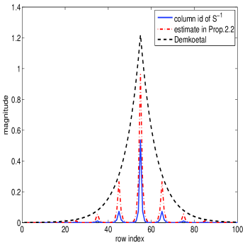
Figure 4: Example 2.1. Values of column t=55𝑑55t=55 of Sβˆ’1superscript𝑆1S^{-1} (solid), estimates for that column as in Prop.2.2 (dashed), and classical bound in [12] (dash-dotted).
Example 2.1.

We consider the symmetric diagonally dominant matrix

M=tridiag​(βˆ’0.5,2Β―,βˆ’0.5)βˆˆβ„10Γ—10.𝑀tridiag0.5Β―20.5superscriptℝ1010M={\rm tridiag}(-0.5,\underline{2},-0.5)\in{\mathbb{R}}^{10\times 10}.

As a sample, we consider column t=55𝑑55t=55 (corresponding to the node at i=5𝑖5i=5 and j=4𝑗4j=4 in the reference grid), and we compute the upper estimate for (Sβˆ’1):,tsubscriptsuperscript𝑆1:𝑑(S^{-1})_{:,t} as the row index varies. Figure 4 shows the accuracy of the estimates in PropositionΒ 2.2 (dashed curve), compared with the actual values (solid curve) of column 55. The estimate is able to capture the highly oscillating decay of the entries of Sβˆ’1superscript𝑆1S^{-1} although, as already mentioned, the peaks are somewhat overestimated. For completeness, the bound (2) from [12] is also reported; for this bound, we took into account that S𝑆S has bandwidth b=n=10𝑏𝑛10b=n=10. We observe that this classical bound provides a good envelope of the actual decay, although, as expected, it misses the oscillation pattern. We also note that the classical bound matches the peaks of our new bound, showing that the classical predicted decay is obtained for either i=ℓ𝑖ℓi=\ell or j=mπ‘—π‘šj=m, corresponding to the rows and columns in the grid most slowing decaying (see also Figure 2).
Refer to caption
Refer to caption
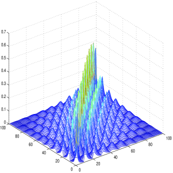
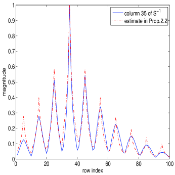
Figure 5: Example 2.2. Left: Components of column t=35𝑑35t=35 of the inverse of the 2D Laplace 100Γ—100100100100\times 100 matrix in the unit square, and its estimate from Proposition 2.2 (all curves are scaled by the values of the corresponding diagonal). Right: upper bounds for all entries of the inverse (cf. with Figure 1)

In the following examples, similar plots are shown, where however all curves are scaled by the value of the corresponding diagonal, so that the maximum value of the column in one.

Example 2.2.

We consider the two-dimensional Laplacian with Dirichlet boundary conditions, discretized by centered finite differences with a 5-point stencil, so that M=tridiag​(βˆ’1,2Β―,βˆ’1)βˆˆβ„10Γ—10𝑀tridiag1Β―21superscriptℝ1010M={\rm tridiag}(-1,\underline{2},-1)\in{\mathbb{R}}^{10\times 10} and S𝑆S is of size 100100100. In Figure 5 we report the values of (Sβˆ’1):,35subscriptsuperscript𝑆1:35(S^{-1})_{:,35} (solid blue line), and those of the corresponding upper bound in Proposition 2.2. The agreement with the actual behavior of the column entries is very good. Similar plots can be observed for the other columns of Sβˆ’1superscript𝑆1S^{-1}.

Example 2.3.

The second example stems from the discretization of the same operator as in Example 2.2, but in terms of the tensorized Babuska-Shen basis, which uses Legendre polynomials. The corresponding symmetric matrix (for even degrees) is given by (see, e.g., [10] and references therein) M=tridiag​(Ξ΄k,Ξ³kΒ―,Ξ΄k)𝑀tridiagsubscriptπ›Ώπ‘˜Β―subscriptπ›Ύπ‘˜subscriptπ›Ώπ‘˜M={\rm tridiag}(\delta_{k},\underline{\gamma_{k}},\delta_{k}), where

Ξ³ksubscriptπ›Ύπ‘˜\displaystyle\gamma_{k} =\displaystyle= 2(4​kβˆ’3)​(4​k+1),k=1,…,n,andformulae-sequence24π‘˜34π‘˜1π‘˜1…𝑛and\displaystyle\frac{2}{(4k-3)(4k+1)},\quad k=1,\ldots,n,\quad{\rm and}
Ξ΄ksubscriptπ›Ώπ‘˜\displaystyle\delta_{k} =\displaystyle= βˆ’1(4​k+1)​(4​kβˆ’1)​(4​k+3),k=1,…,nβˆ’1.formulae-sequence14π‘˜14π‘˜14π‘˜3π‘˜1…𝑛1\displaystyle\frac{-1}{(4k+1)\sqrt{(4k-1)(4k+3)}},\quad k=1,\ldots,n-1.

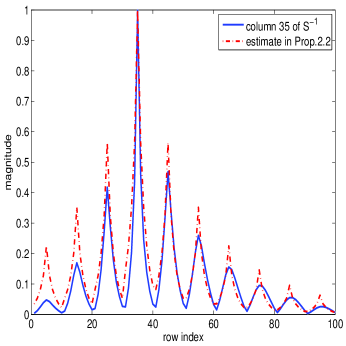
The plot of Figure 6 reports the actual values of (Sβˆ’1):,35subscriptsuperscript𝑆1:35(S^{-1})_{:,35} and their estimates according to Proposition 2.2. Once again, the bounds appear to be fully descriptive of the entry pattern.
Refer to caption
Figure 6: Example 2.3. Components of column t=35𝑑35t=35 of the inverse of the Legendre stiffness matrix of size 100Γ—100100100100\times 100, and its estimate from Proposition 2.2. (all curves are scaled by the values of the corresponding diagonal).

The results of Proposition 2.2 can be manipulated to provide, for each t𝑑t, more explicit estimates on the entries of (Sβˆ’1):,tsubscriptsuperscript𝑆1:𝑑(S^{-1})_{:,t}; more precisely, they are expressed in terms of the β€œ index distance” |β„“βˆ’i|+|mβˆ’j|β„“π‘–π‘šπ‘—|\ell-i|+|m-j|.

Proposition 2.3.

For k,t∈{1,…,n2}π‘˜π‘‘1…superscript𝑛2k,t\in\{1,\ldots,n^{2}\} let j=⌊(tβˆ’1)/nβŒ‹+1,i=tβˆ’nβ€‹βŒŠ(tβˆ’1)/nβŒ‹formulae-sequence𝑗𝑑1𝑛1𝑖𝑑𝑛𝑑1𝑛j=\lfloor(t-1)/n\rfloor+1,i=t-n\lfloor(t-1)/n\rfloor and β„“,mβ„“π‘š\ell,m as in (4).

  1. i)

    Let 𝔫2:=|β„“βˆ’i|+|mβˆ’j|βˆ’2>0assignsubscript𝔫2β„“π‘–π‘šπ‘—20{\mathfrak{n}}_{2}:=|\ell-i|+|m-j|-2>0. If β„“β‰ iℓ𝑖\ell\neq i, mβ‰ jπ‘šπ‘—m\neq j then

    |(Sβˆ’1)k,t|≀12​2​(Ξ»maxβˆ’Ξ»min)𝔫2+2(Ξ»max2+Ξ»min2)𝔫2/2​λmax2+Ξ»min2(Ξ»max​λmin)2​1𝔫2​2​𝔫2𝔫2+4.subscriptsuperscript𝑆1π‘˜π‘‘122superscriptsubscriptπœ†subscriptπœ†subscript𝔫22superscriptsuperscriptsubscriptπœ†2superscriptsubscriptπœ†2subscript𝔫22superscriptsubscriptπœ†2superscriptsubscriptπœ†2superscriptsubscriptπœ†subscriptπœ†21subscript𝔫22subscript𝔫2subscript𝔫24|(S^{-1})_{k,t}|\leq\frac{1}{2\sqrt{2}}\frac{(\lambda_{\max}-\lambda_{\min})^{{\mathfrak{n}}_{2}+2}}{(\lambda_{\max}^{2}+\lambda_{\min}^{2})^{{\mathfrak{n}}_{2}/2}}\frac{\sqrt{\lambda_{\max}^{2}+\lambda_{\min}^{2}}}{(\lambda_{\max}\lambda_{\min})^{2}}\frac{1}{\sqrt{{\mathfrak{n}}_{2}}}\sqrt{\frac{2{\mathfrak{n}}_{2}}{{\mathfrak{n}}_{2}+4}}. (7)
  2. ii)

    Let 𝔫1:=|β„“βˆ’i|+|mβˆ’j|βˆ’1>0assignsubscript𝔫1β„“π‘–π‘šπ‘—10{\mathfrak{n}}_{1}:=|\ell-i|+|m-j|-1>0. If either β„“=iℓ𝑖\ell=i or m=jπ‘šπ‘—m=j and 𝔫1>0subscript𝔫10{\mathfrak{n}}_{1}>0 then

    |(Sβˆ’1)k,t|≀12​2​(Ξ»maxβˆ’Ξ»min)𝔫1+1(Ξ»max2+Ξ»min2)𝔫1/2​λmax2+Ξ»min2Ξ»max​λmin2​1𝔫1​2​𝔫1𝔫1+2.subscriptsuperscript𝑆1π‘˜π‘‘122superscriptsubscriptπœ†subscriptπœ†subscript𝔫11superscriptsuperscriptsubscriptπœ†2superscriptsubscriptπœ†2subscript𝔫12superscriptsubscriptπœ†2superscriptsubscriptπœ†2subscriptπœ†superscriptsubscriptπœ†21subscript𝔫12subscript𝔫1subscript𝔫12|(S^{-1})_{k,t}|\leq\frac{1}{2\sqrt{2}}\frac{(\lambda_{\max}-\lambda_{\min})^{{\mathfrak{n}}_{1}+1}}{(\lambda_{\max}^{2}+\lambda_{\min}^{2})^{{\mathfrak{n}}_{1}/2}}\frac{\sqrt{\lambda_{\max}^{2}+\lambda_{\min}^{2}}}{\lambda_{\max}\lambda_{\min}^{2}}\frac{1}{\sqrt{{\mathfrak{n}}_{1}}}\sqrt{\frac{2{\mathfrak{n}}_{1}}{{\mathfrak{n}}_{1}+2}}. (8)
Proof.

The proof is postponed to the Appendix. ∎

We conclude this paragraph with a final qualitative bound for 𝔫1,𝔫2subscript𝔫1subscript𝔫2{\mathfrak{n}}_{1},{\mathfrak{n}}_{2} large, that emphasizes the asymptotic behavior.

Proposition 2.4.

Let ΞΊ=Ξ»max/Ξ»min=cond​(M)πœ…subscriptπœ†subscriptπœ†cond𝑀\kappa=\lambda_{\max}/\lambda_{\min}={\rm cond}(M).

  1. i)

    Assume β„“,i,m,jβ„“π‘–π‘šπ‘—\ell,i,m,j are such that β„“β‰ iℓ𝑖\ell\neq i, mβ‰ jπ‘šπ‘—m\neq j and 𝔫2=|β„“βˆ’i|+|mβˆ’j|βˆ’2>0subscript𝔫2β„“π‘–π‘šπ‘—20{\mathfrak{n}}_{2}=|\ell-i|+|m-j|-2>0. With the previous notation, it holds

    |(Sβˆ’1)k,t|≀κ2+12​λmin​1𝔫2.subscriptsuperscript𝑆1π‘˜π‘‘superscriptπœ…212subscriptπœ†1subscript𝔫2|(S^{-1})_{k,t}|\leq\frac{\sqrt{\kappa^{2}+1}}{2\lambda_{\min}}\frac{1}{\sqrt{\mathfrak{n}}_{2}}.
  2. ii)

    Assume β„“,i,m,jβ„“π‘–π‘šπ‘—\ell,i,m,j are such that β„“=iℓ𝑖\ell=i or m=jπ‘šπ‘—m=j and 𝔫1=|β„“βˆ’i|+|mβˆ’j|βˆ’1>0subscript𝔫1β„“π‘–π‘šπ‘—10{\mathfrak{n}}_{1}=|\ell-i|+|m-j|-1>0. With the previous notation, it holds

    |(Sβˆ’1)k,t|≀κ​κ2+12​1𝔫1.subscriptsuperscript𝑆1π‘˜π‘‘πœ…superscriptπœ…2121subscript𝔫1|(S^{-1})_{k,t}|\leq\frac{\kappa\sqrt{\kappa^{2}+1}}{2}\frac{1}{\sqrt{\mathfrak{n}}_{1}}.
Proof.

i) The constant involving the extreme eigenvalues of M𝑀M satisfies

(Ξ»maxβˆ’Ξ»min)𝔫+2(Ξ»max2+Ξ»min2)𝔫/2​λmax2+Ξ»min2(Ξ»max​λmin)2≀κ2+1Ξ»min,superscriptsubscriptπœ†subscriptπœ†π”«2superscriptsuperscriptsubscriptπœ†2superscriptsubscriptπœ†2𝔫2superscriptsubscriptπœ†2superscriptsubscriptπœ†2superscriptsubscriptπœ†subscriptπœ†2superscriptπœ…21subscriptπœ†\frac{(\lambda_{\max}-\lambda_{\min})^{{\mathfrak{n}}+2}}{(\lambda_{\max}^{2}+\lambda_{\min}^{2})^{{\mathfrak{n}}/2}}\frac{\sqrt{\lambda_{\max}^{2}+\lambda_{\min}^{2}}}{(\lambda_{\max}\lambda_{\min})^{2}}\leq\frac{\sqrt{\kappa^{2}+1}}{\lambda_{\min}}, (9)

where ΞΊ=Ξ»max/Ξ»minβ‰₯1πœ…subscriptπœ†subscriptπœ†1\kappa=\lambda_{\max}/\lambda_{\min}\geq 1. Indeed,

(Ξ»maxβˆ’Ξ»min)𝔫+2(Ξ»max2+Ξ»min2)𝔫/2​λmax2+Ξ»min2(Ξ»max​λmin)2=Ξ»max𝔫+2Ξ»max𝔫​(1βˆ’1/ΞΊ)𝔫+2(1+1/ΞΊ2)𝔫/2​1Ξ»min2​λmax​1+1ΞΊ2,superscriptsubscriptπœ†subscriptπœ†π”«2superscriptsuperscriptsubscriptπœ†2superscriptsubscriptπœ†2𝔫2superscriptsubscriptπœ†2superscriptsubscriptπœ†2superscriptsubscriptπœ†subscriptπœ†2superscriptsubscriptπœ†π”«2superscriptsubscriptπœ†π”«superscript11πœ…π”«2superscript11superscriptπœ…2𝔫21superscriptsubscriptπœ†2subscriptπœ†11superscriptπœ…2\displaystyle\frac{(\lambda_{\max}-\lambda_{\min})^{{\mathfrak{n}}+2}}{(\lambda_{\max}^{2}+\lambda_{\min}^{2})^{{\mathfrak{n}}/2}}\frac{\sqrt{\lambda_{\max}^{2}+\lambda_{\min}^{2}}}{(\lambda_{\max}\lambda_{\min})^{2}}=\frac{\lambda_{\max}^{{\mathfrak{n}}+2}}{\lambda_{\max}^{\mathfrak{n}}}\frac{(1-1/\kappa)^{{\mathfrak{n}}+2}}{(1+1/\kappa^{2})^{{\mathfrak{n}}/2}}\frac{1}{\lambda_{\min}^{2}\lambda_{\max}}\sqrt{1+\frac{1}{\kappa^{2}}},

with (1βˆ’1/ΞΊ)𝔫+2(1+1/ΞΊ2)𝔫/2≀1superscript11πœ…π”«2superscript11superscriptπœ…2𝔫21\frac{(1-1/\kappa)^{{\mathfrak{n}}+2}}{(1+1/\kappa^{2})^{{\mathfrak{n}}/2}}\leq 1. Inserting (9) into (7) and noticing that 𝔫2𝔫2/2+1≀2subscript𝔫2subscript𝔫2212\frac{{\mathfrak{n}}_{2}}{{\mathfrak{n}}_{2}/2+1}\leq 2 yield the result.

The proof of ii) goes along the same lines of i) after observing that it holds

(Ξ»maxβˆ’Ξ»min)𝔫+2(Ξ»max2+Ξ»min2)𝔫/2​λmax2+Ξ»min2Ξ»max​λmin2≀λmax​κ2+1Ξ»min=κ​κ2+1.superscriptsubscriptπœ†subscriptπœ†π”«2superscriptsuperscriptsubscriptπœ†2superscriptsubscriptπœ†2𝔫2superscriptsubscriptπœ†2superscriptsubscriptπœ†2subscriptπœ†superscriptsubscriptπœ†2subscriptπœ†superscriptπœ…21subscriptπœ†πœ…superscriptπœ…21\frac{(\lambda_{\max}-\lambda_{\min})^{{\mathfrak{n}}+2}}{(\lambda_{\max}^{2}+\lambda_{\min}^{2})^{{\mathfrak{n}}/2}}\frac{\sqrt{\lambda_{\max}^{2}+\lambda_{\min}^{2}}}{\lambda_{\max}\lambda_{\min}^{2}}\leq\frac{\lambda_{\max}\sqrt{\kappa^{2}+1}}{\lambda_{\min}}=\kappa\sqrt{\kappa^{2}+1}.

∎

We remark that a result in a similar direction was reported in [19, Theorem 4.5] for the Laplacian matrix, although in there, an explicit dependence on the problem dimension arises, together with a more involved dependence on the discretization grid.

In terms of the indices of Sβˆ’1superscript𝑆1S^{-1}, our bound shows that

|(Sβˆ’1)k,t|subscriptsuperscript𝑆1π‘˜π‘‘\displaystyle|(S^{-1})_{k,t}| =\displaystyle= |(Sβˆ’1)β„“+n​(mβˆ’1),i+n​(jβˆ’1)|subscriptsuperscript𝑆1β„“π‘›π‘š1𝑖𝑛𝑗1\displaystyle|(S^{-1})_{\ell+n(m-1),i+n(j-1)}|
≀\displaystyle\leq Ξ³0​1|β„“βˆ’i|+|mβˆ’j|βˆ’2subscript𝛾01β„“π‘–π‘šπ‘—2\displaystyle\gamma_{0}\frac{1}{\sqrt{|\ell-i|+|m-j|-2}}
=\displaystyle= Ξ³0​1|kβˆ’tβˆ’n​(⌊(kβˆ’1)nβŒ‹βˆ’βŒŠ(tβˆ’1)nβŒ‹)|+|⌊(kβˆ’1)nβŒ‹βˆ’βŒŠ(tβˆ’1)nβŒ‹|βˆ’2.subscript𝛾01π‘˜π‘‘π‘›π‘˜1𝑛𝑑1π‘›π‘˜1𝑛𝑑1𝑛2\displaystyle\gamma_{0}\frac{1}{\sqrt{|k-t-n(\lfloor\frac{(k-1)}{n}\rfloor-\lfloor\frac{(t-1)}{n}\rfloor)|+|\lfloor\frac{(k-1)}{n}\rfloor-\lfloor\frac{(t-1)}{n}\rfloor|-2}}.

For instance, for all the elements on the secondary diagonal, satisfying k+t=n2π‘˜π‘‘superscript𝑛2k+t=n^{2}, we obtain

|(Sβˆ’1)k,t|≀γ0​1(|n2βˆ’2​tβˆ’n​(⌊n2βˆ’tβˆ’1nβŒ‹βˆ’βŒŠtβˆ’1nβŒ‹)|+|⌊n2βˆ’tβˆ’1nβŒ‹βˆ’βŒŠtβˆ’1nβŒ‹|βˆ’2)12.subscriptsuperscript𝑆1π‘˜π‘‘subscript𝛾01superscriptsuperscript𝑛22𝑑𝑛superscript𝑛2𝑑1𝑛𝑑1𝑛superscript𝑛2𝑑1𝑛𝑑1𝑛212|(S^{-1})_{k,t}|\leq\gamma_{0}\frac{1}{(|n^{2}-2t-n(\lfloor\frac{n^{2}-t-1}{n}\rfloor-\lfloor\frac{t-1}{n}\rfloor)|+|\lfloor\frac{n^{2}-t-1}{n}\rfloor-\lfloor\frac{t-1}{n}\rfloor|-2)^{\frac{1}{2}}}.

In the qualitative bound of Proposition 2.4 the asymptotic term does not depend on the actual entries of Sβˆ’1superscript𝑆1S^{-1}, but only on the position in the underlying grid. This property reflects similar considerations obtained for point-wise estimates in the context of the discrete Laplacian. Indeed, for the discrete Green function GhsubscriptπΊβ„ŽG_{h} on the discrete N𝑁N-dimensional grid Rhsubscriptπ‘…β„ŽR_{h}, it was shown in [9] that there exist constants h0subscriptβ„Ž0h_{0} and C𝐢C such that for h≀h0β„Žsubscriptβ„Ž0h\leq h_{0}, x,y∈Rhπ‘₯𝑦subscriptπ‘…β„Žx,y\in R_{h},

Gh​(x,y)≀{C​log⁑C|xβˆ’y|+hif​N=2C(|xβˆ’y|+h)Nβˆ’2if​Nβ‰₯3.subscriptπΊβ„Žπ‘₯𝑦cases𝐢𝐢π‘₯π‘¦β„Žif𝑁2𝐢superscriptπ‘₯π‘¦β„Žπ‘2if𝑁3\displaystyle G_{h}(x,y)\leq\left\{\begin{array}[]{ll}C\log\frac{C}{|x-y|+h}&{\rm if}N=2\\ \frac{C}{(|x-y|+h)^{N-2}}&{\rm if}N\geq 3.\end{array}\right. (12)

Our computable bound in PropositionΒ 2.4 shows that the entries depend on the inverse square root of the distance, whereas in (12) an asymptotic (slower) logarithmic dependence on the distance is reported for the two-dimensional case.

We also notice that other bounds are available that use different distance concepts; for instance, in [7, Theorem 3.4] the decay pattern of certain matrix functions is described by means of graph theory, in terms of distance111Defined as the length of the shortest directed path connecting the two nodes. between nodes of a digraph, where the nodes are the entry indices in the matrix inverse.

3 On the decay of the Cholesky factor

When preconditioning a large algebraic linear system, a-priori information on the decay properties of the inverse of the Cholesky factor of S𝑆S may be important to guide the computation of incomplete factorizations. Indeed, assuming that S=L​LβŠ€π‘†πΏsuperscript𝐿topS=LL^{\top} is the Cholesky factorization of S𝑆S, if the entries of Sβˆ’1superscript𝑆1S^{-1} decay away from the main diagonal with a certain pattern, we expect that also the factor inverse Lβˆ’βŠ€superscript𝐿absenttopL^{-\top} will show a similar pattern. This fact was proved in [8] for banded matrices S𝑆S by using the decay rate in (2). With the same technical tools, we generalize this result to our decay pattern, under the assumption that S𝑆S has a bandwidth b𝑏b.

Proposition 3.1.

Assume S𝑆S is b𝑏b-banded, with diagonal elements not greater than one, and let S=L​LβŠ€π‘†πΏsuperscript𝐿topS=LL^{\top}. With the previous notation, for 𝔫=𝔫i>0𝔫subscript𝔫𝑖0{\mathfrak{n}}={\mathfrak{n}}_{i}>0, i=1,2𝑖12i=1,2,

|(Lβˆ’βŠ€)k,t|≀γ0​b𝔫​(k,t).subscriptsuperscript𝐿absenttopπ‘˜π‘‘subscript𝛾0π‘π”«π‘˜π‘‘|(L^{-\top})_{k,t}|\leq\gamma_{0}\frac{b}{\sqrt{\mathfrak{n}(k,t)}}.
Proof.

We have

|(Lβˆ’βŠ€)k,t|β‰€βˆ‘r=tt+bβˆ’1|(Sβˆ’1)k,r|​|Lr,t|≀γ0β€‹βˆ‘r=tt+bβˆ’11𝔫​(k,r)≀γ0​b𝔫​(k,t),subscriptsuperscript𝐿absenttopπ‘˜π‘‘superscriptsubscriptπ‘Ÿπ‘‘π‘‘π‘1subscriptsuperscript𝑆1π‘˜π‘ŸsubscriptπΏπ‘Ÿπ‘‘subscript𝛾0superscriptsubscriptπ‘Ÿπ‘‘π‘‘π‘11π”«π‘˜π‘Ÿsubscript𝛾0π‘π”«π‘˜π‘‘|(L^{-\top})_{k,t}|\leq\sum_{r=t}^{t+b-1}|(S^{-1})_{k,r}|\,|L_{r,t}|\leq\gamma_{0}\sum_{r=t}^{t+b-1}\frac{1}{\sqrt{\mathfrak{n}(k,r)}}\leq\gamma_{0}\frac{b}{\sqrt{\mathfrak{n}(k,t)}},

where we used the inequality 𝔫​(k,t)≀𝔫​(k,r)π”«π‘˜π‘‘π”«π‘˜π‘Ÿ{\mathfrak{n}(k,t)}\leq{\mathfrak{n}(k,r)} for k≀t≀r≀t+bβˆ’1π‘˜π‘‘π‘Ÿπ‘‘π‘1k\leq t\leq r\leq t+b-1. ∎

We notice that a slightly sharper upper bound could be obtained by first using the bound of PropositionΒ 2.2, however the final asymptotic dependence with respect to 𝔫𝔫\mathfrak{n} would still be the same.

The estimate for the entries of Lβˆ’1superscript𝐿1L^{-1} could be used in the design of linear system preconditioners by means of approximate inverses [8],[2]. Indeed, not only a decay pattern occurs away from the diagonal, but many tiny values appear within the bandwidth. Therefore, a threshold-based dropping strategy could be used in conjunction with a band-based procedure, to a-priori increase the sparsity of the explicit approximate inverse. Similar considerations can guide the design of quasi-orthogonal polynomial bases, as those developed in, e.g., [10],[11].

4 More general settings

The results of the previous sections can be generalized in a number of ways. For instance, we can allow the symmetric and positive matrix M𝑀M in (1) to be generally b𝑏b-banded, so that PropositionΒ 2.1 can be used in its full generality. The resulting estimate is reported below. Its proof is omitted as it is analogous to that of Proposition 2.2.

Proposition 4.1.

Let M𝑀M be a real symmetric and positive definite matrix of size n𝑛n and bandwidth b𝑏b. For k,t∈{1,…,n2}π‘˜π‘‘1…superscript𝑛2k,t\in\{1,\ldots,n^{2}\}, let

j=⌊(tβˆ’1)/nβŒ‹+1,i=tβˆ’nβ€‹βŒŠ(tβˆ’1)/nβŒ‹formulae-sequence𝑗𝑑1𝑛1𝑖𝑑𝑛𝑑1𝑛j=\lfloor(t-1)/n\rfloor+1,\quad i=t-n\lfloor(t-1)/n\rfloor

and β„“,mβ„“π‘š\ell,m as in (4). With the notation above, the following holds.

i) If i≠ℓ𝑖ℓi\neq\ell and jβ‰ mπ‘—π‘šj\neq m, then

|(Sβˆ’1)k,t|≀12​π​64|Ξ»maxβˆ’Ξ»min|2β€‹βˆ«βˆ’βˆžβˆž(R2(R2βˆ’1)2)2​(1R)|iβˆ’β„“|/b+|jβˆ’m|/bβˆ’2​dΟ‰;subscriptsuperscript𝑆1π‘˜π‘‘12πœ‹64superscriptsubscriptπœ†subscriptπœ†2superscriptsubscriptsuperscriptsuperscript𝑅2superscriptsuperscript𝑅2122superscript1π‘…π‘–β„“π‘π‘—π‘šπ‘2differential-dπœ”|(S^{-1})_{k,t}|\leq\frac{1}{2\pi}\frac{64}{|\lambda_{\max}-\lambda_{\min}|^{2}}\int_{-\infty}^{\infty}\left(\frac{R^{2}}{(R^{2}-1)^{2}}\right)^{2}\left(\frac{1}{R}\right)^{|i-\ell|/b+|j-m|/b-2}{\rm d}\omega;

ii) If either i=ℓ𝑖ℓi=\ell or j=mπ‘—π‘šj=m, then

|(Sβˆ’1)k,t|≀12​π​8|Ξ»maxβˆ’Ξ»min|β€‹βˆ«βˆ’βˆžβˆž1Ξ»min2+Ο‰2​R2(R2βˆ’1)2​(1R)|iβˆ’β„“|/b+|jβˆ’m|/bβˆ’1​dΟ‰;subscriptsuperscript𝑆1π‘˜π‘‘12πœ‹8subscriptπœ†subscriptπœ†superscriptsubscript1superscriptsubscriptπœ†2superscriptπœ”2superscript𝑅2superscriptsuperscript𝑅212superscript1π‘…π‘–β„“π‘π‘—π‘šπ‘1differential-dπœ”|(S^{-1})_{k,t}|\leq\frac{1}{2\pi}\frac{8}{|\lambda_{\max}-\lambda_{\min}|}\int_{-\infty}^{\infty}\frac{1}{\sqrt{\lambda_{\min}^{2}+\omega^{2}}}\frac{R^{2}}{(R^{2}-1)^{2}}\left(\frac{1}{R}\right)^{|i-\ell|/b+|j-m|/b-1}{\rm d}\omega;

iii) If both i=ℓ𝑖ℓi=\ell and j=mπ‘—π‘šj=m, then

|(Sβˆ’1)k,t|≀12β€‹Ο€β€‹βˆ«βˆ’βˆžβˆž1Ξ»min2+Ο‰2​dΟ‰=12​λmin.subscriptsuperscript𝑆1π‘˜π‘‘12πœ‹superscriptsubscript1superscriptsubscriptπœ†2superscriptπœ”2differential-dπœ”12subscriptπœ†|(S^{-1})_{k,t}|\leq\frac{1}{2\pi}\int_{-\infty}^{\infty}\frac{1}{\lambda_{\min}^{2}+\omega^{2}}{\rm d}\omega=\frac{1}{2\lambda_{\min}}.
Refer to caption
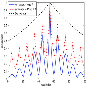
Figure 7: Example 4.1. Components of column t=55𝑑55t=55 of the inverse of the Laplace stiffness matrix of size 100Γ—100100100100\times 100 with a 9-point stencil discretization, and its estimate from Proposition 4.1. (all curves are scaled by the values of the corresponding diagonal.)
Example 4.1.

We consider the 100Γ—100100100100\times 100 matrix S𝑆S stemming from the discretization of the two-dimensional Laplace operator by means of a more accurate discretization (9-point stencil) of the one-dimensional derivative than in Example 2.2. This gives

M=pentadiag​(112,βˆ’43,156Β―,βˆ’43,112),𝑀pentadiag11243Β―15643112M={\rm pentadiag}\left(\frac{1}{12},-\frac{4}{3},\underline{\frac{15}{6}},-\frac{4}{3},\frac{1}{12}\right),

which has bandwidth b=2𝑏2b=2. The plot in Figure 7 (for column t=55𝑑55t=55 of the inverse Sβˆ’1superscript𝑆1S^{-1}) shows that the estimate of PropositionΒ 4.1 is able to capture the oscillating behavior, but somewhat fails to follow the asymptotic pattern of the inverse, predicting a slower decay. (We recall here that all values were scaled to be one at the t𝑑t-th component.) As already mentioned, this seems to be due to the weakness of the exponential bound in Proposition 2.1 for a larger bandwidth. We explicitly observe that also the monotonic classical bound (2) does not seem to closely match the actual asymptotic decay pattern; we should keep in mind that in this case, S𝑆S has bandwidth bβ‹…n=20⋅𝑏𝑛20b\cdot n=20, which seems to also significantly deteriorate the classical estimate.

Another generalization is obtained by assuming that S=Sg𝑆subscript𝑆𝑔S=S_{g} can be written as in (3), with M1subscript𝑀1M_{1}, M2subscript𝑀2M_{2} symmetric and positive definite square matrices, of size n1subscript𝑛1n_{1} and n2subscript𝑛2n_{2}, respectively, so that Sgsubscript𝑆𝑔S_{g} is of size n1​n2Γ—n1​n2subscript𝑛1subscript𝑛2subscript𝑛1subscript𝑛2n_{1}n_{2}\times n_{1}n_{2}. Following the derivation in SectionΒ 2, the elements of each column t𝑑t of the inverse can be derived as the elements of the solution matrix 𝒳𝒳{\cal X} to the Sylvester equation

M1​𝒳+𝒳​M2=β„°.subscript𝑀1𝒳𝒳subscript𝑀2β„°\displaystyle M_{1}{\cal X}+{\cal X}M_{2}={\cal E}. (13)

The following result generalizes one of the cases of Proposition 2.2. The other case can be derived analogously.

Proposition 4.2.

Assume M1,M2subscript𝑀1subscript𝑀2M_{1},M_{2} are symmetric positive definite and tridiagonal matrices. Let Ξ΄1,2=(Ξ»max​(M1)βˆ’Ξ»min​(M1))​(Ξ»max​(M2)βˆ’Ξ»min​(M2))subscript𝛿12subscriptπœ†subscript𝑀1subscriptπœ†subscript𝑀1subscriptπœ†subscript𝑀2subscriptπœ†subscript𝑀2\delta_{1,2}=(\lambda_{\max}(M_{1})-\lambda_{\min}(M_{1}))(\lambda_{\max}(M_{2})-\lambda_{\min}(M_{2})). For k,t∈{1,…,n1​n2}π‘˜π‘‘1…subscript𝑛1subscript𝑛2k,t\in\{1,\ldots,n_{1}n_{2}\} let j=⌊(tβˆ’1)/n1βŒ‹+1,i=tβˆ’n1β€‹βŒŠ(tβˆ’1)/n1βŒ‹formulae-sequence𝑗𝑑1subscript𝑛11𝑖𝑑subscript𝑛1𝑑1subscript𝑛1j=\lfloor(t-1)/n_{1}\rfloor+1,\quad i=t-n_{1}\lfloor(t-1)/n_{1}\rfloor, β„“=⌊(kβˆ’1)/n1βŒ‹+1,m=tβˆ’n1β€‹βŒŠ(kβˆ’1)/n1βŒ‹formulae-sequenceβ„“π‘˜1subscript𝑛11π‘šπ‘‘subscript𝑛1π‘˜1subscript𝑛1\ell=\lfloor(k-1)/n_{1}\rfloor+1,\quad m=t-n_{1}\lfloor(k-1)/n_{1}\rfloor, be such that β„“β‰ iℓ𝑖\ell\neq i and mβ‰ jπ‘šπ‘—m\neq j. Then it holds that

|(Sgβˆ’1)k,t|≀12​π​64Ξ΄1,2β€‹βˆ«βˆ’βˆžβˆžR12(R12βˆ’1)2​R22(R22βˆ’1)2​(1R1)|iβˆ’β„“|βˆ’1​(1R2)|jβˆ’m|βˆ’1​dΟ‰,subscriptsuperscriptsubscript𝑆𝑔1π‘˜π‘‘12πœ‹64subscript𝛿12superscriptsubscriptsuperscriptsubscript𝑅12superscriptsuperscriptsubscript𝑅1212superscriptsubscript𝑅22superscriptsuperscriptsubscript𝑅2212superscript1subscript𝑅1𝑖ℓ1superscript1subscript𝑅2π‘—π‘š1differential-dπœ”|(S_{g}^{-1})_{k,t}|\leq\frac{1}{2\pi}\frac{64}{\delta_{1,2}}\int_{-\infty}^{\infty}\frac{R_{1}^{2}}{(R_{1}^{2}-1)^{2}}\frac{R_{2}^{2}}{(R_{2}^{2}-1)^{2}}\left(\frac{1}{R_{1}}\right)^{|i-\ell|-1}\left(\frac{1}{R_{2}}\right)^{|j-m|-1}{\rm d}\omega,

with R1subscript𝑅1R_{1} and R2subscript𝑅2R_{2} are defined as in Proposition 2.1 for each of the spectra of M1subscript𝑀1M_{1} and M2subscript𝑀2M_{2}, respectively.

Proof.

We can write the solution to the Sylvester equation in closed form as (see, e.g., [15])

𝒳tsubscript𝒳𝑑\displaystyle{\cal X}_{t} =\displaystyle= 12β€‹Ο€β€‹βˆ«βˆ’βˆžβˆž(ı​ω​I+M1)βˆ’1​ei​ejβŠ€β€‹(ı​ω​I+M2)βˆ’βˆ—β€‹dΟ‰.12πœ‹superscriptsubscriptsuperscriptitalic-Δ±πœ”πΌsubscript𝑀11subscript𝑒𝑖superscriptsubscript𝑒𝑗topsuperscriptitalic-Δ±πœ”πΌsubscript𝑀2absentdifferential-dπœ”\displaystyle\frac{1}{2\pi}\int_{-\infty}^{\infty}(\imath\omega I+M_{1})^{-1}e_{i}e_{j}^{\top}(\imath\omega I+M_{2})^{-*}{\rm d}\omega.

To evaluate |(𝒳t)β„“,m|subscriptsubscriptπ’³π‘‘β„“π‘š|({\cal X}_{t})_{\ell,m}| we can then apply again PropositionΒ 2.1 to each of the inner term, namely to |eβ„“βŠ€β€‹(ı​ω​I+M1)βˆ’βˆ—β€‹ei|superscriptsubscript𝑒ℓtopsuperscriptitalic-Δ±πœ”πΌsubscript𝑀1absentsubscript𝑒𝑖|e_{\ell}^{\top}(\imath\omega I+M_{1})^{-*}e_{i}|, |ejβŠ€β€‹(ı​ω​I+M2)βˆ’βˆ—β€‹em|superscriptsubscript𝑒𝑗topsuperscriptitalic-Δ±πœ”πΌsubscript𝑀2absentsubscriptπ‘’π‘š|e_{j}^{\top}(\imath\omega I+M_{2})^{-*}e_{m}|. The final result thus follows as in Proposition 2.2. ∎

Finally, we observe that the two generalizations above could be combined, giving estimates for the entries of the inverse when M1subscript𝑀1M_{1} and M2subscript𝑀2M_{2} have different bandwidth.

5 Conclusions

We have characterized the decay pattern of the inverse of banded matrices that can be written as the sum of two Kronecker products, in which each of the matrices is symmetric positive definite and banded. Our results explain the non-monotonic (oscillating) pattern commonly observed in these inverses, while providing upper bounds that can be sharp, especially for low bandwidth. We also showed that corresponding results can be obtained for more general Kronecker-type matrices with different banded matrices M1subscript𝑀1M_{1} and M2subscript𝑀2M_{2}.

Acknowledgements

The authors would like to thank Leonid Knizhnerman for carefully reading an earlier draft of this manuscript, and Michele Benzi for helpful discussions. The first and third authors were partially supported by the Italian research fund INdAM-GNCS 2013 β€œAspetti emergenti nello studio di strategie adattative per problemi differenziali”. The second author was partially supported by the University of Bologna through the FARB Project β€œMetodi matematici per l’esplorazione ambientale sostenibile”.

References

  • [1] M. Bebendorf and W. Hackbusch. Existence of β„‹β„‹{\mathcal{H}}-matrix approximants to the inverse FE-matrix of elliptic operators with L∞superscript𝐿L^{\infty} -coefficients. Numer. Math., 95:1–28, 2003.
  • [2] M.Β Benzi. Preconditioning techniques for large linear systems: a survey. J. Comput. Phys, 182:418–477, 2002.
  • [3] M.Β Benzi and P.Β Boito. Quadrature rule-based bounds for functions of adjacency matrices. Lin. Alg. Appl., 433:637–652, 2010.
  • [4] M.Β Benzi and P.Β Boito. Decay properties for functions of matrices over Cβˆ—superscript𝐢C^{*} -algebras. Lin. Alg. Appl., xx:xx, 2013.
  • [5] M.Β Benzi, P.Β Boito, and N.Β Razouk. Decay properties of spectral projectors with applications to electronic structure. SIAM Review, 55:3–64, 2013.
  • [6] M.Β Benzi and G.Β H. Golub. Bounds for the entries of matrix functions with applications to preconditioning. BIT Numerical Mathematics, 39(3):417–438, 1999.
  • [7] M.Β Benzi and N.Β Razouk. Decay bounds and O​(n)𝑂𝑛O(n) algorithms for approximating functions of sparse matrices. ETNA, 28:16–39, 2007.
  • [8] M.Β Benzi and M.Β Tuma. Orderings fo factorized sparse approximate inverse preconditioners. SIAM J. Sci. Comput., 21(5):1851–1868, 2000.
  • [9] J.Β H. Bramble and V.Β ThomΓ©e. Pointwise bounds for discrete Green’s functions. SIAM Journal on Numerical Analysis, 6(4):583–590, Dec. 1969.
  • [10] C.Β Canuto, V.Β Simoncini, and M.Β Verani. Adaptive Legendre-Galerkin methods, 2014. In preparation.
  • [11] M. Challacombe. A simplified density matrix minimization for linear scaling self-consistent field theory. J. Chem. Phys., 110:2332–2342, 1999.
  • [12] S.Β Demko, W.Β F. Moss, and P.Β W. Smith. Decay rates for inverses of band matrices. Math. Comp., 43:491–499, 1984.
  • [13] R.Β Freund. On polynomial approximations to fa​(z)=(zβˆ’a)βˆ’1subscriptπ‘“π‘Žπ‘§superscriptπ‘§π‘Ž1f_{a}(z)=(z-a)^{-1} with complex aπ‘Ža and some applications to certain non-hermitian matrices. Approx. Theory and Appl., 5:15–31, 1989.
  • [14] I.Β S. Gradshteyn and I.Β M. Ryzhik. Table of integrals, series, and products. Corrected and enlarged edition. Academic Press, San Diego, California, 1980.
  • [15] R.Β A. Horn and C.Β R. Johnson. Topics in Matrix Analysis. Cambridge University Press, Cambridge, 1991.
  • [16] R.Β J. LeVeque. Finite Difference Methods for Ordinary and Partial Differential Equations. Steady State and Time Dependent Problems. SIAM, Philadelphia, 2007.
  • [17] P.E. Maslen, C.Β Ochsenfeld, C.Β A. White, M.Β S. Lee, and M.Β Head-Gordon. Locality and Sparsity of Ab Initio One-Particle Density Matrices and Localized Orbitals. J. Phys. Chem. A, 102:2215–2222, 1998.
  • [18] G.Β T. McAllister and E.Β F. Sabotka. Discrete Green’s functions. Math. Comp., 27:59–80, 1973.
  • [19] G.Β Meurant. A review on the inverse of symmetric tridiagonal and block tridiagonal matrices. SIAM J. Matrix Anal. Appl., 13(3):707–728, Jul. 1992.
  • [20] R.Β Nabben. Decay rates of the inverse of nonsymmetric tridiagonal and band matrices. SIAM J. Matrix Anal. Appl., 20:820–837, 1999.
  • [21] R.Β Vandebril, M.Β Van Barel, and N.Β Mastronardi. Matrix computations and semiseparable matrices. Johns Hopkins University Press, 2008.
  • [22] T.Β Vejchodsky and P.Β Solin. Discrete maximum principle for higher-order finite elements in 1D. Math. Comp, 76(260):1833–1846, October 2007.
  • [23] P.Β Wojtaszczyk. A mathematical introduction to Wavelets. Cambridge University Press, 1997.

Appendix

In this appendix we prove Proposition 2.3.

Proof.

i) We set 𝒳ℓ​m:=eβ„“βŠ€β€‹π’³t​em=(Sβˆ’1)k,tassignsubscriptπ’³β„“π‘šsuperscriptsubscript𝑒ℓtopsubscript𝒳𝑑subscriptπ‘’π‘šsubscriptsuperscript𝑆1π‘˜π‘‘{\cal X}_{\ell m}:=e_{\ell}^{\top}{\cal X}_{t}e_{m}=(S^{-1})_{k,t}. From the result of Proposition 2.2, we need to bound the integrand in a way that the integral still converges.

We observe that

1R≀1Ξ±1𝑅1𝛼\displaystyle\frac{1}{R}\leq\frac{1}{\alpha} =\displaystyle= Ξ»maxβˆ’Ξ»min|Ξ»1|+|Ξ»2|subscriptπœ†subscriptπœ†subscriptπœ†1subscriptπœ†2\displaystyle\frac{\lambda_{\max}-\lambda_{\min}}{|\lambda_{1}|+|\lambda_{2}|}
≀\displaystyle\leq Ξ»maxβˆ’Ξ»min(Ξ»max2+Ξ»min2+2​ω2)1/2=Ξ»maxβˆ’Ξ»min(Ξ»max2+Ξ»min2)1/2​1(1+2​ω2Ξ»max2+Ξ»min2)1/2.subscriptπœ†subscriptπœ†superscriptsuperscriptsubscriptπœ†2superscriptsubscriptπœ†22superscriptπœ”212subscriptπœ†subscriptπœ†superscriptsuperscriptsubscriptπœ†2superscriptsubscriptπœ†2121superscript12superscriptπœ”2superscriptsubscriptπœ†2superscriptsubscriptπœ†212\displaystyle\frac{\lambda_{\max}-\lambda_{\min}}{(\lambda_{\max}^{2}+\lambda_{\min}^{2}+2\omega^{2})^{1/2}}=\frac{\lambda_{\max}-\lambda_{\min}}{(\lambda_{\max}^{2}+\lambda_{\min}^{2})^{1/2}}\frac{1}{\left(1+\frac{2\omega^{2}}{\lambda_{\max}^{2}+\lambda_{\min}^{2}}\right)^{1/2}}.

Moreover, after some algebraic calculation, it follows that Rβˆ’1/R=2​α2βˆ’1𝑅1𝑅2superscript𝛼21R-1/R=2\sqrt{\alpha^{2}-1}, and since Ξ±2βˆ’1β‰₯(2​ω2+2​λmax​λmin)/(Ξ»maxβˆ’Ξ»min)2superscript𝛼212superscriptπœ”22subscriptπœ†subscriptπœ†superscriptsubscriptπœ†subscriptπœ†2\alpha^{2}-1\geq(2\omega^{2}+2\lambda_{\max}\lambda_{\min})/(\lambda_{\max}-\lambda_{\min})^{2},

R2(R2βˆ’1)2=14​(Ξ±2βˆ’1)≀18​|Ξ»maxβˆ’Ξ»min|2Ο‰2+Ξ»max​λmin.superscript𝑅2superscriptsuperscript𝑅21214superscript𝛼2118superscriptsubscriptπœ†subscriptπœ†2superscriptπœ”2subscriptπœ†subscriptπœ†\displaystyle\frac{R^{2}}{(R^{2}-1)^{2}}=\frac{1}{4(\alpha^{2}-1)}\leq\frac{1}{8}\frac{|\lambda_{\max}-\lambda_{\min}|^{2}}{\omega^{2}+\lambda_{\max}\lambda_{\min}}. (14)

Therefore, letting 𝔫2=|iβˆ’β„“|+|jβˆ’m|βˆ’2subscript𝔫2π‘–β„“π‘—π‘š2{{\mathfrak{n}}_{2}}={|i-\ell|+|j-m|-2},

|𝒳ℓ​m|subscriptπ’³β„“π‘š\displaystyle|{\cal X}_{\ell m}| ≀\displaystyle\leq 12​π​64|Ξ»maxβˆ’Ξ»min|2β€‹βˆ«βˆ’βˆžβˆž(R2(R2βˆ’1)2)2​(1R)𝔫2​dΟ‰12πœ‹64superscriptsubscriptπœ†subscriptπœ†2superscriptsubscriptsuperscriptsuperscript𝑅2superscriptsuperscript𝑅2122superscript1𝑅subscript𝔫2differential-dπœ”\displaystyle\frac{1}{2\pi}\frac{64}{|{\lambda_{\max}-\lambda_{\min}}|^{2}}\int_{-\infty}^{\infty}\left(\frac{R^{2}}{(R^{2}-1)^{2}}\right)^{2}\left(\frac{1}{R}\right)^{{\mathfrak{n}}_{2}}{\rm d}\omega
≀\displaystyle\leq 12​π​64​|Ξ»maxβˆ’Ξ»min|464​|Ξ»maxβˆ’Ξ»min|2​(Ξ»maxβˆ’Ξ»min(Ξ»max2+Ξ»min2)12)𝔫2β€‹βˆ«βˆ’βˆžβˆž1(Ο‰2+Ξ»max​λmin)2​(11+2​ω2Ξ»max2+Ξ»min2)𝔫22​dΟ‰12πœ‹64superscriptsubscriptπœ†subscriptπœ†464superscriptsubscriptπœ†subscriptπœ†2superscriptsubscriptπœ†subscriptπœ†superscriptsuperscriptsubscriptπœ†2superscriptsubscriptπœ†212subscript𝔫2superscriptsubscript1superscriptsuperscriptπœ”2subscriptπœ†subscriptπœ†2superscript112superscriptπœ”2superscriptsubscriptπœ†2superscriptsubscriptπœ†2subscript𝔫22differential-dπœ”\displaystyle\frac{1}{2\pi}\frac{64|\lambda_{\max}-\lambda_{\min}|^{4}}{{64}|\lambda_{\max}-\lambda_{\min}|^{2}}\left(\frac{\lambda_{\max}-\lambda_{\min}}{(\lambda_{\max}^{2}+\lambda_{\min}^{2})^{\frac{1}{2}}}\right)^{{\mathfrak{n}}_{2}}\int_{-\infty}^{\infty}\frac{1}{(\omega^{2}+\lambda_{\max}\lambda_{\min})^{2}}\left(\frac{1}{1+\frac{2\omega^{2}}{\lambda_{\max}^{2}+\lambda_{\min}^{2}}}\right)^{\frac{{\mathfrak{n}}_{2}}{2}}{\rm d}\omega
≀\displaystyle\leq 12​π​(Ξ»maxβˆ’Ξ»min)𝔫2+2(Ξ»max2+Ξ»min2)𝔫22β€‹βˆ«βˆ’βˆžβˆž1(Ο‰2+Ξ»max​λmin)2​(11+2​ω2Ξ»max2+Ξ»min2)𝔫22​dΟ‰.12πœ‹superscriptsubscriptπœ†subscriptπœ†subscript𝔫22superscriptsuperscriptsubscriptπœ†2superscriptsubscriptπœ†2subscript𝔫22superscriptsubscript1superscriptsuperscriptπœ”2subscriptπœ†subscriptπœ†2superscript112superscriptπœ”2superscriptsubscriptπœ†2superscriptsubscriptπœ†2subscript𝔫22differential-dπœ”\displaystyle\frac{1}{2\pi}\frac{(\lambda_{\max}-\lambda_{\min})^{{{\mathfrak{n}}_{2}}+2}}{(\lambda_{\max}^{2}+\lambda_{\min}^{2})^{\frac{{\mathfrak{n}}_{2}}{2}}}\int_{-\infty}^{\infty}\frac{1}{(\omega^{2}+\lambda_{\max}\lambda_{\min})^{2}}\left(\frac{1}{1+\frac{2\omega^{2}}{\lambda_{\max}^{2}+\lambda_{\min}^{2}}}\right)^{\frac{{\mathfrak{n}}_{2}}{2}}{\rm d}\omega.

Since

1Ο‰2+Ξ»max​λmin=1Ξ»max​λmin​12​ω22​λmin​λ​max+1≀1Ξ»max​λmin​12​ω2Ξ»min2+Ξ»max2+1,1superscriptπœ”2subscriptπœ†subscriptπœ†1subscriptπœ†subscriptπœ†12superscriptπœ”22subscriptπœ†πœ†11subscriptπœ†subscriptπœ†12superscriptπœ”2superscriptsubscriptπœ†2superscriptsubscriptπœ†21\frac{1}{\omega^{2}+\lambda_{\max}\lambda_{\min}}=\frac{1}{\lambda_{\max}\lambda_{\min}}\frac{1}{\frac{2\omega^{2}}{2\lambda_{\min}\lambda{\max}}+1}\leq\frac{1}{\lambda_{\max}\lambda_{\min}}\frac{1}{\frac{2\omega^{2}}{\lambda_{\min}^{2}+\lambda_{\max}^{2}}+1},

we bound the entry further as

|𝒳ℓ​m|≀12​π​(Ξ»maxβˆ’Ξ»min)𝔫2+2(Ξ»max2+Ξ»min2)𝔫2/2​1(Ξ»max​λmin)2β€‹βˆ«βˆ’βˆžβˆž(11+2​ω2Ξ»max2+Ξ»min2)𝔫2/2+2​dΟ‰.subscriptπ’³β„“π‘š12πœ‹superscriptsubscriptπœ†subscriptπœ†subscript𝔫22superscriptsuperscriptsubscriptπœ†2superscriptsubscriptπœ†2subscript𝔫221superscriptsubscriptπœ†subscriptπœ†2superscriptsubscriptsuperscript112superscriptπœ”2superscriptsubscriptπœ†2superscriptsubscriptπœ†2subscript𝔫222differential-dπœ”|{\cal X}_{\ell m}|\leq\frac{1}{2\pi}\frac{(\lambda_{\max}-\lambda_{\min})^{{{\mathfrak{n}}_{2}}+2}}{(\lambda_{\max}^{2}+\lambda_{\min}^{2})^{{{\mathfrak{n}}_{2}}/2}}\frac{1}{(\lambda_{\max}\lambda_{\min})^{2}}\int_{-\infty}^{\infty}\left(\frac{1}{1+\frac{2\omega^{2}}{\lambda_{\max}^{2}+\lambda_{\min}^{2}}}\right)^{{{\mathfrak{n}}_{2}}/2+2}{\rm d}\omega.

We next estimate the integral. Let Ο„=2Ξ»max2+Ξ»min2β€‹Ο‰πœ2superscriptsubscriptπœ†2superscriptsubscriptπœ†2πœ”\tau=\sqrt{\frac{2}{\lambda_{\max}^{2}+\lambda_{\min}^{2}}}\omega, so that d​τ=2Ξ»max2+Ξ»min2​dβ€‹Ο‰π‘‘πœ2superscriptsubscriptπœ†2superscriptsubscriptπœ†2π‘‘πœ”d\tau=\sqrt{\frac{2}{\lambda_{\max}^{2}+\lambda_{\min}^{2}}}d\omega. Then

βˆ«βˆ’βˆžβˆž(11+2​ω2Ξ»max2+Ξ»min2)𝔫2/2+2​𝑑ω=2​λmax2+Ξ»min2β€‹βˆ«0∞(11+Ο„2)𝔫2/2+2​𝑑τ.superscriptsubscriptsuperscript112superscriptπœ”2superscriptsubscriptπœ†2superscriptsubscriptπœ†2subscript𝔫222differential-dπœ”2superscriptsubscriptπœ†2superscriptsubscriptπœ†2superscriptsubscript0superscript11superscript𝜏2subscript𝔫222differential-d𝜏\int_{-\infty}^{\infty}\left(\frac{1}{1+\frac{2\omega^{2}}{\lambda_{\max}^{2}+\lambda_{\min}^{2}}}\right)^{{{\mathfrak{n}}_{2}}/2+2}d\omega=\sqrt{2}\sqrt{\lambda_{\max}^{2}+\lambda_{\min}^{2}}\int_{0}^{\infty}\left(\frac{1}{1+\tau^{2}}\right)^{{{\mathfrak{n}}_{2}}/2+2}d\tau.

The integral above is half the Beta function ℬ​(12,𝔫2+32)ℬ12subscript𝔫232{\cal B}(\frac{1}{2},\frac{{{\mathfrak{n}}_{2}}+3}{2}) ([14, formula 8.38.2]). It is known that for 𝔫2subscript𝔫2{{\mathfrak{n}}_{2}} large, ℬ​(12,𝔫2+32)β‰ˆΞ“β€‹(1/2)​((𝔫2+3)/2)βˆ’1/2ℬ12subscript𝔫232Ξ“12superscriptsubscript𝔫23212{\cal B}(\frac{1}{2},\frac{{{\mathfrak{n}}_{2}}+3}{2})\approx\Gamma(1/2)(({{\mathfrak{n}}_{2}}+3)/2)^{-1/2}. However, we can provide an explicit bound for the integral. We recall that (1+Ο„)kβ‰₯1+k​τsuperscript1πœπ‘˜1π‘˜πœ(1+\tau)^{k}\geq 1+k\tau, for all Ο„>βˆ’1𝜏1\tau>-1. Then, using the change of variable Ο„=s/𝔫2πœπ‘ subscript𝔫2\tau=s/\sqrt{{{\mathfrak{n}}_{2}}}, we can write

∫0∞1(1+Ο„2)𝔫2/2+2​𝑑τsuperscriptsubscript01superscript1superscript𝜏2subscript𝔫222differential-d𝜏\displaystyle\int_{0}^{\infty}\frac{1}{(1+\tau^{2})^{{{\mathfrak{n}}_{2}}/2+2}}d\tau ≀\displaystyle\leq ∫0∞11+(𝔫2/2+2)​τ2​𝑑τsuperscriptsubscript011subscript𝔫222superscript𝜏2differential-d𝜏\displaystyle\int_{0}^{\infty}\frac{1}{1+({{\mathfrak{n}}_{2}}/2+2)\tau^{2}}d\tau
=\displaystyle= 1𝔫2β€‹βˆ«0∞11+(𝔫2/2+2)​s2/𝔫2​𝑑s1subscript𝔫2superscriptsubscript011subscript𝔫222superscript𝑠2subscript𝔫2differential-d𝑠\displaystyle\frac{1}{\sqrt{{{\mathfrak{n}}_{2}}}}\int_{0}^{\infty}\frac{1}{1+({{\mathfrak{n}}_{2}}/2+2)s^{2}/{{\mathfrak{n}}_{2}}}ds
=\displaystyle= 1𝔫2​𝔫2𝔫2/2+2​atan​(s​𝔫2/2+2𝔫2)∣0∞=Ο€2​1𝔫2​𝔫2𝔫2/2+2evaluated-at1subscript𝔫2subscript𝔫2subscript𝔫222atan𝑠subscript𝔫222subscript𝔫20πœ‹21subscript𝔫2subscript𝔫2subscript𝔫222\displaystyle\frac{1}{\sqrt{{{\mathfrak{n}}_{2}}}}\sqrt{\frac{{{\mathfrak{n}}_{2}}}{{{\mathfrak{n}}_{2}}/2+{2}}}{\rm atan}\left(s\sqrt{\frac{{{\mathfrak{n}}_{2}}/2+2}{{{\mathfrak{n}}_{2}}}}\right){\mid}_{0}^{\infty}=\frac{\pi}{2}\frac{1}{\sqrt{{{\mathfrak{n}}_{2}}}}\sqrt{\frac{{{\mathfrak{n}}_{2}}}{{{\mathfrak{n}}_{2}}/2+{2}}}

thus yielding

|𝒳ℓ​m|≀12​2​(Ξ»maxβˆ’Ξ»min)𝔫2+2(Ξ»max2+Ξ»min2)𝔫2/2​λmax2+Ξ»min2(Ξ»max​λmin)2​1𝔫2​𝔫2𝔫2/2+2.subscriptπ’³β„“π‘š122superscriptsubscriptπœ†subscriptπœ†subscript𝔫22superscriptsuperscriptsubscriptπœ†2superscriptsubscriptπœ†2subscript𝔫22superscriptsubscriptπœ†2superscriptsubscriptπœ†2superscriptsubscriptπœ†subscriptπœ†21subscript𝔫2subscript𝔫2subscript𝔫222|{\cal X}_{\ell m}|\leq\frac{1}{2\sqrt{2}}\frac{(\lambda_{\max}-\lambda_{\min})^{{\mathfrak{n}}_{2}+2}}{(\lambda_{\max}^{2}+\lambda_{\min}^{2})^{{\mathfrak{n}}_{2}/2}}\frac{\sqrt{\lambda_{\max}^{2}+\lambda_{\min}^{2}}}{(\lambda_{\max}\lambda_{\min})^{2}}\frac{1}{\sqrt{{\mathfrak{n}}_{2}}}\sqrt{\frac{{\mathfrak{n}}_{2}}{{\mathfrak{n}}_{2}/2+2}}.

ii) If i=ℓ𝑖ℓi=\ell or j=mπ‘—π‘šj=m, then Proposition 2.2(ii) applies. We set 𝔫1=|iβˆ’β„“|+|jβˆ’m|βˆ’1subscript𝔫1π‘–β„“π‘—π‘š1\mathfrak{n}_{1}=|i-\ell|+|j-m|-1. Using again (14) and the bound on 1/R1𝑅1/R, the following bound holds

βˆ«βˆ’βˆžβˆž1Ξ»min2+Ο‰2​R2(R2βˆ’1)2​(1R)𝔫1​dΟ‰superscriptsubscript1superscriptsubscriptπœ†2superscriptπœ”2superscript𝑅2superscriptsuperscript𝑅212superscript1𝑅subscript𝔫1differential-dπœ”\displaystyle\int_{-\infty}^{\infty}\frac{1}{\sqrt{\lambda_{\min}^{2}+\omega^{2}}}\frac{R^{2}}{(R^{2}-1)^{2}}\left(\frac{1}{R}\right)^{\mathfrak{n}_{1}}{\rm d}\omega
≀18​(Ξ»maxβˆ’Ξ»min)𝔫1(Ξ»max2+Ξ»min2)𝔫12​|Ξ»maxβˆ’Ξ»min|β€‹βˆ«βˆ’βˆžβˆž1Ξ»min2+Ο‰2​1Ο‰2+Ξ»max​λmin​1(1+2​ω2Ξ»min2+Ξ»min2)𝔫12​dΟ‰absent18superscriptsubscriptπœ†subscriptπœ†subscript𝔫1superscriptsuperscriptsubscriptπœ†2superscriptsubscriptπœ†2subscript𝔫12subscriptπœ†subscriptπœ†superscriptsubscript1superscriptsubscriptπœ†2superscriptπœ”21superscriptπœ”2subscriptπœ†subscriptπœ†1superscript12superscriptπœ”2superscriptsubscriptπœ†2superscriptsubscriptπœ†2subscript𝔫12differential-dπœ”\displaystyle\leq\frac{1}{8}\frac{(\lambda_{\max}-\lambda_{\min})^{\mathfrak{n}_{1}}}{(\lambda_{\max}^{2}+\lambda_{\min}^{2})^{\frac{\mathfrak{n}_{1}}{2}}}|\lambda_{\max}-\lambda_{\min}|\int_{-\infty}^{\infty}\frac{1}{\sqrt{\lambda_{\min}^{2}+\omega^{2}}}\frac{1}{\omega^{2}+\lambda_{\max}\lambda_{\min}}\frac{1}{\left(1+\frac{2\omega^{2}}{\lambda_{\min}^{2}+\lambda_{\min}^{2}}\right)^{\frac{\mathfrak{n}_{1}}{2}}}{\rm d}\omega
≀18​(Ξ»maxβˆ’Ξ»min)𝔫1+1(Ξ»max2+Ξ»min2)𝔫12​1Ξ»max​λminβ€‹βˆ«βˆ’βˆžβˆž1Ξ»min2+Ο‰2​12​ω2Ξ»min2+Ξ»max2+1​1(1+2​ω2Ξ»min2+Ξ»min2)𝔫12​dΟ‰absent18superscriptsubscriptπœ†subscriptπœ†subscript𝔫11superscriptsuperscriptsubscriptπœ†2superscriptsubscriptπœ†2subscript𝔫121subscriptπœ†subscriptπœ†superscriptsubscript1superscriptsubscriptπœ†2superscriptπœ”212superscriptπœ”2superscriptsubscriptπœ†2superscriptsubscriptπœ†211superscript12superscriptπœ”2superscriptsubscriptπœ†2superscriptsubscriptπœ†2subscript𝔫12differential-dπœ”\displaystyle\leq\frac{1}{8}\frac{(\lambda_{\max}-\lambda_{\min})^{\mathfrak{n}_{1}+1}}{(\lambda_{\max}^{2}+\lambda_{\min}^{2})^{\frac{\mathfrak{n}_{1}}{2}}}\frac{1}{\lambda_{\max}\lambda_{\min}}\int_{-\infty}^{\infty}\frac{1}{\sqrt{\lambda_{\min}^{2}+\omega^{2}}}\frac{1}{\frac{2\omega^{2}}{\lambda_{\min}^{2}+\lambda_{\max}^{2}}+1}\frac{1}{\left(1+\frac{2\omega^{2}}{\lambda_{\min}^{2}+\lambda_{\min}^{2}}\right)^{\frac{\mathfrak{n}_{1}}{2}}}{\rm d}\omega
=18​(Ξ»maxβˆ’Ξ»min)𝔫1+1(Ξ»max2+Ξ»min2)𝔫12​1Ξ»max​λminβ€‹βˆ«βˆ’βˆžβˆž1Ξ»min2+Ο‰2​1(1+2​ω2Ξ»min2+Ξ»min2)𝔫12+1​dΟ‰absent18superscriptsubscriptπœ†subscriptπœ†subscript𝔫11superscriptsuperscriptsubscriptπœ†2superscriptsubscriptπœ†2subscript𝔫121subscriptπœ†subscriptπœ†superscriptsubscript1superscriptsubscriptπœ†2superscriptπœ”21superscript12superscriptπœ”2superscriptsubscriptπœ†2superscriptsubscriptπœ†2subscript𝔫121differential-dπœ”\displaystyle=\frac{1}{8}\frac{(\lambda_{\max}-\lambda_{\min})^{\mathfrak{n}_{1}+1}}{(\lambda_{\max}^{2}+\lambda_{\min}^{2})^{\frac{\mathfrak{n}_{1}}{2}}}\frac{1}{\lambda_{\max}\lambda_{\min}}\int_{-\infty}^{\infty}\frac{1}{\sqrt{\lambda_{\min}^{2}+\omega^{2}}}\frac{1}{\left(1+\frac{2\omega^{2}}{\lambda_{\min}^{2}+\lambda_{\min}^{2}}\right)^{\frac{\mathfrak{n}_{1}}{2}+1}}{\rm d}\omega
≀18​(Ξ»maxβˆ’Ξ»min)𝔫1+1(Ξ»max2+Ξ»min2)𝔫12​1Ξ»max​λmin2β€‹βˆ«βˆ’βˆžβˆž1(1+2​ω2Ξ»min2+Ξ»min2)𝔫12+1​dΟ‰absent18superscriptsubscriptπœ†subscriptπœ†subscript𝔫11superscriptsuperscriptsubscriptπœ†2superscriptsubscriptπœ†2subscript𝔫121subscriptπœ†subscriptsuperscriptπœ†2superscriptsubscript1superscript12superscriptπœ”2superscriptsubscriptπœ†2superscriptsubscriptπœ†2subscript𝔫121differential-dπœ”\displaystyle{\leq\frac{1}{8}\frac{(\lambda_{\max}-\lambda_{\min})^{\mathfrak{n}_{1}+1}}{(\lambda_{\max}^{2}+\lambda_{\min}^{2})^{\frac{\mathfrak{n}_{1}}{2}}}\frac{1}{\lambda_{\max}\lambda^{2}_{\min}}\int_{-\infty}^{\infty}\frac{1}{\left(1+\frac{2\omega^{2}}{\lambda_{\min}^{2}+\lambda_{\min}^{2}}\right)^{\frac{\mathfrak{n}_{1}}{2}+1}}{\rm d}\omega}

where in the last inequality we used Ξ»min2+Ο‰2β‰₯Ξ»minsuperscriptsubscriptπœ†2superscriptπœ”2subscriptπœ†\sqrt{\lambda_{\min}^{2}+\omega^{2}}\geq\lambda_{\min}.

Finally, estimating the integral in the above inequality in the same way as in the proof of i), we get

|𝒳ℓ​m|≀12​2​(Ξ»maxβˆ’Ξ»min)𝔫1+1(Ξ»max2+Ξ»min2)𝔫1/2​λmax2+Ξ»min2Ξ»max​λmin2​1𝔫1​𝔫1𝔫1/2+1.subscriptπ’³β„“π‘š122superscriptsubscriptπœ†subscriptπœ†subscript𝔫11superscriptsuperscriptsubscriptπœ†2superscriptsubscriptπœ†2subscript𝔫12superscriptsubscriptπœ†2superscriptsubscriptπœ†2subscriptπœ†superscriptsubscriptπœ†21subscript𝔫1subscript𝔫1subscript𝔫121|{\cal X}_{\ell m}|\leq\frac{1}{2\sqrt{2}}\frac{(\lambda_{\max}-\lambda_{\min})^{{\mathfrak{n}}_{1}+1}}{(\lambda_{\max}^{2}+\lambda_{\min}^{2})^{{\mathfrak{n}}_{1}/2}}\frac{\sqrt{\lambda_{\max}^{2}+\lambda_{\min}^{2}}}{\lambda_{\max}\lambda_{\min}^{2}}\frac{1}{\sqrt{{\mathfrak{n}}_{1}}}\sqrt{\frac{{\mathfrak{n}}_{1}}{{\mathfrak{n}}_{1}/2+1}}.

∎