Single-impurity Kondo physics at extreme particle-hole asymmetry

Abstract

We study the fate of the Kondo effect with one-dimensional conduction baths at very low densities, such that the system explores the bottom of the conduction band. This can involve either finite low densities, or a small number of fixed conduction electrons in a large system, i.e., the limit of large bath sizes can be taken with either fixed small density or with fixed number. We characterize the Kondo physics for such systems through the energy gain due to Kondo coupling, which is a general analog of the Kondo temperature scale, and through real-space profiles of densities and spin-spin correlation functions.

I Introduction

The single-impurity Kondo model kondo ; hewson has played a crucial role in the study of correlated electron and mesoscopic physics for several decades. Central to Kondo physics is the competition between itinerancy of conduction electrons and magnetic coupling to an immobile impurity, which leads to many-body screening of the impurity moment at low temperatures. The original setting kondo involves a conduction bath in the thermodynamic limit at finite filling and a Kondo coupling much smaller than the conduction bandwidth or Fermi energy. As a result, the scattering processes responsible for screening are restricted to the region around the Fermi surface where the dispersion can be considered linear and continuous. With the realization of experimental setups where many-body phenomena can be explored in novel confined geometries, some attention has been paid to situations such as the “Kondo box” where the conduction bath is small enough for the bath spectrum to be discrete. ThimmKrohavonDelft_PRL99 ; KaulUllmoChandrasekharanBaranger_EPL05 ; HandKrohaMonien_PRL06 ; Booth-et-al_PRL05 ; KaulBaranger_PRB09 ; KaulZarandChandrasekharanUllmoBaranger_PRL06 Further generalizations of the Kondo problem involve non-metallic host systems like superconductorszitt70 ; sakaisc ; withoff ; cassa or semimetals.baskaran07 ; wehling10 ; dellanna10 ; epl ; uchoa11b ; fvrop

In this work, we examine a situation that differs from the original context in that the number or density of mobile carriers is extremely small, but the spatial size of the conduction bath is not necessarily small. Here we will treat a small number or density of electrons; these situations are equivalent to those with a small number or density of holes.

In most of the paper, we shall provide explicit results for $N_{c}$ mobile fermions (“conduction electrons”) in a tight-binding chain with periodic boundary conditions, Figure 1a. One site of the lattice is Kondo-coupled to a single spin-$\tfrac{1}{2}$ “impurity”. The Hamiltonian is

$$H~{}=~{}-\sum_{i,s}\left(c_{i,s}^{\dagger}c_{i+1,s}+\mathrm{h.c.}\right)~{}+~{}J\vec{S}_{\mathrm{imp}}\cdot\vec{s_{0}}$$ (1)

where $\vec{s_{0}}=\frac{1}{2}\sum_{s,s^{\prime}}c_{0,s}^{\dagger}\vec{\sigma}_{ss^{\prime}}c_{0,s^{\prime}}$ is the spin on site $i=0$ ($s$, $s^{\prime}$ are spin indices), and $i\in[0,L-1]$ is the site index. The Kondo coupling is antiferromagnetic ($J>0$) and prefers singlet formation. We use the conduction band hopping strength (quarter the bandwidth) as the unit of energy. Our regimes of interest are (a) constant number of bath electrons $N_{c}$ in a large number of sites, $L\to\infty$, and (b) constant and small density, i.e., $0<n_{c}=(N_{c}/L)\ll\tfrac{1}{2}$ with $L\to\infty$. The first situation does not correspond to the usual thermodynamic limit; we will refer to this as the “ultralow density” limit. The second situation is the low-density thermodynamic limit. While most of our analytical and numerical results are specific to the case of a one-dimensional (1D) bath, the overall picture is of more general validity, and we will briefly discuss the modifications occurring for higher-dimensional geometries.

The case of a few electrons forming the bath (ultralow-density limit, small fixed $N_{c}$) involves the competition between itinerancy and antiferromagnetic coupling, which is at the heart of the Kondo effect, but does not have a true Fermi surface, which is central to the standard analysis of the single-impurity Kondo problem. This is thus an important toy model to study the effects of the above-mentioned competition without the effects of a regular Fermi surface. The finite but low-density thermodynamic limit (small fixed $N_{c}/L$) is closer to the usual situation,hewson but explores the nonlinearity of the lowest part of the band — there is a Fermi surface but it might not be possible to linearize around it. The two situations (ultralow density and low density) are thus only loosely related to each other, and are both different from the usual Kondo setup and from the “Kondo box” (small $L$) situation.

It is quite conceivable that one or both of the regimes we study here might be realized in either mesoscopic setups, or cold atoms, or both. In a mesoscopic situation, a low density or low number of bath electrons might possibly be achieved by appropriately gating the bath. Small numbers or densities are completely natural with cold atom experiments, although a cold atom realization of Kondo physics is not yet available. (Ref. Kondo_in_cold_atom, proposes such a realization.)

We characterize single-impurity Kondo physics in the low-density or small-number situation in two ways. First, we provide results on the energy gained due to the impurity, i.e., the ground state energy without the impurity coupling subtracted from the ground state energy with the impurity coupling, ${\Delta}E(J)=E_{0}(0)-E_{0}(J)$. This quantity is the analog of the Kondo temperature $T_{\rm K}$ well-known in usual Kondo physics,hewson and thus clearly an observable of central importance for any type of Kondo physics. (We use the notations $T_{\rm K}$ and ${\Delta}E$ interchangeably; depending on the definition of $T_{\rm K}$ they differ by an unimportant constant factor.) Second, we look at real-space profiles, in the spirit of recent work examining the “Kondo cloud”. SimonAffleck_PRB01 ; SimonAffleck_PRL02 ; SimonAffleck_PRB03 ; AffleckSimon_PRL01 ; BusserAndaDagotto_PRB10 ; Simonin_arXiv07 ; Goth_Assaad ; Holzner-etal_PRB09 ; Borda_PRB07 ; Bergmann_PRB08 ; BordaGarstKroha_PRB09 ; Saleur ; MitchellBulla_PRB11 ; SorensenLaflorencieAffleck ; PereiraLaflorencieAffleckHalperin_PRB08 ; SougatoBose_kondocloud ; BarzykinAffleck_PRB98 ; ishii ; SorensenAffleck96 We present results on the conduction electron density, $n_{j}=\sum_{\sigma}\langle{c_{j\sigma}^{\dagger}c_{j\sigma}}\rangle$, and the impurity-bath spin correlator, $\chi_{j}=\langle{\vec{S}_{\mathrm{imp}}\cdot\vec{s_{j}}}\rangle$, as a function of the distance $j$ from the impurity. At and near half filling, the shape of the function $\chi_{j}$ is often described as characterizing the Kondo cloud, while the conduction electron is not strongly affected by the magnetic impurity. Away from half-filling, the spin and charge sectors are strongly coupled. In fact, in the extreme limit of a single particle, we show that the two profiles, $n_{j}$ and $\chi_{j}$, are identical. As half-filling is approached, the real-space profies of $n_{j}$ and $\chi_{j}$ become more and more decoupled. For $N_{c}=1$, we also describe the spatial structures in terms of the entanglement entropy between a block including the impurity and the rest of the system. This is motivated by recent descriptions of impurity screening clouds using such entanglement entropies. SorensenLaflorencieAffleck ; SaleurVasseur_PRB13 ; GhoshRibeiroHaque_2013

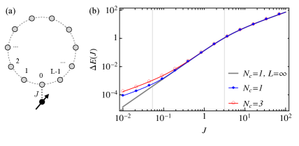
Figure 1: Left: Geometry used in this work. Right: dependence of the energy gain $\Delta E(J)=E_{0}(0)-E_{0}(J)$ on Kondo coupling parameter $J$ for a system with $L=100$ sites with $N_{c}=1$ (blue diamonds and line) and $N_{c}=3$ (red circles and line) conduction electrons. The three regions (explained in text) are clearly visible and separated by vertical lines. The curve with no symbols is the analytical $L=\infty$ result for $N_{c}=1$.

In the original setting for Kondo physics, the coupling $J$ is small compared to the other energy scales such as the bandwidth or Fermi energy. Since the regimes considered here are expected to be relevant to new settings for Kondo physics, we consider $J$ values from $J\ll 1$ to $J\gg 1$ without restriction.

Figure 1 summarizes the behavior of $\Delta{E}(J)$ for small, intermediate and large $J$, for a fixed number of particles ($N_{c}=1$ and $N_{c}=3$) in a large ring with $L\gg 1$. For any finite $L$, there are three clearly different regions of $J$ values, which we will refer to as regions A, B, and C from small to large $J$. Region A (small $J$) is where the Kondo coupling is perturbative. Hence $\Delta{E}(J)$ is linear, with a coefficient that vanishes as $\sim{L}^{-1}$ at large $L$. In region C (large $J$), the Kondo coupling $J$ is so strong that the impurity simply binds one fermion to it in a singlet. As far as the other electrons are concerned, the impurity connected site ($j=0$) is blocked and the ring is cut into an open chain of $(L-1)$ sites. The energy gain is the singlet energy, $\Delta{E}(J)\approx\frac{3}{4}J$. Between these two linear-$J$ regions lies the nonperturbative region B. We will present evidence that there the behavior is $\Delta{E}(J){\sim}J^{2}$ in 1D for fixed small $N_{c}$. This also applies for small densities $n_{c}$ and not too small $J$. For infinite $L$ the region A disappears and region B extends all the way down to infinitesimal $J$; this is seen from the $L=\infty$ curve for $N_{c}=1$ in Figure 1.

I.1 Outline

Using the general orientation to the three $J$-regions provided by these observations on the energy gain $\Delta{E}(J)$, in Section II we will give an overview of the types of situations encountered in this study (fixed number, fixed small density), and explain how these connect to the usual thermodynamic limit and well-known finite density results. In Section III we present renormalization group arguments for the $\Delta{E}(J)$ behavior at finite but small densities. Section IV considers the ultralow density situation of fixed $N_{c}$. In Section IV.1, we detail the case of a single electron ($N_{c}=1$), which is exactly solvable. Results for finite numbers of electrons, $N_{c}>1$, are outlined in Section IV.2. Since our numerical calculations (exact diagonalization) are restricted to smaller $L$ at larger $N_{c}$, the results for $N_{c}=3,5,\ldots$ also provide a description of how the half-filling case is approached, e.g., how spin and charge are more and more decoupled at larger fillings. In Section V, we consider briefly the case of higher dimensions.

II Overview; fixed number versus fixed small densities

Low-density and ultralow-density situations correspond to different orders of limits for system size $L$ and particle number $N_{c}$. Figure 2(a) charts out several different regimes. The usual thermodynamic limit involves both $L\to\infty$ and $N_{c}\to\infty$ while keeping the density $(N_{c}/L)$ fixed. On the $N_{c}$-$L$ plane, this corresponds to going toward large sizes along a finite-slope path, e.g., along one of the shaded paths. Low but finite density corresponds to a steep but finite-slope path. The ultralow-density situation involves fixed $N_{c}$ at arbitrary $L$, including $L\to\infty$, these are vertical lines in Figure 2(a) and do not correspond to the regular thermodynamic limit.

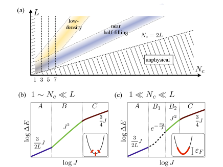
Figure 2: (a) Different regimes on the $N_{c}$-$L$ parameter space: the ultralow-density regime ($N_{c}$ fixed, vertical lines), the low-density regime ($N_{c}/L$ fixed at small value, steep shaded area) and regime near half filling ($N_{c}/L\sim 1$, shaded area with smaller slope). (b,c) schematics showing different $\Delta{E}(J)$ behaviors in different $J$ regions, for the cases of small and large $N_{c}$, respectively. See text for details.

We note that the regimes overlap at smaller $N_{c}$, e.g., the vertical dashed lines cross through the shaded areas indicating the thermodynamic limit. Thus, for finite but large $L$ and finite $N_{c}\ll{L}$, it may be ambiguous to decide whether the physics of the system is best described by low-density results in the thermodynamic limit, or by the ultralow-density physics that does not correspond to the usual thermodynamic limit.

In Figure 2(b,c) we have summarized our results for the energy gain (analogue of the Kondo temperature) in the 1D case; the derivations will appear in later sections. Differences occurring for higher-dimensional baths will be discussed in Sec. V.

Panels 2(b) and 2(c) correspond to $1\sim N_{c}\ll L$ and $1\ll N_{c}\ll L$, respectively. The insets show a rough “band filling” picture of these cases: for small $N_{c}$ one may think of a finite number of single-particle levels of the conduction band being occupied, while for larger $N_{c}$ a picture of small band filling is more appropriate.

In both cases and for finite $L$, there is a finite-size-dominated A region at small $J$ where $\Delta{E}=c_{1}J$, with $c_{1}=\frac{3}{2L}$ in every case except for $N_{c}=1$, where we have $c_{1}=\frac{3}{4L}$. The C region with localized singlet and energy gain $\Delta{E}=\frac{3}{4}J$ is also the same for all cases. These behaviors in A and C regions hold not only for the cases we are considering but even for the half-filling situation.

For the interesting B region, $\Delta{E}(J)$ is nonperturbative. For fixed small $N_{c}$, the behavior is $\Delta{E}\sim{J}^{2}$. For $N_{c}=1$, the exact solution yields $\Delta{E}=\left(\frac{3}{8}J\right)^{2}$. There are no exact solutions for fixed $N_{c}>1$, but we present strong numerical evidence that the energy gain in the B region is identical for $N_{c}=3$, and we conjecture that this applies for all small odd $N_{c}$.

For larger $N_{c}$, shown in Fig. 2(c), the B region can have two types of behavior. If $J$ is small enough that the Kondo energy scale is significantly smaller than the Fermi energy with respect to the band bottom, screening is dominated by electron states around the Fermi points where the dispersion is nearly linear, so that we recover the usual Kondo effect, and one expects a $J$ dependence according to $\Delta{E}(J)\sim e^{-c_{2}/J}$. On the other hand, if $J$ is larger so that the Kondo energy scale is of the order or larger than the Fermi energy, linearization is not possible and the density of states at the bottom of the spectrum has to be taken into account. For the 1D conduction bath, this turns out to lead to $\Delta{E}\sim{J}^{2}$, as described in Section III. We have marked these two regions as B₁ and B₂ in Figure 2(c).

The limit $L\to\infty$ with $N_{c}$ fixed yields the ultralow-density limit announced in the introduction; in this limit only the B (or B₂) and C regions survive. In the low-density limit, with $L\to\infty$ and $N_{c}\to\infty$, there is a B₁ region at small $J$ which connects to the standard (nonperturbative) Kondo setting with $\Delta{E}(J)\sim e^{-c_{2}/J}$. In contrast, the B₂ region occurring for larger $J$ does not have the familiar $e^{-c_{2}/J}$ behavior for the energy gain (in 1D), but nevertheless has nonperturbative behavior.

III Renormalization Group predictions for small finite densities

Results for the low-density case in the thermodynamic limit can be obtained using a perturbative renormalization-group (RG) expansion around the free-moment fixed point of the Kondo model, i.e., a generalizationwithoff ; fv04 of Anderson’s poor man’s scaling.poor We note that the results continue to apply for finite $L$ as long as the bath level spacing is small compared to the Kondo temperature $T_{\rm K}$.

We restrict our attention to the case of a one-dimensional conduction band as in Eq. (1). It is convenient to work in a grand-canonical ensemble, with a chemical potential $\mu$; in the following $\mu$ and all energies will be measured relative to the band bottom. The density of states at small energies is

$$\rho(\omega)=\rho_{0}\left|\frac{\omega}{D}\right|^{r}\Theta(\omega),~{}~{}r=-1/2$$ (2)

with $D=4$ the bandwidth and $\rho_{0}=1/(4\pi)$, such that chemical potential and average filling $n_{c}=N_{c}/L$ are related by

$$n_{c}\propto\mu^{1/2}.$$ (3)

Eqs. (1) and (2) define an unconventional Kondo problem, with non-constant and strongly asymmetric density of states. In the course of the RG, a scattering potential $V$ at the impurity site will be generated which keeps track of the particle–hole asymmetry. For the limiting case of $\mu=0$ the weak-coupling beta functions for the dimensionless running couplings $j=\rho_{0}J$ and $v=\rho_{0}V$ readzawa_asy ; florens07

$$\frac{dj}{d\ln\Lambda}=rj-\frac{j^{2}}{2}+2vj\,,~{}~{}~{}\frac{dv}{d\ln\Lambda}=rv+\frac{3j^{2}}{16}+v^{2}$$ (4)

to second order, with $\Lambda$ being the running UV cutoff, and the initial values $j_{0}=\rho_{0}J$ and $v_{0}=0$ according to Eq. (1).

III.1 Kondo scale

Clearly, for small $j$ and $v$, the first (tree-level) term in the beta function dominates the flow. For $r=-1/2<0$ the initial $j$ grows under RG and diverges at $\Lambda=T_{\rm K}$ withmitchell13

$$T_{\rm K}\propto D\left(\frac{\rho_{0}J}{-r}\right)^{-1/r}=D\left(2{\rho_{0}}J\right)^{2}$$ (5)

As usual, the energy scale $\Lambda=T_{\rm K}$ where $j$ diverges is the estimate for the Kondo energy or temperature scale, expected to be proportional to the energy gain $\Delta{E}$ introduced earlier. This $\mu=0$ result continues to hold for nonzero $\mu$ as long as $T_{\rm K}>\mu$, as in this case the RG flow reaches strong coupling before the deviation from the band edge becomes relevant – this is exactly what defines the region B₂ in Fig. 2.

In the opposite limit $T_{\rm K}\ll\mu$, corresponding to region B₁, the dominant contribution to screening arises from the regime $\Lambda<\mu$ where the density of states can be approximated as constant, $\rho(\mu)=\rho_{0}(\mu/D)^{-1/2}\propto\rho_{0}/n_{c}$.

The standard exponential estimate for the energy scale applies, consequently:

$$T_{\rm K}\propto D\exp\left(-\frac{c_{2}}{J}\right)$$ (6)

with $c_{2}\propto n_{c}/\rho_{0}$.

III.2 Crossovers between the A, B, and C regions

These considerations allow to extract the locations of the crossovers between the various regions. First, the B–C crossover is set by $T_{\rm K}\sim 1$, which implies $\rho_{0}J_{BC}\sim 1$.

Second, the boundary between the B₁ and B₂ regions is defined by $T_{\rm K}\sim\mu$; using Eqs. (3) and (5) this yields $\rho_{0}J_{B12}\sim n_{c}$. Alternatively, we can demand the $T_{\rm K}$ expressions in Eqs. (5) and (6) to match, resulting in $\rho_{0}J_{B12}\ln[1/(\rho_{0}J_{B12})]\sim n_{c}$ which is identical to the first criterion up to logarithmic accuracy. This shows how the region B₁ disappears when passing from the low-density to the ultralow-density limit, $n_{c}\to 0$.

Third, the boundary of the A region can also be found be equating the expressions for $T_{\rm K}$ (or $\Delta E$). Using $\Delta E\propto J/L$ in the A region, this yields for a direct crossover from A to B₂ the relation $\rho_{0}J_{AB2}\sim 1/L$. In contrast, the A–B₁ crossover occurs at $\rho_{0}J_{AB1}\sim N_{c}/(L\ln L)$; this formula is valid only for $N_{c}\gg 1$ and up to logarithmic accuracy.

Taken together, these relations show that $1\sim N_{c}\ll L$ (with $L$ finite) implies a direct crossover from A to B₂ as in Fig. 2(b), whereas for large $N_{c}$ a B₁ region intervenes.

IV Fixed number of conduction electrons (ultralow densities)

In this section we describe systems with a fixed number $N_{c}$ of electrons in the one-dimensional conduction bath. We will restrict to odd numbers of $N_{c}$ so that the total spin is integer and hence can be a singlet. In Section IV.1 we treat analytically the $N_{c}=1$ case and describe the energy gain and spatial profiles. In Section IV.2 we describe $N_{c}>1$, again focusing on the energy gain and spatial profiles. Section IV.3 describes perturbative results for the A (small $J$) region for finite $L$.

IV.1 Exactly solvable case, $N_{c}=1$

Focusing on the solvable case of a single fermion in the bath ($N_{c}=1$), we will derive below the energy gain in B and C regions. We also show that the impurity-bath spin-spin correlator $\chi_{j}=\langle{\vec{S}_{\mathrm{imp}}\cdot\vec{s_{j}}}\rangle$ is locked to the density profile $n_{j}=\sum_{\sigma}\langle{c_{j\sigma}^{\dagger}c_{j\sigma}}\rangle$, through the relation $\chi_{j}=-\frac{3}{4}n_{j}$.

The three $J$-regions have simple spatial interpretations in terms of the density profile of the single electron. In an infinite chain, in the ground state, the fermion is localized around the impurity-coupled site ($i=0$) with localization length $\xi$. ($\xi$ decreases with increasing $J$.) At large $J$ (region C), the itinerant fermion is almost completely localized at site 0 ($\xi\lesssim 1$). At smaller $J$, the itinerant fermion is spread over multiple sites $\xi>1$ (region B). In an infinite system, this region would extend to arbitrarily small $J$. However, for any finite size $L$, there is a boundary-sensitive small-$J$ region (region A) where the fermion cloud extends over the whole system ($\xi\gtrsim{L}$).

IV.1.1 Analytic solution for energy gain

To examine the ground state, we restrict to the singlet sector. Within this sector, the states can be written in the basis of single-particle momentum eigenstates

$$\left|{k}\right.\rangle=\frac{1}{L\sqrt{2}}\sum_{j}e^{-ikj}\Big{(}\left|{\uparrow;j\downarrow}\right.\rangle-\left|{\downarrow;j\uparrow}\right.\rangle\Big{)}\,.$$ (7)

The $\left|{S;js}\right.\rangle$ notation refer to the impurity spin $S$ and the electron position $j$ and spin $s$. Within the singlet sector the Kondo coupling serves as a local potential on the site $j=0$, of strength $-\frac{3}{4}J$, i.e., this sector is described by a single-particle problem in a resonant level model:

$$H~{}=~{}-2\sum_{k}\left|{k}\right.\rangle\cos k\langle\left.{k}\right|-\frac{3}{4}\frac{J}{L}\sum_{k,k^{\prime}}\left|{k}\right.\rangle\langle\left.{k^{\prime}}\right|$$ (8)

The components $\psi_{k}$ of an eigenstate $\left|{\psi}\right.\rangle=\sum_{k}\psi_{k}\left|{k}\right.\rangle$ with energy $E$ obey the relation

$$\left(-2\cos k-E\right)\psi_{k} = \frac{3}{4}\frac{J}{L}\sum_{k^{\prime}}\psi_{k^{\prime}}$$ (9)

Summing over $k$ one gets closed equations for $E$ and for $\psi_{k}$

$$1 = \frac{3}{4}\frac{J}{L}\sum_{k}\left(-2\cos k-E\right)^{-1}$$ (10)

$$\psi_{k} = \frac{1}{\mathcal{N}}\left(-2\cos k-E\right)^{-1}$$ (11)

where $\mathcal{N}$ is a normalization constant. This gives all the singlet eigenstates at finite $L$. For $L\to\infty$ the continuum version of Eq. (10) gives the ground-state energy, because the rest of the states are part of a continuum in $E\in\left[-2,2\right]$. The ground state energy $E_{0}$ thus satisfies $\frac{4}{3J}=-\int\frac{dk/(2\pi)}{2\cos k+E_{0}}$, leading to $E_{0}=-\sqrt{\left(\tfrac{3}{4}J\right)^{2}+4}$, so that the energy gain, $\Delta E=-2-E_{0}$, is

$$\Delta{E}=-2~{}+~{}\sqrt{\left(\tfrac{3}{4}J\right)^{2}+4}~{}\approx~{}\begin{cases}\frac{9}{64}J^{2}&J\ll 1\\ \frac{3}{4}J&J\gg 1\end{cases}$$ (12)

This is the solid curve in Figure 1. For finite $L$, the $\frac{9}{64}J^{2}$ behavior gets cut off at smaller $J$ and is replaced by the A region, $\Delta{E}\approx\frac{3}{2}J$. This can be numerically extracted from Eq. (10) or can be calculated perturbatively (subsection IV.3).

IV.1.2 Real-space profiles; density and spin correlator

The density is

$$n_{j} = \sum_{s}\left\langle c_{j,s}^{\dagger}c_{j,s}\right\rangle=\left|\psi_{j}\right|^{2}=\left|\frac{1}{\sqrt{L}}\sum_{k}e^{-ikj}\psi_{k}\right|^{2}$$ (13)

with $\psi_{k}$ given by Eq. (11). The impurity-bath spin-spin correlator is

$$\chi_{j} = \left\langle\vec{S}_{\mathrm{imp}}\cdot\vec{s}_{j}\right\rangle=-\frac{3}{4}\left|\psi_{j}\right|^{2}=-\frac{3}{4}n_{j}\,,$$ (14)

showing that the two quantities are locked to each other in the $N_{c}=1$ case. In the $L\to\infty$ limit, one obtains $n_{j}\propto e^{-|j|/\xi}$, with

$$\xi^{-1}=-\ln\left[\sqrt{\left(\tfrac{3}{8}J\right)^{2}+1}-\tfrac{3}{8}J\right].$$ (15)

For finite $L$, the density (and $\chi_{j}$) profile is exponentially localized around the impurity site in the B and C regions, but is modified by the boundary in the A region, as shown in Figure 3(a-c). Figure 3(d) compares the expression (15) with the length scale $\tilde{\xi}$ obtained from an exponential fit $f_{1}(x)=A_{1}\exp[-x/\tilde{\xi}]$ in the B and C regions ($J\gtrsim 1$) for a $L=100$ system. In the A region, we find that the real-space profile is well-described by the corrected form $f_{2}(x)=A_{2}\exp[-x/\tilde{\xi}+x^{2}/(\tilde{\xi}L)]$; Figure 3(d) also compares $\tilde{\xi}$ obtained with this fit in the A region.

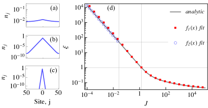
Figure 3: Ground state for single bath electron ($N_{c}=1$), $L=100$. (a-c) Density profiles in A, B, C regions: $J=0.02$; $J=0.5$; $J=5$. (d) The localization length $\xi$. Black solid line is analytic large-$L$ expression (15). Filled dots are obtained by fitting function $f_{1}(x)$ (see text) to $(\frac{L}{2}-1)$ sites around the impurity. Open dots in the A region are obtained by fitting $f_{2}(x)$.

IV.1.3 Entanglement entropy profile

We will now characterize the spatial structure of the system using block-block entanglement entropy, $S(J,r)=-\text{Tr}\left[\rho_{r}\ln\rho_{r}\right]$, where $\rho_{r}$ is the reduced density matrix of a block containing the impurity spin and the $(2r-1)$ sites centered around the impurity-coupled site. This is analogous to studies in finite-density impurity systems where block entanglement entropies have been used to describe the real-space impurity screening cloud. SorensenLaflorencieAffleck ; SaleurVasseur_PRB13 ; GhoshRibeiroHaque_2013

Figure 4(a) shows the typical behaviors of the entanglement entropy as a function of block size, for $J$ values in the A, B, C regions. In the C region, $S(J,r)$ is nearly zero for all $r>1$, since the electron is localized at the impurity-coupled site. In the B region, there is structure indicative of the localization length $\xi(J)$. The A region curve is the entanglement entropy of a uniform system; the lack of left-right symmetry is due to the block containing the impurity spin and therefore being inequivalent to its complement when containing half the lattice sites.

In panel (b) the entanglement entropy is shown for block size $r=1$, i.e., the block contains only the impurity and the site $j=0$. In the extreme C region the cloud is completely localized on this site, so that the rest of the system is decoupled, $S_{J\to\infty}(J,r)\to 0$. In the extreme A region the density is uniform, so that the entanglement entropy has constant $L$-dependent value. Constructing the density matrix explicitly, we obtain for this uniform case

$$S(J=0,r=1)=\frac{L-1}{L}\log\left(\frac{2L}{L-1}\right)+\frac{1}{L}\log\left(L\right).$$ (16)

In the B and C regions, the electronic cloud decays exponentially $n_{j}\propto e^{-j/\xi(J)}$ where $\xi(J)$ is given in Eq. (15). Explicit calculation gives

$$S_{\mathrm{Expon}}(J,r=1)~{}=~{}-2M_{1}\log{M_{1}}~{}-~{}M_{2}\log{M_{2}}\,,$$ (17)

with $M_{1}(J)=\left[1+e^{1/\xi(J)}\right]^{-1}$ and $M_{2}(J)=\tanh\left(\frac{1}{2\xi(J)}\right)$. Figure 4(b) shows the above expressions together with the exact numerical $S(J,1)$ for $L=100$. The exact curve moves from $S(0,1)$ to $S_{\mathrm{Expon}}(J,1)$ as $J$ is increased from the A to the B region; the two curves cross near $J=\frac{16}{3L}$, which is the boundary between A and B regions at large $L$ as obtained from the condition $\xi(J)=L/2$.

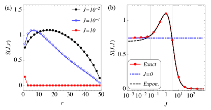
Figure 4: Entanglement entropy $S(J,r)$ for $N_{c}=1$, $L=100$, between a block containing the impurity and the $(2r+1)$ bath sites around it, and the rest of the system. (a) $S(J,r)$ against block size $r$, for one $J$ value each in the A, B, C regions. (b) $S(J,1)$ against $J$. Exact numerical curve crosses over from the constant $S(0,1)$ value to the curve $S_{\mathrm{Expon}}(J,1)$ calculated assuming exponentially localized electron, Eq. (16) to Eq. (17). Vertical lines demarcate A, B, C regions.

IV.2 Few mobile electrons; $N_{c}>1$

We now look at the energy gain and the real-space profiles for a few fermions ($N_{c}$ odd and $>1$) in a 1D bath. As we shall show, a general feature is that, for $L\to\infty$, the $N_{c}>1$ systems behave in some ways similar to the $N_{c}=1$ system. We will see this both in the energy gain and in the real-space profiles. Intuitively, the reason is that for large $L$ the ground state involves one of the bath fermions localized around the impurity while the other fermions spread out with vanishing density and therefore negligible effect. Thus the physics of the impurity interacting with a single fermion is dominant, so that one recovers signatures of the energy gain $\Delta{E}$ and localization length $\xi$ derived in Section IV.1.

IV.2.1 Energy gain

Unlike the $N_{c}=1$ case, it is not possible to obtain an analytical expression or simple equation for $\Delta{E}$. However, numerical calculation (Figure 1) shows that there are three $J$ regions with the same characteristics. For large $J$ (C region) the energy gain is the singlet energy $\Delta{E}\approx\frac{3}{4}J$. At small $J$ (A region) the energy gain is perturbative and $L$-dependent, $\Delta{E}\sim\frac{3}{4L}J$ for any $N_{c}>1$ (Section IV.3). This is half the energy gain for $N_{c}=1$ in the A region.

The intermediate $J$ region (B region) is more tricky to characterize; it is not straightforward to infer the $J$-dependence in the B region by looking only at the numerical $\Delta{E}(J)$ with available sizes. Analyzing instead the second derivative $\partial_{JJ}\Delta E(J)$, we provide numerical evidence that in the $L\to\infty$ limit the $\Delta{E}(J)$ curve for $N_{c}>1$ coincides with the $\Delta{E}(J)$ curve calculated for $N_{c}=1$. This implies that the B region is described by $\Delta{E}\sim\frac{9}{64}J^{2}$ also for $N_{c}>1$.

Figure 5(a) shows the second derivative for $N_{c}=3$, for system sizes from $L=10$ to $L=100$. Clearly, $\partial_{JJ}\Delta E(J)$ approaches the $L\to\infty$ solution of the single-electron ($N_{c}=1$) case. In Figure 5(b) we show the difference between the maximum value of $\partial_{JJ}\Delta E(J)$ of the finite-size $N_{c}=3$ data, from the exact $N_{c}=1$ solution. The difference decreases with $L$, apparently with a super-linear power law. This provides relatively strong evidence that, in the limit $L\gg\infty$, the B region for $N_{c}=3$ has identical $\Delta{E}(J)$ behavior as for the exactly solved $N_{c}=1$ case.

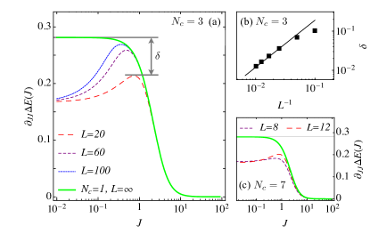
Figure 5: (a) Second derivative of the energy gain $\partial_{JJ}\Delta E(J)$ for $N_{c}=3$ mobile electrons and different $L$. Thick solid line shows the exact $\partial_{JJ}\Delta E(J)$ for $N_{c}=1$, $L\to\infty$, Eq. (12). With increasing $L$, the 3-electron curves clearly approach the exact 1-electron curve. (b) Difference between maximum of the $N_{c}=3$ curves $\partial_{JJ}\Delta E(J)$ and the maximum of the $N_{c}=1$ curve, against $L$. (c) Similar data as (a), but for $N_{c}=7$ electrons.

For larger $N_{c}$, it is difficult to use large enough $L$ for a proper finite-size scaling analysis. However, Figure 5(c) shows the second derivative $\partial_{JJ}\Delta E(J)$ for $N_{c}=7$ conduction electrons in a $L=8$ bath and in a $L=12$ bath. The features of these curves, and the way in which they approach the analytic $N_{c}=1$ curve with increasing $L$, are very similar to the $N_{c}=3$ case. This leads us to suggest that for any fixed odd $N_{c}\geq 3$, the B₂ region is described by $\Delta{E}\sim\frac{9}{64}J^{2}$. As discussed in Section III, for $N_{c}\gg 1$ there will be an additional B₁ region at small $J$ with exponential behavior of $\Delta E$; this is not captured by our finite-size numerics.

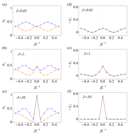
Figure 6: Real space profiles in an $L=12$ bath: (a-c) electronic density $n_{j}$; (d-f) impurity-bulk spin susceptibility $\chi_{j}$. Each panel shows data for $N_{c}=3$ (filled orange circles) and $N_{c}=5$ (empty blue circles).

IV.2.2 Real space profiles; density and spin correlator

Figure 6 plots the spatial dependence of the total electronic density $n_{j}$ and the impurity-bulk spin correlator $\chi_{j}$ for $N_{c}=3$ and $N_{c}=5$, with $L=12$ sites.

For $J\ll{1}$, the densities are primarily determined by the bath. The single-particle spectrum of the bath includes two degenerate states at momentum $k=0$, and four degenerate states each at momenta $k=\pm\frac{2\pi}{L}n$. Thus the cases of $N_{c}=4n-1$ and $N_{c}=4n+1$ are closely linked, corresponding to having one or three states filled among the highest 4-fold degenerate set. This explains why the density profiles for $N_{c}=3$ and $N_{c}=5$ are closely linked. The density profiles for $N_{c}=7$ and $N_{c}=9$ form a similar pair. More strikingly, the correlator $\chi_{j}$ are identical for $N_{c}=4n-1$ and $N_{c}=4n+1$ in the $J\ll{1}$ limit. These features in the perturbative $J\ll 1$ region will be explained in more detail in Section IV.3.

Similar arguments can be made in the large-$J$ limit, where one particle is bound to the impurity and the remaining $(N_{c}-1)$ fermions can be treated as free fermions in an open-boundary $(L-1)$-site chain. Again, the $N_{c}=3$ and $N_{c}=5$ density profiles are closely linked, and the spin correlators are nearly identical. Surprisingly, we find $\chi_{j}$ for $N_{c}=4n-1$ and $N_{c}=4n+1$ to be nearly identical even for intermediate $J$ (Figure 6 middle row), where we cannot use free-fermion ideas to explain this feature.

For large $L$, the real-space behaviors for finite $N_{c}>1$ is governed by the single-electron localization length. In Figure 6 we illustrate this through the spin correlator $\chi_{j}$. We extract the length scale of localization around the impurity by fitting $\left|\chi_{j}\right|$ to $f_{1}(x)=A_{1}\exp[-x/\xi_{\chi}]$ in the B and C regions, using $\chi_{j}$ on only three sites near the impurity to avoid complications such as sign changes of $\chi_{j}$ at larger $j$. For small $J$, it is necessary to incorporate the boundary with the modified exponential $f_{2}(x)=A_{2}\exp[-x/\tilde{\xi}+x^{2}/(\tilde{\xi}L)]$, as in the 1-electron case. In addition, from Figure 6 (top row) it is clear that an overall $2k_{F}$ oscillation is important at small $J$. Therefore for small $J$ a fit with $f_{2}(x)\cos^{2}(2\pi{x}/L)$ is used to extract the length scale $\xi_{\chi}$. In this case about 35% of the sites are used for the fit.

Figure 7(a) compares the length scale $\xi_{\chi}$ extracted numerically from the 3-electron $\chi_{j}$, with the 1-electron result $\xi^{\mathrm{1el}}$ from Eq. (15). The close match indicates that the localization is governed by the $N_{c}=1$ length scale. Figure 7(b) shows that this match gets better with increasing $L$, by plotting the relative difference, $\eta(\xi_{\chi})=\left|\xi_{\chi}-\xi^{\mathrm{1el}}\right|/\xi_{\mathrm{1el}}$, between the 1-electron length scale and the 3-electron length scale obtained from a $f_{1}(x)$ fit. (The $f_{1}$ fit is not expected to be reasonable at small $J$.) Figure 7(c) shows that $f_{2}(x)\cos^{2}(2\pi{x}/L)$ is a meaningful description for moderate distances from the impurity.

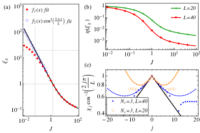
Figure 7: (a) Decay length scale of $\chi_{j}$ close to the impurity, for $L=40$, $N_{c}=3$. Length scale $\xi_{\chi}$ obtained from $f_{1}(x)$ fit (red dots), and from $f_{2}(x)\cos^{2}(2\pi{x}/L)$ fit (open blue squares) are shown. Localization length for $N_{c}=1$ is given by solid line. (b) The relative difference between $N_{c}=3$ and $N_{c}=1$ electron exponents $\eta(\xi_{\chi})$ is shown for $L=40$ and $L=20$. Here $\xi_{\chi}$ is obtained by fitting with $f_{1}$. (c) For $J=0.1$, the exact numerical $\chi_{j}$ data are shown together with best fits with $f_{2}(x)\cos^{2}(2\pi{x}/L)$. The oscillatory factor is divided out. Exact data are shown as open orange circles ($L=20$) and filled blue circles ($L=40$); fits are shown with orange dashed line and blue dotted lines. Black solid line shows $\chi_{j}$ for $N_{c}=1$, $L=40$.

Figure 8 shows how the density $n_{j}$ and the spin structure $\chi_{j}$ gradually decouple as half-filling is approached. We have shown (Section IV.1) that the $n_{j}$ and $\chi_{j}$ profiles are locked together (proportional to each other) for $N_{c}=1$. Figure 8 shows $n_{j}$ and $\chi_{j}$ to be very similar for $L{\gg}N_{c}=3$, while at half filling with $N_{c}=L=9$ they bear little resemblance to each other. In the half-filled situation at large sizes and small $J$, $n_{j}$ is essentially constant, while the spatial profile of $\chi_{j}$ characterizes the so-called Kondo cloud. Goth_Assaad ; ishii ; BarzykinAffleck_PRB98 ; BordaGarstKroha_PRB09 ; Borda_PRB07 ; Holzner-etal_PRB09

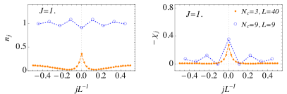
Figure 8: Spin-charge decoupling upon approaching half filling. A $N_{c}{\ll}L$ case and a $N_{c}=L$ case are shown.

IV.3 Analytic expressions for the A region, $J\ll{1}$

For the A region, one can perturbatively calculate the energy gain $\Delta{E}(J)$. This gives the coefficient of the linear ${\sim}L^{-1}J$ dependence in this region. Also, by examining the perturbative expressions for $n_{j}$ and $\chi_{j}$ profiles, one can expain the close relationship (Figure 6) between profiles of $N_{c}=4n\pm 1$ pairs, where $n$ is an integer.

IV.3.1 Perturbative calculation for energy gain

The ground state of the hopping part of the Hamiltonian, is degenerate. The degeneracy is 2-fold for $N_{c}=1$ and 4-fold for $N_{c}\geq 3$.

We first consider $N_{c}\geq 3$. For $N_{c}=4n+1$, the four degenerate states for $J=0$ are

$$\left|{\Psi_{1}}\right.\rangle= \left|{\downarrow}\right.\rangle\otimes\left|{0\uparrow,0\downarrow,\ldots,\mathrm{k_{F}}\uparrow}\right.\rangle,$$ (18)

$$\left|{\Psi_{2}}\right.\rangle= \left|{\downarrow}\right.\rangle\otimes\left|{0\uparrow,0\downarrow,\ldots,-\mathrm{k_{F}}\uparrow}\right.\rangle,$$

$$\left|{\Psi_{3}}\right.\rangle= \left|{\uparrow}\right.\rangle\otimes\left|{0\uparrow,0\downarrow,\ldots,\mathrm{k_{F}}\downarrow}\right.\rangle,$$

$$\left|{\Psi_{4}}\right.\rangle= \left|{\uparrow}\right.\rangle\otimes\left|{0\uparrow,0\downarrow,\ldots,-\mathrm{k_{F}}\downarrow}\right.\rangle,$$

where the states are written as products of the impurity spin state and the bath state. The $N_{c}$-particle bath states are written by specifying the single-particle momentum and spin of the particles; the states above are obtained by filling up the single-particle states up to the Fermi momentum. There are four ground states because there are four single-particle states with moemntum $\pm{k_{F}}$, and the last bath electron can fill any one of them. For $N_{c}=4n-1$, the last bath electron can keep any one of the last four states empty, so that there are also 4 ground states.

The Kondo-coupling part of the Hamiltonian, $H_{K}$, is now the perturbation. The matrix elements $H_{ij}=H_{ji}=\langle\left.{\Psi_{i}}\right|H_{K}\left|{\Psi_{j}}\right.\rangle$ of the degeneracy matrix are found to be

$$H_{ii}=H_{12}=H_{34}= -\frac{J}{4L}\,,$$ (19)

$$H_{31}=H_{41}=H_{32}=H_{42}= \frac{J}{2L}\,.$$ (20)

The smallest eigenvalue of the $H_{ij}$ matrix gives the most negative energy correction, and hence the ground-state energy gain at first order is

$$\Delta E=\frac{3}{2}\frac{J}{L}\qquad\mathrm{for}\quad N_{c}\geq 3.$$ (21)

The corresponding eigenstate is

$$\left|{\Psi_{g}}\right.\rangle=\frac{1}{2}\left(\left|{\Psi_{1}}\right.\rangle+\left|{\Psi_{2}}\right.\rangle-\left|{\Psi_{3}}\right.\rangle-\left|{\Psi_{4}}\right.\rangle\right).$$ (22)

For $N_{c}=1$, the ground state is 2-fold degenerate: the states can be taken as $\left|{\Psi_{1}}\right.\rangle$ and $\left|{\Psi_{3}}\right.\rangle$, using the notation introduced above, with $\mathrm{k_{F}}=0$. Matrix elements are the same: $H_{11}=H_{33}=-\frac{J}{4L}$, $H_{31}=\frac{J}{2L}$. The smallest eigenvalue of the degeneracy matrix is

$$\Delta E=\frac{3}{4}\frac{J}{L}\qquad\mathrm{for}\quad N_{c}=1.$$ (23)

IV.3.2 Density and spin correlation function at $J\rightarrow 0^{+}$

Using the ground state (22) from perturbation theory we also calculate the electron density $n_{j}$ and the spin-spin correlation function $\chi_{j}$. After expressing the operators $\hat{n}_{j}=\sum_{s}c^{\dagger}_{j,s}c_{j,s}$ and $\vec{S}_{\mathrm{imp}}\cdot\vec{s_{j}}=\vec{S}_{\mathrm{imp}}\cdot\sum_{s,s^{\prime}}c_{j,s}^{\dagger}\vec{\sigma}_{ss^{\prime}}c_{j,s^{\prime}}$ in momentum basis, the expectation values in state (22) are found to be

$$n_{j}~{}=~{}\frac{N_{c}}{L}-\frac{1}{L}\sin\left(\tfrac{\pi}{2}N_{c}\right)\cos\left(2\mathrm{k_{F}}j\right).$$ (24)

and

$$\chi_{j}=-\frac{3}{4L}\left(1+\cos(2\mathrm{k_{F}}j)\right)$$ (25)

The factor $\sin\left(\tfrac{\pi}{2}N_{c}\right)$ used above has values $\pm 1$ for $N_{c}=4n\pm 1$; Eq. (24) explains Figure 6(a). Eq, (25) shows that the impurity-bath spin-spin correlator profiles for $N_{c}=4n\pm 1$ cases (same $k_{F}$) are identical at small $J$, Figure 6(d).

V Higher-dimensional baths

While our main focus in this paper has been on 1D conduction baths, we will comment now on higher-dimensional baths. Little changes occur in the regions A and C: Region C is dominated by local singlet formation, such that $\Delta E\approx\frac{3}{4}J$ continues to hold. Region A remains perturbative, with $\Delta E\propto\frac{J}{L}$ and a prefactor depending on $N_{c}$ and the lattice geometry.

In contrast, changes are expected in the nonperturbative B region, as the phase space (or density of states) near the band bottom depends on the number of space dimensions. Therefore, the region-B expression for $\Delta{E}$ in the ultralow-density case (Section IV) as well as the region-B₂ expression for $T_{\rm K}$ in the low-density case (Section III) are specific to 1D and are different in higher dimensions.

As an example, let us consider the ultralow-density case with a single electron $N_{c}=1$ in an infinite 2D square-lattice bath. The integral expression for the ground state energy $E_{0}$ in Section IV.1 is modified to

$$\frac{4}{3J}=-\int\frac{dk_{x}dk_{y}/(2\pi)^{2}}{2\cos\left(k_{x}\right)+2\cos\left(k_{y}\right)+E_{0}}\,.$$ (26)

Unlike the 1D case, this cannot be solved analytically for $E_{0}(J)$. However, for small $J$, the energy gain $\Delta{E}=-4-E_{0}$ is found to have the behavior

$$\lim_{J\to 0}\Delta{E}=32e^{-16\pi/3J}\,.$$ (27)

Our results in 1D suggest that the energy gain might have the same behavior for any finite odd $N_{c}>1$ in an infinite lattice; however, it is difficult to check this conjecture numerically in 2D.

For the low-density (finite $N_{c}/L$) case, the calculation of Section III is modified in larger dimensions. For $d=2$ the density of states now follows Eq. (2) with exponent $r=0$, such that the tree-level terms in Eq. (4) are absent. Then, the one-loop result for $T_{\rm K}$ at $\mu=0$ iszawa_asy

$$T_{\rm K}\propto D\exp\left(-\frac{3}{4\rho_{0}J}\right)$$ (28)

where the factor $3/4$ is a result of the particle–hole asymmetry; this result continues to hold in region B₂. In contrast, region B₁ yields the standard formula

$$T_{\rm K}\propto D\exp\left(-\frac{1}{\rho_{0}J}\right).$$ (29)

The crossover between the two regions remains defined by $T_{\rm K}\sim\mu$ which now gives an estimate for the boundary as $\rho_{0}J_{B12}\sim-1/\ln n_{c}$.

The behavior in $d=3$ is more intriguing: Here, the density of states is given by Eq. (2) with exponent $r=1/2$. As a result of the vanishing $\rho(\omega=0)$ there will be no Kondo screening for $\mu=0$ and small $J$.withoff Instead, a quantum phase transition will occur at $\mu=0$ between an unscreened and a screened phase upon increasing $J$.grand_note This quantum phase transition will be smeared for $\mu>0$, in a manner similar to that discussed for doped graphene in Ref. epl, . From $\rho(\mu)\propto\mu^{1/2}$ and $n_{c}\propto\mu^{3/2}$ we can estimate $T_{\rm K}$ for small $J$ from the standard Kondo formula, resulting in

$$T_{\rm K}\propto D\exp\left(-\frac{c_{3}}{J}\right)$$ (30)

where $c_{3}\propto 1/(\rho_{0}n_{c}^{1/3})$. This estimate applies to both B₁ and B₂ regions, however, with different $c_{3}$ prefactors in the exponential, similar to Eqs. (28,29). A more detailed analysis of the crossovers in the $d=3$ case will be given elsewhere.

VI Summary and Conclusions

In this work we have presented a study of Kondo physics at very low bath densities, so that particle-hole symmetry is strongly violated. We have distinguished between two ways of taking the infinite bath limit, one of them corresponding to the usual thermodynamic limit at low densities, and the other with fixed particle number, which we call the ultralow-density limit. To the best of our knowledge, these regimes have not been studied in depth in the literature (see however Refs. Zaanen_PRB92, ; Shchadilova_Ribeiro_arXiv13, ). Either of these two situations may conceivably be realized in the near future in novel experimental conditions.

In both low-density and ultralow-density cases, there are three clearly distinguishable regions of coupling: a large $J$ region where one of the bath electrons is strongly localized forms a localized singlet with the impurity, an intermediate non-perturbative region where the singlet formation is not sharply localized, and (for finite-sized baths) a small-$J$ perturbative region. In the low-density case, the intermediate region is farther demarcated into $J$ values for which the physics is dominated by the Fermi surface or by the band edge. Our focus has mostly been specific to 1D baths, but we have provided some considerations on higher-dimensional baths in the penultimate section.

The present work opens up several open questions and directions of study. Perhaps most prominently, it motivates a full analysis of (ultra)low-density situations in higher dimensions, and also for various lattice geometries. Our brief treatment of 2D shows, for example, that the intermediate-$J$ energy gain is described by different nonperturbative behaviors in 1D and 2D. The role of bath dimensionality or geometry in determining density profiles ($n_{j}$ and $\chi_{j}$) is also currently unclear. Other questions include the influence of interactions in the bath — this has been addressed for the usual finite-density situation, Kondo-in-correlated-els_various ; Kondo-in-correlated_1D but the effects will conceivably be different in the (ultra)low-density cases.

- (1) J. Kondo, Prog. Theor. Phys. 32, 37 (1964).
- (2) A. C. Hewson, The Kondo Problem to Heavy Fermions (Cambridge University Press, New York, 1993).
- (3) W. B. Thimm, J. Kroha, and J. von Delft, Phys. Rev. Lett. 82, 2143 (1999).
- (4) R. K. Kaul, D. Ullmo, S. Chandrasekharan, H. U. Baranger, Europhys. Lett. 71, 973 (2005).
- (5) R. K. Kaul, G. Zaránd, S. Chandrasekharan, D. Ullmo, and H. U. Baranger. Phys. Rev. Lett. 96, 176802 (2006).
- (6) T. Hand, J. Kroha, and H. Monien, Phys. Rev. Lett. 97, 136604 (2006).
- (7) R. K. Kaul, D. Ullmo, G. Zaránd, S. Chandrasekharan, and H. U. Baranger, Phys. Rev. B 80, 035318 (2009).
- (8) C. H. Booth, M. D. Walter, M. Daniel, W. W. Lukens, and R. A. Andersen. Phys. Rev. Lett. 95, 267202 (2005).
- (9) J. Zittartz and E. Müller-Hartmann, Z. Phys. 232, 11 (1970).
- (10) K. Satori, H. Shiba, O. Sakai, and Y. Shimizu, J. Phys. Soc. Jpn. 61, 3239 (1992).
- (11) D. Withoff and E. Fradkin, Phys. Rev. Lett. 64, 1835 (1990).
- (12) C. R. Cassanello and E. Fradkin, Phys. Rev. B 53, 15079 (1996) and 56, 11246 (1997).
- (13) K. Sengupta and G. Baskaran, Phys. Rev. B 77, 045417 (2008).
- (14) T. O. Wehling, A. V. Balatsky, M. I. Katsnelson, A. I. Lichtenstein, and A. Rosch, Phys. Rev. B 81, 115427 (2010).
- (15) L. Dell’Anna, J. Stat. Mech., P01007 (2010).
- (16) M. Vojta, L. Fritz, and R. Bulla, EPL 90, 27006 (2010).
- (17) B. Uchoa, T. G. Rappoport, and A. H. Castro Neto, Phys. Rev. Lett. 106, 016801 (2011); ibid. 106, 159901(E) (2011).
- (18) L. Fritz and M. Vojta, Rep. Prog. Phys. 76, 032501 (2013).
- (19) J. Bauer, C. Salomon, and E. Demler, Phys. Rev. Lett. 111, 215304 (2013).
- (20) A. Holzner, I.P. McCulloch, U. Schollwöck, J. von Delft, and F. Heidrich-Meisner, Phys. Rev. B 80, 205114 (2009).
- (21) L. Borda, Phys. Rev. B 75, 041307(R) (2007).
- (22) L. Borda, M. Garst, and J. Kroha, Phys. Rev. B 79, 100408(R) (2009).
- (23) F. Goth, D. J. Luitz, and F. F. Assaad, arXiv:1302.0856
- (24) V. Barzykin and I. Affleck, Phys. Rev. B 57, 432 (1998).
- (25) H. Ishii, J. Low Temp. Phys. 32, 457 (1978).
- (26) I. Affleck, L. Borda, and H. Saleur, Phys. Rev. B 77, 180404(R) (2008).
- (27) C. A. Büsser, G. B. Martins, L. Costa Ribeiro, E. Vernek, E. V. Anda, and E. Dagotto, Phys. Rev. B 81, 045111 (2010).
- (28) J. Simonin, arXiv:0708.3604.
- (29) A. K. Mitchell, M. Becker, and R. Bulla, Phys. Rev. B 84, 115120 (2011).
- (30) G. Bergmann, Phys. Rev. B 77, 104401 (2008).
- (31) I. Affleck and P. Simon, Phys. Rev. Lett. 86, 2854 (2001).
- (32) P. Simon and I. Affleck, Phys. Rev. B 64, 085308 (2001).
- (33) P. Simon and I. Affleck, Phys. Rev. Lett. 89, 206602 (2002).
- (34) P. Simon and I. Affleck, Phys. Rev. B 68, 115304 (2003).
- (35) E. S. Sørensen, M. S. Chang, N. Laflorencie, and I. Affleck, J. Stat. Mech.: Theory Exp. (2007) P08003; (2007) L01001.
- (36) A. Bayat, P. Sodano, and S. Bose, Phys. Rev. B 81, 064429 (2010).
- (37) R. G. Pereira, N. Laflorencie, I. Affleck, and B. I. Halperin, PRB (2008).
- (38) E. S. Sørensen and I. Affleck, Phys. Rev. B 53, 9153 (1996).
- (39) L. Fritz and M. Vojta, Phys. Rev. B 70, 214427 (2004).
- (40) P. W. Anderson, J. Phys. C 3, 2436 (1970).
- (41) O. Ujsaghy, K. Vladar, G. Zarand, and A. Zawadowski, J. Low Temp. Phys. 126, 1221 (2002).
- (42) S. Florens, L. Fritz, and M. Vojta, Phys. Rev. B 75, 224420 (2007).
- (43) A. K. Mitchell, M. Vojta, R. Bulla, and L. Fritz, Phys. Rev. B 88, 195119 (2013).
- (44) S. Ghosh, P. Ribeiro, and M. Haque, arXiv:1309.0027.
- (45) H. Saleur, P. Schmitteckert, and R. Vasseur, Phys. Rev. B 88, 085413 (2013).
- (46) At it is important to work in a grand-canonical ensemble: For large there will be one conduction electron in the system which is bound to the impurity.
- (47) O. Gunnarsson and J. Zaanen, Phys. Rev. B 46, 15019 (1992).
- (48) Y. E. Shchadilova, P. Ribeiro, and M. Haque, arXiv:1303.4103.
- (49) G. Khaliullin and P. Fulde, Phys. Rev. B 52, 9514 (1995). T. Schork, Phys. Rev. B 53, 5626 (1996). W. Hofstetter, R. Bulla, and D. Vollhardt, Phys. Rev. Lett. 84, 4417 (2000). M. Neef, S. Tornow, V. Zevin, and G. Zwicknagl, Phys. Rev. B 68, 035114 (2003). S. Nishimoto and P. Fulde, Phys. Rev. B 76, 035112 (2007).
- (50) D.-H. Lee and J. Toner, Phys. Rev. Lett. 69, 3378 (1992). A. Furusaki and N. Nagaosa, Phys. Rev. Lett. 72, 892 (1994). A. Schiller and K. Ingersent, Phys. Rev. B 51, 4676 (1995). P. Fröjdh and H. Johannesson, Phys. Rev. Lett. 75, 300 (1995); Phys. Rev. B 53, 3211 (1996). R. Egger and A. Komnik, Phys. Rev. B 57, 10620 (1998). X. Wang, Mod. Phys. Lett. B 12, 667 (1998). K. Le Hur, Phys. Rev. B 59, R11637 (1999).