Active Microrheology of Driven Granular Particles

Abstract

When pulling a particle in a driven granular fluid with constant force $F_{ex}$, the probe particle approaches a steady-state average velocity $v$. This velocity and the corresponding friction coefficient of the probe $\zeta=F_{ex}/v$ are obtained within a schematic model of mode-coupling theory and compared to results from event-driven simulations. For small and moderate drag forces, the model describes the simulation results successfully for both the linear as well as the nonlinear region: The linear response regime (constant friction) for small drag forces is followed by shear thinning (decreasing friction) for moderate forces. For large forces, the model demonstrates a subsequent increasing friction in qualitative agreement with the data. The square-root increase of the friction with force found in [Fiege et al., Granular Matter $\bm{14}$, 247 (2012)] is explained by a simple kinetic theory.

I Introduction

Active microrheology (AM) studies the mechanical response of a many-particle system on the microscopic level by pulling individual particles through the system either with constant force or at constant velocity Squires and Mason (2010). While in passive microrheology only the linear response can be probed, AM can also be applied to explore the non-linear response by imposing large drag forces. An external force $F_{ex}$ can be imposed by magnetic Habdas et al. (2004) or optical tweezers Meyer et al. (2006) to a probe particle embedded in a soft material and then the responding steady-state velocity $\big{\langle}v\big{\rangle}$ is measured by optical microscopy Conchello and Lichtman (2005). Recently, AM experiments Habdas et al. (2004) and simulations Gnann et al. (2011); Winter et al. (2012); Winter and Horbach (2013) for dense colloidal suspensions found that (i) in the linear-response region, the friction coefficient of the probe $\zeta=F_{ex}/\big{\langle}v\big{\rangle}$ directly indicates the increasing rigidity of the system when approaching the glass transition from the liquid state; (ii) in the nonlinear response region, the friction coefficient tends to decrease to a certain value with increasing pulling force – an effect reminiscent of shear thinning in macrorheology. Both effects could be explained by an extension of mode-coupling theory (MCT) to describe AM Gazuz et al. (2009); Gazuz and Fuchs (2013).

Within the MCT interpretation, the description of AM for colloidal suspensions is based on the existence of a glass transition in such systems. The interplay between growing density correlations by glass formation and the suppression of those correlations by microscopic shear explains the observed behavior of the friction microscopically. In addition to colloidal suspensions, a glass transition is also predicted by MCT for driven granular systems Kranz et al. (2010); Sperl et al. (2012); Kranz et al. (2013). Here, the energy lost in the dissipative interparticle collisions is balanced by random agitation. Starting from the non-equilibrium steady state of this homogeneously driven granular system, the corresponding AM shall be elaborated below.

In AM of granular matter similar phenomena as in colloidal suspensions are found: (i) Dramatic increasing of the friction coefficient and (ii) shear thinning have been identified in experiments with horizontally vibrated granular particles Candelier and Dauchot (2009, 2010), and both effects were reproduced in recent simulations of a two-dimensional granular system Fiege et al. (2012). Moreover, for large pulling forces in the simulation, beyond the thinning regime the friction coefficients increase again and exhibit power-law behavior close to a square root: $\zeta(F_{ex})\propto\sqrt{F_{ex}}$ for $F_{ex}\gg 1$. This finding is in contrast to the predicted constant friction (second linear regime) in the colloidal hard-sphere system Gazuz et al. (2009); Gazuz and Fuchs (2013). In the following, we shall demonstrate how a schematic MCT model can capture the increase with friction for large forces. In addition, for dilute systems we shall derive a square-root law for large forces exactly.

II Dynamics of a Granular Intruder

The driven granular system is comprised of N identical particles interacting with each other. One probe particle experiences a constant pulling force $\bm{F}_{ex}$. The dynamics of the system is given for every particle $i$ by the equation of motion

$$m\dot{\bm{v}}_{i}=-\zeta_{0}\bm{v}_{i}+\bm{f}_{int}^{i}+\bm{\eta}_{i}+\bm{F}_{ex}\delta_{i,s},$$ (1)

where $\zeta_{0}$ is the bare friction depending on the friction of the surrounding medium, $\bm{f}_{int}^{i}$ is the particle interaction force, $\bm{\eta}_{i}$ is a random driving force satisfying a fluctuation dissipation relation $\big{\langle}\bm{\eta}_{i}(t)\bm{\eta}_{j}(t^{\prime})\big{\rangle}=2\zeta_{0}k_{B}T/m\delta_{i,j}\delta(t-t^{\prime})$, and the constant pulling force $\bm{F}_{ex}$ is imposed on the probe particle (denoted $s$) only.

II.1 Schematic Model

The friction coefficient of the probe can be calculated by the integration-through-transition (ITT) method combined with the MCT approximation. This procedure was first applied to describe the macrorheology Fuchs and Cates (2002) and was later extended to AM for colloidal suspension Gazuz et al. (2009); Gazuz and Fuchs (2013). We follow the approach in Gazuz et al. (2009); Gazuz and Fuchs (2013) to construct a schematic MCT model for driven granular systems. Different from colloidal systems, the equations of motion for the density autocorrelation functions for both the bulk system and the probe particle, $\phi_{\bm{q}}^{s}(t):=\langle\rho_{\bm{q}}(t)\rho_{\bm{q}}^{*}\rangle/\langle\rho_{\bm{q}}\rho_{\bm{q}}^{*}\rangle$ and $\phi_{s,\,q}(t):=\langle\exp[i\bm{q}\cdot(\bm{r}_{s}(t)-\bm{r}_{s})]\rangle$, respectively, include a second time derivative, because granular systems are not overdamped. Here, $\langle\cdots\rangle$ denotes the ensemble average and $\rho_{\bm{q}}(t):=\sum_{i=1}^{N}e^{i\bm{q}\cdot\bm{r}(t)}$ is the Fourier transform of the density. As usual for schematic models we ignore the dependence on the wave vector $\bm{q}$ of the correlation functions and model the memory kernel by a non-linear function of the correlation functions as follows:

$$\begin{split}&\ddot{\phi}(t)+\nu\dot{\phi}(t)+\Omega^{2}\big{[}\phi(t)+\int_{0}^{t}d\tau\,m(t-\tau)\dot{\phi}(\tau)\big{]}=0\\ &\ddot{\phi}_{s}(t)+\nu_{s}\dot{\phi}_{s}(t)+\Omega_{s}^{2}\big{[}\phi_{s}(t)+\!\!\int_{0}^{t}\!\!d\tau\,m_{s}(t-\tau)\dot{\phi}_{s}(\tau)\big{]}=0\\ \end{split}$$ (2)

with

$$\begin{split}m(t)&=v_{1}\phi(t)+v_{2}\phi^{2}(t)\\ m_{s}(t)&=v_{A}\phi(t)\text{Re}[\phi_{s}(t)],\end{split}$$ (3)

where $m(t)$ and $m_{s}(t)$ are the memory kernels of the well-known $F_{12}$ model W. Götze (2009). The control parameters of the host system are set to be $\nu=\Omega=1$, the host system is assumed to be large enough that its density correlation functions will not be affected by the external pulling force $F_{ex}$. The state points $(v_{1},v_{2})=\big{(}v_{1}^{c}(1+\sigma),\,v_{2}^{c}(1+\sigma)\big{)}$ are specified by a distance $\sigma$ to the transition line given by $v_{1}^{c}=v_{2}^{c}(2/\sqrt{v}_{2}^{c}-1)$ with the specific choice $v_{2}^{c}=2$ for the transition point. $v_{A}$ indicates the coupling strength between the probe and the host system. $\Omega_{s}^{2}$ is the effective frequency of the correlation function of the probe and set to be $\Omega_{s}^{2}=1-iF_{ex}$. This can be obtained exactly from Eq. (1) by considering the limit of vanishing interacting force:

$$\phi_{\bm{q}}^{s}(t)=\exp(-\Omega_{s\,\bm{q}}^{2}t)\,,\Omega_{s\,\bm{q}}^{2}=\frac{\bm{q}}{\zeta_{0}}\cdot(\bm{q}k_{B}T-i\bm{F}_{ex})\,.$$ (4)

$\nu_{s}$ describes the dynamics of the density correlator of the probe for short time scales. In order to assure that $|\phi_{s}(t)|\leq 1$, it is required that

$$\nu_{s}>F_{ex}\,,$$ (5)

which is obtained by solving the second equation in Eqs. (2) without the memory kernel. Note that the force-dependent $\nu_{s}(F_{ex})$ is different from the schematic model in equilibrium systems, in which $\nu_{s}$ is set to be constant W. Götze (2009). The force dependence of $\nu_{s}$ indicates that the external pulling force affects the short time dynamics of the probe particle. By integration of the density autocorrelators Gazuz et al. (2009); Gazuz and Fuchs (2013), we get the expression for the effective friction of the probe as

$$\zeta/\zeta_{0}=1+\int_{0}^{\infty}dt\,\text{Re}[\phi_{s}(t)]\phi(t)$$ (6)

We propose two possible sets of $\nu_{s}(F_{ex})$ complying with the constraint in Eq. (5): (a) $\nu_{s}=1+F_{ex}$ and (b) $\nu_{s}=1+F_{ex}^{2}$. The respective numerical solutions for the force-dependent friction coefficients are given in Fig. 1, where $\sigma$ indicates the distance from the glass transition.

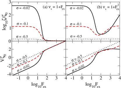
Figure 1: Force-dependent friction coefficient (upper panels) for different models of the damping $\nu_{s}(F_{ex})$ together with the steady-state velocities (lower panels). $\sigma$ specifies the distance from the glass-transition point in the schematic model.

The force-dependent friction of the probe exhibits three characteristic regimes. For small pulling forces in both models, the friction coefficient is constant, or equivalently, the average velocity of the probe is proportional to the external pulling force. This region extends to external forces of order unity and describes a linear response. When approaching the glass transition, the friction increases drastically as the correlation functions in Eq. (6) extend to increasingly longer time scales. Starting around $F_{ex}\approx 1$, the linear-response regime ends and gives rise to shear thinning: The friction decreases and it is proportionally easier to pull the particle. Equivalently, the average velocity of the intruder increases faster than linear with external force. For the model in the left panel of Fig. 1, the friction $\zeta$ approaches the limiting value given by the bare friction $\zeta_{0}$ and remains there for yet higher forces. This model hence describes behavior similar to the colloidal results for Newtonian microscopic dynamics. For the model in the right panel of Fig. 1, the friction approaches a minimum around $F_{ex}\approx 100$ and starts increasing for higher pulling forces.

In comparison, the models in Fig. 1(a) and Fig. 1(b) are almost equivalent in the linear-response and shear-thinning regimes, where the friction in Eq. (6) is dominated by the memory effects leading to a slowing down of the relaxation. The difference in the microscopic damping $\nu_{s}$ does not play a significant role. In contrast, for large pulling forces, the correlation function $\phi_{s}(t)$ relaxes to zero rapidly and the integral (6) is dominated by the short-time part of the correlation functions.

II.2 Comparison with simulation data

We adopt with $\nu_{s}=1+F_{ex}^{2}$ the second schematic model to compare with the simulation data in detail. The simulation setup is the same as described in Fiege et al. (2012): in a bidisperse mixture of hard spheres with size ratio $R_{s}/R_{b}=4/5$ of small to big particles and a respective mass ratio $m_{s}/m_{b}=16/25$, an intruder of radius $R_{0}=2R_{s}$ and mass $m_{0}=4m_{s}$ is suspended. Lengths and masses are measured such that $R_{s}=1$ and $m_{s}=1$ and a time scale is set by requiring T=1 in the system with $F_{e}x=0$, i.e. the random driving balances the dissipation by bare friction and collisions. Figure 2 shows the fit of the measured correlation functions by the model. The numerical solution of the density autocorrelator of the intruder fits quite well the corresponding simulation data for the moderately high force $F_{ex}=250$. For the smaller force $F_{ex}=1$, it shows some deviations. The fitting parameters are $v_{A}=200$ , $\sigma=-0.05$ for $\varepsilon=0.9$ as well as (not shown in Fig. 2) $v_{A}=300$, $\sigma=-0.09$ for $\varepsilon=0.7$ and $v_{A}=600$, $\sigma=-0.13$ for $\varepsilon=0.1$. The other parameters are the same as the ones mentioned above.

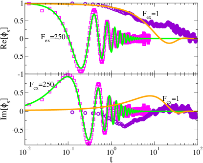
Figure 2: Comparison between the schematic model and the simulation data for the density autocorrelator of the probe particle at fixed packing fraction $\varphi=0.8$ and energy dissipation $\varepsilon=0.9$. The pulling forces are $F_{ex}=1$ and 250. The dashed lines represent the simulation data, the solid lines are the descriptions by the schematic model.

The corresponding fit of the friction coefficients is given in Fig. 3. In the regime of small forces, the schematic model shows a linear-response plateau. The simulation data also show a plateau for small forces (see Fig. 3 in Fiege et al. (2012)). As the glass transition is approached, this regime moves to smaller forces, so that it is visible in Fig. 3 only for the smallest $\varepsilon=0.1$ which is further away from the glass transition than $\varepsilon=0.9$ and $0.7$. However for $\varepsilon=0.1$ and $\varphi=0.8$ the simulations become increasingly difficult for small forces due to the occurrence of long lasting contacts. Hence the error bars become comparable to the result itself. For large pulling forces, the model shows qualitatively how the increasing friction coefficient can be rationalized within a schematic model. While the schematic model exhibits different limits for varying distances from the glass transition, the simulation data follow the same curve for $F_{ex}\gtrsim 500$. Between the extreme regimes of large and small pulling forces the friction coefficient exhibits a minimum that is similar for all distances from the glass transition for both the schematic model and the simulation.

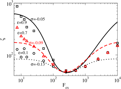
Figure 3: Effective friction of the intruder for different energy dissipation $\varepsilon=0.9$, 0.7 , and 0.1 at fixed packing fraction $\varphi=0.8$ of the host fluid. Individual data points show the simulation results, curves represent the results from the schematic models.

While the schematic model may only qualitatively fit the simulation data for the friction coefficient in Fig. 3, in addition to the good agreement of the correlation functions in Fig. 2 the results are also consistent with the predictions from MCT for hard spheres Kranz et al. (2010); Sperl et al. (2012); Kranz et al. (2013). For smaller dissipation, i.e. larger coefficient of restitution $\varepsilon$ in Fig. 3, the data can be described only by choosing points closer to the glass-transition line in the schematic model. Smaller distances to the glass transition given by smaller values of $\sigma$ indicate that for the same density of $\varphi=0.8$ the data for $\varepsilon=0.9$ are much closer to the glass transition than for $\varepsilon=0.1$ with $\varepsilon=0.7$ located in between. This finding is in agreement with the predicted increase of the glass-transition density with decreasing $\varepsilon$ within MCT Kranz et al. (2010); Sperl et al. (2012); Kranz et al. (2013).

III Kinetic Theory in low density limit

To clarify the origin of the scaling law $\zeta\propto\sqrt{F_{ex}}$ in the large-force asymptote, we propose a simple kinetic theory in the following. The simulation result from Fiege et al. (2012) has shown that the scaling law is independent of packing fraction. Therefore, a potential explanation of the increased friction by jamming or shear thickening seems unlikely. Also, the correlation functions for large pulling forces decay relatively quickly, cf. Fig. 2, also contradicting a buildup of long-time glass-like contributions to the integrals like in Eq. (6). In the following we shall therefore focus on the low density limit, where exact solutions can be obtained.

The formal solution of $\bm{v}(t)$ in Eq. (1) can be readily obtained and the corresponding ensemble average of the velocity of the intruder is given by

$$\big{\langle}\bm{v}(t)\big{\rangle}=\frac{\bm{F}_{ex}}{\zeta_{0}}\big{(}1-e^{-\frac{\zeta_{0}}{m}t}\big{)}+\frac{e^{-\frac{\zeta_{0}}{m}t}}{m}\int_{0}^{t}e^{\frac{\zeta_{0}}{m}t^{\prime}}\big{\langle}\bm{f}_{int}(t^{\prime})\big{\rangle}dt^{\prime}$$ (7)

where we have averaged out the initial velocity and the random force: $\big{\langle}\bm{v}_{0}\big{\rangle}=0$ and $\big{\langle}\bm{\eta}(t)\big{\rangle}=0$.

The direct calculation of $\big{\langle}\bm{f}_{int}(t)\big{\rangle}$ in Eq. (7) is difficult. The key point of our kinetic theory is to introduce the mean free path of the intruder, $l_{0}=\rho^{-1}\sigma_{cr}$, where $\rho=N/V$ is the particle number density and $\sigma_{cr}$ is the intruder’s cross section, which for hard sphere reduces to $\sigma_{cr}=4\pi R^{2}$. Let us denote the collision time as $t_{c}$. Between two successive collisions $nt_{c}<t<(n+1)t_{c}$, there is no interaction force in the hard sphere limit, $\big{\langle}\bm{f}_{int}(t)\big{\rangle}=0$. On average, after $t_{c}$ a collision event causes a momentum transfer from the intruder to its collision partner of the order of the intruder’s complete momentum. The velocity of the intruder increases again from almost zero due to the constant pulling force. Statistically, the intruder’s velocity exhibits periodic motion. Consider the motion of the probe in the first period: The average velocity reads

$$\big{\langle}\bm{v}(t)\big{\rangle}=\frac{\bm{F}_{ex}}{\zeta_{0}}\big{(}1-e^{-\frac{\zeta_{0}}{m}t}\big{)},\quad 0\leq t\leq t_{c}\,,$$ (8)

and the displacement of the motion satisfies

$$l_{0}=\Big{|}\int_{0}^{t_{c}}\big{\langle}\bm{v}(t)\big{\rangle}dt\Big{|}=\frac{F_{ex}}{\zeta_{0}}\big{[}t_{c}-\frac{m}{\zeta_{0}}(1-e^{-\frac{\zeta_{0}}{m}t_{c}})\big{]}\,.$$ (9)

The average velocity of the probe is given by

$$\big{\langle}v_{s}\big{\rangle}=\frac{1}{t_{c}}\Big{|}\int_{0}^{t_{c}}\!\big{\langle}\bm{v}(t)\big{\rangle}dt\Big{|}=\frac{l_{0}}{t_{c}}\,.$$ (10)

In general the friction of the probe $\big{\langle}v_{s}\big{\rangle}$ can be calculated by Eqs. (9,10) exactly. We first consider the two limiting cases $t_{c}\gg\frac{m}{\zeta_{0}}$ (overdamped limit) and $t_{c}\ll\frac{m}{\zeta_{0}}$ (ballistic regime).

In the overdamped limit, velocity relaxation dominates over collisions and the collision times are large,

$$t_{c}=\frac{l_{0}\zeta_{0}}{F_{ex}}\gg\frac{m}{\zeta_{0}}$$ (11)

or equivalently,

$$\frac{F_{ex}}{\zeta_{0}^{2}}\ll\frac{l_{0}}{m}.$$ (12)

The average velocity and the friction of the intruder can be obtained by Eq. (10) and definition of the friction itself, yielding

$$\big{\langle}v_{s}\big{\rangle}=F_{ex}/\zeta_{0},\quad\zeta=\zeta_{0}\,.$$ (13)

The friction experienced by the intruder is dominated by the effective friction originating from the medium.

In the ballistic limit, collisions dominate over velocity relaxation. Expanding $e^{-\frac{\zeta_{0}}{m}t}$ in Eq. (9) to second order, we get

$$t_{c}=\sqrt{\frac{2ml_{0}}{F_{ex}}}\ll\frac{m}{\zeta_{0}}\,.$$ (14)

The ballistic limit is given by the presence of pulling forces very large compared to the bare friction,

$$\frac{F_{ex}}{\zeta_{0}^{2}}\gg\frac{2l_{0}}{m}.$$ (15)

The average velocity and the friction of the probe are

$$\begin{split}\big{\langle}v_{s}\big{\rangle}&=\sqrt{\frac{l_{0}F_{ex}}{2m}}\propto\sqrt{F_{ex}}\\ \zeta&=\sqrt{\frac{2mF_{ex}}{l_{0}}}\propto\sqrt{F_{ex}}\,.\end{split}$$ (16)

Both the velocity as well as the friction are proportional to the square-root of the external pulling force and independent of the bare friction.

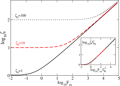
Figure 4: Force-friction relation at large forces for different damping in the low-density limit.

The general solution of Eqs. (9,10) can be calculated in parametric form and is given in Fig. 4, where the crossover is shown for the friction coefficient from a constant (linear large-force behavior of the velocity) to the square-root increase (square-root increase of the velocity for large forces). The reason why for a driven granular system the friction of the probe increases as $\zeta\propto\sqrt{F_{ex}}$ in the large-force regime but for colloidal hard-sphere systems, the friction only decreases to a constant value can be explained as follows. For different bare frictions $\zeta_{0}$, the $F_{ex}$-$\zeta$ plots can be rescaled as $F_{ex}/\zeta_{0}^{2}$ versus $\zeta/\zeta_{0}$, cf. the inset in Fig. 4. The behavior of the probe in the large-pulling-force regime is determined by the ratio of the collision time scale over the Brownian velocity relaxation time scale, $t_{c}/\frac{m}{\zeta_{0}}$, or equivalently the value of the rescaled force $F_{ex}m/(\zeta_{0}^{2}l_{0})$. In a driven granular system, the bare friction is quite small compared with the one in a Brownian suspension, $\zeta_{0}=1$ in the granular simulation Fiege et al. (2012) and $\zeta_{0}=50$ in the colloidal one Gnann et al. (2011). Indeed, one would also obtain the same asymptotic behavior $\zeta\propto\sqrt{F_{ex}}$ for Brownian systems for extremely large pulling forces.

IV Conclusion

We have investigated the microrheology of the driven granular hard sphere system by a schematic model and a simple kinetic theory. For small and moderate external pulling forces, the schematic model agrees reasonably well with the simulation data, cf. Fig. 3, and implies that the glass-transition density increases with smaller coefficient of restitution $\varepsilon$, confirming predictions from mode-coupling theory Kranz et al. (2010); Sperl et al. (2012); Kranz et al. (2013). For large forces, glassy dynamics becomes irrelevant and a simple kinetic theory clarifies the origin of the scaling of the friction with increasing pulling force. When damping by a surrounding fluid dominates the motion of the intruder at high forces, a second linear emerges where the friction becomes constant. When collisions dominate, the friction increases in a square-root law, $\zeta\propto\sqrt{F_{ex}}$.