Top Down Approach to Detect Multiple Planes in Images

Abstract

Detecting multiple planes in images is a challenging problem, but one with many applications. Recent work such as J-Linkage and Ordered Residual Kernels have focussed on developing a domain independent approach to detect multiple structures. These multiple structure detection methods are then used for estimating multiple homographies given feature matches between two images. Features participating in the multiple homographies detected, provide us the multiple scene planes. We show that these methods provide locally optimal results and fail to merge detected planar patches to the true scene planes. These methods use only residues obtained on applying homography of one plane to another as cue for merging. In this paper, we develop additional cues such as local consistency of planes, local normals, texture etc. to perform better classification and merging. We formulate the classification as an MRF problem and use TRWS message passing algorithm to solve non metric energy terms and complex sparse graph structure. We show results on challenging dataset common in robotics navigation scenarios where our method shows accuracy of more than 85 percent on average while being close or same as the actual number of scene planes.

I Introduction

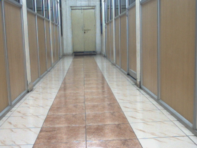
Detecting multiple planes in images is a challenging problem. If done accurately, it can provide strong cues to efficiently perform many vision tasks. Previously, Kähler and Denzler [6, 7], Zhou et al. [11] demonstrated the use of multiple planes for 3D reconstruction. Zhou et al. also exploit multiple planes for video stabilization [12]. Pham et al. develop an augmented reality application using multiple planar regions of images [9]. Kumar and Jawahar use multiple planes to guide camera positioning for robot manipulators [8]. To find planes, these methods use: $(i)$ manual annotation [7] or, $(ii)$ iterative RANSAC methods [7, 11] or, $(iii)$ fit planes in the 3D reconstructed output (easier than detecting the planes in images) [12]. We leverage recently developed multiple structure detection methods and build a sophisticated approach to identify multiple planes given two images. Our approach gives good results on challenging datasets (few are shown in Figure 1), on which the methods discussed above either fail or work, but use extra information in the form of 3D reconstruction.

In most of the applications discussed above viz. 3d reconstruction, augmented reality, video stabilization etc. more than one image of the planar scene is available. In this paper, we focus on the problem of detecting multiple planes given two images (i.e. an image pair). Given this setting we can compute stable features such as SIFT, SURF and also find feature matches between the two images. These matches can then be used to compute a homography, which encodes the transformation between planar region seen in the image pair. There are robust RANSAC based methods, for estimating a single homography, a survey of these methods can be found in [1]. Estimating a single homography typically gives us only the single most dominant planar region in the image. To find multiple planar regions, we need to estimate multiple homographies from the feature matches.

Figure 1: Multiple Plane detection from images. Top Left Initial Image to be segmented. Top Right Initial planar patches detected from ORK. Bottom Left Refined patches after distance based segmentation of planes Bottom Right Multiple planes detected corresponding to scene planes after optimal MRF labelling.

Initially, multiple homography estimation was performed using iterative methods. These methods eliminated the inliers of homography estimated for current iteration and again performed homography estimation on remaining matches. They typically need a priori knowledge of number of homographies/planes, otherwise we do not know when to terminate the iterative procedure. Also, the errors get compounded if a few wrong inliers are removed in the initial iterations and we end up achieving spurious results. More recently, sophisticated multi-structure detection methods have been developed by Toldo and Fusiello [10], Chin et al. [2], Pham et al. [9] and Jain and Govindu [5]. These methods bootstrap by randomly generating many hypotheses that fit a subset of data. The individual data points (in our case feature matches) are then associated with all the hypothesis (in our case homographies) that they fit well. The data points are then clustered into multiple structures based on the similarity of the set of hypothesis that they match to. The underlying idea is data points belonging to the same structure will show a preference to the same hypotheses from our initial sampled set. These multiple structure detection methods are domain independent and they show remarkable results when applied to problems such as multiple 2d-line fitting, multiple 2d-circle fitting, multiple 3d-plane fitting etc. When we use these methods for our problem of multiple homography estimation, we see that these methods at best provide us with multiple small planar patches (after some post processing), far exceeding the number of planes in our image pair. We use realistic scenes for all our experiments. This difference in performance is a result of sampling homographies that fit nearby points and also, there being more ambiguity in the problem of homography estimation as compared to curve fitting.

After detecting multiple structures, typically some hueristic merging methods are used. These methods merge two homographies provided the residual error after merging is small. These methods do not work well in practice, this is demonstrated by the experiments done in Section III D. In our work, we develop a novel alternative to merge the planar patches output by multiple structure detection methods. We use homography decomposition to associate estimated homographies of planar patches to their normals in 3d world. At this stage, some planar patches have incorrect normals and cannot be trivially merged. We propose an MRF model using TRWS to achieve the merging. Each feature match is assigned a random variable, which can take labels corresponding to initial patches. We arrive at an optimal labelling of the feature matches by minimizing an energy function defined over these random variables. Using texture and locally computed normals in our energy minimization function, we show that we are able to assign correct labels to feature matches that span large scene planes. This is primarily because we incorporate local normals in our MRF formulation, majority of which are correctly oriented despite the normal of the entire patch being incorrect. Also, our smoothness term in the MRF formulation ensures that labels assigned to a feature match are consistent with its neighboring matches. As discussed in section IV, we show good results on challenging datasets and compare our performance to other state-of-the-art multiple plane detection methods.

II Related Work

Figure 2: Scene planes detected for corridor, corner dataset respectively (from left). Connected meshes with the same color indicate matches that are grouped together as belonging to one plane by [2].

RANSAC based homography estimation methods have been extended to the problem of detecting multiple planes by removing inliers and re-estimating new homographies iteratively. Further, Zuliani et al. [13] developed a multi-RANSAC algorithm that is capable of estimating all homographies simultaneously. These methods do not work well in practice and also, need additional knowledge of number of planes.

II-A Methods using J-Linkage

Recently, sophisticated algorithms which do not require prior knowledge of number of planes have also been developed. Toldo and Fusiello [10] develop one such algorithm called J-Linkage. For homography estimation, J-Linkage starts by generating $M$ homographies from randomly sampled nearby feature matches. For each feature match, a preference set of the homographies (out of the $M$) that fit to the match within a threshold $\epsilon$ is created. A clustering step that starts with all matches in separate clusters is performed. The clustering step iteratively merges the feature matches that have similar preference set using the Jaccard Distance measure ($d_{J}(X,Y)=\frac{|X\cup Y|-|X\cap Y|}{|X\cup Y}$). This clustering step proceeds till the minimum $d_{J}$ is $1$, i.e. the preference set of all clusters have no more overlap. The outlier feature matches are also present as small clusters and these are eliminated by setting a threshold on cluster size.

Fouhey et al. [3] observe that J-linkage uses only nearby feature matches to generate initial homographies. This is done to ensure that the computed homographies correspond to real scene planes. Though, the downside of such an approach is that the homographies output by J-linkage are also locally optimal and do not fit a large scene plane. The scene plane is output as multiple small planar patches by J-linkage. Fouhey et al. [3] solve this by continuing to cluster the matches (after J-linkage) using the distance measure:

$d_{F}(X,Y)=\frac{1}{|X\cup Y|}\sum\limits_{c\epsilon X,Y}err_{H^{\prime}}(c)$

II-B Methods using Ordered Residual Kernel

Another category of multiple structure detection algorithms based on ordered residues have been formulated by Chin et al. [2]. For the problem of multiple homography estimation, again these methods start by randomly sampling $M$ homographies. Residues ($x^{\prime}-Hx$) are then computed for each feature match and homographies are ordered on the basis of increasing residue for each feature match. Thus, given a data point $\theta_{i}$ we obtain ordered homographies $\lambda^{i}_{1}$ (minimum residue) to $\lambda^{i}_{M}$ (maximum residue):

$\tilde{\theta_{i}}=\{\lambda^{i}_{1},\lambda^{i}_{2},\lambda^{i}_{3},...,\lambda^{i}_{M-1},\lambda^{i}_{M}\}$

An Ordered Residual Kernel (ORK), $k_{r}$, is defined between two data points:

$k_{r}(\theta_{i1},\theta_{i2})=\frac{1}{Z}\sum\limits_{t=1}^{M/h}z_{t}k^{t}_{\cap}(\tilde{\theta_{i1}},\tilde{\theta_{i2}})$

$k^{t}_{\cap}$ is the Difference of Intersection Kernel (DOIK) defined on the homographies ordered by residues ($\tilde{\theta_{i1}}$ and $\tilde{\theta_{i2}}$) of the two data points.

$k^{t}_{\cap}=\frac{1}{h}(|\tilde{\theta_{i1}}^{1:\alpha_{t}}\cap\tilde{\theta_{i2}}^{1:\alpha_{t}}|-|\tilde{\theta_{i1}}^{1:\alpha_{t-1}}\cap\tilde{\theta_{i2}}^{1:\alpha_{t-1}}|)$

Figure 3: Planar patches obtained after the distance based refinement step for corridor and corner dataset. In comparison to Fig 2, the images show that our distance based refinement step is able to cut the detected scene planes (that spanned two or more real world planes) into smaller planar patches (that span only a single scene plane).

The ORK is a weighted sum of the difference in number of intersecting homographies taken over some step size $h$. This kernel is a valid mercer kernel and induces a mapping of the data points to a Reproducing Kernel Hilbert Space (RKHS). Chin et al. show that data points belonging to the same structure form clusters in this RKHS. They use kernel PCA and spectral clustering to detect these structures. To minimize the number of structures detected after this step, they also give a structure merging scheme. This merging scheme sequentially merges structures if the overall residue after merging is below a threshold. The merging continues till all the data can be explained satisfactorily by identified structures (i.e. sum of all residues is bounded).

Like Fouhey et al. [3], we propose an alternative scheme for merging structures output by the multiple structure detection methods.We compare the performance of our approach to Fouhey et al. [3] and the domain independent merging scheme given by Chin et al. [2].

III Our Approach

The following sections describe the different steps of our approach.

III-A Initial Planar Patch Estimates

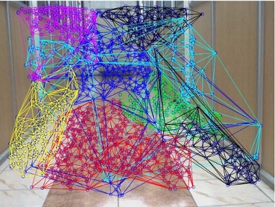
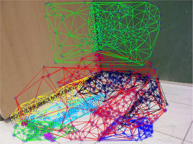
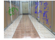
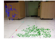
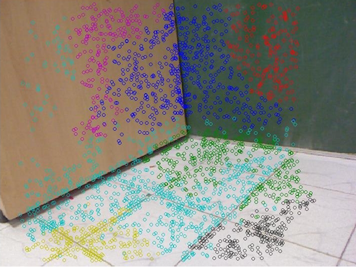
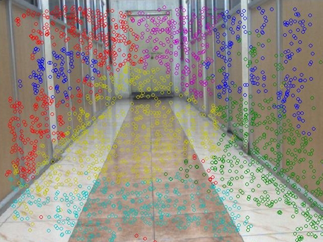
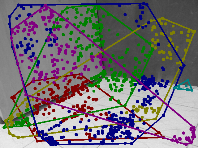
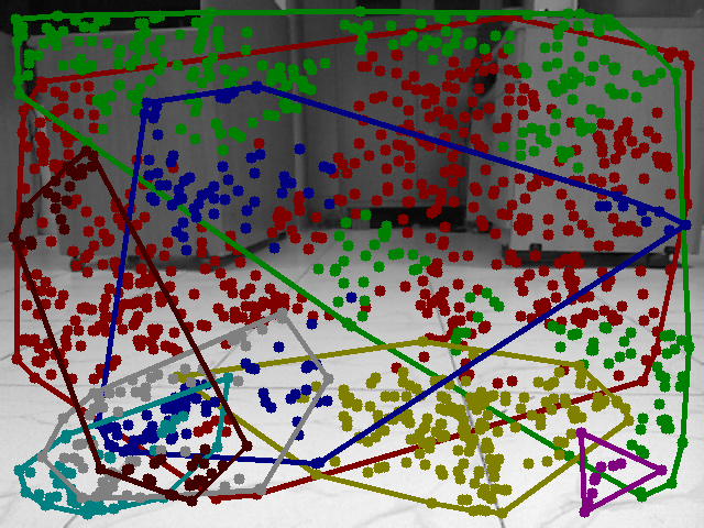
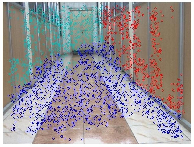
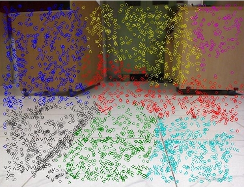
Given two images we compute SURF features and obtain feature matches. On obtaining these matches, we use the multiple structure detection method described in section II-B for estimating multiple homographies and hence, multiple scene planes. We perform the steps of: $(i)$ computing ordered residues of feature matches, $(ii)$ using the ordered residual kernel, $(iii)$ performing kernel PCA and spectral clustering. We avoid using the cost of residues based structure merging scheme given by Chin et al. [2]. We justify in Section III-D that such schemes do not work well in practice. Refer [2] for more details of this method. Figure 2 shows the scene planes that are found by using this method on two datasets: $(i)$ corridor, consisting of $4$ planes and $(ii)$ corner, consisting $3$ planes representative of a corner of a cuboid. As seen in Figure 2, the detected planes have two major problems:

Firstly not all detected planes correspond to a planar patch. For example, the blue mesh in corridor dataset shows that the detected plane spans left as well as right plane, the $2$ red meshes in corner dataset show that $2$ detected planes span ground and left, right and left planes respectively.Also,the number of planes detected by the multiple structure detection method exceeds the number of true scene planes.

Figure 4: The minimum and second minimum after applying the homography of one plane to feature matches of the other.

We solve these problems using the following pipeline:

• Distance based refinement of detected planes.

• Computation of plane normals.

• MRF based optimal labelling due to local and texture constraints.

III-B Distance Based Refinement of Detected Planes

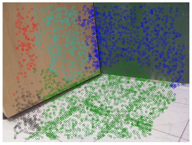
In this step, we first perform a delaunay triangulation on the feature matches. If the detected plane has feature matches from multiple scene planes, chances are these would be at a larger distance from each other. We set a threshold on distance and cut the delaunay mesh into smaller meshes (when any side exceeds the distance threshold). This step, to some extent, separates the planes output by multiple structure detection method into smaller planar patches. These smaller planar patches have stable properties as compared to detected planes which spanned multiple true scene planes. The results of performing this step on corridor, lab dataset are shown in Figure 3.

III-C Plane Normal Computation

Planar points between two images are related by homography. Homography is a relation between the plane and the relative pose between the images which can be decomposed [11] to find the plane normals.

$H=(R+\frac{TN^{t}}{D})$

where N is the plane normal and D is the perpendicular distance between the plane and camera. We have found that in cases of perspective motion between the camera and the plane, in presence of multiple planes, the decomposition is mostly erroneous due to the bilinear nature of the normal and translation term .We also discard planes formed by less than 10 points as they are mostly erroneous.

III-D Residue Based Merging of Detected Planes

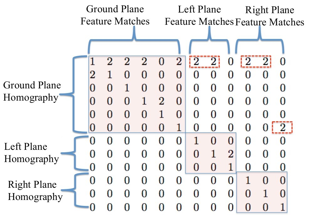
Typically methods of detecting multiple homographies, including Chin et al. resort to merging the detected planes by applying the homography of one to other. The merging is done, if the residue after applying the homography of another plane is below a threshold. We design an experiment, where we perform the above on: $(i)$ planar patches out put by Chin et al. before doing the merging and $(ii)$ on planar patches that are manually marked, these planes have desirable properties (viz. they span entire planar region). As shown in Figure 4, for $(i)$ we have $6$ ground, $3$ left and $3$ right planes. For $(ii)$, we have use $10$ ground, $10$ left and $10$ right planes. We create a matrix where the rows indicate the homography taken and columns indicate the plane to which it is applied. We mark out the first and second minimum residues by $1$ and $2$ in this matrix. The second minimum residue will dictate the merging in residues based merging approach. In ideal conditions, all the $1$’s and $2$’s should lie in the shaded regions of Figure 4. This is the case for controlled experiment $(ii)$, but not for $(i)$ (5 out of 12 planes marked in red have second minimum residues for incorrect homographies). Since our experiments show that using residues alone is not sufficient, especially for multiple structure detection methods like Chin et al., we develop other cues that can be exploited to achieve merging.

III-E Top Down Approach

Based on the discussion above, we propose exploiting the local consistency constraint (viz. same direction of normals, similar texture etc.), that should hold for a planar patch, to merge scene planes. We consider each feature match in its local neighbourhood ($k$ nearest neighbours in detected planar patch) to form a small local planar patch. This is in cognizance to local patches embodying a scene plane [3]. With our decompostion to local planar patches, we can now compute local surface normal for each such planar patch. The consistency in orientation of local normals spanning a single scene plane is an important cue, so is its texture. We use these cues to refine and recompute association of feature matches to the detected planes. Note that we do an MRF optimization on a sparse graph of only feature matches and not a dense graph of all pixels. Such dense graphs are common in image segmentation literature. We call our approach a top-down approach, because we resort to feature matches and local planar patches to merge detected planes, after having performed one step of planar patch detection (using multi-structure detection methods). For our approach it is necessary to perform an initial multiple structure detection step. Because we assume that the true structure is present in the output of multiple structure detection method and develop a method to merge the detected structures to these true structures.

III-F Graph Optimization

The feature matches are connected to form a graph using delaunay triangulation. This graph structure is formulated as Markov Random Field where the goal is to assign each feature match a maximal posterior probability (MAP) label. This label is one out of the detected planes by multiple structure detection step. As a common practice [16], instead of direct probability maximization, we minimize the energy as discrete labelling problem on the graph in the form of Eqn1.

$$\textbullet E_{MRF}=\sum_{X}E(p,{l\epsilon L})+\sum_{x}\sum_{q\epsilon N(X)}E(p,q)$$ (1)

In the above equation, L = $(p^{1}..p^{n})$ is the set of labels where $n$ is the number of initial planar patches obtained from initial planar patch estimate step. The set $N(X)$ is the neigbourhood of the node X. The $E(p,l)$ defines the unary energy potential. It determines the likelihood of the feature match corresponding to a scene plane labelled $l$ output by multiple structure detection step. $E(p,q)$ defines the pairwise energy potential which represents the graph similarity of the neighbourhood.

III-G Unary Energy Term

Unary energy is defined by us as a sum of energies relating to residues of local planar patch and normal similarity between feature and plane.

$$E_{unary}=E(X)_{normal}+E(X)_{residual}$$ (2)

Figure 5: This figure compares the results of different multiple plane detection methods on different datasets. Datasets - box, corner, corridor and tables (from left to right). From top to bottom, each row corresponds to the following methods - Chin et al. [2], Fouhey et al.[3] and our approach.In our approach to corridor we undersegment as the normal on the perspective plane doesnt turn out well also the tracks are not good

III-G1 Residue of local planar patch

Each feature match has a local planar patch defined around it using $k$ nearest neighbours. Our energy is the sum of residues of this local patch with respect to the parameters of the patch labelled $l$.

$$E(X,l)_{residual}=\sum_{X\epsilon P}||(X^{\prime}-H_{l}X)||_{L2}$$ (3)

Here $P$ represents the local planar patch. We use $k=10$ as smaller patches can be erroneous while decomposition.These nearest neighbours are members of the same planar patch found initially as this implies that they are part of a larger plane rather than some local surface fit to a scene.

III-G2 Normal Similarity measure

The local normal of each feature match should ideally be aligned with the normal of the scene plane. So the energy term for each feature decreases if it aligns with the plane labelled $l$.

$$E(X,l)_{normal}=(1-\frac{N_{X}.N_{l}}{|N_{X}||N_{l}|})^{2}$$ (4)

III-H Pairwise Energy Terms

Pairwise energy defined by us consists of three terms similarity measure, mutual plane consistency and texture similarity.

$$E_{binary}={\lambda_{1}}E(X,Y)_{sm}+{\lambda_{2}}E(X,Y)_{mp}+{\lambda_{3}}E(X,Y)_{ts}$$ (5)

where $\lambda_{1}$ … $\lambda_{n}$ are the weights of pairwise terms.

III-H1 Similarity Measure

We use the standard Potts Model where the neighbouring edges with different labels are penalized. Initially each feature is assigned the label of the initial planar patch to it belongs.

$$E(X,Y)_{sm}=\left\{\begin{array}[]{rl}1&\mbox{ if $p_{X}\neq p_{Y}$}\\ 0&\mbox{ otherwise}\par\end{array}\right.$$

(6)

III-H2 Mutual Plane Consistency

Neighbouring features should have similar surface normals, utilizing this constraint we find the measure.

$$E(X,Y)_{mp}=(1-\frac{N_{X_{p}}.N_{X_{q}}}{|N_{X_{p}}||N_{X_{q}}|})^{2}$$ (7)

III-H3 Texture Similarity

This measure takes into account the local texture between neighbours should be similar. Here we compare the mean of a image patch around each feature match with its neighbour. We use a $5\times 5$ patch centered at the feature. This term brings in the smoothness of texture across a plane, typically common in images.

$$\hskip 56.9055pt\mu=\frac{\Sigma_{WS}(R,G,B)}{WS}\hskip 14.22636pt:WS=WindowSize$$ (8)

$$E(X,Y)_{cs}=||(\mu_{p(x)}-\mu_{p(y)})||_{L2}$$ (9)

This combination of energy terms segments out the planes robustly. We choose Tree Weighted Sequential(TRWS)[15] message passing algorithm to solve the optimization problem.

This method is similar to Loopy Belief Propagation and solves on the priniciples of linear programming and its duality for NP hard MRFs. The method has experimentally shown better results than LBP while working well in cases of non metric pairwise terms. It also finds the lower bound of the energy which acts as a guidance for convergence.Thus this method provides flexibility to include varied and sophisticated energy terms with complex graph structures. [14]

IV Experimental Results

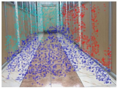
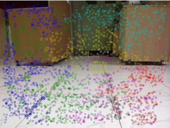
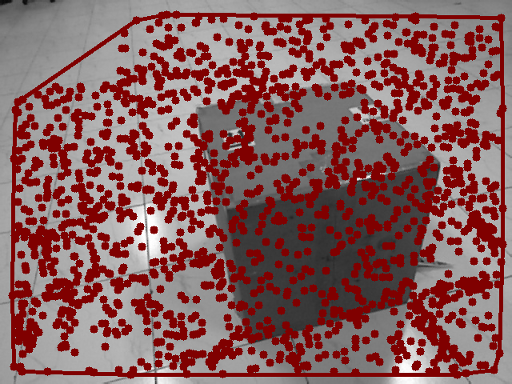
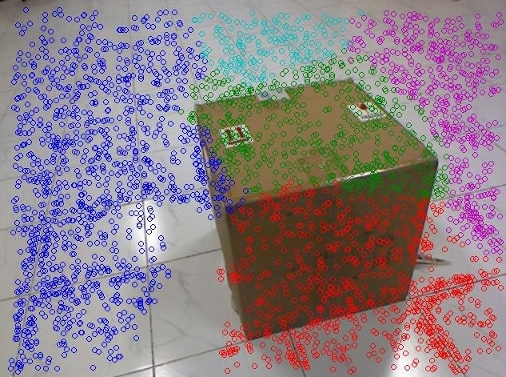
We evaluate our approach on various images taken in an indoor environment. The images of our datasets and the results of different methods for multiple plane detection on them have been shown in Figure 5. Our images are representative of scenes that will be encountered by a robot in SLAM setting and also in other 3d reconstruction methods. These datasets are challenging because some of our planes have multiple textures (ground plane of corridor) and a specular reflection (glass in the left and right planes of corridor, ground plane of box). The images have been taken from a dataset captured for VSLAM by a Flea2 camera mounted on P3Dx robot. There is considerable movement between the images ($\approx$ around $20cm$ for corridor dataset and for others it is in the range of $5$ to $10$cm, with 2 to 5 degrees rotation). We compute SURF features and use the KLT tracker to find feature matches. The average number of feature matches found is around 3000. These features generally encompasses the image and the corresponding planes well.

We compare our approach to the two approaches – Fouhey et al. [3] and Chin et al. [2] – discussed in section II. For Fouhey et al. and Chin et al.  we use their publicly available code.For fairness we run the codes several times and the best results were taken .

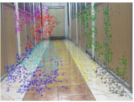
Using$1500$ SURF features tracked by KLT, code by Fouhey et al. took in the range of $5$ to $10$ mins per experiment. As can be seen from Figure 5, for corridor it finds erroneous planes. For box dataset, where there are parallel planes (with different textures) it labels both of them as same. Also, it fails to detect the front facing plane.It performs badly in such image as the data has high amount of outliers and purely residue based merging does not help. For the corridor and lab dataset it finds multiple planes spanning other planes as well as the number of planes is grossly oversegmented .

Taking this performance into consideration we do a quantitative and qualitative analysis of results only between ORK and our approach. We run both approaches with Multi Guided Sampling Pham et al . [9]. Table I shows Classification error of the data and number of planes detected in the image. Our approach shows competitive results for classification error while having a lower error for most of the data. The number of planes detected by ORK is more erroneous than ours as it over segments the same plane.

IV-A Quantitave Analysis

We show statistics for the PS (Amount of plane detected(PD) present in scene plane(SP)) and AD (The amount of planes detected(PD) spanning the scene plane(SP)). In an ideal situation both should correspond to 1. We show our results only for corridor and corner dataset(space constraints).Table II shows PS and AD for corridor dataset using our approach. For example first detected plane(PD I) from PS is detected primarily in second scene plane(SP II)(0.89) and from AD we can find that PD I covers entirely SP II (0.95) thus making both the ratios close to 1. In comparison ORK (Table III )has its PD I primarily (0.986) in SP I but the PD I covers only (0.16) of SP I showing the high error ratio while classification accuracy being high. Similar analysis of the whole data shows that our method performs far better than ORK in finding true scene planes.

IV-B Qualitative Analysis

Chin et al. perform better than Fouhey et al. for our datasets, but there is still scope for improvement. For the box dataset, the topmost plane (detected in blue) has a few other planes detected in between. Similar is the case with ground plane in the corner dataset, it is split into multiple planar patches. There are also erroneous planes viz. the plane marked by green feature matches in the corridor dataset. This plane has matches from the left as well as ground plane. Similarly, plane marked by blue in corner dataset spans the left and ground plane. We are able to solve these problems in our approach, since we impose strong locality constraints and also look at the local normals, texture to perform merging.

V Conclusion

In this work, we develop an MRF based top down approach to merge multiple small planar patches detected by multiple structure detection methods. We show significant improvement over previous methods. This improvement results from the fact that we bring in domain knowledge to the problem of multiple plane detection. Our domain knowledge is in the form of cues such as local normals, texture and local consistency of planes. We formulate an energy function using this domain knowledge and minimize it through an MRF optimization.

TABLE I: error matrix

METHOD		OUR		ORK
Dataset	No of Ground truth SPs	error(in ’%’)	No of SPs detected	error(in ’%’)	No of SPs detected
Lab	4	12.32	7	18.75	7
Corner	3	18.9	6	12.33	8
Box	3	13.24	5	13.53	6
Corridor	4	18.78	3	23.65	6

TABLE II: Corridor - Our Approach

PS	PD I	PD II	PD III
SP I	4.20	0	57.52
SP II	89.92	3.73	3.27
SP III	2.83	96.26	4.32
SP IV	3.03	0	34.87

AD	PD I	PD II	PD III
SP I	10.02	0	89.97
SP II	95.82	1.87	2.29
SP III	5.55	88.88	5.55
SP IV	11.69	0	88.30

TABLE III: Corridor ORK

PS	PD I	PD II	PD III	PD IV	PD V	PD VI	PD VII
SP I	98.86	0.38	10.63	56.10	3.48	11.31	7.19
SP II	0	0	88.75	28.77	1.93	33.94	85.61
SP III	1.13	99.61	0.60	8.01	89.92	20.43	7.19
SP IV	0	0	0	7.10	4.65	34.30	0

AD	PD I	PD II	PD III	PD IV	PD V	PD VI	PD VII
SP I	16.63	0.19	6.69	58.89	1.72	11.85	4.01
SP II	0	0	32.77	17.73	0.56	20.87	28.05
SP III	0.14	38.78	0.29	6.53	34.47	16.64	3.12
SP IV	0	0	0	16.31	5.02	78.66	0

TABLE IV: Corner

PS	PD I	PD II	PD III	PD IV	PD V
SP I	50.58	100.00	10.13	21.38	96.15
SP II	0	0	7.61	76.66	3.84
SP III	49.41	0	82.24	1.95	0

AD	PD I	PD II	PD III	PD IV	PD V
SP I	9.94	41.02	18.85	18.74	11.42
SP II	0	0	17.31	82.12	0.5587
SP III	5.90	0	93.05	1.04	0

TABLE V: Corner-ORK

PS	PD I	PD II	PD III	PD IV	PD V	PD VI	PD VII	PD VIII
SP I	33.74	98.92	0.86	0	0.61	5.05	91.87	66.81
SP II	0	0	87.82	100.00	96.71	77.04	2.50	19.91
SP III	66.25	1.07	11.30	0	2.66	17.89	5.62	13.27

AD	PD I	PD II	PD III	PD IV	PD V	PD VI	PD VII	PD VIII
SP I	25.46	12.26	0.26	0	0.4	1.73	19.60	40.26
SP II	0	0	15.94	23.83	37.17	15.62	0.31	7.10
SP III	70.75	0.18	4.90	0	2.45	8.67	1.69	11.32

References

- [1] A. Agarwal, C. V. Jawahar, and P. J. Narayanan. A survey of planar homography estimation techniques. Technical report, 2005.
- [2] T.-J. Chin, H. Wang, and D. Suter. Robust fitting of multiple structures: The statistical learning approach. In ICCV, pages 413–420, 2009.
- [3] D. F. Fouhey, D. Scharstein, and A. J. Briggs. Multiple plane detection in image pairs using j-linkage. In Int. Conf. on Pattern Recognition, 2010.
- [4] O. Haines and A. Calway. Detecting planes and estimating their orientation from a single image. In Proceedings of the British Machine Vision Conference, pages 31.1–31.11. BMVA Press, 2012.
- [5] S. Jain and V. M. Govindu. Efficient higher order clustering on the grassmann manifold. In ICCV, 2013.
- [6] O. Kähler and J. Denzler. Detecting coplanar feature points in handheld image sequences. In In Proceedings Conference on Computer Vision Theory and Applications, VISAPP 2007, pages 447–452. INSTICC Press, 2007.
- [7] O. Kähler and J. Denzler. Tracking and reconstruction in a combined optimization approach. IEEE Transactions on Pattern Analysis and Machine Intelligence, 34(2):387–401, 2012.
- [8] D. S. Kumar and C. Jawahar. Robust homography-based control for camera positioning in piecewise planar environments. In Computer Vision, Graphics and Image Processing, pages 906–918. Springer Berlin Heidelberg, 2006.
- [9] T.-T. Pham, T.-J. Chin, J. Yu, and D. Suter. The random cluster model for robust geometric fitting. In CVPR, pages 710–717. IEEE, 2012.
- [10] R. Toldo and A. Fusiello. Robust multiple structures estimation with j-linkage. In Proceedings of the 10th European Conference on Computer Vision: Part I, ECCV ’08, pages 537–547, Berlin, Heidelberg, 2008. Springer-Verlag.
- [11] Z. Zhou, H. Jin, and Y. Ma. Robust plane-based structure from motion. In CVPR, pages 1482–1489, 2012.
- [12] Z. Zhou, H. Jin, and Y. Ma. Plane-based content preserving warps for video stabilization. In CVPR, pages 2299–2306, 2013.
- [13] M. Zuliani, C. Kenney, and B. Manjunath. The multiransac algorithm and its application to detect planar homographies. In Image Processing, 2005. ICIP 2005. IEEE International Conference on, volume 3, pages III–153–6, 2005.
- [14] R. Szeliski,R. Zabih, D. Scharstein,O. Veksler,A. Agarwala,C. Rother. A comparative study of energy minimization methods for Markov random fields. In ECCV,pages 16–29, 2006.
- [15] V. Kolmogorov Convergent Tree-Reweighted Message Passing for Energy Minimization. In IEEE Trans. Pattern Anal. Mach. Intell.,pages 1568–1583, 2006.
- [16] Y. Boykov and V. Kolmogorov An Experimental Comparison of Min-Cut/Max-Flow Algorithms for Energy Minimization in Vision. In In IEEE Transactions on Pattern Analysis and Machine Intelligence (PAMI),, vol. 26, no. 9, pages 1124-1137, September 2004.