SI-HEP-2013-15 Applications of QCD Sum Rules
to Heavy Quark Physics

Abstract

In these lectures, I present several important applications of QCD sum rules to the decay processes involving heavy-flavour hadrons. The first lecture is introductory. As a study case, the sum rules for decay constants of the heavy-light mesons are considered. They are relevant for the leptonic decays of $B$-mesons. In the second lecture I describe the method of QCD light-cone sum rules used to calculate the heavy-to-light form factors at large hadronic recoil, such as the $B\to\pi\ell\nu_{\ell}$ form factors. In the third lecture, the nonlocal hadronic amplitudes in the flavour-changing neutral current decays $B\to K^{(*)}\ell\ell$ are discussed. Light-cone sum rules provide important nonfactorizable contributions to these amplitudes.

Introduction

The method of sum rules in quantum chromodynamics (QCD) developed in [1] relates hadronic parameters, such as decay constants or transition form factors, with the correlation functions of quark currents. Let me outline the three key elements of this method:

• Correlation function of local quark currents is defined. The simplest, two-point correlation function is formed by two quark-antiquark current operators sandwiched between the QCD vacuum states. This is a function of the 4-momentum transfer between the currents. In the region of large spacelike momentum transfers, the correlation function represents a short-distance fluctuation of quark-antiquark fields. The propagation of quarks and antiquarks at short distances is asymptotically free, the gluon exchanges being suppressed by a small QCD coupling. In addition, the interactions with “soft” (low momentum) quark-antiquark and gluon fields populating the QCD vacuum have to be taken into account.

• Operator-product expansion (OPE) of the correlation function is worked out. This expansion provides an analytical expression for the correlation function at spacelike momentum transfers, with a systematic separation of short- and long-distance effects. The former are described by Feynman diagrams with quark and gluon propagators and vertices, whereas the latter are encoded by universal parameters related to the nonperturbative QCD dynamics. In the case of two-point sum rules, these parameters are the averaged local densities of the QCD vacuum fields, the condensates. The contributions of vacuum effects in OPE are suppressed by inverse powers of the large momentum and/or heavy-quark mass scale, allowing one to truncate the expansion at some maximal power.

• Hadronic dispersion relation for the correlation function is employed. The basic unitarity condition allows one to express the imaginary part (spectral density) of the correlation function in terms of the sum and/or integral over all intermediate hadronic states with the quantum numbers of the quark currents. On the other hand, employing the analyticity of the correlation function in the momentum transfer variable, one relates the OPE result at spacelike momentum transfers to the integral over hadronic spectral density. In this way a link between QCD and hadrons is established, and the resulting relation between the OPE expression and hadronic sum is naturally called a “QCD sum rule”.

After this general description of the method, let me quote a shorter but more emotional definition of QCD sum rules: ”Snapshots of hadrons or the story of how the vacuum medium determines the properties of the classical mesons which are produced, live and die in the QCD vacuum”, given as a title to the review [2] written by one of the founders of this method.

Due to a vast amount of applications of QCD sum rules accumulated during many years, these lectures represent only a brief guide to the field, exemplifying applications to a few important processes involving heavy flavoured hadrons. More detailed reviews are listed in [2, 3, 4, 5, 6].

1 ​​​​​​. Lecture: Calculating the $B$-meson decay constant

In this introductory lecture, I consider, as a study case, the QCD sum rule derivation for an important hadronic parameter – the $B$-meson decay constant.

1.1 $B$-meson leptonic decays

         

(a)                                                      (b)

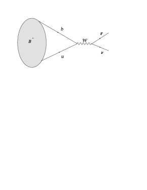
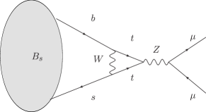
Figure 1: (a) Diagram of the weak leptonic decay $B^{-}\to\tau\bar{\nu}_{\tau}$; (b) one of the diagrams of the FCNC leptonic decay $B_{s}\to\mu^{+}\mu^{-}$. The initial $B$ meson is denoted by a blob.

The decay diagrams are shown in Fig. 1. The first leptonic decay is a weak transition $B^{-}\to\ell\bar{\nu_{\ell}}$ via virtual $W$ boson exchange. For $\ell=\tau$ its branching fraction was measured at $B$ factories [7]. The second decay, $\bar{B}_{s}\to\ell^{+}\ell^{-}$, is a rare flavour-changing neutral current (FCNC) transition generated by the loop diagrams with heavy particles ($t$,$Z$,$W$). Its recent observation at LHC [8] was a great experimental achievement. Although short-distance electroweak interactions are quite different, these decays have one common feature: the initial $B$-meson annihilates and the final state contains no hadrons i.e. it is a vacuum (lowest energy) state of QCD. The decay amplitude of the weak decay in Standard Model (SM):

$$A(B^{-}\to\tau^{-}\bar{\nu}_{\tau})=\frac{G_{F}}{\sqrt{2}}\,V_{ub}\,\bar{\tau}\gamma^{\mu}(1-\gamma_{5})\nu_{\tau}\langle 0|\bar{u}\gamma_{\mu}\gamma_{5}b|B^{-}\rangle\,,$$ (1)

contains the simplest possible hadronic matrix element

$$\langle 0|\bar{u}\gamma^{\mu}\gamma_{5}b|B(p_{B})\rangle=ip^{\mu}_{B}f_{B},$$ (2)

in which the local operator of $b\to u$ weak transition current is sandwiched between $B$ and the vacuum state. The above formula in terms of a constant parameter $f_{B}$ reflects the fact that $p_{B}^{\mu}$ is the only 4-momentum involved in this hadronic matrix element and $p_{B}^{2}=m_{B}^{2}$. The quantity $f_{B}$ is the $B$-meson decay constant we are interested in. In order to use the experimental measurement of the decay branching fraction:

$$BR(B^{-}\!\to\!\tau^{-}\bar{\nu}_{\tau})=\frac{G_{F}^{2}|V_{ub}|^{2}}{8\pi}m_{\tau}^{2}m_{B}\left(1-\frac{m_{\tau}^{2}}{m_{B}^{2}}\right)^{2}f_{B}^{2}\tau_{B^{-}}\,,$$ (3)

where $\tau_{B^{-}}$ is the lifetime of $B^{-}$, one needs to know $f_{B}$ from the theory. This will allow one to to extract the fundamental CKM parameter $|V_{ub}|$ or to check if there is an admixture of new physics, e.g., of a charged Higgs boson exchange, in this decay.

The rare leptonic decay, $B_{s}\to\mu^{+}\mu^{-}$ , is even more sensitive to new physics contributions, due to the presence of heavy particle loops. The corresponding hadronic matrix element

$$\langle 0|\bar{s}\gamma^{\mu}\gamma_{5}b|B_{s}(p_{B})\rangle=ip^{\mu}_{B}f_{B_{s}}$$ (4)

is very similar to Eq. (2), and the squared decay constant $f_{B_{s}}^{2}$ enters the decay width. The CKM suppressed $B_{d}\to\mu^{+}\mu^{-}$ decay contains the decay constant of $B_{d}$. Due to isospin symmetry between $u$ and $d$ quarks, $f_{B_{d}}\simeq f_{B_{u}}\equiv f_{B}$ with a good accuracy. On the other hand, $f_{B_{s}}$ and $f_{B}$ noticeably differ, because the $SU(3)_{flavor}$ symmetry is violated by the quark mass difference $m_{s}-m_{u,d}$. Hence, an accurate calculation of $f_{B_{s}}$ has to take into account the finite $s$-quark mass.

We conclude that a QCD calculation of $f_{B}$ is indispensable for disentangling the fundamental flavour-changing transitions from the measurements of leptonic $B$ decays.

1.2 $B$-meson decay constant in QCD

Figure 2: $B$ meson transition to vacuum.

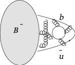
The task is to calculate the hadronic matrix element (2) which is shown in Fig. 2, separated from the electroweak part of the leptonic decay amplitude. The wavy lines and loops in this figure indicate gluons and quark-antiquark pairs interacting with the valence $b$ and $\bar{u}$ quarks inside $B^{-}$ meson. But these lines and loops are only illustrative: it is not possible to directly attribute QCD Feynman graphs to a hadronic amplitude.

The quantum field theory of quarks, gluons and their interactions is encoded in the QCD Lagrangian:

$$L_{QCD}(x)=-\frac{1}{4}G_{\mu\nu}^{{a}}G^{{a}\,\mu\nu}(x)+\sum_{q=u,d,s,c,b,t}\!\!\!\!\!\bar{q}^{\,i}(x)(iD_{\mu}\gamma^{\mu}-m_{q})q^{\,i}(x)$$ (5)

where $D_{\mu}=\partial_{\mu}-ig_{s}\frac{\lambda^{a}}{2}A^{a}_{\mu}$ is the covariant derivative, $G_{\mu\nu}^{{a}}=\partial_{\mu}A^{a}_{\nu}-\partial_{\mu}A^{a}_{\nu}+g_{s}f^{abc}A^{a}_{\mu}A^{a}_{\nu}$ is the gluon-field strength tensor and $g_{s}$ is the quark-gluon coupling, so that $\alpha_{s}=g_{s}^{2}/(4\pi)$, with summation over the colour indices $i=1,2,3$ and $a=1,...8$. From Eq. (5) one derives the basic elements of the QCD Feynman graphs: quark and gluon propagators and quark-gluon, 3-gluon and 4-gluon vertices. In QCD, a crucial role is played by quark-gluon loop diagrams generating the effective scale-dependent coupling $\alpha_{s}(\mu)$. As we know, it logarithmically decreases at large scales, $\mu\to\infty$, (asymptotic freedom) as illustrated in Fig. 3. The perturbation theory in terms of Feynman diagrams of quark-gluon interactions is well defined only at large energy/momentum transfers. Inversely, at small momenta (long distances), as shown in the same Fig. 3,

Figure 3: Dependence of the effective coupling in QCD on the energy/momentum scale $Q$.

the coupling grows. At momentum transfers smaller than a few hundred MeV the perturbation theory for quarks and gluons in QCD is senseless. An intrinsic scale $\Lambda_{QCD}\sim 200-300$ MeV emerges, the quarks, antiquarks and gluons interact strongly. Moreover, they are only observable in a form of coulourless bound states - the hadrons, one of them is the $B$ meson.

Another important feature of QCD concerns the vacuum state which is not an “empty space” in this theory. It contains fluctuating quark-antiquark and gluon fields with characteristic wave lengths of $O(1/\Lambda_{QCD})$. Averaged densities of these fields known as vacuum condensate densities play an important role in our story. In fact, the most important role will be played by the quark condensate with a density parametrized as the vacuum average of the Lorentz- and colour-invariant local operator $\langle 0|\overline{q}^{i}q^{i}|0\rangle\equiv\langle\bar{q}q\rangle\neq 0$, ($q=u,d,s$) with dimension $d=3$. Let me remind you that $\langle\bar{q}q\rangle\neq 0$ reflects the spontaneous breaking of chiral symmetry in QCD. One acquires a set of vacuum condensate densities with dimensions $d=3,4,5,..$ formed by all possible colourless Lorentz-invariant operators built from quark and gluon fields. E.g., the $d=4$ operator formed from two gluon-field strengths yields the gluon condensate density $\langle 0|(\alpha_{s}/\pi)G^{a}_{\mu\nu}G^{a\,\mu\nu}|0\rangle\equiv\langle GG\rangle\neq 0$. Importantly, there is no $d=2$ condensate in QCD. A review on vacuum condensates can be found in [9].

Returning to the process of $B$-meson annihilation, from the point of view of QCD it is important that the energy scale of quark-gluon interactions binding $b$ and $\bar{u}$ inside $B$ is characterized by the mass difference between the meson ($m_{B}\simeq 5.3$ GeV) and heavy $b$-quark:

$$\bar{\Lambda}\sim m_{B}-m_{b}\sim 500-700~{}\mbox{MeV}.$$ (6)

To quantify the above estimate we literally take $m_{b}=4.6-4.8$ GeV, the so called “pole” quark mass. Important is that quarks and gluons inside the $B$ meson have energies $\leq\bar{\Lambda}$ and hence interact strongly. At such scales no perturbative expansion in $\alpha_{s}(\bar{\Lambda})$ is possible and QCD Feynman graphs cannot be used. Moreover, in addition to ”valence” quarks, the partonic components with soft gluons and $\bar{q}q$ -pairs:

$$|B^{-}\rangle=|b\bar{u}\rangle\oplus|b\bar{u}G\rangle\oplus|b\bar{u}\bar{q}q\rangle\oplus\dots\,,$$ (7)

are important in forming the complete “wave function” of the hadronic state $|B\rangle$. We also have to keep in mind that the QCD vacuum state $\langle 0|$ is populated by nonperturbative fluctuating quark-antiquark and gluon fields. We conclude that for the hadronic matrix element $\langle 0|\bar{u}\gamma^{\mu}\gamma_{5}b|B\rangle\sim f_{B}$ there is no solution in QCD within perturbation theory.

One possibility to calculate this matrix element is to use a numerical simulation of QCD on the lattice. An impressive progress in this direction has been achieved in recent years. We will stay within continuum QCD and follow the method of QCD sum rules.

1.3 Correlation function of heavy-light quark currents

According to the original idea [1], (see also one of the first papers on this subject [10]) we start from defining a suitable correlation function: an object calculable in QCD and simultaneously related to the hadronic parameter $f_{B}$:

$$\Pi_{\mu\nu}(q)=\int d^{4}x~{}e^{iqx}\langle 0|T\{\bar{u}(x)\gamma_{\mu}\gamma_{5}b(x)\,\bar{b}(0)\gamma_{\mu}\gamma_{5}u(0)\}|0\rangle\,.$$ (8)

This is an amplitude of an emission and absorbtion of the $b\overline{u}$ quark pair in the vacuum by the external current $\bar{u}\gamma_{\mu}\gamma_{5}b$ and its conjugate $\bar{b}\gamma_{\mu}\gamma_{5}u$ with a 4-momentum $q$. The $b\to u$ current is the same as in the hadronic matrix element (2) of the leptonic decay. To simplify the further derivation, it is convenient to deal with a Lorentz-invariant amplitude, multiplying the above correlation function by the 4-momenta: $q^{\mu}q^{\nu}\Pi_{\mu\nu}(q)\equiv\Pi_{5}(q^{2})$. This is equivalent to taking divergences of the axial current operators under the $x$ integral: $\partial^{\mu}(\bar{u}\gamma_{\mu}\gamma_{5}b)=(m_{b}+m_{u})\bar{u}i\gamma_{5}b\equiv j_{5}$ and replacing the axial currents by the pseudoscalar ones. Hence, we may redefine the correlation function to a slightly different form

$$\Pi_{5}(q^{2})=\int d^{4}x~{}e^{iqx}\langle 0|T\{j_{5}(x)j^{\dagger}_{5}(0)\}|0\rangle\,,$$ (9)

so that $\Pi_{5}(q^{2})$ depends only on the invariant 4-momentum square. We accordingly modify the definition of the decay constant

$$p_{B}^{\mu}\langle 0|\bar{u}\gamma_{\mu}\gamma_{5}b|B(p_{B})\rangle=\langle 0|j_{5}|B(p_{B})\rangle=m_{B}^{2}f_{B}\,.$$ (10)

Let us consider the correlation function (9) in the region $q^{2}\ll m_{b}^{2}$. In the rest frame, $\vec{q}=0$, $q^{2}=q_{0}^{2}$ and the energy deficit to produce a real $B$ meson state from the current is $\Delta q_{0}=m_{B}-q_{0}\sim m_{b}$, up to small corrections. Thus, the propagation of the $b\bar{u}$ pair emitted by the current $j_{5}(x)$ and absorbed by the current $j^{+}_{5}(0)$ lasts a time interval $\Delta x_{0}\sim 1/\Delta q_{0}\sim 1/m_{b}$, much shorter than a time/distance interval $\Delta x_{0}\sim\Delta x_{i}\sim 1/\Lambda_{QCD}$ typical for the nonperturbative, strong interaction regime of QCD. Hence the quark-antiquark pair propagation described by the correlation function at $q^{2}\ll m_{b}^{2}$ remains highly virtual and therefore calculable in perturbative QCD.

In the leading order of perturbation theory, the function $\Pi_{5}(q^{2})$ is determined by a simple quark-loop diagram shown in Fig. 4 (upper left). Gluon radiative corrections to this diagram, one of them shown in Fig. 4 (upper right) are suppressed by small coupling $\alpha_{s}(\mu\sim m_{b})$.

Figure 4: Diagrams corresponding to the correlation function (9): simple quark-antiquark loop diagram (upper left), one of the perturbative gluon-exchanges (upper right), quark condensate (lower left) and one of the gluon condensate diagrams (lower right).

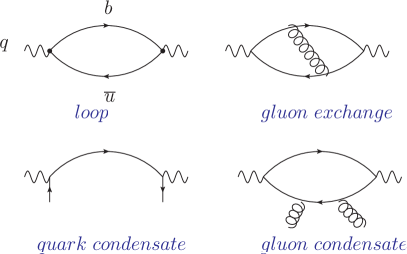
The simple loop diagram and radiative gluon corrections expressed via two- and three-loop diagrams (the latter were calculated in [11]) form the perturbative part of the correlation function $\Pi_{5}(q^{2})$.

Additional diagrams shown in Fig 4 take into account the interactions with QCD vacuum fields. A detailed calculation of the quark condensate diagram shown in Fig. 4 (lower left) can be found e.g., in the review [4]. The gluon condensate diagrams (one of them in Fig 4 (lower right)) are more complicated because they represent a combination of the loop and vacuum insertions. Useful methods to calculate these diagrams are introduced in the review [12]. Technically, one uses Feynman rules of QCD and considers the vacuum quark-antiquark pairs and gluons as external static fields. There are also contributions combining the quark-antiquark and gluon vacuum lines. All condensate diagrams forming the nonperturbative part of $\Pi_{5}(q^{2})$ and calculated at $q^{2}\ll m_{b}^{2}$ contain a short-distance part, formed by the propagating quarks and antiquarks, and a long-distance part approximated by averaged condensate densities. This is how a short-distance quark-antiquark fluctuation “feels” the QCD vacuum, “taking the snapshots” [2] of it.

The result for the correlation $\Pi_{5}(q^{2})$ is an analytical expression in terms of the quark masses $m_{b}$, $m_{u}$, quark-gluon coupling $\alpha_{s}$ and universal QCD condensate densities. Interpreting the calculational procedure as a systematic OPE is another important theoretical aspect. An introduction to the OPE adapted for the correlation functions in the presence of vacuum condensates can be found e.g., in [2, 5]. Formally, one expands the product of two current operators in a series of local operators with growing dimensions, built from quark, antiquark fields and gluon field strength:

$$T\{j_{5}(x)j_{5}^{\dagger}(0)\}=\!\!\!\sum\limits_{d=0,3,4,..}C_{d}(x^{2},m_{b},m_{u},\alpha_{s})O_{d}(0)\,.$$ (11)

Taking vacuum average of the above formula and integrating it over $x$ we recover the correlation function:

$$\Pi_{5}(q^{2})=\int d^{4}x\,e^{iqx}\langle 0|T\{j_{5}(x)j_{5}^{\dagger}(0)\}|0\rangle=\sum\limits_{d=0,3,4,..}\overline{C}_{d}(q^{2},m_{b},m_{u},\alpha_{s})\langle 0|O_{d}|0\rangle\,,$$ (12)

where $\overline{C}_{d}(q^{2},...)=\int d^{4}xe^{iqx}C_{d}(x^{2},...)$. Evidently, only the operators with vacuum quantum numbers (Lorentz-scalar, $C$-, $P$-, $T$-invariant, colourless) contribute to the r.h.s :

$$O_{0}=1,~{}~{}O_{3}=\bar{q}q,~{}~{}O_{4}=G^{a}_{\mu\nu}G^{a\mu\nu},~{}~{}O_{5}=\bar{q}\sigma_{\mu\nu}\frac{\lambda^{a}}{2}G^{a}_{\mu\nu}q,~{}~{}O_{6}=(\bar{q}\Gamma_{r}q)((\bar{q}\Gamma_{r}q),...~{}~{},$$ (13)

where $q=u,d,s$, and $\Gamma_{r}$ are certain combinations of Dirac matrices. The unit operator with $\langle 0|O_{0}|0\rangle=1$ and no fields is added for the sake of uniformity. Its coefficient represents the perturbative part of the correlation function, $\Pi_{5}^{(pert)}(q^{2})=\overline{C}_{0}(q^{2})$. This part is obtained from the loop diagram and gluon radiative corrections and is conveniently represented in the form of a dispersion integral:

$$\Pi_{5}^{(pert)}(q^{2})-\Pi_{5}^{(pert)}(0)-q^{2}\frac{d}{dq^{2}}\Pi_{5}^{(pert)}(0)=(q^{2})^{2}\int\limits_{m_{b}^{2}}^{\infty}\!ds\,\frac{\rho_{5}^{(pert)}(s)}{s^{2}(s-q^{2})}$$ (14)

with the spectral density

$$\rho_{5}^{(pert)}(s)=\frac{1}{\pi}\mbox{Im}\Pi^{(pert)}_{5}(s)=\frac{3m_{b}^{2}}{8\pi^{2}}s\left(1-\frac{m_{b}^{2}}{s}\right)^{2}+O(\alpha_{s})+O(\alpha^{2}_{s})\,.$$ (15)

The two subtractions are needed for the convergence of the integral. Note that for simplicity we neglected the light-quark mass in Eq. (15). The $O(\alpha_{s})$ and $O(\alpha_{s})^{2}$ corrections in this equation are considerably more complicated and can be found in [11, 14] (see also e.g., [13]).

The dominant nonperturbative contribution to the OPE (12) stems from the quark condensate:

$$\Pi^{\langle\bar{q}q\rangle}_{5}(q^{2})=\overline{C}_{3}(q^{2})\langle\bar{q}q\rangle,~{}~{}~{}~{}~{}\mbox{where}~{}~{}\overline{C}_{3}(q^{2})=\frac{-m_{b}^{3}}{m_{b}^{2}-q^{2}}+O(\alpha_{s})\,.$$ (16)

The leading order result for the Wilson coefficient $\overline{C}_{3}(q^{2})$ is obtained from the diagram shown in Fig. 4 (lower left) and a more complicated expression for the $O(\alpha_{s})$ gluon radiative correction can be found in [13]. In the above expression, the separation of short and long distances is visible: the short-distance part is given by a simple $b$-quark propagator with 4-momentum $q$ whereas the quark condensate density represents the long-distance effect. The complete expression for the correlation function in a compact form is:

$$\Pi_{5}^{(OPE)}(q^{2})=\Pi_{5}^{(pert)}(q^{2})+\Pi_{5}^{\langle\bar{q}q\rangle}(q^{2})+\Pi_{5}^{\langle d456\rangle}(q^{2})\,,$$ (17)

where all $d=4,5,6$ effects are collected in one term for brevity. The terms with $d>6$ are usually neglected, provided one keeps the $d=4,5,6$ contribution sufficiently small, due to a proper choice of the variable $q^{2}$.

1.4 Correlation function in terms of hadrons

Having at hand the expression (17) for the correlation function $\Pi_{5}(q^{2})$ valid at $q^{2}\ll m_{b}^{2}$, let us now investigate its relation to hadrons. To visualize the discussion, I consider a hypothetical neutrino-electron elastic scattering via a virtual $W$ boson. One of the possible intermediate states in this process is the $b\bar{u}$ pair emitted from and annihilated into $W$ (in the longitudinal state, to have $J^{P}=0^{-}$) as depicted in Fig. 5. The $b\bar{u}$ fluctuation coincides with the correlation function we are considering.

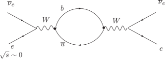
(a)                                                  (b)

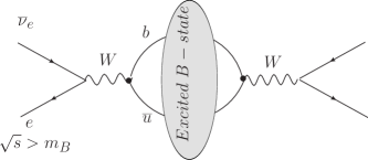
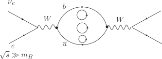
(c)                                                  (d)

Figure 5: Correlation function as a part of the $\bar{\nu}_{e}e$ scattering amplitude at different energies $\sqrt{s}=\sqrt{q^{2}}$.

The c.m. energy of this process is equal to the momentum transfer in the correlation function: $\sqrt{s}=\sqrt{q^{2}}$. In the region $q^{2}\ll m_{b}^{2}$ the intermediate $b\bar{u}$ state (Fig.5(a)) represents a highly virtual heavy-light quark-antiquark pair. We are able to calculate this fluctuation in terms of OPE as already explained. On the other hand, increasing the energy one reaches the domain where real on-shell hadronic states propagate in the intermediate state. At $\sqrt{s}=m_{B}$, the $B$-meson (Fig.5(b)) contributes. This is the lowest possible intermediate hadronic state in this channel, it will show up as a sharp resonance in our hypothetical scattering process. Increasing the energy, one encounters heavier resonances, the radially excited $B$ mesons, with growing total width (Fig.5(c)). These resonances are overlapped with multihadron states with a net $B$ flavor (Fig.5(d)), starting with the two-particle hadronic state $B^{*}\pi$ with the lowest threshold $s=q^{2}=(m_{B^{*}}+m_{\pi})^{2}$. Note that a $B\pi$ state is not allowed by spin-parity conservation. The multihadron state contributions build up the hadronic continuum mixed with excited states. At very large energies, resonances are smeared and multihadron states dominate. We come to conclusion that the correlation function $\Pi_{5}(q^{2})$ in the region $q^{2}>m_{B}^{2}$ describes a complicated overlap of interfering resonant and continuum hadronic states with $B$ meson quantum numbers.

This qualitative picture of emerging intermediate hadronic states reflects the formal spectral representation of $\Pi_{5}(q^{2})$ following from the basic unitarity relation. The imaginary part of the correlation function is equal to the sum of contributions of all possible hadronic states allowed by quantum numbers:

$$\frac{1}{\pi}\mbox{Im}\Pi_{5}(q^{2})=\langle 0|j_{5}|B\rangle\langle B|j_{5}^{\dagger}|0\rangle\delta(m_{B}^{2}-q^{2})+\rho^{h}_{5}(s)\theta(s-(m_{B^{*}}+m_{\pi})^{2})\,,$$ (18)

where we isolated the ground-state $B$ meson contribution and introduce a shorthand notation for the spectral density of excited (resonance and multiparticle) states, schematically:

$$\rho^{h}_{5}(s)=\sum_{B_{exc}}\langle 0|j_{5}|B_{exc}\rangle\langle B_{exc}|j_{5}^{\dagger}|0\rangle$$ (19)

where the sum includes the integration over phase space and sum over polarizations.

The next important step is to employ the analyticity of the function $\Pi(q^{2})$ which, according to the unitarity relation (18) has singularities – poles (cuts) related to resonances (multiparticle thresholds) – on the real positive axis of the complex $q^{2}$ plane. The Cauchy theorem leads to the dispersion relation between $\Pi_{5}(q^{2})$ and its imaginary part integrated over positive $s\geq m_{B}^{2}$:

$$\Pi_{5}(q^{2})=\frac{1}{\pi}\int\limits_{m_{B}^{2}}^{\infty}ds\frac{\mbox{Im}\Pi_{5}(s)}{s-q^{2}-i\epsilon}\,,$$ (20)

where the subtraction terms are hereafter neglected for simplicity. Importantly, this relation is valid at any $q^{2}$. We will apply it at $q^{2}\ll m_{b}^{2}$ where the correlation function represents a short-lived $b\bar{u}$ -fluctuation calculable in terms of OPE, so that l.h.s. in the above dispersion relation can be approximated by $\Pi_{5}^{(OPE)}(q^{2})$ given by Eq. (17). Hence, we obtain a remarkable opportunity to relate the correlation function calculated in QCD to a sum/integral containing hadronic parameters, including the $B$-meson mass and decay constant.

1.5 Deriving the sum rule for $f_{B}^{2}$

Substituting Eq. (18) in the dispersion relation (20) and expressing the hadronic matrix element via $f_{B}$, we obtain at $q^{2}\ll m_{b}^{2}$:

$$\Pi_{5}(q^{2})=\frac{f_{B}^{2}m_{B}^{4}}{m_{B}^{2}-q^{2}}+\int\limits_{s_{h}}^{\infty}ds\frac{\rho^{h}(s)}{s-q^{2}}\simeq\Pi^{(OPE)}_{5}(q^{2})\,.$$ (21)

where $s_{h}=(m_{B^{*}}+m_{\pi})^{2}$ is the lowest threshold of the excited $B$ states.

Let us now employ another important feature of the correlation function. In the deep spacelike region $q^{2}\to-\infty$ the power suppressed condensate terms in Eq. (17) vanish and the correlation function coincides with the perturbative part of OPE:

$$\Pi_{5}(q^{2}\to-\infty)=\Pi^{(OPE)}_{5}(q^{2}\to-\infty)=\Pi^{(pert)}_{5}(q^{2}\to-\infty)\,,$$ (22)

dominated by the simple loop diagram.

It is convenient to express the perturbative part of the OPE in a form of dispersion relation. In this case the imaginary part starts at the $b\bar{u}$-quark pair threshold and is equal to the spectral density of the loop diagrams presented in Eq. (15):

$$\Pi^{(pert)}(q^{2})=\frac{1}{\pi}\int\limits_{m_{b}^{2}}^{\infty}ds\frac{\mbox{Im}\Pi^{(pert)}_{5}(s)}{s-q^{2}}\,,$$ (23)

where we again neglect the subtractions and put $m_{u}\to 0$.

To fulfill the asymptotic condition (22), the spectral functions entering the hadronic and OPE (perturbative) dispersion relations should be equal at sufficiently large $s$:

$$\rho^{h}(s)\simeq\frac{1}{\pi}\mbox{Im}\Pi_{5}^{(pert)}(s),$$ (24)

This approximation is called local quark-hadron duality. It suffices to use a weaker condition, approximately equating the integrals of the hadronic and perturbative spectral densities over the large $s$ region:

$$\int\limits_{s_{h}}^{\infty}ds\frac{\rho^{h}(s)}{s-q^{2}}\simeq\frac{1}{\pi}\int\limits_{s_{0}}^{\infty}ds\frac{\mbox{Im}\Pi^{(pert)}_{5}(s)}{s-q^{2}}\,,$$ (25)

where an effective threshold $s_{0}$ is introduced. Returning to the hadronic dispersion relation (21), we use Eq. (25) to replace the integral over excited $B$ states in l.h.s., and use the OPE (17) in r.h.s., with the perturbative part replaced by its dispersion representation. The resulting relation:

$$\frac{f_{B}^{2}m_{B}^{4}}{m_{B}^{2}-q^{2}}+\frac{1}{\pi}\int\limits^{\infty}_{s_{0}}ds\frac{\mbox{Im}\Pi^{(pert)}_{5}(s)}{s-q^{2}}=\frac{1}{\pi}\int\limits^{\infty}_{m_{b}^{2}}ds\frac{\mbox{Im}\Pi^{(pert)}_{5}(s)}{s-q^{2}}+\Pi_{5}^{\langle\bar{q}q\rangle}(q^{2})+\Pi_{5}^{\langle d456\rangle}(q^{2})\,,$$ (26)

allows one to subtract the approximately equal integrals from both sides yielding an analytical relation for the decay constant:

$$\frac{f_{B}^{2}m_{B}^{4}}{m_{B}^{2}-q^{2}}=\frac{1}{\pi}\int\limits^{s_{0}}_{m_{b}^{2}}ds\frac{\mbox{Im}\Pi^{(pert)}_{5}(s)}{s-q^{2}}+\Pi_{5}^{\langle\bar{q}q\rangle}(q^{2})+\Pi_{5}^{\langle d456\rangle}(q^{2})\,.$$ (27)

A substantial improvement of this relation is further achieved with the help of the Borel transformation defined as:

$$\Pi_{5}(M^{2})\equiv{\cal B}_{M^{2}}\Pi_{5}(q^{2})=\lim_{\stackrel{{\scriptstyle-q^{2},n\to\infty}}{{-q^{2}/n=M^{2}}}}\frac{(-q^{2})^{(n+1)}}{n!}\left(\frac{d}{dq^{2}}\right)^{n}\Pi_{5}(q^{2})~{},$$ (28)

so that ${\cal B}_{M^{2}}(\frac{1}{m^{2}-q^{2}})=\exp(-m^{2}/M^{2})$.

The resulting QCD sum rule for $f_{B}^{2}$ obtained from Eq. (27) after this transformation reads:

$$f_{B}^{2}m_{B}^{4}e^{-m_{B}^{2}/M^{2}}=\int\limits_{m_{b}^{2}}^{s_{0}}dse^{-s/M^{2}}\mbox{Im}\Pi_{5}^{(pert)}(s,m_{b},m_{u},\alpha_{s})+\Pi_{5}^{\langle\bar{q}q\rangle}(M^{2})+\Pi_{5}^{\langle d456\rangle}(M^{2})\,.$$ (29)

Note that the Borel transformation suppresses the higher-state contributions to the hadronic sum above $s_{0}$ so that the above sum rule is less sensitive to the accuracy of the quark-hadron duality approximation (25). Everything is ready to calculate the decay constant of $B$ meson numerically.

1.6 Input parameters and results

In the sum rule (29) one has to choose an optimal interval of the Borel parameter. The lower boundary for $M^{2}$ is controlled by the OPE convergence, e.g., we demand that the $d=4,5,6$ terms are sufficiently small with respect to the quark condensate term. The upper boundary for $M^{2}$ is adopted from the condition that the contribution of excited states subtracted from the sum rules remains subdominant. Furthermore, a standard way to fix the effective parameter $s_{0}$ is to fit the sum rule to the measured mass of $B$-meson by differentiating both parts of Eq. (29) in $-(1/M^{2})$ and dividing the result by the initial sum rule, so that $f_{B}^{2}$ cancels, and one obtains a relation for $m_{B}^{2}$.

One of the advantages of the sum rule method is its flexibility: replacing quark flavours in the correlation function, e.g., $b\to c$ or $\bar{u}\to\bar{s}$ provides an access to the decay constants of $D$ or $B_{s}$ mesons.

Decay constant Lattice QCD [ref.] QCD sum rules [13] 196.9 $\pm$ 9.1 [20] $f_{B}$[MeV] $207^{+17}_{-9}$ 186 $\pm$ 4 [21] 242.0 $\pm$ 10.0 [20] $f_{B_{s}}$[MeV] $242^{+17}_{-12}$ 224 $\pm$ 5 [21] 1.229$\pm$ 0.026 [20] $f_{B_{s}}/f_{B}$ $1.17^{+0.04}_{-0.03}$ 1.205$\pm$ 0.007 [21] 218.9 $\pm$ 11.3 [20] $f_{D}$[MeV] $201^{+12}_{-13}$ 213 $\pm$ 4 [22] 260.1 $\pm$ 10.8 [20] $f_{D_{s}}$[MeV] $238^{+13}_{-23}$ 248.0 $\pm$ 2.5 [22] 1.188$\pm$ 0.025 [20] $f_{D_{s}}/f_{D}$ $1.15^{+0.04}_{-0.05}$ 1.164$\pm$ 0.018 [22]

Table 1: Decay constants of heavy-light mesons calculated with different methods.

Nonzero strange quark mass and a difference in condensate densities, $\langle\bar{s}s\rangle\neq\langle\bar{u}u\rangle$, generate the $SU(3)_{flavour}$ symmetry violation.

The universal input parameters needed for the numerical analysis of the sum rules include the quark masses, quark-gluon coupling and the vacuum condensate densities. Since the calculation is done at short distances, the natural choice for quark masses is the $\overline{MS}$ scheme. The sum rule is quite sensitive to the $b$-quark mass, hence to have a reliable estimate of $f_{B}$ one needs an independent and accurate determination of $m_{b}$. This task was fulfilled by considering quarkonium sum rules, where the correlation function of two $\bar{Q}\gamma_{\mu}Q$ currents ($Q=b,c$) is calculated in QCD. The accuracy of this calculation [15] has reached $O(\alpha_{s}^{3})$ in the perturbative part. The hadronic representation of this correlation function is largely fixed from experiment [16] and consists of $J^{PC}=1^{--}$ heavy quarkonia levels, their decay constants measured in $e^{+}e^{-}\to\Upsilon,\Upsilon(2S),....$ or $e^{+}e^{-}\to J/\psi,\psi(2S),....$. Hence, the quarkonium sum rules can be used to extract the heavy quark masses. The most recent results of these determinations [15, 17], expressed in $\overline{MS}$ scheme are very close to the PDG averages: $\bar{m}_{b}(\bar{m}_{b})=(4.18\pm 0.03)\,\mbox{GeV}$, $\bar{m}_{c}(\bar{m}_{c})=(1.275\pm 0.025)\,\mbox{GeV}$ [16]. In the same way, employing QCD sum rules for strange meson pseudoscalar and scalar channels [18] one determines $m_{s}$ consistent with $m_{s}(\mu=2\,\mbox{GeV})=(95\pm 10)\,\mbox{MeV}$[16]. Combining $m_{s}$ with ChPT relations [19] one finds the quark condensate density $\langle\bar{q}q\rangle(\mbox{2 GeV})=-(277^{+12}_{-10}~{}\mbox{MeV})^{3}$. Condensate densities with $d>3$ entering the subleading power corrections in OPE are mainly taken from the review [9]. The recent determinations of the $B$ and $D$ decay constants in Table 1 are taken from [13] where one can also find a detailed discussion of numerical procedure and formulae for OPE, as well as references to other important papers on the subject of this lecture.

2 ​​​​​​. Lecture: $B\to\pi$ form factors and light-cone sum rules

In this lecture more complicated hadronic matrix elements – the form factors of heavy-to-light transitions are considered. The best studied among them are the $B\to\pi$ transition form factors relevant for $B\to\pi\ell\nu_{\ell}$ semileptonic decay. I will explain how the QCD sum rule method was modified to calculate these and other hadronic form factors.

2.1 $B\to\pi\ell\nu_{\ell}$ decay and form factors

Figure 6: Schematic view of $B\to\pi\ell\nu_{\ell}$ decay

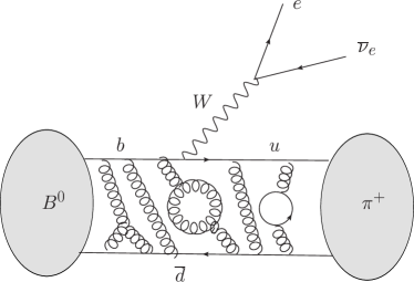
The exclusive semileptonic decay $\bar{B}^{0}\to\pi^{+}\ell\bar{\nu}_{\ell}$ shown in Fig. 6 proceeds via weak $b\to u$ transition with a squared momentum transfer $q^{2}$ to the leptonic pair varying within the interval $0<q^{2}<(m_{B}-m_{\pi})^{2}\sim 26~{}\mbox{GeV}^{2}$ (here we neglect the lepton mass).

The form factors $f^{+}_{B\pi}(q^{2})$ and $f^{0}_{B\pi}(q^{2})$ are invariant functions of $q^{2}$ parameterizing the hadronic matrix element of this decay:

$$\langle\pi^{+}(p)|\bar{u}\gamma_{\mu}b|\bar{B}^{0}(p+q)\rangle=f^{+}_{B\pi}(q^{2})\Big{[}2p_{\mu}+\big{(}1-\frac{m_{B}^{2}-m_{\pi}^{2}}{q^{2}}\big{)}q_{\mu}\Big{]}+f^{0}_{B\pi}(q^{2})\frac{m_{B}^{2}-m_{\pi}^{2}}{q^{2}}q_{\mu},$$ (30)

where $p+q$ and $p$ are the four-momenta of $B$ and $\pi$, respectively. Similar to the $B$ decay constant, the $B\to\pi$ form factors have to be calculated in QCD. This is a challenging problem because not only the initial $B$ meson but also the final pion is involved in the hadronic matrix element. In what follows, we consider the region of small $q^{2}$, in which case the pion has a large recoil in the $B$ meson rest system, with the momentum $p_{\pi}\equiv|\vec{p}\,|\sim m_{B}/2$ at $q^{2}=0$.

Analyzing the $B\to\pi$ form factors from the point of view of QCD, one expects a certain perturbative contribution corresponding to an energetic virtual gluon exchange between the quarks participating in the weak transition and the spectator quark. This “hard scattering” mechanism boosts the spectator quark in $B$ meson and provides a natural configuration for the final pion with symmetric collinear quark and antiquark. On the other hand one has to take into account also the “end-point” mechanism where the pion is formed from an asymmetric quark-antiquark pair. This part of the form factor is dominated by soft nonperturbative gluons. The proportion of the hard scattering and soft end-point contributions to the hadronic form factors is a long-standing problem. It can only be addressed within a calculational method that allows one to take into account both contributions.

An accurate determination of the $B\to\pi$ form factors is important for quark flavour physics because the semileptonic decay $B\to\pi\ell\nu_{\ell}$ is an excellent source of the CKM parameter $|V_{ub}|$. In fact, one practically needs only the vector form factor $f^{+}_{B\pi}$ for this purpose, because in the partial width the contribution of the form factor $f^{0}_{B\pi}$ is suppressed by the lepton mass:

$$\frac{1}{\tau_{B^{0}}}\frac{dBR(\bar{B}^{0}\to\pi^{+}l^{-}\nu)}{dq^{2}}=\frac{G_{F}^{2}|V_{ub}|^{2}}{24\pi^{3}}p_{\pi}^{3}|f^{+}_{B\pi}(q^{2})|^{2}+O(m_{l}^{2})\,.$$ (31)

Importantly, in lattice QCD the $B\to\pi$ form factors are currently accessible at comparatively large $q^{2}\geq 15$ GeV². In this region the phase space in the decay width (31) is suppressed by small $p_{\pi}$. The calculation of the form factors at small $q^{2}$ (large recoil of the pion) discussed below, complements the lattice QCD results in a kinematically dominant region.

2.2 Vacuum-to-pion correlation function

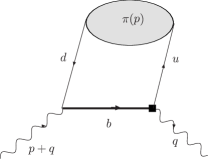
The method of light-cone sum rules (LCSR) developed in [23, 24] is used to calculate the $B\to\pi$ form factors at large hadronic recoil. In this approach, the correlation function itself is an amplitude of the vacuum-to-hadron transition :

$$F_{\lambda}(q,p)=i\int d^{4}x~{}e^{iqx}\langle\pi(p)\mid T\{\bar{u}(x)\gamma_{\lambda}b(x),j^{\dagger}_{5}(0)\}\mid 0\rangle$$

$$=F(q^{2},(p+q)^{2})p_{\mu}+\tilde{F}(q^{2},(p+q)^{2})q_{\mu}\,,$$ (32)

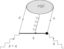
containing the product of the weak $b\to u$ and $j_{5}=m_{b}\,\bar{b}i\gamma_{5}d$ currents. The latter was also used in the two-point correlation function for $f_{B}$. In what follows, only the invariant amplitude $F$ is essential, depending on the two independent kinematical variables: $q^{2}$ , the squared momentum transfer in the weak $b\to u$ transition, and $(p+q)^{2}$, the square of the 4-momentum flowing into the current $j_{5}$. The correlation function (32) allows for a systematic QCD calculation in the specific region: $q^{2},(p+q)^{2}\ll m_{b}^{2}$ where the $b$ quark is a highly-virtual object. In this region of external momenta the $x$ integral in the correlation function is dominated by small $x^{2}\sim 1/m_{b}^{2}$, near the light-cone $x^{2}\sim 0$. The leading order diagram for the correlation function is shown in Fig. 7(a). It consists of the free $b$-quark propagator convoluted with the matrix element of light quark and antiquark operators sandwiched between the vacuum and on-shell pion state. The perturbative gluon corrections to the leading order diagram are shown in Fig. 8. The diagram in Fig. 7(b) takes into account the emission of a soft (low-virtuality) gluon emitted from the $b$ quark. The corresponding vacuum-pion matrix element involves light quark-antiquark and gluon fields.

A schematic expression for the correlation function (32) decomposed near the light-cone can be written as:

(a)                                             (b)

Figure 7: Diagrams corresponding to the correlation function (32): leading order (a) and soft gluon emission forming the 3-particle $B$ meson DA (b).

Figure 8: Gluon radiative corrections to the correlation function (32).

$$\!\!\!\!\!F(q,p)=i\int d^{4}x\,e^{iqx}\Bigg{\{}\left[S^{0}(x^{2},m_{b}^{2})+\alpha_{s}S^{1}(x^{2},m_{b}^{2})\right]\langle\pi(p)\mid\bar{u}(x)\Gamma d(0)\!\mid\!0\rangle$$

$$+\int_{0}^{1}dv~{}\tilde{S}(x^{2},m_{b}^{2},v)\langle\pi(p)\mid\bar{u}(x)G(vx)\tilde{\Gamma}d(0)\}\mid 0\rangle\Bigg{\}}+...$$ (33)

where $S_{0}$ , $S_{1}$ and $\tilde{S}$ are the perturbative parts of the amplitudes, involving $b$-quark propagators. They are convoluted with the vacuum-pion matrix elements, taken near $x^{2}=0$, where $\Gamma,\tilde{\Gamma}$ are generic Dirac-matrix structures and the Lorentz-indices are omitted for simplicity.

The vacuum-pion matrix elements in Eq. (33) are nonperturbative but universal objects. They absorb all long-distance effects in the correlation function. The expansion in Eq.(33) goes over $\alpha_{s}$ and powers of $x^{2}$, which in the momentum space translates into an expansion in $\alpha_{s}(\mu)$ and the powers of $1/\mu$. Here $\mu\sim\sqrt{\chi m_{b}}$ , with $\chi$ being an intermediate scale, $\Lambda_{QCD}\ll\chi<m_{b}$. In particular, in (33) the quark-antiquark gluon part has a power suppression with respect to the leading order part. Hence, the expansion (33) can safely be truncated. I skip a more formal and systematic description of this expansion based on the twist $t$ (dimension minus Lorentz-spin) of the light quark-antiquark operators entering the vacuum-pion matrix elements (see, e.g., [5] for an introductory explanation).

The main nonperturbative object determining the leading-order answer for the light-cone expanded correlation function (33) is the vacuum-pion matrix element

$$\langle\pi(q)|\bar{u}(x)[x,0]\gamma_{\mu}\gamma_{5}d(0)|0\rangle_{x^{2}=0}=-iq_{\mu}f_{\pi}\int_{0}^{1}du\,e^{iuqx}\varphi_{\pi}(u)+O(x^{2})~{},$$ (34)

where the factor $[x,0]=exp[ig_{s}\int_{0}^{1}dtx_{\mu}A^{a\mu}(tx)\lambda^{a}/2]$ is added to secure gauge invariance. The above matrix element is normalized to the pion decay constant, which becomes evident if one puts $x\to 0$ and takes into account that the function $\varphi_{\pi}(u)$ is normalized to unit. This and similar functions parameterizing vacuum-pion matrix elements play the central role in the LCSR approach and replace the vacuum condensates. They are called light-cone distribution amplitudes (DA’s) of the pion. Physically, DA’s correspond to various Fock components of the pion and the variable $u$ in the two-particle DA (34) denotes the share of the pion momentum carried by one of the constituents.

Inserting in Eq. (33) the vacuum-pion matrix elements expressed in terms of DA’s and integrating over $x$, one obtains the OPE result for the invariant amplitude defined in (32) in the following generic form:

$$F^{(OPE)}(q^{2},(p\!+\!q)^{2})=\sum\limits_{t=2,3,4,..}\int du~{}T^{(t)}(q^{2},(p\!+\!q)^{2},m_{b}^{2},\alpha_{s},u,\mu)\,\varphi^{(t)}_{\pi}(u,\mu)\,,$$ (35)

where the summation goes over the growing twist, and the twist-2 part contains the DA defined in Eq. (34). The perturbative hard-scattering amplitudes $T^{(t)}$ stemming from the $b$-quark propagators and perturbative loops are process-dependent whereas the pion DA’s are universal. One can analyse DA’s using the light-cone OPE for other processes, not even involving heavy quarks, like e.g., the pion electromagnetic form factor at spacelike momentum transfers or the photon-pion transition form factor (see e.g. [5]). Within the currently achieved accuracy, the light-cone OPE (35) includes the twist 2,3,4 quark-antiquark and quark-antiquark-gluon DA’s [25], and the hard-scattering amplitudes for twist 2,3 parts are calculated up to NLO, in $O(\alpha_{s})$ [26, 27, 28, 29]. Recently, the $O(\alpha_{s}^{2})$ correction to the twist-2 part was also calculated [30].

2.3 What do we know about the light-cone DA’s

Before applying them in LCSR’s, the pion DA’s were already introduced in the context of the hard-scattering mechanism for the pion e.m. form factor at large momentum transfer [31, 32]. A convenient expansion in Gegenbauer polynomials was defined

$$\varphi_{\pi}(u,\mu)=6u(1-u)\left[1+\sum\limits_{n=2,4,..}a_{n}^{\pi}(\mu)C_{n}^{3/2}(2u-1)\right],$$ (36)

with logarithmic evolution of its coefficients (Gegenbauer moments):

$$a_{2n}^{\pi}(\mu)\sim[\ln(\mu/\Lambda_{QCD})]^{-\gamma_{2n}}\,,$$ (37)

vanishing at asymptotically large scale $\mu\to\infty$. The input values of Gegenbauer moments at low scale, $a_{2,4,6,...}^{\pi}(\mu\sim\mbox{ 1 GeV})$ are determined from different sources: matching experimentally measured pion form factors to LCSR’s , calculating $a_{2}$ from two-point QCD sum rules and in lattice QCD. Recent determinations lie within the intervals: $a_{2}^{\pi}=0.25\pm 0.15$,  $a^{\pi}_{2}+a_{4}^{\pi}=0.1\pm 0.1$, if one neglects the higher coefficients. The remaining parameters of twist 3,4 DA’s are mainly determined from dedicated two-point sum rules [33].

2.4 LCSR for $B\to\pi$ form factors

After obtaining the OPE expression for the amplitude $F((p+q)^{2},q^{2})$, the derivation of LCSR follows the same strategy as in the case of two-point sum rule. The hadronic dispersion relation for $F((p+q)^{2},q^{2})$ in the variable $(p+q)^{2}$ and at fixed small $q^{2}$ is used. The dispersion relation contains a pole term with intermediate $B$ meson and a hadronic sum over excited and multihadron states with $B$ quantum numbers. Matching the OPE with this dispersion relation, we obtain

$$F^{(OPE)}((p+q)^{2},q^{2})=\frac{2m_{B}^{2}f_{B}f_{B\pi}^{+}(q^{2})}{m_{B}^{2}-(p+q)^{2}}+\frac{1}{\pi}\int\limits_{s_{0}}^{\infty}ds\frac{\mbox{Im}F^{(OPE)}(s,q^{2})}{s-(p+q)^{2}}\,,$$ (38)

where the residue of the $B$-meson pole term contains the product of matrix elements $\langle\pi\!\mid\!\bar{u}\gamma_{\lambda}b\!\mid\!B\rangle$ and $\langle B\!\mid j^{\dagger}_{5}\mid\!0\rangle$, yielding the product of the form factor $f_{B\pi}^{+}(q^{2})$ and the decay constant $f_{B}$. For the latter, the result obtained from the two-point sum rule discussed in the previous lecture can be used. Furthermore, on r.h.s. of (38) we also use the quark-hadron duality approximation, replacing the integral over excited states by the integral over the spectral density of the OPE result with an effective threshold $s_{0}$. Subtracting the integrals from $s_{0}$ to $\infty$ from both sides of the above relation and performing the Borel transformation we finally obtain the desired LCSR for the form factor:

$$f_{B}f_{B\pi}^{+}(q^{2})=\frac{1}{2\pi m_{B}^{2}}\int\limits_{m_{b}^{2}}^{s_{0}}ds~{}\mbox{Im}F^{(OPE)}(s,q^{2})e^{(m_{B}^{2}-s)/M^{2}}\,.$$ (39)

The inputs include the $b$-quark mass $\overline{m}_{b}$, $\alpha_{s}$, and the set of pion DA’s $\varphi_{\pi}^{(t)}(u)$, t=2,3,4. The resulting numerical interval for the form factor is formed by the uncertainties due to variation of the input and of $M^{2}$ within the interval where one can trust OPE and where simultaneously the contribution of excited states remains subdominant. A very detailed numerical analysis of this sum rule can be found in [29, 34]. The effective threshold can be controlled by the $m^{2}_{B}$ calculation from LCSR. The LCSR for the scalar $B\to\pi$ form factor $f^{0}_{B\pi}$ is obtained employing the second invariant amplitude in the correlation function (32).

Let me emphasize that the method discussed here employs a finite $b$-quark mass. At the same time LCSRs allow for a systematic transition to the infinite heavy-quark mass. This limit described in detail, e.g., in the reviews [4, 6], reproduces the heavy-mass scaling of the form factor at large hadronic recoil

$$f^{+}_{B\pi}(q^{2}=0)\sim 1/m_{b}^{3/2}\,,$$ (40)

first predicted in [24]. Another important feature of LCSRs is that they contain both soft end-point and hard-scattering contributions to the form factor. The hard-scattering part is contained in the $O(\alpha_{s})$ contributions to LCSR, described by the diagrams with perturbative gluon exchanges. The soft end-point mechanism originates from the part of OPE that do not contain gluon exchanges, and is dominated by the leading order diagram. It is therefore not surprising that the hard scattering part is suppressed, supporting the dominance of the end-point mechanism for the form factor.

         

Figure 9: LCSR results [34] for $B\to\pi$ form factors, extrapolated to $q^{2}>12$ GeV² in comparison with the lattice QCD predictions [35]

.

In Fig. 9 the recent predictions [34] of LCSR for both $B\to\pi$ form factors are shown in comparison with the lattice QCD results [35]. The sum rules are used at $q^{2}<q^{2}_{max}\simeq 12$ GeV² and the results are then extrapolated to larger momentum transfers with a certain analytical parametrization of the form factors [36] as explained in detail in [34]. Finally, the LCSR results were used to evaluate an integral over the weighted form factor squared, which, as follows from (31), is related to the integral over the partial width:

$$\frac{G_{F}^{2}}{24\pi^{3}}\int\limits_{0}^{q_{max}^{2}}dq^{2}p_{\pi}^{3}|f_{B\pi}^{+}(q^{2})|^{2}=\frac{1}{|V_{ub}|^{2}\tau_{B^{0}}}\int\limits_{0}^{q_{max}^{2}}dq^{2}\frac{d{\cal B}(B\to\pi\ell\nu_{\ell})}{dq^{2}}\,,$$ (41)

This relation together with the measurements of the integrated partial width of $B\to\pi\ell\nu_{\ell}$ were used to extract $|V_{ub}|$.

Simple replacements $b\to c$ and the adjustment of light quark flavours in the underlying correlation function (32) allows to obtain the LCSR’s for $D\to\pi,K$ form factors [37] employing the same OPE diagrams. In this case, only a narrow region above $q^{2}=0$ is accessible with LCSR’s. The $SU(3)_{flavour}$ symmetry violation is encoded in the Gegenbauer moments of the kaon $a_{n}^{K}$ , in particular, the odd moments with $n=1,3,...$ have to be added in the expansion (36). The results for the form factors were used in [37] to extract $V_{cs}$ and $V_{cd}$ from the data on $D\to\pi(K)\ell\nu_{\ell}$ decays.

2.5 Alternative sum rules with $B$-meson DA’s

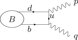
The positions of the $B$-meson interpolating current and pion in the correlation function (32) can be exchanged, introducing a new, vacuum-to-$B$ correlation function, in which the $B$ meson is represented by an on-shell state and the pion is replaced by an interpolating quark current, as shown in Fig. 10. Here $q$ is the momentum transfer in the weak $b\to u$ transition current and $p$ is the external momentum of the light-meson interpolating current, whereas $p_{B}=p+q$ with $p_{B}^{2}=m_{B}^{2}$ is the $B$-meson momentum.

This approach was initiated in [38] (see also [39]). Its main advantage is an easy extension to other light hadrons, also the non-stable ones. It is relatively easy to obtain LCSRs for the $B$-meson transition form factors to light vector, scalar or axial mesons, by simply varying the quantum numbers of the interpolating current and adjusting the quark-hadron duality ansatz.

Figure 10: Correlation function with B-meson DA’s

The description in terms of the light-cone OPE is done in the framework of heavy-quark effective theory (HQET). The 4-momentum of $b$ -quark and $B$ meson are represented as a sum of the static component and residual momentum: e.g, $p_{B}=p+q=m_{b}v+k$ where $v$ is the velocity 4-vector. After the transition to HQET the vacuum-to-$B$ correlation function is independent of the scale $m_{b}$. In this effective theory the following definition [41, 40] of the vacuum-$B$ matrix element is used

$$\langle 0|\bar{q}_{2\alpha}(x)[x,0]h_{v\beta}(0)|\bar{B}_{v}\rangle$$

$$=-\frac{if_{B}m_{B}}{4}\int\limits_{0}^{\infty}d\omega e^{-i\omega v\cdot x}\left[(1+/\!\!\!v)\left\{\phi^{B}_{+}(\omega)-\frac{\phi_{+}^{B}(\omega)-\phi_{-}^{B}(\omega)}{2v\cdot x}/\!\!\!x\right\}\gamma_{5}\right]_{\beta\alpha}\,,$$ (42)

where $h_{v\beta}$ is the effective field, $\alpha,\beta$ are Dirac indices. The functions $\phi_{\pm}^{B}(\omega)$ are the $B$-meson two-particle DA’s and $\omega$ is the light-quark momentum fraction which formally (in the infinite heavy quark limit) varies up to $\omega=\infty$, however, in all realistic models is limited by $\omega\sim\bar{\Lambda}$ where $\bar{\Lambda}$ is the mass difference introduced in Eq. (6). More details on $B$-meson DA’s can be found in the review [42]. These DA’s were used earlier in the context of factorization approach to the heavy-light form factors in HQET [40]. In addition, the diagram with soft gluon emitted from $u$ quark in the correlation function was taken into account, generating the three-particle DA’s. Their detailed discussion can be found in the second paper in [38].

The rest of LCSR derivation follows the same way as in the case of pion DA’s. The OPE in terms of $B$-meson DA’s is matched to the dispersion relation in the variable $p^{2}$ which is the invariant momentum squared of the light-meson interpolating current. The accuracy of resulting LCSR’s for $B\to\pi,K,\rho,K^{*}$ form factors obtained in [38] is still lower than for the conventional sum rules. One reason is that the key nonperturbative input parameter, the inverse moment: $\frac{1}{\lambda_{B}(\mu)}=\int_{0}^{\infty}d\omega\frac{\phi_{+}^{B}(\omega,\mu)}{\omega}$ is not yet accurately determined. Two-point QCD sum rules in HQET predict $\lambda_{B}(1~{}\mbox{GeV})=460\pm 110~{}\mbox{MeV}$ [43]. This parameter is accessible in the photoleptonic’ $B\to\gamma\ell\nu_{\ell}$ decay (for recent analyses see [44] and [45]). Another reason is that the radiative gluon corrections to the correlation function in Fig. 10 are still missing. Therefore, the LCSR’s with B-meson DA’s have a room for improvement. Finally, let me quote another important application of this method [46] to $B\to D^{(*)}$ form factors. The sum rules were obtained from the same correlation function as in Fig. 10 replacing the light quark in the correlation function by a $c$ quark - another manifestation of the flexibility and universality of the method.

2.6 Heavy baryon form factors and $\Lambda_{b}\to p\,\ell\nu_{\ell}$

The LCSR method for B-meson form factors was also extended to the heavy baryon form factors. In particular, let me briefly outline the recent calculation [47] of the $\Lambda_{b}\to p$ form factors employing the following vacuum-to-nucleon correlation function:

$$\Pi_{\mu(5)}(P,q)=i\int d^{4}z\ e^{iq\cdot z}\langle 0|T\left\{\eta_{\Lambda_{b}}(0),\bar{b}(z)\gamma_{\mu}(\gamma_{5})u(z)\right\}|N(P)\rangle\,.$$ (43)

Figure 11: Diagrammatic representation of the correlation function with nucleon DA’s used to derive LCSR’s for heavy-to-light baryon form factors.

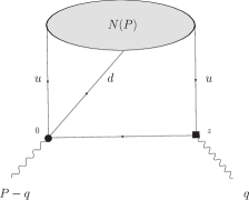
Here the three-quark heavy-light current operator $\eta_{\Lambda_{b}}$ with quantum numbers of $\Lambda_{b}$ has a nonvanishing matrix element $\langle\Lambda_{b}\mid\eta_{\Lambda_{b}}\mid 0\rangle\neq 0$. It is traditionally called the $\Lambda_{b}$ “decay constant”, although literally an annihilation of $\Lambda_{b}$ would violate the baryon number conservation and is absent in SM. Nevertheless, in QCD nothing prevents from introducing the auxiliary operator $\eta_{\Lambda_{b}}$ as an external source of $b$-quark baryonic states. As opposed to the meson case, one has a multiple choice for constructing the three-quark currents. In [47] two different operators were used:

$$\eta^{({\cal P})}_{\Lambda_{b}}=\left(u\,C\,\gamma_{5}\,d\right)b,~{}~{}\eta^{({\cal A})}_{\Lambda_{b}}=\left(u\,C\,\gamma_{5}\gamma_{\lambda}\,d\right)\gamma^{\lambda}\,b\,,$$ (44)

and the difference between the results for the form factors was considered as a part of the “systematic” uncertainty.

The diagram for the correlation function in LO is shown in Fig. 11, with the on-shell nucleon, carrying the 4-momentum $P$ ($P^{2}=m_{N}^{2}$) and with the horizontal line denoting the virtual $b$-quark. The approximation of the free $b$-quark propagation is valid in the kinematical region $q^{2}\ll m_{b}^{2}$ , $(P-q)^{2}\ll m_{b}^{2}$, where the integral over $z$ in Eq. (43) is dominated by small intervals near the light-cone, $z^{2}\sim 0$.

Contracting the virtual $b$-quark fields in Eq. (43), we recover new nonperturbative objects: the nucleon DA’s. Their definitions and properties were worked out in [48], where also the LCSR’s for nucleon electromagnetic form factors were obtained. The latter sum rules are described by the same diagram of Fig. 11 with a light $u,d$ quark in the horizontal line. The definition of DA’s is schematically given by the following decomposition of the vacuum-nucleon matrix element:

$$\langle 0|\epsilon^{ijk}u_{\alpha}^{i}(0)u_{\beta}^{j}(z)d_{\gamma}^{k}(0)|N(P)\rangle=\sum_{t}\mathcal{S}^{(t)}_{\alpha\beta\gamma}\times\int dx_{1}dx_{2}dx_{3}\delta(1-\sum_{i=1}^{3}x_{i})e^{-ix_{2}P\cdot z}F_{t}(x_{i})\,,$$ (45)

where the expansion goes over twist $t=3,4,5,6$ of light-quark operators and contains 27 DA’s $F_{t}(x_{i})$ depending on the shares $x_{1,2,3}$ of the nucleon momentum.

The hadronic dispersion relation for the correlation function (43) aimed at isolating the ground-state $\Lambda_{b}$-pole contribution also has its peculiarities. The baryonic quark currents not only interpolate the ground states but also their counterparts with the opposite $P$ parity. In our case, the $\Lambda_{b}^{*}$ baryon with $J^{P}=1/2^{-}$ located at $m_{\Lambda^{*}_{b}}\simeq m_{\Lambda_{b}}+(200\div 300)$ MeV, should also be counted as a ground state in the hadronic spectrum. Therefore we have to include this state in the resulting dispersion relation separately from the excited states:

$$\Pi_{\mu(5)}(P,q)=\frac{\langle 0|\eta_{\Lambda_{b}}|\Lambda_{b}\rangle\langle\Lambda_{b}|\bar{b}\gamma_{\mu}(\gamma_{5})u|N\rangle}{m_{\Lambda_{b}}^{2}-(P-q)^{2}}+\frac{\langle 0|\eta_{\Lambda_{b}}|\Lambda^{*}_{b}\rangle\langle\Lambda^{*}_{b}|\bar{b}\gamma_{\mu}(\gamma_{5})u|N\rangle}{m_{\Lambda_{b}^{*}}^{2}-(P-q)^{2}}+\!\!\int\limits_{s_{0}^{h}}^{\infty}\frac{ds\,\rho_{\mu(5)}(s,q^{2})}{s-(P-q)^{2}}.$$ (46)

In [47] a simple procedure was introduced to eliminate the $\Lambda^{*}$ baryon term in the dispersion relation by forming linear combinations of kinematical structures in the correlation function. The $\Lambda_{b}$ term contains the product of decay constant and the transition form factors. There are altogether six form factors of $\Lambda_{b}\to p$ transition, actually their definition is very similar to the familiar one in the nucleon $\beta$ decay. The three form factors for the vector part of the weak transition current are defined as:

$$\langle\Lambda_{b}(P-q)|\bar{b}\,\gamma_{\mu}\,u|N(P)\rangle=\bar{u}_{\Lambda_{b}}(P-q)\bigg{\{}f_{1}(q^{2})\,\gamma_{\mu}+i\frac{f_{2}(q^{2})}{m_{\Lambda_{b}}}\,\sigma_{\mu\nu}q^{\nu}+\frac{f_{3}(q^{2})}{m_{\Lambda_{b}}}\,q_{\mu}\bigg{\}}u_{N}(P)\,,$$ (47)

For the axial vector current one has to replace in the above: $\gamma_{\mu}\to\gamma_{\mu}\gamma_{5}$ and $f_{i}(q^{2})\to g_{i}(q^{2})$.

The resulting sum rule for each form factor is obtained in a standard way. The result of the diagram calculation in terms of nucleon DA’s is matched to the dispersion relation and the quark-hadron duality approximation in the $\Lambda_{b}$ channel is employed. The decay constant of $\Lambda_{b}$ is estimated from the QCD sum rules for the two-point vacuum correlation functions of the $\eta_{\Lambda_{b}}$ current and its conjugate.

(a)                                                      (b)

Figure 12: (a) - one of the $\Lambda_{p}\to N$ form factors predicted from LCSR [47]; the spread between solid (solid and dashed) lines indicates the difference due to the choice of $\Lambda_{b}$ currents (uncertainties due to the input variation); (b) - normalized differential width of $\Lambda_{b}\to p\ell\nu_{\ell}$ calculated using LCSR form factors.

The kinematical region of the $\Lambda_{b}\to p\ell\nu_{\ell}$ semileptonic decay, $0\leq q^{2}\leq(m_{\Lambda_{b}}-m_{N})^{2}$, is only partly covered by the LCSR calculation. The OPE is not reliable at large $q^{2}$, typically at $q^{2}>12-14$ GeV² because the virtual three-quark $bud$-state approaches the hadronic threshold in the $q^{2}$ channel. The numerical results obtained in [47] include the form factors at $q^{2}\leq 11$ GeV² calculated with the universal inputs including the $b$-quark mass and a few parameters determining the nucleon DA’s. To improve LCSRs one also has to calculate the radiative gluon corrections to the correlation function which is however technically very challenging.

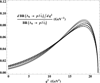
In Fig. 12 (left) one of the vector form factors is plotted, where the analytical parametrization [36] fitted to the LCSR prediction at low $q^{2}$ is used to extrapolate this form factor to the whole region of momentun transfer. One observes a reasonable agreement between the sum rules with different $\eta_{\Lambda_{b}}$-currents. The $\Lambda_{b}\to p\ell\nu_{\ell}$ decay width measurements combined with the calculated form factors provide an alternative source of $|V_{ub}|$ determination.

3 ​​​​​​. Lecture: Hadronic effects in $B\to K^{(*)}\ell^{+}\ell^{-}$

In this lecture I will discuss a more complex problem of calculating the hadronic input for exclusive flavour-changing neutral current (FCNC) decays. As we shall see, the LCSRs provide not only the form factors but also nonlocal hadronic matrix elements specific for these decays.

3.1 FCNC transitions and nonlocal hadronix matrix elements

(a)                                        (b)

Figure 13: Hadronic matrix elements of FCNC operators $O_{9,10}$ (a) and $O_{7}$ (b) in the $B\to K\ell^{+}\ell^{-}$ decays.

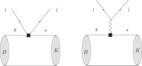
The $b\to s\,\ell^{+}\ell^{-}$ FCNC transitions, observed in the form of exclusive decays $B\to K^{(*)}\ell^{+}\ell^{-}$, are intensively studied at LHC and $B$ factories. The main interest in these decays is their sensitivity to the contributions of new heavy particles. In SM the $b\to s\ell^{+}\ell^{-}$ transitions are described by an effective Hamiltonian

$$H_{eff}=-\frac{4G_{F}}{\sqrt{2}}V_{tb}V_{ts}^{*}{\sum\limits_{i=1}^{10}}C_{i}(\mu)O_{i}\Big{|}_{\mu\sim m_{b}}\,,$$ (48)

where the loop diagrams with heavy SM particle ($t,Z,W$) are absorbed in the Wilson coefficients $C_{i}$. The lighter fields, including the $b$ quark field, form effective local operators $O_{i}$. The $B\to K^{(*)}\,\ell^{+}\ell^{-}$ decay amplitude

$$A(B\to K^{(*)}\ell^{+}\ell^{-})=\frac{G_{F}}{\sqrt{2}}V_{tb}V_{ts}^{*}\sum\limits_{i=1}^{10}C_{i}(\mu)\,\langle K^{(*)}\ell^{+}\ell^{-}\mid O_{i}\mid B\rangle\Big{|}_{\mu\sim m_{b}}$$ (49)

is written formally as a sum of matrix elements of effective operators between the initial and final states, weighted by their Wilson coefficients. The dependence on the scale $\mu$ indicates the separation of gluon radiative corrections with momenta larger and smaller than $\mu$ between the Wilson coefficients and hadronic matrix elements, respectively.

In the above, the dominant contributions to the amplitude (49) are given by the operators

$$O_{9(10)}=\frac{\alpha_{em}}{4\pi}[\bar{s}_{L}\gamma_{\mu}b_{L}]\ell\gamma^{\mu}(\gamma_{5})\ell,~{}~{}O_{7\gamma}=-\frac{em_{b}}{16\pi^{2}}[\bar{s}\sigma_{\mu\nu}(1+\gamma_{5})b]F^{\mu\nu}$$ (50)

with large coefficients $C_{9}(m_{b})\simeq 4.2$, $C_{10}(m_{b})\simeq-4.4$ and $C_{7}(m_{b})\simeq-0.3$. The corresponding diagrams are shown in Fig. 13. The new physics effects can substantially modify the coefficients $C_{9,10,7,...}$, and/or add new operators with different spin-parity combinations. In the contributions of $O_{9,10,7}$, the leptons are factorized out from the matrix elements in (49) and the only hadronic input one needs are the $B\to K^{(*)}$ form factors. The latter can be calculated with LCSR methods considered in the previous lecture.

However, at this stage the problem of determining the hadronic input in $B\to K^{(*)}\,\ell^{+}\ell^{-}$ is not yet solved. Note that the effective Hamiltonian (48) also contains effective operators without leptons or photon: the gluon-penguin $O_{8g}=-\frac{m_{b}}{8\pi^{2}}\bar{s}\sigma_{\mu\nu}(1+\gamma_{5})bG^{\mu\nu}$, 4-quark penguin operators $O_{3-6}$ with small Wilson coefficients and, most importantly, the current-current operators $O^{(c)}_{1}=[\bar{s}_{L}\gamma_{\rho}c_{L}][\bar{c}_{L}\gamma^{\rho}b_{L}]$ and $O^{(c)}_{2}=[\bar{c}_{L}\gamma_{\rho}c_{L}][\bar{s}_{L}\gamma^{\rho}b_{L}]$ of the “ordinary” weak interaction, with large coefficients $C_{1}(m_{b})\simeq 1.1$ and $C_{2}(m_{b})\simeq-0.25$, respectively . These operators also contribute to the $b\to s\ell^{+}\ell^{-}$ transition. In a combination with weak interaction, the lepton pair in the final state is electromagnetically emitted from one of the quark lines. The main problem is that the average distances between the photon emission and the weak interaction points are not necessarily short, hence these additional contributions to the decay amplitude are essentially nonlocal, and cannot be simply reduced to the form factors.

The following decomposition of the decay amplitude in terms of hadronic matrix elements:

$$A(B\to K^{(*)}\ell^{+}\ell^{-})=\frac{G_{F}}{\sqrt{2}}V_{tb}V_{ts}^{*}\frac{\alpha_{em}}{2\pi}\Bigg{[}(\bar{\ell}\gamma^{\rho}\gamma_{5}\ell\big{)}C_{10}\,\langle K^{(*)}|\bar{s}\gamma_{\rho}(1-\gamma_{5})b|B\rangle$$

$$+(\bar{\ell}\gamma^{\rho}\ell\big{)}\Big{(}C_{9}\,\langle K^{(*)}|\bar{s}\gamma_{\rho}b|B\rangle+C_{7}\,\frac{2(m_{b}+m_{s})}{q^{2}}q^{\nu}\langle K^{(*)}|\bar{s}i\sigma_{\nu\rho}(1+\gamma_{5})b|B\rangle$$

$$-\frac{32\pi^{2}}{q^{2}}\sum\limits_{i=1,2,...,6,8}C_{i}~{}{\cal H}^{\rho}_{i}\Big{)}\Big{]}$$ (51)

includes “direct” FCNC contributions proportional to $C_{9,10,7}$ multiplied by the $B\to K^{(*)}$ form factors and the nonlocal hadronic matrix elements

$${\cal H}_{i}^{\rho}(q,p)=\langle K^{(*)}(p)|i\!\int d^{4}x\,e^{iqx}\,T\{j^{\rho}_{em}(x),O_{i}(0)\}|B(p+q)\rangle$$ (52)

where $j_{em}^{\rho}=\sum\limits_{q=u,d,s,c,b}Q_{q}\bar{q}\gamma^{\rho}q$ is the quark electromagnetic current. The factor $1/q^{2}$ multiplying the nonlocal part of the amplitude is due to the photon propagator connecting the quarks with the lepton e.m. current.

Hereafter, for simplicity we consider the decay $B\to K\ell^{+}\ell^{-}$ with the kaon final state. The QCD LCSRs similar to the ones used to calculate $B\to\pi$ form factors (see the previous lecture), provide also $B\to K$ form factors. One has to replace the pion DA’s by kaon DA’s in the correlation function. Apart from the vector form factor $f_{BK}^{+}$, the tensor form factor $f_{BK}^{T}$ enters due to the $O_{7}$ operator. The LCSR results for all $B\to K$ form factors at $q^{2}\leq 12-15$ GeV² were updated in [49] and the numerical results can be found there. One obtains values up to 30% larger than for the corresponding $B\to\pi$ form factors, revealing a noticeable violation of $SU(3)_{flavour}$ symmetry. Our analysis of the $B\to K\ell^{+}\ell^{-}$ amplitude will be constrained by the large hadronic recoil region ($q^{2}<6-8$ GeV²) which is fully covered by LCSR form factors. Note that the alternative LCSR’s with $B$ DA’s also provide the $B\to K$ form factors [38], albeit with larger uncertainties.

The $B\to K\ell^{+}\ell^{-}$ amplitude, after inserting the form factors, reads:

$$A(B\to K\ell^{+}\ell^{-})={G_{F}\over\sqrt{2}}{\alpha_{em}\over\pi}V_{tb}V_{ts}^{\ast}\Bigg{[}\bar{\ell}\gamma_{\mu}\ell\,p^{\mu}\bigg{(}C_{9}f^{+}_{BK}(q^{2})$$

$$+{2(m_{b}+m_{s})\over m_{B}+m_{K}}C_{7}^{eff}f^{T}_{BK}(q^{2})+16\pi^{2}\!\!\!\!\!\sum\limits_{i=1,2,...,6,8}\!\!\!C_{i}~{}{\cal H}^{(BK)}_{i}(q^{2})\bigg{)}+\bar{\ell}\gamma_{\mu}\gamma_{5}\ell\,p^{\mu}C_{10}f^{+}_{BK}(q^{2})\bigg{]}\,,$$ (53)

where ${\cal H}_{i}^{(BK)}(q^{2})$ are the invariant amplitudes in the Lorentz-decomposition of (52).

3.2 Anatomy of the nonlocal hadronic matrix elements

The nonlocal contributions to the decay amplitude (53) can be cast in a form of corrections to the short-distance Wilson coefficient:

$$C_{9}\to C_{9}+\Delta C_{9}^{(BK)}(q^{2}),~{}~{}\mbox{where}~{}~{}\Delta C_{9}^{(BK)}(q^{2})=16\pi^{2}\!\!\!\sum\limits_{i=1,2,...,6,8}\!\!\!C_{i}~{}\frac{{\cal H}^{(BK)}_{i}(q^{2})}{f^{+}_{BK}(q^{2})}\,.$$ (54)

These corrections are $q^{2}$- and process-dependent and have to be estimated one by one for separate operators. The main question we address here is: are the nonlocal matrix elements ${\cal H}^{(BK)}_{i}(q^{2})$ calculable in QCD?

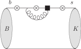
First of all one has to sort out various contributions diagrammatically. The most important diagram in LO (without additional gluons) is in Fig. 14: a virtual photon emission via intermediate quark loop originating from the current-current operators $O_{1,2}$ or from quark-penguin operators $O_{3-6}$. In Fig. 15 the same mechanism is accompanied by gluon exchanges including also the gluon penguin contribution. Not shown is the mechanism of the weak annihilation with virtual photon emission which has a small impact.

Calculation of these effects in $B\to K^{(*)}\ell^{+}\ell^{-}$ was done in the framework of HQET and QCD factorization approach [51] valid at $E_{K^{(*)}}\sim m_{b}/2$ and $m_{b}\to\infty$.

     

Figure 14: The quark-loop diagram of the nonlocal contribution to $B\to K\ell^{+}\ell^{-}$. The cross denotes the virtual photon emission point.

The results are obtained in the region of large hadronic recoil (small and intermediate $q^{2}$). The nonlocal amplitudes are expressed in terms of $B\to K$ form factors or factorized as a convolution of $B$- and light-meson DA’s with hard-scattering kernels. There are however two problems to clarify. First, at timelike $q^{2}\sim$ a few GeV², the virtual photon is emitted via intermediate on-shell vector mesons with the masses $m_{V}=\sqrt{q^{2}}$ ($V=\rho,\omega,\phi,J/\psi,...)$ rather than off quarks, hence the accuracy of the perturbative treatment has to be assessed.

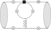
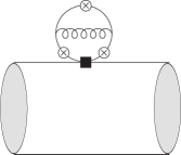
The second related problem is the role of soft virtual gluons in the nonlocal amplitudes. The diagrams shown schematically in Fig. 16 are “fully nonfactorizable”, i.e., with no possibility to separate a hard scattering amplitude from the long-distance one. The whole hadronic matix element has to be considered as a nonperturbative object.

(a)                                        (b)
  

(c)                                       (d)

Figure 15: Factorizable diagrams with hard gluon exchanges

(a)                               (b)

Figure 16: Soft-gluon nonfactorizable diagrams

3.3 Charm-loop effect and light-cone OPE

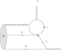
Let me briefly outline the approach to nonlocal hadronic matrix elements applied in [49] where the two problems formulated above were addressed, concentrating on the most important (due to large Wilson coefficients) part of the nonlocal amplitude generated by the operators $O_{1,2}$.

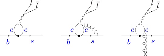
(a)                            (b)                            (c)

Figure 17: $\bar{c}c$-quark loop effect at quark level

This is a combination of the $(\bar{s}c)(\bar{c}b)$ weak interaction and the $(\bar{c}c)(\bar{\ell}\ell)$ e.m.interaction, which effectively leads to $b\to s\ell^{+}\ell^{-}$ transition due to the fact that the charmed quark pair appears in the intermediate state only.

The leading order diagram shown in Fig. 17(a) contains the simple $c$-quark loop similar to the heavy-light loop in the two-point correlation function considered in the first lecture. Also here the physics depends on the region of the $q^{2}$ variable. At $q^{2}\to m^{2}_{J/\psi},...$ the charm loop turns into an on-shell hadronic $J/\psi$ state, and the semileptonic decay we are considering becomes a combination of nonleptonic weak transition $B\to J/\psi K$, followed by the e.m. decay $J/\psi\to\ell^{+}\ell^{-}$. At larger $q^{2}$, the $\psi(2S)$ and other charmonia with $J^{P}=1^{-}$, as well as the open-charmed pairs contribute, with increasing masses up to the kinematical threshold $\sqrt{q^{2}}=m_{B}-m_{K}$. To avoid a “direct” charmonium background, the $q^{2}$ intervals around $J/\psi$ and $\psi(2S)$ are subtracted from the measured lepton-pair mass distributions in $B\to K^{(*)}\ell^{+}\ell^{-}$. This subtraction does not however exclude the contribution of intermediate virtual ${\bar{c}}c$ state below the charmonium levels. Can one use the “loop plus corrections” ansatz for this contribution and at which $q^{2}$?

To investigate this question, let us isolate the charm-loop effect in the decay amplitude:

$$A(B\to K^{(*)}\ell^{+}\ell^{-})^{(O_{1,2})}=-(4\pi\alpha_{em}Q_{c})\frac{4G_{F}}{\sqrt{2}}V_{tb}V^{*}_{ts}\frac{\bar{\ell}\gamma^{\mu}\ell}{q^{2}}{\cal H}_{\mu}^{(B\to K^{(*)})}\,,$$ (55)

where the hadronic matrix element:

$${\cal H}^{(B\to K)}_{\mu}(p,q)=i\int d^{4}xe^{iq\cdot x}\langle K(p)|T\Big{\{}\bar{c}(x)\gamma_{\mu}c(x)\,,\Big{[}C_{1}O_{1}(0)+C_{2}O_{2}(0)\Big{]}\Big{\}}|B(p+q)\rangle\,,$$ (56)

contains the $T$-product of two $\bar{c}c$ operators

$${\cal C}^{a}_{\mu}(q)=\int d^{4}xe^{iq\cdot x}T\Big{\{}\bar{c}(x)\gamma_{\mu}c(x),\bar{c}_{L}(0)\Gamma^{a}c_{L}(0)\Big{\}}\,.$$ (57)

As shown in [49], only at momentum transfers, much lower than the charm-anticharm threshold, $q^{2}\ll 4m_{c}^{2}$ one is allowed to use the operator-product expansion (OPE), and, importantly the expansion is near the light-cone. The dominant region in this $T$-product is $\langle x^{2}\rangle\sim 1/(2m_{c}-\sqrt{q^{2}})^{2}$. In this region the $T$- product of $\bar{c}c$-operators can be expanded near $x^{2}\sim 0$, schematically,

$$T\{\bar{c}(x)\gamma_{\mu}c(x),\bar{c}_{L}(0)\gamma_{\rho}c_{L}(0)\}=C_{0}^{\mu\rho}(x^{2},m_{c}^{2})+\mbox{two-gluon term}+...$$ (58)

$$T\{\bar{c}(x)\gamma_{\mu}c(x),\bar{c}_{L}(0)\gamma_{\rho}\frac{\lambda^{a}}{2}c_{L}(0)\}=\int\limits_{0}^{1}duC_{1}^{\mu\rho\alpha\beta}(x^{2},m_{c}^{2},u)G^{a}_{\alpha\beta}(ux)+...$$ (59)

The leading-order term of this expansion $C_{0}^{\mu\rho}(x^{2},m_{c}^{2})$ is reduced to the simple $\bar{c}c$ loop. Substituting this term back in the decay amplitude (56), after the $x$-integration one obtains

$${\cal O}_{\mu}(q)=(q_{\mu}q_{\rho}-q^{2}g_{\mu\rho})\frac{9}{32\pi^{2}}~{}g(m_{c}^{2},q^{2})\bar{s}_{L}\gamma^{\rho}b_{L}\,,$$ (60)

the simple loop function denoted as $g(m_{c}^{2},q^{2})$ times the $b\to s$ transition current (see Fig. 17a). After taking the hadronic matrix element we recover the factorizable part of the amplitude:

$$\Big{[}{\cal H}^{(B\to K)}_{\mu}(p,q)\Big{]}_{fact}=\left(\frac{C_{1}}{3}+C_{2}\right)\langle K(p)|{\cal O}_{\mu}(q)|B(p+q)\rangle\,,$$ (61)

factorized in the loop function and $B\to K$ form factor (Fig. 14). Note that at this level of OPE there is no difference between light-cone ($x^{2}\sim 0$) and local ($x\sim 0$) expansion. There are also perturbative gluon corrections to this operator, one of them shown in Fig. 17(b). They are factorizable too after taking the hadronic matrix elements. For them one can use the results of [51], with the only difference that now we consistently avoid the region $q^{2}\sim 4m_{c}^{2}$.

Figure 18: Correlation function used to calculate the nonfactorizable hadronic matrix element (63).

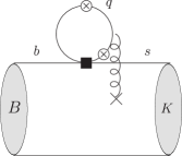
The genuine nonfactorizable effect is related to the one-gluon term (59) in the light-cone OPE. It is obtained using the $c$-quark propagator in the external gluon field and yields a new nonlocal operator depicted in Fig. 17(c):

$$\widetilde{{\cal O}}_{\mu}(q)=\int d\omega\,I_{\mu\rho\alpha\beta}(q,m_{c},\omega)\bar{s}_{L}\gamma^{\rho}\delta[\omega-{(in_{+}{\cal D})\over 2}]\widetilde{G}_{\alpha\beta}b_{L}\,\,,$$ (62)

where the coefficient $I_{\mu\rho\alpha\beta}(q,m_{c},\omega)$ represents a loop function with gluon insertion and $n_{+}$ is the light-like vector defined in $B$ rest frame, so that $q\sim(m_{b}/2)n_{+}$. More details can be found in [49]. The gluon emission term yields a new nonfactorizable hadronic matrix element:

$$\Big{[}{\cal H}^{(B\to K)}_{\mu}(p,q)\Big{]}_{nonfact}=2C_{1}\langle K(p)|\widetilde{{\cal O}}_{\mu}(q)|B(p+q)\rangle\,.$$ (63)

which is not reduced to simple $B\to K$ form factors and corresponds to the diagram in Fig. 16a.

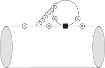
To calculate the soft-gluon hadronic matrix element (63), the method of LCSRs with $B$ meson DA’s outlined in the previous lecture was used in [49], introducing a correlation function:

$${\cal F}^{(B\to K)}_{\nu\mu}(p,q)=i\int d^{4}ye^{ip\cdot y}\langle 0|T\{j_{\nu}^{K}(y)\widetilde{{\cal O}}_{\mu}(q)\}|B(p+q)\rangle\,.$$ (64)

The diagram of the correlation function is shown in Fig. 18 and the OPE contains the 3-particle DAs of $B$ meson.

Summarizing, the charm-loop effect in $B\to K\ell^{+}\ell^{-}$ is a sum of two hadronic matrix elements calculated in QCD, but this calculation is only valid at $q^{2}\ll 4m_{c}^{2}$. In [49] the perturbative corrections were not yet included. Still, to have some idea on the importance of the charm loop effect let me quote the value $\Delta C^{(\bar{c}c)}_{9}(0)=0.17^{+0.09}_{-0.18}$ obtained for the charm-loop correction to the effective coefficient $C_{9}$.

3.4 Hadronic input for $B\to K\ell^{+}\ell^{-}$ decay

(a)                                                       (b)

Figure 19: [50] The contribution of nonlocal hadronic effects in a form of correction $\Delta C_{9}(q^{2})$ to the Wilson coefficient $C_{9}$ in the physical region of $B\to K\ell^{+}\ell^{-}$ decay obtained from the hadronic dispersion relation, fitted to the QCD calculation at $q^{2}<0$. The shaded areas indicate the uncertainty of the predictions. The dashed lines are the predictions of QCD factorization [51].

Following the method suggested in [49], in [50] a complete “bookkeeping” of nonlocal contributions to $B\to K\ell^{+}\ell^{-}$ decay amplitude was done. The soft-gluon effects originating from quark loops with various flavours were calculated from LCSRs, including also the soft-gluon contribution due to the gluon-penguin operator shown in Fig. 16b. In addition also the perturbative gluon exchanges (Fig. 15) were taken into account employing the results of [51]. Note that the latter contributions generate an imaginary part in $\Delta C_{9}^{(BK)}(q^{2})$ as explained in details in [50]. Furthermore, after including the photon emission from the light quarks, the $q^{2}$ region accessible to OPE was shifted towards large negative values of $q^{2}$, to stay sufficiently far from all hadronic thresholds.

This calculation was then used for a phenomenological analysis of the $B\to K\ell^{+}\ell^{-}$ decay. To access the timelike $q^{2}$ region where OPE is not applicable, the hadronic dispersion relation in the variable $q^{2}$ was employed [49, 50] for the nonlocal hadronic amplitude. To illustrate the idea, let us return to the previous subsection where only the charm-loop effect was taken into account. In this case the dispersion relation contains only hadronic states with $\bar{c}c$ flavour content: [49]:

$${\cal H}^{(B\to K)}(q^{2})={\cal H}^{(B\to K)}(0)+q^{2}\Big{[}\sum_{\psi=J/\psi,\psi(2S)}\frac{f_{\psi}A_{B\psi K}}{m_{\psi}^{2}(m_{\psi}^{2}-q^{2}-im_{\psi}\Gamma^{tot}_{\psi})}$$

$$+\int_{4m_{D}^{2}}^{\infty}ds\frac{\rho(s)}{s(s-q^{2}-i\epsilon)}\Big{]}.$$ (65)

The QCD calculation at small $q^{2}$ is used to fit the parameters of this relation and then it is used in the timelike region. In addition, the absolute values of the residues $|f_{\psi}A_{B\psi K}|$ are fixed from experimental data on nonleptonic decays $B\to J/\psi K$, $B\to\psi(2S)K$ and leptonic decays of charmonium [16].

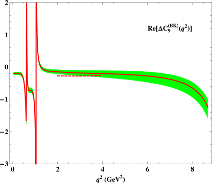
For a full phenomenological analysis of nonlocal amplitude ${\cal H}^{(B\to K)}(q^{2})$ in the semileptonic region below charmonium resonances a more complete dispersion relation was used in[50], adding vector mesons with light flavours to the r.h.s. of Eq. (65). The main outcome of this analysis is displayed in Fig. 19 where the resulting correction to $C_{9}$ due to all nonlocal effects is plotted, obtained from the dispersion relation fitted to the OPE results at negative $q^{2}$ . Adding these correction to the short-distance coefficients and employing the $B\to K$ form factors from LCSRs the partial width of $B\to K\ell^{+}\ell^{-}$ was predicted in [50]. It is displayed in Fig. 20. The influence of nonlocal effects on the decay observables is very moderate and the form factor uncertainty still dominates. For $B\to K^{*}\ell^{+}\ell^{-}$ decay the full analysis still has to be done. Hints that the nonlocal hadronic effects in this process are more pronounced than in the kaon mode come from the results for the charm-loop contribution obtained in [49].

Let me emphasize that in future studies of FCNC semileptonic decays of $B$ mesons based on more accurate data the effects studied in this lecture are indispensable. Without them the predictions for SM observables are incomplete. The methods based on OPE, LCSRs and dispersion relations combined with QCD factorization for perturbative contributions provide a useful tool to tackle this problem.

Figure 20: [50] Differential partial branching fraction of $B\to K\ell^{+}\ell^{-}$. The darker (brighter) shaded area indicates the uncertainties including(excluding) the one from the $B\to K$ form factors. The long-dashed line corresponds to the width calculated without nonlocal hadronic effects.

References

- [1] M. A. Shifman, A. I. Vainshtein and V. I. Zakharov, Nucl. Phys. B 147 (1979) 385, 448.
- [2] M. A. Shifman, Prog. Theor. Phys. Suppl. 131, 1 (1998) [hep-ph/9802214].
-
[3]
V. A. Novikov, L. B. Okun, M. A. Shifman, A. I. Vainshtein, M. B. Voloshin and V. I. Zakharov,
Phys. Rept. 41, 1 (1978);
L. J. Reinders, H. Rubinstein and S. Yazaki, Phys. Rept. 127, 1 (1985);
S. Narison, World Sci. Lect. Notes Phys. 26, 1 (1989). - [4] A. Khodjamirian and R. Rückl, Adv. Ser. Direct. High Energy Phys. 15, 345 (1998) [hep-ph/9801443].
- [5] P. Colangelo and A. Khodjamirian, In Shifman, M. (ed.): At the frontier of particle physics, vol. 3 1495-1576 [hep-ph/0010175].
- [6] V. M. Braun, In Rostock 1997, Progress in heavy quark physics, 105-118 [hep-ph/9801222].
- [7] I. Adachi et al. [Belle Collaboration], Phys. Rev. Lett. 110, 131801 (2013).
- [8] R.Aaij et al. [LHCb Collaboration], Phys. Rev. Lett. 110 (2013) 021801. CMS and LHCb Collaborations [CMS and LHCb Collaboration], CMS-PAS-BPH-13-007.
- [9] B. L. Ioffe, Phys. Atom. Nucl. 66, 30 (2003) [Yad. Fiz. 66, 32 (2003)] [hep-ph/0207191].
- [10] T. M. Aliev and V. L. Eletsky, Sov. J. Nucl. Phys. 38 (1983) 936 [Yad. Fiz. 38 (1983) 1537].
- [11] K. G. Chetyrkin and M. Steinhauser, Eur. Phys. J. C 21, 319 (2001).
- [12] V. A. Novikov, M. A. Shifman, A. I. Vainshtein and V. I. Zakharov, Fortsch. Phys. 32, 585 (1984).
- [13] P. Gelhausen, A. Khodjamirian, A. A. Pivovarov and D. Rosenthal, Phys. Rev. D 88, 014015 (2013).
- [14] M. Jamin and B. O. Lange, Phys. Rev. D 65, 056005 (2002).
- [15] K. Chetyrkin, J. H. Kuhn, A. Maier, P. Maierhofer, P. Marquard, M. Steinhauser and C. Sturm, Theor. Math. Phys. 170, 217 (2012) [arXiv:1010.6157 [hep-ph]].
- [16] J. Beringer et al. [Particle Data Group Collaboration], Phys. Rev. D 86, 010001 (2012), see also www.pdg.gov.
- [17] B. Dehnadi, A. H. Hoang, V. Mateu and S. M. Zebarjad, JHEP 1309, 103 (2013).
[18]
K. G. Chetyrkin and A. Khodjamirian,
Eur. Phys. J. C 46 (2006) 721;
M. Jamin, J. A. Oller and A. Pich, Phys. Rev. D 74 (2006) 074009. - [19] H. Leutwyler, Phys. Lett. B 378, 313 (1996).
- [20] A. Bazavov et al. [Fermilab Lattice and MILC Collaborations], Phys. Rev. D 85, 114506 (2012).
- [21] R. J. Dowdall, C. T. H. Davies, R. R. Horgan, C. J. Monahan and J. Shigemitsu, arXiv:1302.2644 [hep-lat].
- [22] C. T. H. Davies, C. McNeile, E. Follana, G. P. Lepage, H. Na and J. Shigemitsu, Phys. Rev. D 82 (2010) 114504.
- [23] I. I. Balitsky, V. M. Braun and A. V. Kolesnichenko, Sov. J. Nucl. Phys. 44 1028 (1986) [Yad. Fiz. 44 1582 (1986)]; Nucl. Phys. B 312, 509 (1989).
- [24] V. L. Chernyak and I. R. Zhitnitsky, Nucl. Phys. B 345, 137 (1990).
- [25] V. M. Belyaev, A. Khodjamirian and R. Rückl, Z. Phys. C 60, 349 (1993); V. M. Belyaev, V. M. Braun, A. Khodjamirian and R. Rückl, Phys. Rev. D 51, 6177 (1995).
- [26] A. Khodjamirian, R. Ruckl, S. Weinzierl and O. I. Yakovlev, Phys. Lett. B 410, 275 (1997);
- [27] E. Bagan, P. Ball and V. M. Braun, Phys. Lett. B 417, 154 (1998).
- [28] P. Ball and R. Zwicky, Phys. Rev. D 71, 014015 (2005).
- [29] G. Duplancic, A. Khodjamirian, T. Mannel, B. Melic and N. Offen, JHEP 0804, 014 (2008).
- [30] A. Bharucha, JHEP 1205, 092 (2012).
[31]
V. L. Chernyak and A. R. Zhitnitsky,
JETP Lett. 25, 510 (1977);
A. V. Efremov and A. V. Radyushkin, Phys. Lett. B 94, 245 (1980). - [32] G. P. Lepage and S. J. Brodsky, Phys. Lett. B 87, 359 (1979).
- [33] P. Ball, V. M. Braun and A. Lenz, JHEP 0605, 004 (2006).
- [34] A. Khodjamirian, T. Mannel, N. Offen and Y. -M. Wang, Phys. Rev. D 83 (2011) 094031.
[35]
E. Dalgic, A. Gray, M. Wingate, C. T. H. Davies, G. P. Lepage and J. Shigemitsu,
Phys. Rev. D 73, 074502 (2006)
[Erratum-ibid. D 75, 119906 (2007)];
J. A. Bailey, C. Bernard, C. E. DeTar, M. Di Pierro, A. X. El-Khadra, R. T. Evans, E. D. Freeland and E. Gamiz et al., Phys. Rev. D 79 (2009) 054507 [arXiv:0811.3640 [hep-lat]]. - [36] C. Bourrely, I. Caprini and L. Lellouch, Phys. Rev. D 79, 013008 (2009) [Erratum-ibid. D 82, 099902 (2010)] .
- [37] A. Khodjamirian, C. Klein, T. Mannel and N. Offen, Phys. Rev. D 80 (2009) 114005.
- [38] A. Khodjamirian, T. Mannel and N. Offen, Phys. Lett. B 620, 52 (2005); Phys. Rev. D 75, 054013 (2007).
- [39] F. De Fazio, T. Feldmann and T. Hurth, Nucl. Phys. B 733, 1 (2006) [Erratum-ibid. B 800, 405 (2008)] .
- [40] M. Beneke and T. Feldmann, Nucl. Phys. B 592, 3 (2001).
- [41] A. G. Grozin and M. Neubert, Phys. Rev. D 55, 272 (1997).
- [42] A. G. Grozin, Int. J. Mod. Phys. A 20, 7451 (2005) [hep-ph/0506226].
- [43] V. M. Braun, D. Y. .Ivanov and G. P. Korchemsky, Phys. Rev. D 69, 034014 (2004) .
- [44] M. Beneke and J. Rohrwild, Eur. Phys. J. C 71, 1818 (2011) .
- [45] V. M. Braun and A. Khodjamirian, Phys. Lett. B 718, 1014 (2013) .
- [46] S. Faller, A. Khodjamirian, C. .Klein and T. .Mannel, Eur. Phys. J. C 60, 603 (2009) .
- [47] A. Khodjamirian, C. Klein, T. Mannel and Y. -M. Wang, JHEP 1109, 106 (2011).
- [48] V. Braun, R. J. Fries, N. Mahnke and E. Stein, Nucl. Phys. B 589 (2000) 381 [Erratum-ibid. B 607 (2001) 433]; V. M. Braun, A. Lenz, N. Mahnke and E. Stein, Phys. Rev. D 65, 074011 (2002); A. Lenz, M. Gockeler, T. Kaltenbrunner and N. Warkentin, Phys. Rev. D 79, 093007 (2009).
- [49] A. Khodjamirian, T. Mannel, A. A. Pivovarov and Y. -M. Wang, JHEP 1009, 089 (2010).
- [50] A. Khodjamirian, T. Mannel and Y. M. Wang, JHEP 1302, 010 (2013).
- [51] M. Beneke, T. Feldmann and D. Seidel, Nucl. Phys. B 612, 25 (2001).