Exact Simulation of Non-stationary
Reflected Brownian Motion

Abstract

This paper develops the first method for the exact simulation of reflected Brownian motion (RBM) with non-stationary drift and infinitesimal variance. The running time of generating exact samples of non-stationary RBM at any time $t$ is uniformly bounded by $\mathcal{O}(1/\bar{\gamma}^{2})$ where $\bar{\gamma}$ is the average drift of the process. The method can be used as a guide for planning simulations of complex queueing systems with non-stationary arrival rates and/or service time.

1 Introduction

This paper is concerned with the exact simulation of reflected Brownian motion (RBM) with non-stationary drift and infinitesimal variance. Our interest in this model stems from the fact that RBM is commonly used as a stylized representation of a single-station queue (and often as a model for extracting numerical approximations to queues in heavy traffic); see Iglehart and Whitt (1970).

In many (indeed most) real-world applications of queueing models, there exist non-stationarities in the arrival rates and/or service time requirements that are induced by time-of-day, day-of-week, or seasonality effects. In addition, in some situations (as in production or inventory contexts), there may also be non-stationarities associated with rising or falling demand for a product, as it is introduced to the marketplace or becomes obsolete. In such applications, a simplified description of the workload process $X=(X(t):t\geq 0)$ is to postulate that it satisfies the stochastic differential equation (SDE)

$$dX(t)=\mu(t)dt+\sigma(t)dB(t)+dL(t),$$ (1.1)

where $L=(L(t):t\geq 0)$ is the continuous non-decreasing process satisfying

$$I(X(t)>0)dL(t)=0$$

for $t\geq 0$, $B=(B(t)\colon t\geq 0)$ is standard Brownian motion, and $\mu=(\mu(t)\colon t\geq 0)$ and $\sigma=(\sigma(t)\colon t\geq 0)$ are given (measurable) deterministic functions. Note that this stylized model permits both the instantaneous drift and volatility to be separately specified, unlike the non-stationary $M(t)/M(t)/1$ model that has been previously studied in the queueing literature (see, for example, Massey (1981)) in which the instantaneous drift must always match the instantaneous volatility. Assuming $X(0)=x$, our goal here is to provide an algorithm for generating $X(t)$ with a complexity that is bounded in $t$, at least when $X$ empties infinitely often almost surely (a.s.). If the coefficient functions are stationary (so that $\mu(\cdot)$ and $\sigma(\cdot)$ are constant) and we send $t\rightarrow\infty$, it is evident that this is a non-stationary analog to the exact simulation problem for positive recurrent Markov processes. Hence, we use the terminology “exact simulation” to also refer to our non-stationary problem.

Of course, if RBM has stationary drift and infinitesimal variance, the transient and steady-state distributions of $X$ are then known in closed form, and simulation is unnecessary. In the non-stationary context, the transition density $p(t,x,y)dy\ (\stackrel{{\scriptstyle\Delta}}{{=}}P(X(t)\in dy|X(0)=x))$ would be expected to satisfy the Kolmogorov forward partial differential equation (PDE)

$$\frac{\partial}{\partial s}p(s,x,y)=\frac{1}{2}\sigma^{2}(s)\frac{\partial^{2}}{\partial y^{2}}p(s,x,y)-\mu(s)\frac{\partial}{\partial y}p(s,x,y),\mbox{\ \ \ \ \ \ $0<s\leq t,$}$$ (1.2)

subject to $P(X(0)\in dy|X(0)=x)=\delta_{x}(dy)$ and

$$\frac{\sigma(s)^{2}}{2}\frac{\partial}{\partial y}p(s,x,0)-\mu(s)p(s,x,0)=0,\mbox{\ \ \ \ \ \ $0<s\leq t.$}$$

Unlike the stationary case, this PDE has no known closed-form solution, and would need to be solved numerically. This paper provides an efficient computational alternative to numerically solving the above PDE, which is especially attractive when the time horizon $t$ of interest is large.

As indicated above, $X$ can be used as a basis model for studying a queue with non-stationary dynamics. But in many applications, we would prefer to use a “finer grain” and more realistic simulation model, rather than RMB itself, as a mathematical description of the real-world system under consideration. One intuitively expects that such models “lose memory”, in the sense that the distribution at time $t$ often will be insensitive to the state at time $t-u$, provided that $u$ is chosen large enough. In the presence of such insensitivity, one can (for example) initialize the system in the empty state at time $t-u$ and execute the fine-grain simulation only over $[t-u,t]$ rather than $[0,t]$, thereby generating significant computational savings. Thus, identifying an appropriate value of $u$ is of significant interest.

While estimating the “loss of memory” for the underlying detailed model would be extremely challenging, we will argue in Section 2, via a coupling argument, that it can be readily estimated for the simplified RBM model. Simulation of the non-stationary RBM can then be used to determine how large $u$ should be chosen for the detailed model (perhaps by multiplying the RBM’s value of $u$ by a factor of 2, in order to account for the model approximation error). Thus, non-stationary RBM can be viewed as a simulation planning tool for more complex detailed queueing simulations, in the same sense that Whitt (1989) and Asmussen (1992) argue that RBM with stationary dynamics is an appropriate tool for planning steady-state queueing simulations.

We note, in passing, that a special case of our problem arises when $\mu(\cdot)$ and $\sigma(\cdot)$ are periodic (with the same period). Various theoretical results are known for such periodic models; see for example, Harrison and Lemoine (1977), Heyman and Whitt (1984), Asmussen and Thorisson (1987), and Bambos and Walrand (1989). In addition, when $\mu(\cdot)$ and $\sigma(\cdot)$ are stochastic (but independent of $B=(B(t):t\geq 0))$, the problem of simulating $X$ reduces to the deterministic case considered here upon conditioning on $\mu$ and $\sigma$. In this way, our method can cover (for example) RBM with non-Markov $\mu$ and $\sigma$.

The remainder of this paper is organized as follows: Section 2 discusses how to plan the simulation of a queueing model with non-stationary inputs. Sections 3 and 4 develop the main exact simulation methods of time-dependent RBM. Sections 5 and 6 explain the implementation details. Section 6 analyzes the algorithm. Section 7 provides numerical results.

2 Planning Simulations of Non-stationary
Queueing Models

Our goal here is to study the rate at which the non-stationary RBM $X$ “loses memory”. In view of our discussion in the introduction, we wish to specifically answer the following question:

How large must we choose $u$ so that the RBM started at time $t-u$ from the idle state (i.e. no workload in the system) will have a distribution at time $t$ that is close to that of the RBM at time $0$ from its initial workload $x$?

For $0\leq s\leq t$, let $(X_{s}(t):t\geq s)$ be the solution to (1.1) conditional on $X_{s}(s)=0$, and let $\|\cdot\|$ be the total variation norm. Also, set

$$\hat{v}_{t}=\sup{\{r\in[0,t]\colon X(r)=0}\}$$

with the convention that if $X$ does not visit $0$ over $[0,t]$, then $\tilde{v}_{t}=-\infty$.

Proposition 2.1.

For $0\leq s\leq t$,

$$\|\mathbb{P}(X_{s}(t)\in\cdot)-\mathbb{P}(X(t)\in\cdot\mid X(0)=x)\|\leq\mathbb{P}(\tilde{v}_{t}\leq s\mid X(0)=x).$$

Proposition 2.1 provides an answer to our question: For a given error tolerance $\epsilon$, we should choose $u$ so that

$$\mathbb{P}(\tilde{v}_{t}\leq t-u\mid X(0)=x)=\mathbb{P}(t-\tilde{v}_{t}\geq u\mid X(0)=x)\leq\epsilon.$$

Proof of Proposition 2.1. Let

$$\widetilde{Y}(t) =\int_{0}^{t}\!\mu(s)\,ds+\int_{0}^{t}\!\sigma(s)\,dB(s)$$

$$\widetilde{M}(s,t) =-\displaystyle\inf_{s\leq r\leq t}\widetilde{Y}(r)$$

for $0\leq s\leq t$. It is well known that the solution to the SDE (1.1), conditional on $X(0)=x$, can be explicitly compared in terms of $\widetilde{Y}$; specifically,

$$X(t)=x+\widetilde{Y}(t)+\displaystyle\sup_{0\leq s\leq t}{\max\left(-x-\widetilde{Y}(s),0\right)};$$ (2.1)

see, for example, p. 20 of Harrison (1985).

Relation (2.1) can be re-expressed as

$$X(t)=\begin{cases}\widetilde{Y}(t)+\widetilde{M}(0,t)&\mbox{if }\widetilde{M}(0,t)\geq x,\\ \widetilde{Y}(t)+x&\mbox{if }\tilde{M}(0,t)\leq x.\end{cases}$$ (2.2)

We can couple $X_{s}$ to $X$ by noting that $X_{s}(t)$ can similarly be expressed as

$$X_{s}(t)=\widetilde{Y}(t)+\widetilde{M}(s,t).$$

Hence, $X_{s}(t)=X(t)$ whenever $\widetilde{M}(s,t)=\widetilde{M}(0,t)\geq x$. But $\widetilde{M}(s,t)=\widetilde{M}(0,t)\geq x$ precisely whenever $X$ visits $0$ on $[s,t]$, which is equivalent to assertions that $\widetilde{v}_{t}\geq s$. Consequently, coupling between $X$ and $X_{s}$ establishes that

$$\mathbb{P}(X_{s}(t)\in\cdot\ ,\ \tilde{v}_{t}\geq s)=\mathbb{P}(X(t)\in\cdot\ ,\tilde{v}_{t}\geq s\mid X(0)=x),$$

proving that

$$\displaystyle\sup_{B}\Big{|}\mathbb{P}(X_{s}(t)\in B)-\mathbb{P}(X(t)\in B\mid X(0)=x)\Big{|}\leq\mathbb{P}(\tilde{v}_{t}<s\mid X(0)=x).$$

 

Thus, the key random variable (rv) to simulate for purposes of planning queueing simulations is $t-\tilde{v}_{t}$. On the other hand, when $X$ itself is the best model of interests, our focus is on $X(t)$. So, our goal in this paper is to efficiently simulate the pair $(t-\tilde{v}_{t},X(t))$. In particular, our interest is in an algorithm for generating $(t-\tilde{v}_{t},X(t))$ having a computational complexity independent of $t$.

To pursue this objective, it is convenient to use a distributionally equivalent representation for $(t-\tilde{v}_{t},X(t))$. To this end, let

$$Y^{\star}(r)=\widetilde{Y}(t)-\widetilde{Y}(t-r)$$

be the time-reversal of $\widetilde{Y}$ (time-reversed from time $t$). We now express $t-\tilde{v}_{t}$ and $X(t)$ in terms of the time-reversal $Y^{\star}$.

Note that

$$X(t)=\begin{cases}\displaystyle\sup_{0\leq s\leq t}Y^{\star}(s),&\mbox{if }\displaystyle\sup_{0\leq s\leq t}Y^{\star}(s)\geq x+Y^{\star}(t)\\ \\ x+Y^{\star}(t),&\mbox{if}\displaystyle\sup_{0\leq s\leq t}Y^{\star}(s)<x+Y^{\star}(t).\end{cases}$$ (2.3)

As for $\tilde{v}_{t}$, it is (in the event $\{\widetilde{M}(0,t)\geq x\}$) the largest value of $r\in[0,t]$ for which

$$\widetilde{Y}(r)=\inf_{0\leq s\leq r}\widetilde{Y}(s).$$

Since $\tilde{v}_{t}$ is the largest such value and $\widetilde{Y}$ is continuous,

$$\widetilde{Y}(v)>\inf_{0\leq s\leq t}\widetilde{Y}(s).$$

for $v\in[\tilde{v}_{t},t]$. Consequently,

$$\widetilde{Y}(\tilde{v}_{t})=\inf_{0\leq s\leq t}\widetilde{Y}(s).$$

Because $\widetilde{Y}(\cdot)$ has a unique minimizer on $[0,t]$, $\tilde{v}_{t}=\arg\min(\widetilde{Y}(s)\colon 0\leq s\leq t)$. It is then immediate that $v^{\star}_{t}=t-\tilde{v}_{t}$, where

$$v^{\star}_{t}=\arg\max\Big{(}Y^{\star}(s):0\leq s\leq t\Big{)}.$$

We conclude that

$$t-\tilde{v}_{t}=\begin{cases}v^{\star}_{t}&\mbox{if }\displaystyle\sup_{0\leq s\leq t}Y^{\star}(s)\geq x+Y^{\star}(t)\\ \infty&\mbox{else }.\end{cases}$$ (2.4)

Thus, the random vector $(t-\tilde{v}_{t},X(t))$ is determined by $\Big{(}v^{\star}_{t},\displaystyle\sup_{0\leq s\leq t}Y^{\star}(s),Y^{\star}(t)\Big{)}$.

Finally, note that $(Y^{\star}(s)\colon s\geq 0)$ has the same law as the process

$$Y(s)=\int_{0}^{s}\mu^{\prime}(r)dr+\int_{0}^{s}\sigma^{\prime}(r)dB(r),$$

where $\mu^{\prime}(r)\triangleq\mu(t-r)$ and $\sigma^{\prime}(r)=\sigma(t-r)$ for $r\geq 0$. Thus, the remainder of this section is concerned with generating the triplet $(v_{t},M(t),Y(t))$ ($\buildrel D\over{=}(v^{\star}_{t},\displaystyle\sup_{0\leq s\leq t}Y^{\star}(s),Y^{\star}(t))$), where

$$M(t)=\displaystyle\max_{0\leq s\leq t}Y(s)$$ (2.5)

$$v_{t}=\arg\max(Y(s):0\leq s\leq t),$$

and $\buildrel D\over{=}$ denotes equality in distribution.

Suppose now that the drift and volatility functions are periodic. Without loss of generality, we assume that the period is one. In this periodic setting, $\mu^{\prime}(\cdot)=\mu(n+b-\cdot)$ and $\sigma^{\prime}(\cdot)=\sigma(n+b-\cdot)$ are independent of $n\in\mathbb{Z}_{+}$ for $0\leq b\leq 1$, so that our above argument establishes that $(n+b-\tilde{v}_{n+b},X(n+b))$ can be determined from the joint distribution of $\left(v_{n+b},M(n+b),Y(n+b)\right)$. Furthermore, if

$$\int_{0}^{1}\mu(s)\operatorname{d}s<0,$$ (2.6)

then $Y(t)\rightarrow-\infty$ a.s. as $t\rightarrow\infty$, and there exist finite-valued rev’s $v^{b}_{\infty}$ and $M^{b}_{\infty}$ such that

$$(v_{t},M(t))\rightarrow(v^{b}_{\infty},M^{b}_{\infty})$$

as $t\rightarrow\infty$. In addition,

$$X(n+b)\Rightarrow M_{\infty}^{b}$$

as $n\rightarrow\infty$. Hence, if $(v_{t},M(t),Y(t))$ can be generated with a complexity independent of $t$, one arrive at an algorithm that can generate $(n+b-\tilde{v}_{n+b},X(n+b))$ with a complexity independent of $n$. Furthermore, if $M_{\infty}^{b}$ can be sampled, this converts to an exact sampling algorithm for the equilibrium of $(X(n+b):n\geq 0)$.

This leads naturally to the following re-formulation of the key issue to be addressed in this chapter:

Under appropriate hypotheses, provide an algorithm for generating $M(\infty)$ in finite expected time, and generating $(v_{t},M(t),Y(t))$ with a complexity independent of $t$.

For a non-periodic specification of $\mu^{\prime}(\cdot)$ and $\sigma^{\prime}(\cdot)$ for which $Y(t)\rightarrow-\infty$ as $t\rightarrow\infty$ a.s., we can view a solution to the above problem as providing an exact sampling algorithm for the rv $X(0)$, assuming $X$ was initialized at time $-\infty$ and evolves according to the drift $\mu^{\prime}(-r)$ and volatility $\sigma^{\prime}(-r)$ for $r\in(-\infty,0]$. We note that a sufficient condition for $Y(t)\rightarrow\infty$ a.s. is that $\int_{0}^{t}\mu^{\prime}(s)ds\rightarrow-\infty$, $\int_{0}^{t}\sigma^{\prime 2}(s)ds\rightarrow\infty$, and

$$\frac{\sqrt{\int_{0}^{t}\!\sigma^{\prime 2}(s)ds\cdot\log\log(\int_{0}^{t}\!\sigma^{\prime 2}(s)\,ds)}}{\int_{0}^{t}\!\mu^{\prime}(s)\,ds}\rightarrow 0$$

as $t\rightarrow\infty$. This follows from the law of the iterated logarithm for $B$ and the fact that

$$\left(\int_{0}^{t}\sigma^{\prime}dB(s)\colon t\geq 0\right)\buildrel D\over{=}\left(B\left(\int_{0}^{t}\!\sigma^{\prime 2}(s)\,ds\right)\colon t\geq 0\right).$$ (2.7)

To simplify the notation over the reminder of this paper, we henceforth denote $\mu^{\prime}$ and $\sigma^{\prime}$ by $\mu$ and $\sigma$, respectively.

3 Our First Proposed Algorithm

As argued in Section 2, our interest in this paper is to efficiently simulate the triplet $(v_{t},M(t),Y(t))$, where $Y$ is given by

$$Y(t) =\int_{0}^{t}\!\mu(s)\,ds+\int_{0}^{t}\!\sigma(s)\,dB(s).$$ (3.1)

We assume that:

Assumption 3.1.

The function $\mu(s)$ and $\sigma^{2}(s)$ are differentiable and $\sigma^{2}(t)>0$ for $t\geq 0$.

Set

$$\Lambda(t) =\int_{0}^{t}\!\sigma^{2}(s)\,ds$$

and let $\Lambda^{-1}(\cdot)$ be its function inverse. In view of (2.7), it is immediate that $Y$ has the same law as $(Z(\Lambda(t))\colon t\geq 0)$, where

$$Z(t) =\int_{0}^{t}\!\gamma(s)\,ds+B(t)$$ (3.2)

and

$$\gamma(t)\triangleq\frac{\mu(\Lambda^{-1}(t))}{\sigma^{2}(\Lambda^{-1}(t))}.$$

Set

$$\halign{\hbox to\displaywidth{$\hfil\displaystyle#\hfil$}\cr 0.0pt{\hfil$\displaystyle m(t)\triangleq\max_{0\leq s\leq t}Z(s)\cr 0.0pt{\hfil$\displaystyle\eta_{t}\triangleq\operatorname*{arg\,max}(Z(s):0\leq s\leq t).\crcr}}}$$

Because

$$(v_{t},M(t),Y(t)) \buildrel D\over{=}(\Lambda^{-1}(\eta_{\Lambda(t)}),m(\Lambda(t)),Z(\Lambda(t)))$$ (3.3)

for $t\geq 0$ and

$$(v_{\infty},M(\infty))\buildrel D\over{=}(\Lambda^{-1}(\eta_{\infty}),m(\infty)),$$

our problem therefore reduces to the study of $(\eta_{t},m(t),Z(t))$ and $(\eta_{\infty},m(\infty))$. We now further assume:

Assumption 3.2.

There exist $d>0$ and $\bar{\gamma}>0$ such that

$$\int_{s}^{t}\!\gamma(u)\,du\leq d-(t-s)\cdot\bar{\gamma}$$

for $0\leq s\leq t$.

Assumption 3.2 is clearly simplified in the periodic setting under (2.6).

We start by noting that $\eta_{t}$ can be bounded under Assumption 3.2. Observe that

$$\eta_{t} \leq\eta_{\infty}$$

$$=\operatorname*{arg\,max}(Z(s):s\geq 0)$$

$$\leq\sup\{s\geq 0:Z(s)\geq Z(0)\}$$

$$=\sup\{s\geq 0:\int_{0}^{s}\!\gamma(u)\,du+B(s)\geq 0\}$$ (3.4)

$$\leq\sup\{s\geq 0:B(s)\geq\bar{\gamma}s-d\}$$

$$\triangleq L.$$

But

$$L =1/\inf\{r\geq 0:B(1/r)\geq\bar{\gamma}/r-d\}$$

$$=1/\inf\{r\geq 0:rB(1/r)\geq\bar{\gamma}-dr\}$$

$$\buildrel D\over{=}1/\inf\{r\geq 0:B(r)+dr\geq\bar{\gamma}\}$$ (3.5)

$$\triangleq 1/H,$$

since $(rB(1/r)\colon r\geq 0)\buildrel D\over{=}(B(r):r\geq 0)$; see, for example on Karatzas and Shreve (1991, p .104). We conclude that

$$\mathbb{P}(\eta_{t}\geq u) \leq\mathbb{P}(1/H\geq u)$$

$$=\mathbb{P}(H\leq 1/u).$$

In view of $H$’s inverse Gaussian distribution (see p. 297 of Karatzas and Shreve (1991)), we arrive at the following analytical bound on $\eta_{t}$’s probability.

Proposition 3.3.

Under Assumptions 3.1 and 3.2,

$$\mathbb{P}(\eta_{t}\geq u)\leq\int_{0}^{1/u}\!\left(\frac{\bar{\gamma}^{2}}{2\pi x^{3}}\right)^{1/2}\exp\left(-\frac{(dx-\bar{\gamma})^{2}}{2x}\right)\,dx.$$

This bound can be used directly to help plan the queueing simulations discussed earlier. In general, we expect this bound to be quite loose, so we will achieve much better estimates of the approximation value of $u$ (for purposes of $X(t)$ by initializing the system in the empty state at time $t-u$) by simulating $\eta_{t}$ itself.

However, the overestimations (3.4) and (3.5) are also very helpful in simulating $\eta_{t}$. Specifically, $\eta_{t}$ and $m(t)$ are determined by $(Z(s):0\leq s\leq L)$ uniformly in $t$, so their generation of $(\eta(t),m(t))$ only involves simulating $Z$ over a finite time horizon, independent of $t$.

Given that the first step in such an algorithm involves generating $L,\ (Z(s)\colon 0\leq s\leq L)$ must be simulated conditional on $L$. Fortunately, much is learned about the distribution of $B$, conditional on $L$.

Result.

Conditional on $L,(B(s)\leq 0\leq s\leq L)$ is independent of $(B(s):s\geq L)$,

$$(B(s)\colon 0\leq s\leq L) \buildrel D\over{=}\left(\sqrt{L}B^{0}(s/L)+\bar{\gamma}s-\frac{sd}{L}:0\leq s\leq L\right),$$

and

$$(B(L+s):s\geq 0)\buildrel D\over{=}(\beta(s):s\geq 0),$$

where $(B^{0}(s):0\leq s\leq 1)$ is a Brownian bridge process and $(\beta(s):s>0)$ has a distribution given by

$$\mathbb{P}(\beta(\cdot)\in A)=\mathbb{P}(B(\cdot)\in A|B(t)\leq\bar{\gamma}t\text{ for }t\geq 0).$$

See p. 161 of Bass (2011) for details.

These results lead to the following procedure for sampling $(\eta_{t},m(t))$:

Algorithm 1 : Exact Sampling of $(\eta_{t},m(t))$

1. Generate a random variate $H$ from an inverse-Gaussian distribution with mean $\mu=\bar{\gamma}/d$ and shape parameter $\lambda=\bar{\gamma}^{2}$; set $L=1/H$ and $y=L\bar{\gamma}-d$.

2. Letting $r=\min\{L,t\}$, draw a sample of the Brownian bridge $B(r)$ conditional on $B(L)=y$, and compute $Z(r)$.

3. Conditional on $Z(r)$, draw a sample of $(\eta_{r},m(r))$; see Section 6.

Note that for $t\geq L$, we have $m(t)=m(L)$ and $\eta_{t}=\eta_{L}$. Therefore, the running time of this algorithm does not depend on $t$. In the next section, we develop a more efficient algorithm in which we do not require the simulation $Z$ over the entire interval $[0,L]$ to compute the maximum of the process.

4 Our Second Proposed Algorithm

In this section, we provide an exact sampling method for generating the triplet $(v_{t},M(t),Y(t))$ whose complexity is independent of $t$. In particular, this method can be used to generate $(v_{\infty},M(\infty))$ in finite expected time by assigning $t=\infty$. Aforementioned, by exploiting the time transformation $\Lambda(\cdot)$ as per (3.3), it is sufficient to generate samples of $(\eta_{t},m(t),Z(t))$.

The key idea of the algorithm is based on constructing a finite sequence of random disjoint intervals $(\alpha_{1},\beta_{1}),\ldots,$ $(\alpha_{K},\beta_{K})$ such that the global maximum of $Z$ occurs over one of these intervals. Suppose we can generate a sample path of $Z$ until $\beta_{1}$ such that $Z(\beta_{1})$ is sufficiently lower than $m_{1}$, the maximum of the sample path over $[0,\beta_{1}]$. In the case that the process $Z$ never rises up the level $m_{1}$, the global maximum of $Z$ is $m_{1}$, and the procedure can be terminated. Otherwise, one can generate a sample $\alpha_{2}$ from the hitting time of the level $m_{1}$, and repeat the procedure starting from $\alpha_{2}$. We show that in Lemma 7.2 the procedure terminates with at at least a constant probability in each iteration. Thus, the global maximum is achieved in finite expected time. Figure 1 illustrates this idea.

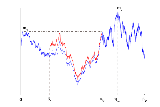
Figure 1: Sample path of $Z(t)$ generated by Algorithm 2.

The red curve represents the dominating process $U_{t}$. The process Z is not required to be simulated over the dashed-line.

To implement this idea, we need the following main components:

1. A sampling mechanism to generate $(t_{\zeta},\zeta,\beta)$. Here, $\beta$ is the first hitting time of the process $Z$ to a predetermined level, $\zeta$ is the maximum of the process over the interval $[\alpha,\beta]$, and $t_{\zeta}$ is the time at which the maximum occurs.

2. A testing procedure to check whether $Z(s)$ raises up level $m(\beta)=\displaystyle\sup_{0\leq u\leq\beta}Z_{u}$ at some time $s\geq\beta$.

In Section 5, we describe and analyze an algorithm to address i.). For ii.), we construct a constant drift Brownian motion $U^{\beta}=(U^{\beta}_{s}\colon s\geq\beta)$ dominating $Z(s)$. Let

$$U^{\beta}_{s}\triangleq d+Z(\beta)+B(s)-B(\beta)-(s-\beta)\cdot\bar{\gamma}.$$ (4.1)

By Assumption 3.2, we can conclude that $Z(s)\leq U_{s}^{\beta}$ for all $s\geq\beta$. If for one of $\beta_{k}$

$$U_{s}^{\beta_{k}}\leq m({\beta_{k}})=\displaystyle\sup_{0\leq u\leq\beta}Z_{u}$$

holds true for all $s\geq\beta_{k}$, then $m({\beta_{k}})$ is the global maximum of $Z$. Since $U_{s}^{\beta}$ is a constant drift Brownian motion, we can precisely characterize its first hitting time distribution (see Lemma 7.2). Hence, we can easily check whether $U^{\beta}$ hits level $m(\beta)$.

Below, we state the algorithm in detail. One can generate exact samples of $(v_{\infty},M(\infty))$ by setting $t=\infty$.

Algorithm 2 : Exact Sampling of $(v_{t},M(t),Y(t))$

1. Initialize $k=1$, $\zeta_{0}=\alpha_{0}=0$, $\eta_{t_{0}}=0$, and select parameters $c>1$ and $\epsilon>0$.

2. Generate a sample of $(t_{\zeta},\zeta,\beta_{k})$ by subroutine Subroutine 1: Exact Sampling of $(t_{\zeta},\displaystyle\sup_{t\leq\tilde{\tau}}Z(t),Z_{\tilde{\tau}})$, where

   $$\beta_{k}=\inf\{\Lambda^{-1}(t)\geq s\geq\epsilon+\alpha_{k}\colon Z(s)\leq m_{k}-cd\},$$ (4.2)

   $$\zeta_{k}=\displaystyle\max_{\alpha_{k}\leq s\leq\beta_{k}}Z(s),$$

   and $t_{\zeta}$ is the time at which maximum occurs.

3. -

   If $\zeta_{k}>m_{k}$, update $m_{k+1}=\zeta$ and $\eta_{t_{0}}\leftarrow t_{\zeta}$.

   -

   Otherwise, $m_{k+1}=m_{k}$.

4. Sample $\alpha_{k+1}=\inf\{s\geq\beta_{k}\colon U_{s}^{\beta_{k}}\geq m_{k}\}$; see Lemma 7.2.

5. If $\Lambda^{-1}(\alpha_{k+1})<t$, set $k\leftarrow k+1$, and repeat the procedure from Step 3.
                                                                                           Otherwise, terminate, and sample $Z(\Lambda(t))$ for $t<\infty$ conditional on $\alpha_{k+1}$.

6. Return $(\Lambda^{-1}(\eta_{t_{0}}),m_{k},Z(\Lambda(t)))$.

In Section 7, we show that

$$\mathbb{P}(\alpha_{k}=\infty)\geq 1-\exp(2\bar{\gamma}(c-1)d).$$

Therefore, the algorithm terminates in a finite number of iterations; call it $K$. The expectation of $K$ has an upper bound independent of $t$ even in the case $t=\infty$; see Theorem 7.1. Furthermore, it is straightforward to show that $\beta_{K}\leq L$; i.e, the length of the sample path generated by Algorithm 2 is less than $L$ which does not depend on $t$. Note that it is possible to determine whether $\Lambda^{-1}(\alpha_{k+1})<t$ or not in $\log(\alpha_{k+1})$, which is independent of $t$.

In the end, it is worth mentioning that we are not required to simulate the process over the entire interval $[0,\beta_{K}]$ to compute $\displaystyle\sup_{0\leq s\leq\beta_{K}}Z(s)$, since the maximum does not occur between $\beta_{k}$ and $\alpha_{k+1}$ for $k=1,\ldots,K-1$. In contrast, Algorithm 1, discussed in the previous section, requires generating the full path of the process (conditional on $L$) over $[0,L]$. Clearly, this is computationally more expensive than Algorithm 2.

In the next section, we discuss Step 2, generating exact samples for the maximum of $Z(t)$ over a finite interval.

5 Exact Sampling of Time-dependent Drift Brownian Motion

This section describes an exact method for sampling the unit-volatility time-dependent drift Brownian motion, and its maximum over a finite time interval, which can be employed as a subroutine in Step 2 of Algorithm 2. The method uses an acceptance/rejection mechanism similar to that of Beskos and Roberts (2005).

An acceptance/rejection scheme for exact simulation of state-dependent diffusions was developed for certain one-dimensional diffusions in Beskos and Roberts (2005). The generation of the acceptance indicator based on a thinning mechanism is proposed in Beskos et al. (2006). Furthermore, this scheme is extended to a wider class of diffusions in Chen and Huang (2013). Giesecke and Smelov (2013) generalized their method to jump-diffusions with state-dependent coefficients and jump intensity. Here, we develop a similar mechanism for time-dependent diffusions.

Recall that $Z=(Z(t):t\geq 0)$ is a Brownian motion with time-dependent drift $\gamma(t)$, so that the position at time $t$ is given by

$$Z(t)=B(t)+\int_{0}^{t}\gamma(s)ds.$$ (5.1)

The objective of this section is to generate an exact sample of the maximum of $Z$, before a fixed time $T_{f}$, or the first exiting time of the interval $(v,u)$, where $v<0$ and $u>0$. More formally, we generate an exact sample of

$$(t_{\zeta},\sup_{t\leq T_{f}\wedge\tau_{v,u}}Z(t),\tau_{v,u}),$$

where

$$\tau_{v,u}=\inf\{t\geq 0:Z(t)\notin(v,u)\}$$

is the first exit time of $Z$ from the interval $(v,u)$, and $t_{\zeta}$ is the time at which the maximum of $Z$ over $[0,T_{f}\wedge\tau_{v,u}]$ occurs. We can assume that $T_{f}$ is equal to infinity, in that case generating exact samples of the first hitting time is possible.

The key idea is to generate a candidate sample path of a standard Brownian motion and accept it as a sample path of the process $Z$ with the probability proportional to the likelihood ratio between the law of two processes. In Theorem 5.1, we calculate this likelihood ratio. Next, we construct a Bernoulli random variable $I$ for which $I=1$ with the acceptance probability proportional to the likelihood ratio, which indicates the acceptance of the candidate.

Let $\mathcal{F}=(\mathcal{F}_{t}:t\geq 0)$ be the filtration generated by the process $Z$ in (5.1), and $\bar{\tau}$ be a stopping time with respect to this filtration. Let $\mathbb{P}=\mathbb{P}(z;s,t)$ be the probability measure on the $\sigma$-field $\mathcal{F}_{\bar{\tau}\wedge t}$ induced by the path $\{Z({u\wedge\bar{\tau}})\colon s\leq u\leq t\wedge\bar{\tau}\}$. Theorem 5.1 provides a formula for the likelihood ratio between $\mathbb{P}$ and an equivalent measure $\mathbb{Q}=\mathbb{Q}(z;s,t)$ on $\mathcal{F}_{\bar{\tau}\wedge t}$ under which $\{Z({u\wedge\bar{\tau}})\colon s\leq u\leq t\wedge\bar{\tau}\}$ is a path of the standard Brownian motion stopped at $\bar{\tau}\wedge t$.

Theorem 5.1.

Let $Z(t)=B(t)+\int_{0}^{t}\gamma(s)ds$, $\gamma(t)$ be a continuously differentiable function, and $\bar{\tau}$ be a finite value stopping time with respect to the filtration $\mathcal{F}$. Then for any event $B\in\mathcal{F}_{\bar{\tau}\wedge t}$, we have

$$\frac{\mathbb{P}(B)}{\mathbb{Q}(B)}=\mathbb{E}^{\mathbb{Q}}\Big{[}\exp\left(\gamma(\bar{\tau}\wedge t)W^{\mathbb{Q}}_{\bar{\tau}\wedge t}-\frac{1}{2}\int_{s}^{\bar{\tau}\wedge t}\gamma^{2}(u)du-\int_{s}^{\bar{\tau}\wedge t}\gamma^{\prime}(u)W^{\mathbb{Q}}_{u}du\right)\Big{|}B\Big{]},$$ (5.2)

where $W_{t}^{\mathbb{Q}}$ is a $\mathbb{Q}$-Brownian motion starting at $W_{s}^{\mathbb{Q}}=Z(s)=z$.

Proof.

The proof is based on the Girsanov theorem, and Itô’s formula. Consider the supermartingale $M=(M(t)\colon{t\geq s})$ defined by

$$\mathcal{M}(t)=\exp\left(-\int_{s}^{t\wedge\bar{\tau}}\gamma(u)dB(u)-\frac{1}{2}\int_{s}^{t\wedge\bar{\tau}}\gamma(u)^{2}du\right)$$

Novikov’s condition guarantees that $M$ is a martingale. By the Girsanov theorem,

$$\frac{d\mathbb{Q}}{d\mathbb{P}}\Big{|}_{\mathcal{F}_{\bar{\tau}\wedge t}}=\mathcal{M}(t),$$

and under $\mathbb{Q}$ the process $W^{\mathbb{Q}}_{t\wedge\bar{\tau}}=z+B(t\wedge\bar{\tau})-B(s)+\int_{s}^{t\wedge\bar{\tau}}\gamma(s)ds=Z_{t\wedge\bar{\tau}}$ is a standard Brownian motion starting at $W_{s}=z$ and stopping at time $t\wedge\bar{\tau}$. By Itô’s formula and the differentiability assumption of $\gamma(t)$, we have

$$\gamma({t\wedge\bar{\tau}})W^{\mathbb{Q}}_{t\wedge\bar{\tau}}=\int_{s}^{t\wedge\bar{\tau}}\gamma(u)dW^{\mathbb{Q}}_{u}+\int_{s}^{t\wedge\bar{\tau}}\gamma^{\prime}(u)W^{\mathbb{Q}}_{u}du+\gamma(s)W_{s}.$$

Thus,

$$\frac{1}{\mathcal{M}_{t\wedge\bar{\tau}}} =\exp\Big{(}\int_{s}^{t\wedge\bar{\tau}}\gamma(u)dB(u)+\frac{1}{2}\int_{s}^{t\wedge\bar{\tau}}\gamma(u)^{2}du\Big{)}$$

$$=\exp\Big{(}\int_{s}^{t\wedge\bar{\tau}}\gamma(u)dW^{\mathbb{Q}}_{u}-\frac{1}{2}\int_{s}^{t\wedge\bar{\tau}}\gamma(u)^{2}du\Big{)}$$

$$=\exp\left(\gamma({t\wedge\bar{\tau}})W^{\mathbb{Q}}_{t\wedge\bar{\tau}}-\int_{s}^{{t\wedge\bar{\tau}}}\gamma^{\prime}(u)W^{\mathbb{Q}}_{u}du-\frac{1}{2}\int_{s}^{{t\wedge\bar{\tau}}}\gamma(u)^{2}du\right).$$

Therefore,

$$\frac{d\mathbb{P}}{d\mathbb{Q}}=\frac{1}{\mathcal{M}_{t\wedge\bar{\tau}}}=\exp\Big{(}\gamma({t\wedge\bar{\tau}})W^{\mathbb{Q}}_{t\wedge\bar{\tau}}-\int_{s}^{{t\wedge\bar{\tau}}}\gamma^{\prime}(u)W^{\mathbb{Q}}_{u}du-\frac{1}{2}\int_{s}^{{t\wedge\bar{\tau}}}\gamma(u)^{2}du\Big{)}$$

and

$$\mathbb{P}(B)=\mathbb{E}^{\mathbb{Q}}\left[\frac{1}{\mathcal{M}_{t\wedge\bar{\tau}}}I(\omega\in B)\right]=\mathbb{E}^{\mathbb{Q}}\left[\frac{1}{\mathcal{M}_{t\wedge\bar{\tau}}}\Big{|}B\right]\mathbb{Q}(B).$$

∎

To generate an exact sample path of $Z$, we follow the localization method developed by Chen and Huang (2013) and Giesecke and Smelov (2013). Suppose we have generated an exact sample of $(Z_{u}\ :\ u\leq s)$ for some random or fixed time $s<T_{f}\wedge\tau_{u,v}$. Define

$$\tau_{a}=\inf\{t\geq 0:|Z(t+s)-Z(s)|\geq a\},$$

where $a=\min\{|u-y|,\ |v-y|,\ \theta\}$ for some $\theta>0$. By following an acceptance/rejection procedure, we generate a sample path of

$$\Big{(}Z(t):s\leq u\leq s+(\tau_{a}\wedge\Delta)\Big{)}$$

for some parameter $\Delta$.

First, consider a sample path $\omega$ of $(W_{u}^{\mathbb{Q}}:s\leq u\leq s+\tau_{a}\wedge\Delta)$, where

$$\tau_{a}=\inf\{t>0:|W_{t+s}^{\mathbb{Q}}-W_{s}^{\mathbb{Q}}|\geq a\}.$$

For ease of exposition, we denote

$$W_{u}=W_{u+s}^{\mathbb{Q}}-W_{s}^{\mathbb{Q}}$$

for $0\leq u\leq\tau_{a}\wedge\Delta$, which is a standard Brownian motion under measure $\mathbb{Q}$. Now, given a sample path $\omega$ as a candidate, we construct a Bernoulli random variable $I$ with success probability proportional to

$$\mathbb{P}(I=1|\omega)\propto\frac{d\mathbb{P}(\omega)}{d\mathbb{Q}(\omega)}=\exp\Big{(}\gamma(\tau+s)W_{\tau}-\int_{0}^{\tau}\gamma^{\prime}(s+u)W_{u}du-\frac{1}{2}\int_{0}^{\tau}\gamma(u+s)^{2}du\Big{)},$$

where $\tau=\tau_{a}\wedge\Delta$. The candidate path $\omega$ is accepted as a sample path of $\Big{(}Z(t):s\leq t\leq s+(\Delta\wedge\tau_{a})\Big{)}$ if $I=1$; otherwise, we repeat the procedure.

The Bernoulli indicator $I$ can be constructed by sampling the jump times of a doubly-stochastic Possion process. The continuously differentiable assumption implies that $\gamma(\cdot)$ and $\gamma^{\prime}(\cdot)$ are bounded over the time interval $[s,s+\Delta]$. Let $m=\max_{t\in[s,s+\Delta]}|\gamma^{\prime}(t)|$, and $\tilde{m}=\max_{t\in[s,s+\Delta]}|\gamma(t)|$. Let

$$0\leq\phi_{t}=\gamma^{\prime}(s+t)W_{t}+ma\leq 2ma,$$

for every $0\leq t\leq\Delta$. Let $V$ be a doubly-stochastic Poisson process with intensity $\phi_{t}$ for $0\leq t\leq\Delta$. The required indicator can be generated by sampling the jump times of $V$ in $[0,\tau]$. The conditional probability that no jump occurs in the interval $[0,\tau]$ of the doubly-stochastic Poisson process $V$ is $\exp\left(\int_{0}^{\tau}\phi_{t}dt\right)$.

Let $E_{1}$ and $E_{2}$ be two independent exponential random variables with intensities

$$\lambda_{1}=\tilde{m}a-\gamma(\tau+s)W_{\tau}\geq 0$$

and

$$\lambda_{2}=-\frac{1}{2}\int_{s}^{\tau+s}\gamma^{2}(u)du+ma(\Delta-\tau)\geq 0.$$

The success probability of Bernoulli random $I$ can be defined by

$$\mathbb{P}(I=1|\omega)=\exp(-\int_{s}^{\tau+s}\phi_{u}du)\times\mathbb{P}(E_{1}>\tau)\times\mathbb{P}(E_{2}>\tau).$$

Observe that

$$\frac{d\mathbb{P}(\omega)}{d\mathbb{Q}(\omega)}={} \exp(-\int_{0}^{\tau}(\gamma^{\prime}(u+s)W_{u}du+ma)du\Big{)}$$

$$\times\exp\Big{(}\gamma(\tau+s)W_{\tau}-\tilde{m}a)$$

$$\times\exp\Big{(}-\frac{1}{2}\int_{s}^{\tau+s}\gamma^{2}(u)du+ma(\tau-\Delta)\Big{)}\exp(ma\Delta+\tilde{m}a)$$

$$={} \exp(-\int_{0}^{\tau}\phi_{u}du)\times\exp\Big{(}\gamma(\tau+s)W_{\tau}-\tilde{m}a)$$

$$\times\exp\Big{(}-\frac{1}{2}\int_{s}^{\tau+s}\gamma^{2}(u)du+ma(\tau-\Delta)\Big{)}\exp(ma\Delta+\tilde{m}a)$$

$$={} \mathbb{P}(I=1|\omega)\times\exp(ma\Delta+\tilde{m}a).$$ (5.3)

Generating exponential random variables $E_{1}$ and $E_{2}$ is straightforward. The intensity $\phi_{t}$ is bounded above by $2ma$, allowing us to simulate the event times of $V$ by thinning a Poisson process with intensity $2ma$. These properties facilitate generating the Bernoulli indicator for the acceptance test of a proposal skeleton.

More precisely, let $\kappa_{1},\kappa_{2},\ldots,\kappa_{b}<\tau$ be the jump times of a Poisson process with rate $2ma$, and $W_{\kappa_{i}}$ be the corresponding values of the candidate sample path for $i=1,\ldots,b$. Let $(U_{1},U_{2},\ldots,U_{b+2})$ be a sequence of $b+2$ uniform random variables. We accept the candidate path if

$$2maU_{i} >\gamma^{\prime}(\kappa_{i}+s)W_{\kappa_{i}}+ma\mbox{ \ \ \ \ \ \ \ \ \ for }1\leq i\leq b$$ (5.4)

$$U_{b+1} <\exp\Big{(}\gamma(\tau+s)W_{\tau}-\tilde{m}a\Big{)}$$

$$U_{b+2} <\exp\Big{(}\frac{-1}{2}\int_{s}^{\tau+s}\gamma^{2}(t)dt+am(\tau-\Delta)\Big{)}.$$

The sampling of an exit time $\tau_{a}$ for a Brownian motion $W^{\mathbb{Q}}$ is possible by following the method in Burq and Jones (2008). Moreover, in Chen and Huang (2013), it is shown that exact sampling of $W$ at a sequence of instances before $\tau$ is possible. Given a skeleton of the process at points $\kappa_{1},\kappa_{2},\ldots,\kappa_{b},\tau$, we can sample the maximum of the process over $[0,\tau]$. For every $i=1,\ldots,b$, observe that $\widetilde{W}_{t}=W_{t}+a$ is a Brownian meander for $\kappa_{i}\leq t\leq\kappa_{i+1}$ given that $t\leq\tau_{a}$. Maxmeander algorithm in Devroye (2010) generates exact samples of the maximum of the Brownian meander and the time at which the maximum occurs in constant expected time.

5.1 Summary of the Procedure

For the reader’s convenience, we summarize our basic algorithm for generating exact samples of the maximum of time-dependent BM over a finite time interval $[0,\tilde{\tau}]$, where $\tilde{\tau}=T_{f}\wedge\tau_{u,v}$. Let $\zeta=\displaystyle\sup_{0\leq t\leq\tilde{\tau}}Z(t)$ and $t_{\zeta}$ be the time at which the maximum occurs. The algorithm generates the triplet $(t_{\zeta},\zeta,Z_{\tilde{\tau}})$. This procedure can be used as a subroutine in Step 2 of Algorithm 2.

The initial conditions are $\zeta=0$, $t_{\zeta}=0$, $n=1$, $s_{1}=0$, and select $\theta>0$ and $\Delta<T_{f}$ (see Remark 5.2).

Subroutine 1: Exact Sampling of $(t_{\zeta},\displaystyle\sup_{t\leq\tilde{\tau}}Z(t),Z_{\tilde{\tau}})$

1. Set $a=\min\{|u-Z(s_{n})|,|v-Z(s_{n})|,\theta\}$.

2. Sample $\tau_{a}=\inf\{t\geq 0\ :\ |W_{t}|\geq a\}$; see Burq and Jones (2008).

3. Sample jump times $\kappa_{1},\kappa_{2},\ldots,\kappa_{b}<\tau_{a}\wedge\min\{T_{f}-s_{n},\Delta\}$ of a Poisson process with rate $2ma$. Set $\kappa_{b+1}=\tau_{a}\wedge\min\{T_{f}-s_{n},\Delta\}$.

4. Sample $W_{\kappa_{1}},W_{\kappa_{2}},\ldots,W_{\kappa_{b}},W_{\kappa_{b+1}},W_{\tau_{a}}$ conditional on $\tau_{a}$; see p. 11 of Chen and Huang (2013).

5. Accept/reject the proposal skeleton

   $$W_{\kappa_{1}},W_{\kappa_{2}},\ldots,W_{\kappa_{b}},W_{\kappa_{b+1},}W_{\tau_{a}}$$

   as a sample of the skeleton $(Z_{s_{n}+\kappa_{1}},Z_{s_{n}+\kappa_{2}},\ldots,Z_{s_{n}+\kappa_{b}},Z_{s_{n}+\kappa_{b+1}})$ if condition (5.4) holds.

   -

   If the proposal is rejected, go to Step 2.

   -

   If the proposal is accepted, set $s_{n+1}=s_{n}+\tau_{a}\wedge\min\{T-s_{n},\Delta\}$, and continue.

6. For $i=1,\ldots,b$, sample jointly $\mu_{i}=\sup_{\kappa_{i}\leq t\leq\kappa_{i+1}}W_{t}$ and $t_{\mu_{i}}$, the location of the maximum over $[\kappa_{i},\kappa_{i+1}]$ conditioned on $\tau_{a}$ as the maximum of a Brownian meander; see maxmeander algorithm in Devroye (2010).
   If $\zeta<\mu_{i}$, update $\zeta\leftarrow\mu_{i}$ and $t_{\zeta}\leftarrow t_{\mu_{i}}$.

7. If $s_{n+1}<T$, increase $n\leftarrow n+1$, and go to Step 1. Otherwise, stop and return $(t_{\zeta},\zeta,Z_{s_{n+1}})$.

Figure 2: Sample path of $Z(t)$ over $[s_{n},s_{n+1}]$ generated by Subroutine 1.

The running time of this algorithm can be bound by $\mathcal{O}(1/|\bar{\gamma}|)$. The following theorem shows this result.

Assumption 5.1.

Assume that

$$\frac{\theta^{2}}{\Delta}-\theta(\tilde{m}+\Delta m/2)\geq 2\log 2,$$

where $m=\sup_{u\geq 0}\gamma^{\prime}(u)$ and $\tilde{m}=\sup_{u\geq 0}\gamma(u)$.

Theorem 5.2.

Assume 3.1, 3.2, and 5.1 hold. For every $y>0$, let

$$\tau_{-y}=\inf\left\{t\geq 0\colon\ Z(t)\leq-y\right\}.$$

The running time of generating a skeleton of the sample path $\left(Z(t)\ :0\leq t\leq\tau_{-y}\right)$ by using the Subroutine 1 can be bounded by $\mathcal{O}\left(\frac{y+d+\theta}{|\bar{\gamma}|}\right)$ in expectation.

Proof.

Let $N$ be the number of time intervals $[s_{n},s_{n+1}]$ before the termination of the procedure. Also, assume that $\tau_{n}=s_{n+1}-s_{n}$ for $n=1,\ldots,N$. According to Lemma 5.3, we can show that $\mathbb{E}[R]$, the expectation of the running time of generating the skeleton of the sample path $\left(Z(t)\ :0\leq t\leq\tau_{-y}\right)$, is bounded by

$$\mathbb{E}[R]\leq cm\theta e^{m\theta\Delta+\tilde{m}\theta}(1+\Delta)\mathbb{E}[N]$$ (5.5)

for some constant $c$. By employing Lemma 5.4, we can bound $\mathbb{E}[N]$. We have

$$\mathbb{E}^{\mathbb{P}}[\tau_{-(y+\theta)}] \geq\mathbb{E}\left[\sum_{n=1}^{N}\tau_{n}\right]$$

$$\geq\mathbb{E}\left[\sum_{n=1}^{\infty}I(n\leq N)\mathbb{E}^{\mathbb{P}}[\tau_{n}|Z(s_{n})]\right]$$

$$\geq\mathbb{E}[N]\frac{\Delta}{4}.$$

The last inequality follows from Lemma 5.4. Therefore,

$$\mathbb{E}[N]\leq\frac{4}{\Delta}\mathbb{E}^{\mathbb{P}}[\tau_{-(y+\theta)}].$$

Let $\tilde{\tau}_{y+\theta}=\inf\{t\geq 0\colon B(t)-t\cdot\bar{\gamma}\leq y+\theta+d\}$ be the first hitting time of the dominating constant drift Brownian motion. It is clear that $\tau_{y+\theta}\leq\tilde{\tau}_{y+\theta+d}$ by Assumption (3.2). From optional sampling theorem (Karatzas and Shreve (1991, p. 19)), we can conclude that

$$\mathbb{E}^{\mathbb{P}}[\tau_{-(y+\theta)}]\leq\mathbb{E}^{\mathbb{P}}[\tilde{\tau}_{y+\theta+d}]$$

$$\leq\frac{y+\theta+d}{|\bar{\gamma}|}.$$

Therefore, we obtain

$$\mathbb{E}[N]\leq\frac{4(y+\theta+d)}{\Delta|\bar{\gamma}|}.$$ (5.6)

From inequalities (5.5) and (5.6), we conclude that

$$\mathbb{E}[R]\leq\frac{4(y+\theta+d)}{\Delta|\bar{\gamma}|}cm\theta e^{m\theta\Delta+\tilde{m}\theta}(1+\Delta).$$

Thus, the expected running time $\mathbb{E}R=\mathcal{O}\left(\frac{y+\theta+d}{|\bar{\gamma}|}\right)$. ∎

Remark 5.2.

In order to minimize the upper bound of the running time expectation, we can choose $\Delta=\frac{1}{m\theta}$ and select $\theta$ such that assumption (5.1) holds. A trial and error procedure might also help to choose the optimal $\Delta$ and $\theta$.

Lemma 5.3.

Assume that (5.1) holds. The expectation of the running time for generating the skeleton of $\left(Z(t)\ :s_{n}\leq t\leq s_{n+1}\right)$ is

$$\mathcal{O}(mae^{ma\Delta+\tilde{m}a}(1+\Delta)).$$

Proof.

The expectation of $b$, the number of events of the Poisson process with rate $2ma$ that occur in the time interval $[0,\tau_{a}\wedge\Delta]$ is

$$2ma\mathbb{E}^{Q}[\tau_{a}\wedge\Delta].$$

Sampling $W_{k_{i}}$ from a Brownian meander for each $i=1,\ldots,b+1$ in Step 3 is possible in a constant time. Therefore, the running time of generating a skeleton for each candidate sample path is

$$cma(1+\mathbb{E}^{Q}[\tau_{a}\wedge\Delta])$$

for some constant $c$. The probability of accepting each candidate sample path is

$$\mathbb{P}(I=1)=\exp(-ma\Delta-\tilde{m}).$$

Therefore, the expected number of candidate sample paths which are generated before acceptance occurs is $\exp(ma\Delta+\tilde{m})$. Thus, the expected running time to generate a skeleton for $\left(Z(t)\ :s_{n}\leq t\leq s_{n+1}\right)$ is at most

$$cmae^{ma\Delta+\tilde{m}a}(1+\mathbb{E}^{Q}[\tau_{a}\wedge\Delta])\leq cmae^{ma\Delta+\tilde{m}a}(1+\Delta)$$

for some constant $c$. ∎

Lemma 5.4.

Under assumption (5.1), we have

$$\mathbb{E}^{\mathbb{P}}[\tau_{n}\mid Z(s_{n})]\geq\Delta/4,$$

where $\tau_{n}=\inf\{t\geq 0\colon|Z(t+s_{n})-Z(s_{n})|\geq\theta\}$.

Proof.

By applying Theorem 5.1 and equality (5.3), we have

$$\mathbb{P}\left(\sup_{u\leq\Delta/2}|Z({u+s_{n}})-Z(s_{n})|\geq\theta\right) =\mathbb{E}^{Q}\left[I\left(\sup_{u\leq\Delta/2}|W_{u}|\geq\theta\right)\frac{\mathbb{P}(W\in d\omega)}{\mathbb{Q}(W\in d\omega)}\right]$$

$$\leq\exp(m\theta\Delta/2+\tilde{m}\theta)\mathbb{Q}\left(\sup_{u\leq\Delta/2}|W_{u}|\geq\theta\right)$$

$$\leq 2\exp(m\theta\Delta/2+\tilde{m}\theta-\theta^{2}/\Delta).$$

The last inequality follows from Doob’s martingale inequality. From Assumption (5.1), we can conclude that

$$\mathbb{P}(\tau_{n}\geq\Delta/2)=\mathbb{P}\left(\sup_{u\leq\Delta/2}|Z_{u+s_{n}}-Z(s_{n})|\leq\theta\right)\geq 1/2.$$

Therefore, we have

$$\mathbb{E}^{\mathbb{P}}[\tau_{n}|Z_{s_{n}}]\geq\frac{\Delta}{2}\mathbb{P}(\tau_{n}\geq\Delta/2)\geq\frac{\Delta}{4}.$$

∎

6 Exact Sampling of Time-dependent Drift Brownian Bridge

This section provides an exact method for sampling the maximum of a unit-volatility time-dependent drift Brownian bridge and the time at which this maximum occurs. We define a time-dependent drift Brownian bridge as a time-dependent Brownian motion given the prescribed values at the beginning and end of the process. Let $Z^{Br,r}=(Z(t)\colon 0\leq t\leq r)$ be a time-dependent drift Brownian bridge given $Z_{r}=y$. Recall that

$$Z(t)=B(t)+\int_{0}^{t}\gamma(u)du.$$

The objective of this section is to generate an exact sample of the maximum of

$$m(r)=\sup_{0\leq s\leq r}Z(s)$$

conditioned on $Z(r)=y$ and the time $\eta_{r}$ at which the maximum occurs. As we proposed in Algorithm 1, the procedure of sampling the joint variables $(\eta_{r},m(r))$ conditioned on $Z(r)=y$ can be employed as a subroutine to generate exact samples of ($\eta_{\infty},\sup_{t\geq 0}Z(t))$ as an alternative to Algorithm 2. Although, as we discussed earlier, Algorithm 2 is more efficient compared to this approach.

The procedure of generating exact samples of $(\eta_{r},m(r))$ conditioned on $Z(r)=y$ is similar to Subroutine 1, the exact sampling of the time-dependent Brownian motion. The main difference is that it uses a Brownian bridge rather than a standard Brownian motion as a candidate sample path. We accept this candidate as a sample path of $Z^{Br,r}$ with the probability proportional to the likelihood ratio between the law of two processes. Theorem 6.1 computes this likelihood ratio.

Similar to Subroutine 1  and following the localization method, the sample path of $Z^{Br,r}$ can be generated piece by piece over the time intervals $[s_{n},s_{n}+\Delta\wedge\tau_{a}]$ where

$$\tau_{a}=\inf\{t\geq 0\colon|Z(t+s_{n})-Z(s_{n})|\geq a\}$$

for appropriate parameters $a$ and $\Delta$ and given $(s_{n},Z(s_{n}))$.

Assuming $s_{n}+\Delta<r$, sampling $Z({s_{n}+\Delta})$ given $Z(r)=y$ is straightforward. Let

$$\tilde{x}=x-\int_{0}^{s_{n}+\Delta}\gamma(u)du,\tilde{y}=y-\int_{0}^{r}\gamma(u)du.$$

Observe that

$$\mathbb{P}\Big{(}Z({s_{n}+\Delta})\in dx\mid Z_{r}=y,Z(s_{n})\Big{)}=\mathbb{P}\Big{(}B({s_{n}+\Delta})\in d\tilde{x}\mid B({r})=\tilde{y},B({s_{n}})\Big{)},$$

which is the distribution of a standard Brownian bridge. Sampling of Brownian bridge is well known, and one can conveniently generate a sample of $Z({\Delta}+s_{n})$ given $Z_{r}=y$ and $Z(s_{n})$ . Therefore, it suffices to generate a sample of the process $Z^{Br,r}$ (and its maximum) over the time interval $[s_{n},s_{n}+\Delta\wedge\tau_{a}]$ given $Z(s_{n})$ and $Z({s_{n}+\Delta})$. By using time shifting, we can assume that $s_{n}=0$. Thus, the problem reduces to generating an exact sample of $(\eta_{\Delta},\sup_{0\leq t\leq\Delta}Z(t))$ given that $Z(\Delta)=x$.

The next theorem provides the likelihood ratio between the law of the process $Z^{Br,\Delta}$ and a standard Brownian bridge, which is used as the acceptance probability in the acceptance/rejection scheme.

Theorem 6.1.

Assume that $\gamma(s)$ is a continuously differentiable function, and let $\tau_{a}=\inf\{t\geq 0\colon|Z(t)-Z(0)|\geq a\}$. Then, for some constant $c_{1}$, we obtain

$$\frac{\mathbb{P}\Big{(}\ (Z(t))_{0\leq t\leq\Delta\wedge\tau_{a}}\in d\omega\Big{|}Z(\Delta)=x\ \Big{)}}{\mathbb{Q}\Big{(}(W_{t})_{0\leq t\leq\Delta\wedge\tau_{a}}\in d\omega\Big{|}W_{\Delta}=x\Big{)}}=c_{1}\mathbb{P}(I=1|\omega)\times e^{\psi(\omega)},$$ (6.1)

where

$$\psi(\omega)=\left\{\begin{array}[]{l l}0&\quad\text{if $\tau_{a}\geq\Delta$}\\ \frac{1}{2(\Delta-\tau_{a})}\left((x-\tilde{a})^{2}-(x-\tilde{a}-\int_{\tau_{a}}^{\Delta}\gamma(u)du)^{2}\right)&\quad\text{if $\tau_{a}<\Delta$,}\end{array}\right.$$

$\tilde{a}=Z({\tau_{a}})=\pm a$, and $\mathbb{P}(I=1|\omega)$ is defined in (5.3).

The proof is in the Appendix. Observe that

$$\psi(\omega)\leq\tilde{m}/2(x+a+\tilde{m}\Delta),$$

where $\tilde{m}=\sup_{0\leq t\leq\Delta}\gamma(t)$. Therefore, it is easily conceivable to construct a Bernoulli random variable with success probability proportional to $\exp(\psi(\omega))$.

Constructing the indicator $I$ is possible by modifying Steps 2, 3, and 4 in Subroutine 1. The main difference is in sampling $(\tau_{a},W_{\kappa_{1}},W_{\kappa_{2}},\ldots,W_{\kappa_{b}})$ conditional on $W_{\Delta}=x$, where $\kappa_{1},\kappa_{2},\ldots,\kappa_{b}<\tau_{a}\wedge\Delta$ are the jump times of a Poisson process with rate $2ma$. The procedure consists of:

1. Sample $(\tau_{a}\wedge\Delta,W_{\tau_{a}\wedge\Delta})$ given that $W_{\Delta}=x$.

2. Sample $\kappa_{1},\kappa_{2},\ldots,\kappa_{b}<\tau_{a}\wedge\Delta$, which are the jump times of a Poisson process with rate $2ma$.

3. Consider two different scenarios:

   -

   If $\tau_{a}\leq\Delta$, sample $W_{\kappa_{1}},W_{\kappa_{2}},\ldots,W_{\kappa_{b}}$ conditional on $(\tau_{a},W_{\tau_{a}})$.

   -

   If $\tau_{a}\leq\Delta$, sample $W_{\kappa_{1}},W_{\kappa_{2}},\ldots,W_{\kappa_{b}}$ conditional on $W_{\Delta}=x$ and $\tau_{a}\leq\Delta$.

The other steps of the procedure to generate a sample of $(\eta_{\Delta},m(\Delta))$ are exactly same as steps 5 and 6 in Subroutine 1.

Step $2^{\prime}$ is viable by using Theorem 6.2 in which we compute the likelihood ratio between distributions of the first hitting time of a Brownian bridge and a standard Brownian motion.

Theorem 6.2.

Let $\tau_{a}=\inf\{t\geq 0:|W_{t}|\geq a\}$ be the first hitting time of a standard Brownian motion $W$. Suppose that $r=\frac{|x|}{a}<1$, then we have

$$\mathbb{Q}(\tau_{a}\geq\Delta|W_{\Delta}=x)=\left(1-e^{-\frac{2(1-r)}{\Delta}}\right)\cdot p\left(0,1,\Delta,1-r\right),$$ (6.2)

where $p(s,x,t,y)$ is defined in (C.1). Moreover, for some constant $c_{2}$, we have

$$\frac{\mathbb{Q}\left(\tau_{a}\in dt,W_{\tau_{a}}=\tilde{a}|W_{\Delta}=x\right)}{\mathbb{Q}\left(\tau_{a}\in dt,W_{\tau_{a}}=\tilde{a}\right)}=c_{2}g\left(\frac{x-\tilde{a}}{\sqrt{\Delta-t}}\right)\leq\frac{c_{2}}{\sqrt{2\pi e}\cdot|a-|x||}$$ (6.3)

for every $t<\Delta$, where $g(\cdot)$ is the Gaussian function and $\tilde{a}=\pm a$.

The definition of the function $p(s,x,t,y)$ and the proof of the theorem can be found in the Appendix. This theorem facilitates step $2^{\prime}$ in the above procedure. If $|x|>a$, it is clear that $\tau_{a}<\Delta$. Suppose that $|x|<a$. Sampling the indicator $I(\tau_{a}\geq\Delta)$ is possible by generating two independent uniform random variables $U$ and $V$. If

$$U<p\left(0,1,\Delta,1-r\right)\mbox{ and\ }V<\left(1-e^{-\frac{2(1-r)}{\Delta}}\right)<1$$

hold true, we set $\tau_{a}\geq\Delta$, determining whether $U<p\left(0,1,\Delta,1-2r\right)$ is possible in finite time by Proposition 4.1 in Chen and Huang (2013).

The second part of Theorem 6.2 assists in generating a sample of $(\tau_{a},W_{\tau_{a}})$ conditional on the events $\tau_{a}<\Delta$ and $W_{\Delta}=x$. We can use the acceptance/rejection method. One can generate a sample of $(\tau_{a},W_{\tau_{a}})$ for a standard Brownian motion by following the proposed method in Burq and Jones (2008). According to equation (6.3), this sample might be accepted with the probability proportional to $g\left(\frac{x-\tilde{a}}{\sqrt{\Delta-t}}\right)$ as a sample of $(\tau_{a},W_{\tau_{a}})$ given that $\tau_{a}<\Delta$ and $W_{\Delta}=x$.

Step 2 of the above procedure is clear. Furthermore, if $\tau_{a}\leq\Delta$, generating $W_{\kappa_{1}},W_{\kappa_{2}},\ldots,W_{\kappa_{b}},W_{\tau_{a}}$ conditional on $\tau_{a}$ is possible by procedure (17) in Chen and Huang (2013). Now, we can assign $I=1$ if condition (5.4) holds.

In the rest of this part, we elaborate generating samples of $W$ at a sequence of instances $\kappa_{1},\kappa_{2},\ldots,\kappa_{b}<\tau_{a}\wedge\Delta$ conditioned on $W_{\Delta}=x$ and $\tau_{a}$ in the case that $\Delta<\tau_{a}$.

Let

$$\widetilde{W}_{t}=\begin{cases}1-\frac{1}{a}W_{\tau_{a}-ta^{2}}&\quad\text{if \ $W_{\tau_{a}=a}$ }\\ 1+\frac{1}{a}W_{\tau_{a}-ta^{2}}&\quad\text{if \ $W_{\tau_{a}=-a}$ }.\end{cases}$$

Thanks to the self-similarity and the time reverse properties of the Brownian motion, it is easy to verify that $\widetilde{W}=(\widetilde{W}_{t}\colon 0\leq t\leq\frac{\tau_{a}}{a^{2}})$ is a Brownian process given that $0\leq\widetilde{W}_{t_{1}}\leq 2$ and $\widetilde{W}_{t_{b+1}}=1-\frac{x}{a}$. Therefore, we are interested in generating samples of $\widetilde{W}$ at the sequence of instances

$$t_{0}=\frac{\tau_{a}}{a^{2}}\geq t_{1}\geq\ldots,\geq t_{b}\geq t_{b+1},$$

where $t_{i}=\frac{\tau_{a}-\kappa_{i}}{a^{2}}$ for $i=1,\ldots,b$.

Let $V=(V_{t}\colon t_{b+1}\leq t\leq t_{0})$ be a Brownian meander given that $V_{t_{b+1}}=1-\frac{x}{a}$ and $V_{t_{0}}=1$. The exact sampling of $(V_{t_{1}},\ldots,V_{t_{b}})$ is discussed in Devroye (2010, Section 6). One can generate a sample of the random vector $(V_{t_{1}},\ldots,V_{t_{b}})$ and accept that as a sample of $(\widetilde{W}_{t_{1}},\ldots,\widetilde{W}_{t_{b}})$ with the probability computed in Proposition 6.1. The acceptance decision can be determined by the method proposed in Chen and Huang (2013, Section 4.4).

Proposition 6.1.

For any $t_{0}\geq t_{1}\geq\ldots,\geq t_{b}\geq t_{b+1}$ and $0\leq y_{1},\ldots y_{b}\leq 2$, the joint conditional distribution of $(\widetilde{W}_{t_{1}},\ldots,\widetilde{W}_{t_{b}})$ has the following likelihood ratio with respect to $(V_{t_{1}},\ldots,V_{t_{b}})$:

$$\frac{\mathbb{Q}\left(\widetilde{W}_{t_{1}}\in dy_{1},\ldots,\widetilde{W}_{t_{b}}\in dy_{b}\Big{|}0\leq\widetilde{W}_{t}\leq 2,\widetilde{W}_{t_{b+1}}=y_{b+1},\widetilde{W}_{t_{0}}=1\right)}{\mathbb{Q}\left(V_{t_{1}}\in dy_{1},\ldots,V_{t_{b}}\in dy_{b}\Big{|}0\leq V_{t},V_{t_{b+1}}=y_{b+1},V_{t_{0}}=1\right)}=\tilde{c}\prod_{i=0}^{b}p(t_{i+1},y_{i+1};t_{i},y_{i}),$$

where $y_{b+1}=1-\frac{x}{a}$, $y_{0}=1$, and $\tilde{c}>0$ is a constant.

The proof of this proposition is similar to Theorem 4.2 in Chen and Huang (2013).

Given the skeleton $(\widetilde{W}_{\kappa_{1}},\ldots,\widetilde{W}_{\kappa_{b}},W_{\Delta})$, sampling $\sup_{0\leq t\leq\Delta}W_{t}$ and the location of maximum time is similar to Step 6 of Subroutine 1. It is sufficient to sample $(\mu_{i},t_{\mu_{i}})$ jointly, where $\mu_{i}=\sup_{\kappa_{i}\leq t\leq\kappa_{i+1}}W_{t}$, and $t_{\mu_{i}}$ is the location of the maximum over $[\kappa_{i},\kappa_{i+1}]$ conditional on $\tau_{a}$ as the maximum of a Brownian meander; see the maxmeander algorithm in Devroye (2010).

7 Analysis of the Algorithm 2

In this section, we analyze Algorithm 2 and show that the algorithm terminates in polynomial time. The running time of the algorithm is at most $\mathcal{O}(1/\bar{\gamma}^{2})$ for generating an exact sample of $(v_{t},M(t))$ which is independent of $t$. Therefore, the running time of the algorithm for generating an exact sample of triplet $(v_{t},M(t),Y(t))$ is at most $\mathcal{O}(1/\bar{\gamma}^{2})+\mathcal{O}(\log(t))$ in which $\mathcal{O}(\log(t))$ is the running time of reading the input and computing $Y(t)$ conditional on $(v_{t},M(t))$ .

The key idea here is constructing a constant drift Brownian motion, dominating $Z(s)$.

Lemma 7.1.

Let $m_{k}$ be the maximum of the process $Z(t)$ until time $\beta_{k}$, where $\beta_{k}$ is such that $Z({\beta_{k}})<\zeta_{k}-cd$. Then, $Z(t)<m_{k}$ for all $t<\alpha_{k+1}$. Specifically, if $\alpha_{k+1}=\infty$, then $m_{k}$ is the global maximum of $Z(t)$ for all $t\geq 0$.

Proof.

By Assumption (3.2), we have

$$Z(t) =Z({\beta_{k}})+B(t)-B({\beta_{k}})+\int_{\beta_{k}}^{t}\gamma(u)du$$

$$\leq Z({\beta_{k}})+B(t)-B({\beta_{k}})+d-(t-\beta_{k})\cdot\bar{\gamma}=U_{t}^{\beta_{k}}.$$

Observe that $U_{\beta_{k}}^{\beta_{k}}=Z({\beta_{k}})+d\leq m_{k}-(c-1)d$. Recall that

$$\alpha_{k+1}=\inf\{t\geq\beta_{k}\colon U_{t}\geq m_{k}\}.$$

Thus, we have $Z(t)<m_{k}$ for all $t<\alpha_{k+1}$. ∎

Generating exact samples of $\beta_{k+1}$ and $m_{k+1}$ is possible by Subroutine 1. Note that the process $U^{\beta_{k}}$ is a Brownian motion with constant drift. Therefore, we can easily sample the hitting time $\alpha_{k+1}$ based on the following lemma.

Lemma 7.2.

Let $x=m_{k}-U_{\beta_{k}}^{\beta_{k}}>0$. Then,

$$\mathbb{P}(\alpha_{k+1}=\infty|U_{\beta_{k}})=1-\exp(-2\bar{\gamma}x),$$

and

$$\mathbb{P}\Big{(}\alpha_{k+1}\leq t+\beta_{k}|U_{\beta_{k}}^{\beta_{k}},\alpha_{k+1}<\infty\Big{)}=\mathbb{P}\Big{(}IG\left(\frac{x}{|\bar{\gamma}|},x^{2}\right)\leq t\Big{)},$$ (7.1)

where $IG(\cdot,\cdot)$ denotes the inverse Gaussian-distribution with mean $\frac{x}{|\bar{\gamma}|}$ and shape parameter $x^{2}$.

Remark 7.3.

Draws from the inverse Gaussian distribution can be generated in a very efficient way; see the algorithm described in Devroye (1986, Chapter IV).

Proof.

By Assumption (3.2), $\bar{\gamma}>0$, and we have from Karatzas and Shreve (1991, p. 297) that

$$\mathbb{P}\Big{(}\alpha_{k+1}\geq T+\beta_{k}|U_{\beta_{k}}\Big{)}=\Phi\Big{(}\frac{x+\bar{\gamma}T}{\sqrt{T}}\Big{)}-\exp(-2\bar{\gamma}x)\Phi\Big{(}\frac{-x+\bar{\gamma}T}{\sqrt{T}}\Big{)}.$$

Therefore, $\mathbb{P}(\alpha_{k+1}=\infty|U_{\beta_{k}})=1-\exp(-2\bar{\gamma}x)$, and

$$\mathbb{P}\Big{(}\alpha_{k+1}\leq T+\beta_{k}|U_{\beta_{k}},\alpha_{k+1}<\infty\Big{)}=\exp(-2\bar{\gamma}x)\Phi\Big{(}\frac{-x+\bar{\gamma}T}{\sqrt{T}}\Big{)}+\Phi\Big{(}\frac{-x-\bar{\gamma}T}{\sqrt{T}}\Big{)},$$

which is the distribution of the inverse Gaussian distribution. ∎

As a result of these two lemmas, we can easily observe that the algorithm terminates in a finite number of iterations. The probability that the algorithm terminates in iteration $k$ (i.e. $\alpha_{k+1}=\infty$) is at least $1-\exp(-2\bar{\gamma}(c-1)d)$. Moreover, if $\alpha_{k+1}=\infty$, then $\zeta_{k}$ is the maximum of $Z(t)$ for all $t\geq 0$. So at each step $k$, the procedure is terminated with at least constant probability. Therefore, the algorithm terminates in finite time almost surely. We summarize this result in the following theorem.

Theorem 7.1.

For every $\bar{\gamma}>0$, Algorithm 2 terminates in finite time. Furthermore,The expected number of iterations is at most $(1-\exp{(-2(c-1)d\bar{\gamma})})^{-1}$, and the expected running time of generating an exact sample of $(v_{t},M(t))$ is $\mathcal{O}(1/\bar{\gamma}^{2})$ for every $t\in[0,\infty]$.

Proof.

It is clear that the running time of generating an exact sample of $(v_{t},M(t))$ is bounded for every $t\geq 0$ is bounded by the running time of generating an exact sample of $(v_{\infty},M(\infty))$. Therefore, we show the result for the recent case. Observe that

$$U_{\beta_{k}}^{\beta_{k}}=Z_{\beta_{k}}+d\leq m_{k}-(c-1)d.$$

Therefore, by Lemma 7.2, the probability that the algorithm terminates in the next step is

$$\mathbb{P}\Big{(}\alpha_{k+1}=\infty|U_{\beta_{k}}\Big{)}=1-\exp(2(m_{k}-U_{\beta_{k}})\bar{\gamma})\geq 1-\exp(2(c-1)d\bar{\gamma}).$$

Hence, the number of iterations before termination represented by $K$, is dominated by a geometric random variable. So we have

$$E[K]\leq(1-\exp{(-2(c-1)d\bar{\gamma})})^{-1}.$$

Given that $\alpha_{K}=\infty$, we have

$$Z(t)\leq U_{t}<m_{K}$$

for all $t>\beta_{K}$. Since $m_{K}$ is the maximum of the process until time $\beta_{k}$, we conclude that $\sup_{t\geq 0}Z(t)=m_{K}.$

According to Theorem 5.2, the expected running time of generating a sample of $\displaystyle\zeta_{k}=\sup_{\alpha_{k}\leq t<\beta_{k}}Z(t)$ by Subroutine 1 is $\mathcal{O}(1/|\bar{\gamma}|)$ for every $1\leq k\leq K$. Since,

$$E[K]=\mathcal{O}(1/|\bar{\gamma}|),$$

the expected running time of Algorithm 2 is $\mathcal{O}\left(1/\bar{\gamma}^{2}\right)$. ∎

In the end, it is worth mentioning that one can improve the performance of the algorithm by changing the update rule of $\beta_{k}$:

$$\beta_{k}=\inf\left\{t\geq\epsilon+\alpha_{k}\colon Z(t)\leq m^{\epsilon}_{k}-cd\right\},$$ (7.2)

where $m^{\epsilon}_{k}=\displaystyle\sup_{t\leq\epsilon+\alpha_{k-1}}Z(t)$. Here, $\epsilon$ is a parameter to guarantee that each step is not too short. Our simulation experiments show that choosing reasonable $\epsilon$ improves the running time.

8 Numerical Experiment

We illustrate the effectiveness and relative performance of the exact sampling method through the numerical experiment. We apply exact algorithm 2 to RBM with drift coefficient

$$\gamma(u)=\cos(2\pi u)-0.5.$$

In other words,

$$dX_{t}=(\cos(2\pi t)-0.5)dt+dB(t)+dL_{t}.$$ (8.1)

The drift coefficient $\gamma(u)=\cos(2\pi u)-0.5$ is a periodic function with period $1$, and

$$\bar{\gamma}=-\int_{0}^{1}\cos(2\pi u)-0.5du=0.5>0.$$

Therefore, Assumption 3.2 holds. Recall that

$$X(n)\Rightarrow M(\infty)=\sup_{t\geq 0}\Big{(}\int_{0}^{t}(\cos(2\pi u)-.5)du+B(t)\Big{)}.$$ (8.2)

In this experiment, we compare the discretization method and our exact algorithm for generating samples of $M(\infty)$. Conventional discretization techniques can only approximate samples of $M(\infty)$; the exact algorithm returns exact samples of $M(\infty)$.

8.1 Discretization Method

We compare the exact draws of our algorithms with the approximate ones of the simple discretization scheme. A naive approach to discretize (8.1) is given by

$$X_{t_{i+1}}=\max(X_{t_{i}}+\gamma(t_{i})(t_{i+1}-t_{i})+B(t_{i+1})-B(t_{i}),0),$$

where $t_{i}=i\delta$ for $i=1,2,\ldots$ and the step size $\delta>0$. However, Asmussen et al. (1995) shows that this discretization scheme is highly biased and the bias is at least of order $\delta^{1/2}$. As an alternative, we employ the discretization scheme for time-dependent RBM similar to Lépingle (1995). In Proposition A.1, we show that the bias of this scheme is of order $\delta^{2}$. Here, we quickly outline the discretization scheme. For time step $\delta>0$, define the piecewise constant drift Brownian motion $\hat{Z}^{\delta}=\{\hat{Z}^{\delta}(t)\}_{t\geq 0}$. Consider the discrete grid points $t_{i}=\delta i$ for $i=0,1,2,\ldots$. Let $\hat{Z}^{\delta}(t)=0$, and for $t_{i}\leq t\leq t_{i+1}$

$$\hat{Z}^{\delta}(t)\triangleq\hat{Z}^{\delta}(t_{i})+\gamma_{i}(t-t_{i})+B(t)-B(t_{i}),$$ (8.3)

where $\gamma_{i}=\frac{1}{\delta}\int_{t_{i}}^{t_{i+1}}\gamma(u)du$. The joint distribution of

$$\Big{(}\hat{Z}^{\delta}(t_{i+1}),\sup_{t_{i}\leq t\leq t_{i+1}}\hat{Z}^{\delta}(t)\Big{)}$$

given $\hat{Y}^{\delta}(t_{i})$ is known. Thus, the exact sampling of the process and its maximum over the grid points is possible. The details of the algorithm are given in Asmussen and Glynn (2007, p. 302). By choosing a large $T=t_{M}$ and sufficiently small $\delta$, the random variable $\displaystyle\sup_{0\leq t\leq t_{M}}\hat{Z}^{\delta}(t)$ approximates $M(\infty)$.

In Proposition A.1, we discuss how to allocate the computational budget of the discretization method between the number of time step $\delta$ and the number of trials. We show that for the first-order method of discretization, it is asymptotically optimal to increase the number of time steps proportional to the fourth root of the number of replications. However, the optimal constant of proportionality is not known.

8.2 Results

We generate samples of $M(\infty)$ defined in (8.2) using exact Algorithm 2 and the discretization scheme. For the discretization scheme, we use different increments $\delta$ and fixed time horizon $T=35$.

Table 1 presents the time required to get 200,000 draws from $M(\infty)$ for the exact algorithm and discretization scheme for different increments $\delta$. Moreover, the $p$-values of the Kolmogorov–Smirnov test are included, which compare the approximate samples of the Euler scheme with the exact sample for different increments $\delta$. The $p$-values indicate whether the samples are drawn from the same distribution or not.

Table 2 reports the comparison of the estimation of $\mathbb{E}[M(\infty)]$ by both methods. Motivated by Theorem A.1, the step size is set to $\delta=\frac{1}{5}N^{-\frac{1}{4}}$, where $N$ is the number of simulation trials. The fourth and fifth columns of the table show the estimation of $\mathbb{E}[M(\infty]$ and the $90\%$ confidence interval for different numbers of trials. The standard error (SE) is estimated as the sample standard deviation of the simulation output divided by the square root of the number of trials. The bias is given by the difference between the expectation of the estimator and the true value of $\mathbb{E}[M(\infty)]$. Bias of the estimator generated by the exact method is zero. Thus, the true value is estimated using $2$ million trials generated by the exact method. The bias of the discretization scheme is estimated by using 800,000 trails. The $8^{\mbox{th}}$ column of the table reports the root mean square error (RMSE) calculated by $\sqrt{\mbox{SE}^{2}+\mbox{Bias}^{2}}$. The last column shows the computational time required to generate different numbers of trials. Simulations were performed on a server with an Intel Core Duo 3.16 GHz processor and 4GB RAM.The code is written in MATLAB Version (R2011b).

It is remarkable that the exact algorithm is much more efficient than the discretization method. The bias is zero, the error is less, and even the algorithm improves the running time.

The convergence rates of the exact and discretization methods are compared in Figure 3. The exact method achieves an optimal convergence rate; RMSE of the estimator decreases at a rate of $\mathcal{O}(1/\sqrt{t})$, where $t$ is the computational budget. The convergence rate of the discretization scheme is $\mathcal{O}(t^{-2/5})$, confirming Theorem A.1. Since the convergence of the discretization scheme is slower, we can conclude that the discretization bias is significant.

Table 1: Comparing the samples generated by the discretization scheme and exact method by the Kolmogorov–Smirnov test.

	$\delta$	p-value	Time (Sec)
Discretization	$2^{-1}$	E-152	21
	$2^{-2}$	E-20	29
	$2^{-4}$	0.007	62
	$2^{-6}$	0.002	221
	$2^{-10}$	0.145	2305
	$2^{-12}$	0.231	11200
Exact Method	—	—	1305

Simulation Results of $\mathbb{E}[M(\infty]$ under Model (8.1). The p-values for the Kolmogorov–Smirnov test with null hypothesis that the exact and the corresponding approximate draws come from the same distribution.

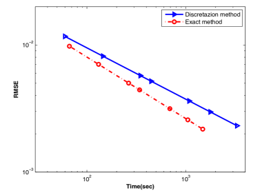
Figure 3: Convergence of the RMSEs computed by discretization and exact method.

The convergence rate of the exact scheme is $\mathcal{O}(t^{-1/2})$, and the convergence rate of discretization scheme is $\mathcal{O}(t^{-2/5})$.

Table 2: Simulation results of estimation $\mathbb{E}[M(\infty)]$ under the Model (8.1)

	Trials	Steps	Mean	90% CI	SE	Bias	RMSE	Time(sec)
Discretization	10000	2.00E-03	1.0519	[ 1.0356 , 1.0681 ]	9.89E-03	5.68E-03	1.14E-02	60
	20000	1.68E-03	1.0505	[ 1.0390 , 1.0620 ]	7.02E-03	4.28E-03	8.22E-03	145
	40000	1.41E-03	1.0490	[ 1.0409 , 1.0571 ]	4.95E-03	2.82E-03	5.70E-03	347
	50000	1.34E-03	1.0493	[ 1.0420 , 1.0565 ]	4.43E-03	3.09E-03	5.40E-03	446
	100000	1.12E-03	1.0484	[ 1.0433 , 1.0536 ]	3.12E-03	2.24E-03	3.85E-03	1081
	150000	1.02E-03	1.0470	[ 1.0428 , 1.0512 ]	2.56E-03	8.35E-04	2.69E-03	1769
	200000	9.46E-04	1.0470	[ 1.0434 , 1.0507 ]	2.21E-03	8.58E-04	2.37E-03	3290
Exact	10000	NA	1.0477	[ 1.0314 , 1.0639 ]	9.91E-03	0	9.91E-03	67
	20000	NA	1.0456	[ 1.0341 , 1.0571 ]	7.00E-03	0	7.00E-03	131
	40000	NA	1.0485	[ 1.0404 , 1.0566 ]	4.95E-03	0	4.95E-03	265
	50000	NA	1.0421	[ 1.0348 , 1.0494 ]	4.43E-03	0	4.43E-03	341
	100000	NA	1.0453	[ 1.0401 , 1.0504 ]	3.13E-03	0	3.13E-03	690
	150000	NA	1.0458	[ 1.0416 , 1.0500 ]	2.56E-03	0	2.56E-03	1049
	200000	NA	1.0468	[ 1.0432 , 1.0504 ]	2.21E-03	0	2.21E-03	1484

Appendix A Optimal Convergence Rate of Discretization Scheme

This appendix presents the optimal tradeoff between choosing the number of trials $N$ and time step $\delta$ in approximately generating samples by the discretization scheme discussed in Subsection 8.1. Suppose we want to compute $\alpha=\mathbb{E}[M(T)]$, where

$$M(T)=\sup_{0\leq t\leq T}B(t)+\int_{0}^{t}\gamma(u)du$$

by Monte Carlo simulation. However, we generate samples of

$$\hat{M}^{\delta}=\sup_{0\leq t\leq T}\hat{Z}^{\delta}(t)$$

in which $\hat{Z}^{\delta}(t)$ is defined by (8.3) using time steps of length $\delta$. As an estimator of $\alpha$, we compute

$$\hat{\alpha}(\delta,N)=\frac{1}{N}\sum_{j=1}^{N}\hat{M}^{\delta}_{j},$$

where $\hat{M}_{1}^{\delta},\ldots,\hat{M}_{N}^{\delta}$ is a sequence of i.i.d. copies of $\hat{M}^{\delta}$. The following assumption is required for Theorem A.1.

Assumption A.1.

Assume that

1. $\mathop{\rm var}\nolimits[\hat{M}^{\delta}]\rightarrow\mathop{\rm var}\nolimits[M(T)]$ as $\delta\downarrow 0$.

2. The function $\gamma(u)$ is continuously differentiable.

Theorem A.1.

Suppose $c$ is the computational budget to approximate $\alpha=\mathbb{E}M(T)$ by $\hat{\alpha}(\delta,N)$. Assume that A.1 holds. Then, it is asymptotically optimal to draw $N=\mathcal{O}(c^{\frac{4}{5}})$ trials and choose time step $\delta=\mathcal{O}(c^{\frac{-1}{5}})$ to minimize the root mean square error (RMSE) which gives RMSE at most $\mathcal{O}(c^{-\frac{2}{5}})$.

Proof.

By using Assumption A.1, we have

$$N\mathop{\rm var}\nolimits[\alpha(\delta,N)] =\frac{1}{N}\sum_{j=1}^{N}\mathop{\rm var}\nolimits[\hat{M}^{\delta}_{j}]$$

$$=\mathop{\rm var}\nolimits[\hat{M}^{\delta}]\rightarrow\mathop{\rm var}\nolimits[M(T)]$$ (A.1)

as $\delta\downarrow 0$. Note that

$$\mathbb{E}[(\hat{\alpha}(\delta,N)-\alpha)^{2}] =\mathop{\rm var}\nolimits[\alpha(\delta,N)]+(\alpha-\mathbb{E}[\hat{M}^{\delta}])^{2}$$

$$=\frac{1}{N}\mathop{\rm var}\nolimits[\hat{M}^{\delta}]+(\mathbb{E}[M(T)-\hat{M}^{\delta}])^{2}.$$

The first term is bound by $\mathcal{O}(\frac{1}{N})$ asymptotically. The second term can be bounded over each sample path. Observe that

$$|M(T)-\hat{M}^{\delta}| =\left|\sup_{0\leq t\leq T}Z(t)-\sup_{0\leq t\leq T}\hat{Z}^{\delta}(t)\right|$$

$$\leq\sup_{0\leq t\leq T}|Z(t)-\hat{Z}^{\delta}(t)|.$$

For every $t_{i}\leq t<t_{i+1}$ and $i=1,\ldots,{T/\delta}$, we obtain

$$|Z(t)-\hat{Z}^{\delta}(t)| =\left|B(t)+\int_{t_{i}}^{t}\gamma(u)du-\left(B(t)+\bar{\gamma}_{i}(t-t_{i})\right)\right|$$

$$\leq\left|\int_{t_{i}}^{t}\gamma(u)du-\bar{\gamma}_{i}(t-t_{i})\right|,$$

$$\leq m\delta^{2},$$

where $m=\sup_{0\leq t\leq T}\gamma^{\prime}(t)$ is constant. The last inequality is followed by Taylor’s theorem and the assumption that $\gamma(u)$ is continuously differentiable. Therefore,

$$\mathbb{E}[(M(T)-\hat{M}^{\delta})^{2}]\leq m^{2}\delta^{4}.$$ (A.2)

By combining (A.1) and (A.2), we have

$$\mathbb{E}[(\hat{\alpha}(\delta,N)-\alpha)^{2}]\leq m^{2}\delta^{4}+\frac{2}{N}\mathop{\rm var}\nolimits[M(T)]$$ (A.3)

for small enough $\delta$. Let $k$ be the constant time required to generate an exact sample of

$$O_{i}=\sup_{t_{i}\leq t\leq t_{i+1}}\hat{Z}^{\delta}(t).$$

The total computational budget required to draw $N$ independent samples of $\hat{M}^{\delta}=\max_{1\leq i\leq T/{\delta}}O_{i}$ is

$$c=k\cdot T/\delta\cdot(N+1).$$

Therefore, the right hand side of (A.3) can be minimized by selecting $N=\mathcal{O}(c^{\frac{4}{5}})$, and $\delta=\mathcal{O}(c^{-\frac{1}{5}})$. Moreover, we can conclude that the RMSE is $\mathcal{O}(c^{-\frac{2}{5}})$. ∎

Appendix B Proof of Theorem 6.1

Proof.

We consider two different scenarios. First, assume that $\omega\in\{\tau\leq\Delta\}$. Then, we have

$$\frac{\mathbb{P}\Big{(}\ (Z(t))_{0\leq t\leq\Delta\wedge\tau_{a}}\in d\omega\Big{|}Z(\Delta)=x\ \Big{)}}{\mathbb{Q}\Big{(}(W_{t})_{0\leq t\leq\Delta\wedge\tau_{a}}\in d\omega\Big{|}W_{\Delta}=x\Big{)}}={} \frac{\mathbb{P}\Big{(}\ (Z(t))_{0\leq t\leq\tau_{a}}\in d\omega,Z(\Delta)\in dx\ \Big{)}/\mathbb{P}(Z(\Delta)\in dx)}{\mathbb{Q}\Big{(}(W_{t})_{0\leq t\leq\tau_{a}}\in d\omega,W_{\Delta}\in dx\Big{)}/\mathbb{Q}(W_{\Delta}\in dx)}$$

$$={} \frac{\mathbb{P}\Big{(}\ (Z(t))_{0\leq t\leq\tau_{a}}\in d\omega\Big{)}\cdot\mathbb{P}(Z(\Delta)\in dx|Z(\tau_{a})=\tilde{a})}{\mathbb{Q}\Big{(}(W_{t})_{0\leq t\leq\tau_{a}}\in d\omega\Big{)}\cdot\mathbb{Q}(W_{\Delta}\in dx|W_{\tau_{a}}=\tilde{a})}$$

$$\times\frac{\mathbb{Q}(W_{\Delta}\in dx)}{\mathbb{P}(Z(\Delta)\in dx)}.$$

The last equality is obtained by applying the strong Markov property of Brownian motion. Observe that

$$\frac{\mathbb{P}(Z(\Delta)\in dx|Z(\tau_{a})=\tilde{a})}{\mathbb{Q}(W_{\Delta}\in dx|W_{\tau_{a}}=\tilde{a})} =\exp\left(\frac{1}{2(\Delta-\tau_{a})}\left(x-\tilde{a}-\int_{\tau_{a}}^{\Delta}\gamma(u)du\right)^{2}-(x-a)^{2}\right)$$

$$=\exp(\psi(\omega)).$$

From (5.3), we have

$$\frac{\mathbb{P}\Big{(}\ (Z(t))_{0\leq t\leq\tau_{a}}\in d\omega\Big{)}}{\mathbb{Q}\Big{(}(W_{t})_{0\leq t\leq\tau_{a}}\in d\omega\Big{)}}=\exp(ma\Delta+\tilde{m}a)\cdot\mathbb{P}(I=1|\omega).$$

Therefore, letting

$$c\triangleq\exp(ma\Delta+\tilde{m}a)\cdot\frac{\mathbb{Q}(W_{\Delta}\in dx)}{\mathbb{P}(Z(\Delta)\in dx)},$$

we can conclude the theorem. Similarly, In the case that $\omega\in\{\tau\geq\Delta\}$, we have

$$\frac{\mathbb{P}\Big{(}\ (Z(t))_{0\leq t\leq\Delta\wedge\tau_{a}}\in d\omega\Big{|}Z(\Delta)=x\ \Big{)}}{\mathbb{Q}\Big{(}(W_{t})_{0\leq t\leq\Delta\wedge\tau_{a}}\in d\omega\Big{|}W_{\Delta}=x\Big{)}} =\frac{\mathbb{P}\Big{(}\ (Z(t))_{0\leq t\leq\Delta}\in d\omega\Big{)}/\mathbb{P}(Z(\Delta)\in dx)}{\mathbb{Q}\Big{(}(W_{t})_{0\leq t\leq\Delta}\in d\omega\Big{)}/\mathbb{Q}(W_{\Delta}\in dx)}$$

$$=c\cdot\mathbb{P}(I=1|\omega).$$

∎

Appendix C Proof of Theorem 6.2

Definition C.1.

Denote $BB^{x\rightarrow y}_{u}$ to be the Brownian bridge from $x$ to $y$ on $[s,t]$. Let

$$p(s,x;t,y)\triangleq\mathbb{P}\left(0<BB^{x\rightarrow y}_{u}<2\mbox{, for all $u\in[s,t]$}\Big{|}0<BB^{x\rightarrow y}_{u}\mbox{, for all $u\in[s,t]$}\right).$$

In Chen and Huang (2013), it is shown that for any $s<t$ and $x,y\in[0,2]$, we have

$$p(s,x;t,y)=\frac{1-\sum_{j=1}^{\infty}(\theta_{j}-\vartheta_{j})}{1-\exp(-2xy/(t-s))},$$ (C.1)

where

$$\theta_{j}(s,x;t,y)\triangleq\exp\left(-\frac{2(2j-x)(2j-y)}{t-s}\right)+\exp\left(-\frac{2(2(j-1)+x)(2(j-1)+y)}{t-s}\right)$$

$$\vartheta_{j}(s,x;t,y)\triangleq\exp\left(-\frac{2j(4j+2(x-y))}{t-s}\right)+\exp\left(-\frac{2j(4j-2(x-y)}{t-s}\right).$$

Proof of Theorem 6.2. Let $\overline{BB}(t)=1-\frac{1}{a}W_{t}$ be a Brownian bridge conditional on $\overline{BB}(0)=1$ and $\overline{BB}(\Delta)=1-r$. Then, we have

$$\mathbb{Q}(\tau_{a}\geq\Delta) =\mathbb{Q}(-a\leq W_{t}\leq a|W_{\Delta}=x,W_{0}=0)$$

$$=\mathbb{Q}(0\leq\overline{BB}(t)\leq 2\mbox{, for all $0\leq t\leq\Delta$})$$

$$=p(0,1,\Delta,1-r)\mathbb{Q}\left(\overline{BB}(t)\geq 0\mbox{, for all $0\leq t\leq\Delta$}\right).$$

The last equality is concluded from p. 23 of Chen and Huang (2013). By using the distribution of the maximum of the Brownian bridge, we obtain

$$\mathbb{Q}\left(\overline{BB}(t)\geq 0\mbox{, for all $0\leq t\leq\Delta$}\right)=1-\exp\left(-\frac{2}{\Delta}(1-r)\right).$$

The second part of the theorem is straightforward.

References

- Asmussen (1992) Asmussen, S. (1992). Queueing simulation in heavy traffic. Mathematics of Operations Research, 17(1):84–111.
- Asmussen et al. (1995) Asmussen, S., Glynn, P., and Pitman, J. (1995). Discretization error in simulation of one-dimensional reflecting brownian motion. The Annals of Applied Probability, pages 875–896.
- Asmussen and Glynn (2007) Asmussen, S. and Glynn, P. W. (2007). Stochastic Simulation: Algorithms and Analysis. Springer, New York.
- Asmussen and Thorisson (1987) Asmussen, S. and Thorisson, H. (1987). A Markov chain approach to periodic queues. Journal of Applied Probability, 24(1):pp. 215–225.
- Bambos and Walrand (1989) Bambos, N. and Walrand, J. (1989). On queues with periodic inputs. Journal of Applied Probability, 26(2):pp. 381–389.
- Bass (2011) Bass, R. F. (2011). Stochastic Processes, volume 33. Cambridge University Press.
- Beskos et al. (2006) Beskos, A., Papaspiliopoulos, O., and Roberts, G. O. (2006). Retrospective exact simulation of diffusion sample paths with applications. Bernoulli, 12(6):1077–1098.
- Beskos and Roberts (2005) Beskos, A. and Roberts, G. O. (2005). Exact simulation of diffusions. The Annals of Applied Probability, 15(4):2422–2444.
- Burq and Jones (2008) Burq, Z. A. and Jones, O. D. (2008). Simulation of Brownian motion at first-passage times. Mathematics and Computers in Simulation, 77(1):64–71.
- Chen and Huang (2013) Chen, N. and Huang, Z. (2013). Localization and exact simulation of Brownian motion-driven stochastic differential equations. Mathematics of Operations Research, 38(3):591–616.
- Devroye (1986) Devroye, L. (1986). Non-Uniform Random Variate Generation. Springer, New York.
- Devroye (2010) Devroye, L. (2010). On exact simulation algorithms for some distributions related to Brownian motion and Brownian meanders. In Recent Developments in Applied Probability and Statistics, pages 1–35. Springer.
- Giesecke and Smelov (2013) Giesecke, K. and Smelov, D. (2013). Exact sampling of jump diffusions. Operations Research, 61(4):894–907.
- Harrison (1985) Harrison, J. M. (1985). Brownian Motion and Stochastic Flow Systems. Wiley, New York.
- Harrison and Lemoine (1977) Harrison, J. M. and Lemoine, A. J. (1977). Limit theorems for periodic queues. Journal of Applied Probability, 14(3):pp. 566–576.
- Heyman and Whitt (1984) Heyman, D. P. and Whitt, W. (1984). The asymptotic behavior of queues with time-varying arrival rates. Journal of Applied Probability, 21(1):pp. 143–156.
- Iglehart and Whitt (1970) Iglehart, D. L. and Whitt, W. (1970). Multiple channel queues in heavy traffic. I. Advances in Applied Probability, 2(1):150–177.
- Karatzas and Shreve (1991) Karatzas, I. and Shreve, S. (1991). Brownian Motion and Stochastic Calculus, volume 113. Springer Verlag, New York.
- Lépingle (1995) Lépingle, D. (1995). Euler scheme for reflected stochastic differential equations. Mathematics and Computers in Simulation, 38(1):119–126.
- Massey (1981) Massey, W. (1981). Non Stationary Queues. PhD thesis, Stanford University.
- Whitt (1989) Whitt, W. (1989). Planning queueing simulations. Management Science, 35(11):1341–1366.