Dirac quasinormal modes for a -dimensional Lifshitz black hole
Abstract
We study the quasinormal modes of fermionic perturbations for an asymptotically Lifshitz black hole in -dimensions with dynamical exponent and plane topology for the transverse section, and we find analytically and numerically the quasinormal modes for massless fermionic fields by using the improved asymptotic iteration method and the Horowitz-Hubeny method. The quasinormal frequencies are purely imaginary and negative, which guarantees the stability of these black holes under massless fermionic field perturbations. Remarkably, both numerical methods yield consistent results; i.e., both methods converge to the exact quasinormal frequencies; however, the improved asymptotic iteration method converges in a fewer number of iterations. Also, we find analytically the quasinormal modes for massive fermionic fields for the mode with lowest angular momentum. In this case, the quasinormal frequencies are purely imaginary and negative, which guarantees the stability of these black holes under fermionic field perturbations. Moreover, we show that the lowest quasinormal frequencies have real and imaginary parts for the mode with higher angular momentum by using the improved asymptotic iteration method.
I Introduction
The Lifshitz spacetimes have received great attention from the condensed matter point of view, i.e., the searching for gravity duals of Lifshitz fixed points due to the AdS/CFT correspondence for condensed matter physics and quantum chromodynamics Kachru:2008yh . From the quantum field theory point of view, there are many invariant scale theories of interest when studying such critical points. Such theories exhibit the anisotropic scale invariance , , with , where is the relative scale dimension of time and space, and they are of particular interest in studies of critical exponent theory and phase transitions. Systems with such a behavior appear, for instance, in the description of strongly correlated electrons. The importance of possessing a tool to study strongly-correlated condensed matter systems is beyond question, and consequently much attention has been focused on this area in recent years. Thermodynamically, it is difficult to compute conserved quantities for Lifshitz black holes; however, progress was made on the computation of mass and related thermodynamic quantities by using the ADT method Devecioglu:2010sf , Devecioglu:2011yi and the Euclidean action approach Gonzalez:2011nz ; Myung:2012cb . Also, phase transitions between Lifshitz black holes and other configurations with different asymptotes have been studied in Myung:2012xc . However, due to their different asymptotes these phases transitions do not occur.
An important property of black holes is their quasinormal modes (QNMs) and their quasinormal frequencies (QNFs) Regge:1957td ; Zerilli:1971wd ; Zerilli:1970se ; Kokkotas:1999bd ; Nollert:1999ji ; Konoplya:2011qq . The oscillation frequency of these modes is independent of the initial conditions and it only depends on the parameters of the black hole (mass, charge and angular momentum) and the fundamental constants (Newton constant and cosmological constant) that describe a black hole, just like the parameters that define the test field. The study of the QNFs gives information about the stability of black holes under matter fields that evolve perturbatively in their exterior region, without backreacting on the metric. In general, the oscillation frequencies are complex, where the real part represents the oscillation frequency and the imaginary part describes the rate at which this oscillation is damped, with the stability of the black hole being guaranteed if the imaginary part is negative. The QNFs have been calculated by means of numerical and analytical techniques, and the Mashhoon method, Chandrasekhar-Detweiler, WKB method, Frobenius method, method of continued fractions, Nollert and asymptotic iteration method (AIM) are some remarkably numerical methods. For a review see Konoplya:2011qq and the references therein. Generally, the Lifshitz black holes are stable under scalar perturbations, and the QNFs show the absence of a real part CuadrosMelgar:2011up ; Gonzalez:2012de ; Gonzalez:2012xc ; Myung:2012cb ; Becar:2012bj ; Giacomini:2012hg . In the context of black hole thermodynamics, the QNMs allow the quantum area spectrum of the black hole horizon to be studied CuadrosMelgar:2011up as well as the mass and the entropy spectrum.
On the other hand, the QNMs determine how fast a thermal state in the boundary theory will reach thermal equilibrium according to the AdS/CFT correspondence Maldacena:1997re , where the relaxation time of a thermal state of the boundary thermal theory is proportional to the inverse of the imaginary part of the QNFs of the dual gravity background, which was established due to the QNFs of the black hole being related to the poles of the retarded correlation function of the corresponding perturbations of the dual conformal field theory Birmingham:2001pj . Fermions on Lifshitz Background have been studied in Alishahiha:2012nm , by using the fermionic Green’s function in -dimensional Lifshitz spacetime with , also the authors considered a non-relativistic (mixed) boundary condition for fermions and showed that the spectrum has a flat band.
In this work, we will consider a matter distribution outside the horizon of the Lifshitz black hole in -dimensions with a plane transverse section and dynamical exponent . The matter is parameterized by a fermionic field, which we will perturb by assuming that there is no back reaction on the metric. We obtain analytically and numerically the QNFs for massless fermionic fields by using the improved AIM Cho:2009cj ; Cho:2011sf and the Horowitz-Hubeny method Horowitz:1999jd , and then we study their stability under fermionic perturbations. Also, we obtain analytically the QNFs of massive fermionic fields perturbations for the mode with lowest angular momentum and numerically the lowest QNF for the mode with higher angular momentum by using the improved AIM.
The paper is organized as follows. In Sec. II we give a brief review of the Lifshitz black holes considered in this work. In Sec. III we calculate the QNFs of fermionic perturbations for the -dimensional Lifshitz black hole with plane topology and . Finally, our conclusions are in Sec. IV.
II Lifshitz black hole
The Lifshitz spacetimes are described by the metrics
| (1) |
where represents a dimensional spatial vector, is the spacetime dimension and denotes the length scale in the geometry. As mentioned, this spacetime is interesting due to it being invariant under anisotropic scale transformation and represents the gravitational dual of strange metals Hartnoll:2009ns . If , then the spacetime is the usual anti-de Sitter metric in Poincaré coordinates. Furthermore, all scalar curvature invariants are constant and these spacetimes have a null curvature singularity at for , which can be seen by computing the tidal forces between infalling particles. This singularity is reached in finite proper time by infalling observers, so the spacetime is geodesically incomplete, Horowitz:2011gh . The metrics of the Lifshitz black hole asymptotically have the form (1). However, obtaining analytic solutions does not seem to be a trivial task, and therefore constructing finite temperature gravity duals requires the introduction of strange matter content the theoretical motivation of which is not clear. Another way of finding such a Lifshitz black hole solution is considering carefully-tuned higher-curvature modifications to the Hilbert-Einstein action, as in New Massive Gravity (NMG) in -dimensions or corrections to General Relativity. This has been done, for instance, in AyonBeato:2009nh ; Cai:2009ac ; AyonBeato:2010tm ; Dehghani:2010kd . A -dimensional topological black hole with a hyperbolic horizon and was found in Mann:2009yx and a set of analytical Lifshitz black holes in higher dimensions for arbitrary in Bertoldi:2009vn .
In this work we will consider a matter distribution outside the horizon of a black hole that asymptotically approaches the Lifshitz spacetime with Balasubramanian:2009rx , which is the solution for an action that corresponds to a black hole in a system with a strongly-coupled scalar, which is given by
| (2) |
where, is the Ricci scalar, is the cosmological constant, is a gauge field, is the field strength, , and
| (3) |
with
| (4) |
Note that the boundary of the spacetime is located at . Making the change of variable the metric can be put in the form
| (5) |
where
| (6) |
and by means of the change of coordinates the metric (5) becomes
| (7) |
In the next section, we will determine the QNFs by considering the Dirac equation in this background and by establishing the boundary conditions on the fermionic field at the horizon and at infinity.
III Fermionic quasinormal modes of a -dimensional Lifshitz Black Hole
A minimally coupled fermionic field to curvature in the background of a -dimensional Lifshitz Black Hole is given by the Dirac equation in curved space
| (8) |
where the covariant derivative is defined as
| (9) |
and the generators of the Lorentz group are
| (10) |
The gamma matrices in curved spacetime are defined by
| (11) |
where are the gamma matrices in a flat spacetime. In order to solve the Dirac equation, we use the diagonal vielbein
| (12) |
where denotes a vielbein for the flat base manifold . From the null torsion condition
| (13) |
we obtain the spin connection
| (14) |
Now, using the following representation of the gamma matrices
| (15) |
where are the Pauli matrices, and are the Dirac matrices in the base manifold , along with the following ansatz for the fermionic field
| (16) |
where is a two-component fermion. The following equations are thus obtained
| (17) | |||||
where is the eigenvalue of the Dirac operator in the base submanifold . In terms of the coordinate these equations can be written as
| (18) | |||||
where the prime denotes the derivative with respect to . In the following, we analyze two cases separately, one is the case and the other is . First, we will find analytically the QNFs for the mode with the lowest angular momentum, and for the modes with higher angular momentum we will obtain the QNFs analytically and numerically by using the improved AIM and the Horowitz-Hubeny approach.
III.1 Case
The following substitutions
| (19) |
in Eqs. (17) and the change of variables enable us to obtain the following equations
| (20) |
So, by decoupling from this system of equations and using
| (21) |
with
| (22) |
| (23) |
we obtain the hypergeometric equation for
| (24) |
and thus the solution is given by
| (25) |
which has three regular singular points at , and . Here, denotes the hypergeometric function and , are integration constants and the other constants are defined as
| (26) |
| (27) |
| (28) |
Now, imposing boundary conditions at the horizon, i.e., that there is only ingoing modes, implies that . Thus, the solution can be written as
| (29) |
On the other hand, using Kummer’s formula for hypergeometric functions, M. Abramowitz ,
| (30) | |||||
the behavior of the field at the boundary is given by
| (31) |
Imposing that the fermionic field vanishes at spatial infinity, we obtain for the conditions or , and for the conditions are or , where . Therefore, the following sets of quasinormal modes are obtained for
| (32) |
and for
| (33) |
Similarly, decoupling from the system of equations (III.1), we obtain another set of quasinormal frequencies, for
| (34) |
and for
| (35) |
So, the imaginary part of the QNFs is negative, which ensures the stability of the black hole under fermionic perturbations, at least for . Remarkably, it is known that the scalar QNFs of the BTZ black hole under Dirichlet boundary conditions permit to obtain only a set of QNFs, for positive masses of the scalar field. However, there is another set of QNFs for a range of imaginary masses which are allowed because the propagation of the scalar field is stable, according to the Breitenlohner-Freedman limit, Breitenlohner:1982bm ; Breitenlohner:1982jf . This set of QNFs, just as the former, can be obtained by requesting the flux to vanish at infinity, which are known as Neumann boundary conditions. It is worth mentioning that for fermionic perturbations there is no Breitenlohner-Freedman limit. However, it is possible to consider Neumann boundary conditions because Dirichlet boundary conditions would lead to the absence of QNFs for a range of masses, without a physical reason for this absence, Birmingham:2001pj . Here, we have considered Dirichlet boundary conditions at infinity and we have found that these boundary conditions yields two set of Dirac QNFs for all range of masses (positive and negative) of the fermionic field in analogy with Neumann boundary condition which yields two set of frequencies for the BTZ black hole.
III.2 Case
In this section we will compute the QNFs for the case . We will obtain analytical solutions for massless fermions, then we will employ two numerical methods as mentioned previously. Firstly, we will use the improved AIM and then we will compute some QNFs with the Horowitz-Hubeny method, and finally we will compare the results obtained with both methods.
III.2.1 Analytical solution
The change of variables in Eqs. (17) makes it possible to write the system of equations
| (36) | |||||
So, by decoupling this system of equations we can write the following equation for
| (37) |
where
| (38) | |||||
| (39) | |||||
and the variable is restricted to the range . For we get similar expressions changing for and for in the above equations. Firstly, in order to obtain an analytical solution we will consider the case . Thus, the functions and reduce to
| (40) | |||||
| (41) |
Now, using
| (42) |
with
| (43) |
| (44) |
we obtain the hypergeometric equation for
| (45) |
and thus the solution is given by
| (46) |
which has three regular singular points at , and . Here, denotes the hypergeometric function and , are integration constants and the other constants are defined as
| (47) |
| (48) |
| (49) |
Now, imposing boundary conditions at the horizon, i.e., that there is only ingoing modes, implies that . Thus, the solution can be written as
| (50) |
On the other hand, using Kummer’s formula for hypergeometric functions, Eq. (30), the behavior of the field at the boundary is given by
| (51) |
Imposing that the fermionic field vanishes at spatial infinity, we obtain the conditions or , where . Therefore, the following set of QNFs is obtained
| (52) |
Similarly, from the equation of we obtain another set of QNFs
| (53) |
Therefore, the imaginary part of the QNFs are negative, which ensures the stability of the black hole under fermionic perturbations.
III.2.2 Improved asymptotic iteration method
In this section we will employ the improved asymptotic iteration method, which is an improved version of the method proposed in Refs. Ciftci , Ciftci:2005xn . In order to apply this method, we must consider a fermionic field by incorporating its behavior at the horizon and at infinity. Accordingly, at the horizon, , the behavior of the fermionic field is given by the solution for the fields of Eq. (37) at the horizon, which is
| (54) |
| (55) |
So, in order to have only ingoing waves at the horizon, we impose , for and . Asymptotically, from Eq. (37), the fermionic field behaves as
| (56) |
So, in order to have a regular fermionic field at infinity we impose for . For the same expression is obtained. Therefore, taking into account these behaviors we define
| (57) |
| (58) |
Then, by inserting these fields in Eq. (37) we obtain the homogeneous linear second-order differential equation for the function
| (59) |
where for
| (60) | |||||
| (61) | |||||
and for we get
| (62) | |||||
| (63) | |||||
Then, in order to implement the improved AIM it is necessary to differentiate Eq. (59) times with respect to , which yields the following equation:
| (64) |
where
| (65) |
| (66) |
Then, by expanding the and in a Taylor series around the point, , at which the improved AIM is performed
| (67) |
| (68) |
where the and are the Taylor coefficients of and , respectively, and by replacing the above expansion in Eqs. (65) and (66) the following set of recursion relations for the coefficients is obtained:
| (69) |
| (70) |
In this manner, the authors of the improved AIM have avoided the derivatives that contain the AIM in Cho:2009cj ; Cho:2011sf , and the quantization conditions, which is equivalent to imposing a termination to the number of iterations Barakat:2006ki , which is given by
| (71) |
We solve this numerically to find the QNFs. In Tables 1 and 2, we show the lowest QNFs, for a massless fermionic field with and , and . Additionally, in Table 3 we show the lowest QNFs for the fermionic fields with different values of the mass. In this case, the lowest QNFs have real and imaginary parts. The results in Table 1 refer to and in Table 2 to . It is worth mentioning that a number of 25 iterations was employed for the improved AIM method. We can appreciate that the imaginary part of the QNFs are negative, which ensures the stability of the -dimensional Lifshitz Black Hole under fermionic perturbations and that for the fermionic massless field the QNFs are purely imaginary.
III.2.3 Horowitz-Hubeny method
In this section we will employ the Horowitz-Hubeny method to evaluate some QNFs for massless fermionic field (for instance, see Cai:2010tr ; Jing:2005ux ). In this way, we can compare both methods in order to check the results obtained in this work employing different methods. Thus, by decoupling the system of Eqs. (18) we obtain the following equations for the fields:
| (72) |
| (73) |
Then, by using the Tortoise coordinate
| (74) |
and also employing
| (75) |
it is possible to write (72) and (73) as a Schrödinger-like equation
| (76) |
where the effective potential is given by
| (77) |
Here, the sign refers to two sets of QNMs associated with and , respectively. Thus, by performing the redefinition
| (78) |
we get
| (79) |
and with the change of coordinates , this expression becomes
| (80) |
where the functions , and are defined by
| (81) |
| (82) |
| (83) |
and . The functions , and are fourth-degree polynomials. Now, we expand the polynomials around the horizon in the form and in a similar way for and . Also, we expand the wave function as
| (84) |
Now, in order to find the exponent we have that near the event horizon the wave function behaves as . So, by substituting this in Eq. (80) we get
| (85) |
where the solutions of this algebraic equation are and for the minus sign in the effective potential. The boundary condition, i.e. that near the event horizon there are only ingoing modes, imposes that . For the plus sign the solution is . Finally, by substituting , , and in (80) we find the following recursion relation
| (86) |
with
| (87) |
Imposing the Dirichlet boundary condition at implies that
| (88) |
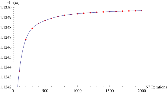
Therefore, we can obtain the QNFs solving this equation numerically. In Tables 4 and 5, we show the lowest QNFs, for massless fermionic field with and , and . The results in Table 4 refer to the negative sign in the effective potential () and in Table 5 to the positive sign () where we can appreciate that the imaginary part of the quasinormal frequencies are negative, which ensures the stability of the black hole under fermionic perturbations. It is worth mentioning that a number of iterations was employed for the Horowitz-Hubeny method, i.e. we take up to terms in the sum. The convergence of the quasinormal frequency with the number of iterations is shown in Figure (1), for , and . It is also worth mentioning that at 2000 iterations the difference between two consecutive frequencies is less than . Moreover, the QNFs that we have found via the Horowitz-Hubeny approach are similar to the QNFs that we found via the improved AIM, previously.
IV Conclusions
In this work we have calculated the QNFs of massless fermionic perturbations for the -dimensional Lifshitz black hole with a plane topology and dynamical exponent . It is known that the boundary conditions depend on the asymptotic behavior of spacetime. For asymptotically AdS spacetimes the potential diverges and thus the field must be null at infinity (Dirichlet boundary conditions) or the flux must vanish at infinity, which are known as Neumann boundary conditions. Here, as the black hole is asymptotically Lifshitz and the potential diverges at the boundary, we have considered that the fermionic fields will be null at infinity (Dirichlet boundary conditions) and that there are only ingoing modes at the horizon, and we have obtained analytical and numerical results using the improved AIM and the Horowit-Hubeny method, and we have found that the QNFs for the massless fermionic field are purely imaginary and negative, which ensures the stability of the black hole under massless fermionic perturbations. Remarkably, both numerical methods yield consistent results; i.e., both methods converge to the exact QNFs; however, the improved AIM converges in a fewer number of iterations.
Also, we have found analytically the QNFs for massive fermionic fields for the mode with lowest angular momentum, being the QNFs purely imaginary and negative, which guarantees the stability of these black holes under fermionic fields perturbations. Interestingly, in this case we obtain two sets of Dirac QNFs that cover all the range of mass (positive and negative) of the fermionic field in analogy with Neumann boundary condition which yields two set of modes in the BTZ black hole. On the other hand, we have shown that the lowest QNFs for massive fermionic fields for the mode with higher angular momentum, have a real and imaginary parts, by using the improved AIM.
Acknowledgments
P.G. would like to thank Felipe Leyton for valuable discussions and comments on numerical methods. This work was funded by the Comisión Nacional de Investigación Científica y Tecnológica through FONDECYT Grant 11121148 (YV, MC) and also partially funded by Dirección de investigación, Universidad de La Frontera (MC). The authors also thank partial support by NLHCP (ECM-02) at CMCC UFRO. P.G. and Y.V. acknowledge the hospitality of the Universidad de La Frontera where part of this work was undertaken.
References
- (1) S. Kachru, X. Liu and M. Mulligan, Phys. Rev. D 78, 106005 (2008) [arXiv:0808.1725 [hep-th]].
- (2) D. O. Devecioglu and O. Sarioglu, Phys. Rev. D 83 (2011) 021503 [arXiv:1010.1711 [hep-th]].
- (3) D. O. Devecioglu and O. Sarioglu, Phys. Rev. D 83 (2011) 124041 [arXiv:1103.1993 [hep-th]].
- (4) H. A. Gonzalez, D. Tempo and R. Troncoso, JHEP 1111 (2011) 066 [arXiv:1107.3647 [hep-th]].
- (5) Y. S. Myung and T. Moon, Phys. Rev. D 86 (2012) 024006 [arXiv:1204.2116 [hep-th]].
- (6) Y. S. Myung, Eur. Phys. J. C 72 (2012) 2116 [arXiv:1203.1367 [hep-th]].
- (7) T. Regge and J. A. Wheeler, Phys. Rev. 108, 1063 (1957).
- (8) F. J. Zerilli, Phys. Rev. D 2, 2141 (1970).
- (9) F. J. Zerilli, Phys. Rev. Lett. 24, 737 (1970).
- (10) K. D. Kokkotas and B. G. Schmidt, Living Rev. Rel. 2, 2 (1999) [gr-qc/9909058].
- (11) H. -P. Nollert, Class. Quant. Grav. 16, R159 (1999).
- (12) R. A. Konoplya and A. Zhidenko, Rev. Mod. Phys. 83, 793 (2011) [arXiv:1102.4014 [gr-qc]].
- (13) B. Cuadros-Melgar, J. de Oliveira and C. E. Pellicer, Phys. Rev. D 85, 024014 (2012) [arXiv:1110.4856 [hep-th]].
- (14) P. A. Gonzalez, J. Saavedra and Y. Vasquez, Int. J. Mod. Phys. D 21, 1250054 (2012) [arXiv:1201.4521 [gr-qc]].
- (15) P. A. Gonzalez, F. Moncada and Y. Vasquez, Eur. Phys. J. C 72, 2255 (2012) [arXiv:1205.0582 [gr-qc]].
- (16) R. Becar, P. A. Gonzalez and Y. Vasquez, Int. J. Mod. Phys. D 22, 1350007 (2013) [arXiv:1210.7561 [gr-qc]].
- (17) A. Giacomini, G. Giribet, M. Leston, J. Oliva and S. Ray, Phys. Rev. D 85 (2012) 124001 [arXiv:1203.0582 [hep-th]].
- (18) J. M. Maldacena, Adv. Theor. Math. Phys. 2, 231 (1998) [hep-th/9711200].
- (19) D. Birmingham, I. Sachs and S. N. Solodukhin, Phys. Rev. Lett. 88, 151301 (2002) [hep-th/0112055].
- (20) M. Alishahiha, M. R. Mohammadi Mozaffar and A. Mollabashi, Phys. Rev. D 86 (2012) 026002 [arXiv:1201.1764 [hep-th]].
- (21) H. T. Cho, A. S. Cornell, J. Doukas and W. Naylor, Class. Quant. Grav. 27 (2010) 155004 [arXiv:0912.2740 [gr-qc]].
- (22) H. T. Cho, A. S. Cornell, J. Doukas, T. R. Huang and W. Naylor, Adv. Math. Phys. 2012 (2012) 281705 [arXiv:1111.5024 [gr-qc]].
- (23) G. T. Horowitz and V. E. Hubeny, Phys. Rev. D 62, 024027 (2000) [hep-th/9909056].
- (24) S. A. Hartnoll, J. Polchinski, E. Silverstein and D. Tong, JHEP 1004, 120 (2010) [arXiv:0912.1061 [hep-th]].
- (25) G. T. Horowitz and B. Way, Phys. Rev. D 85 (2012) 046008 [arXiv:1111.1243 [hep-th]].
- (26) E. Ayon-Beato, A. Garbarz, G. Giribet and M. Hassaine, Phys. Rev. D 80 (2009) 104029 [arXiv:0909.1347 [hep-th]].
- (27) R. -G. Cai, Y. Liu and Y. -W. Sun, JHEP 0910 (2009) 080 [arXiv:0909.2807 [hep-th]].
- (28) E. Ayon-Beato, A. Garbarz, G. Giribet and M. Hassaine, JHEP 1004 (2010) 030 [arXiv:1001.2361 [hep-th]].
- (29) M. H. Dehghani and R. B. Mann, JHEP 1007 (2010) 019 [arXiv:1004.4397 [hep-th]].
- (30) R. B. Mann, JHEP 0906 (2009) 075 [arXiv:0905.1136 [hep-th]].
- (31) G. Bertoldi, B. A. Burrington and A. Peet, Phys. Rev. D 80 (2009) 126003 [arXiv:0905.3183 [hep-th]].
- (32) K. Balasubramanian, J. McGreevy, Phys. Rev. D80, 104039 (2009). [arXiv:0909.0263 [hep-th]].
- (33) M. Abramowitz and A. Stegun, Handbook of Mathematical functions, (Dover publications, New York, 1970).
- (34) P. Breitenlohner and D. Z. Freedman, Phys. Lett. B 115, 197 (1982).
- (35) P. Breitenlohner and D. Z. Freedman, Annals Phys. 144, 249 (1982).
- (36) H. Ciftci, R. L. Hall, and N. Saad, Journal of Physics A, vol. 36, no. 47, pp. 11807�11816, 2003.
- (37) H. Ciftci, R. L. Hall and N. Saad, Phys. Lett. A 340 (2005) 388.
- (38) T. Barakat, Int. J. Mod. Phys. A 21 (2006) 4127.
- (39) R. -G. Cai, Z. -Y. Nie, B. Wang and H. -Q. Zhang, arXiv:1005.1233 [gr-qc].
- (40) J. -l. Jing, gr-qc/0502010.