Complex short pulse and coupled complex short pulse equations

Abstract

In the present paper, we propose a complex short pulse equation and a coupled complex short equation to describe ultra-short pulse propagation in optical fibers. They are integrable due to the existence of Lax pairs and infinite number of conservation laws. Furthermore, we find their multi-soliton solutions in terms of pfaffians by virtue of Hirota’s bilinear method. One- and two-soliton solutions are investigated in details, showing favorable properties in modeling ulta-short pulses with a few optical cycles. Especially, same as the coupled nonlinear Schrödinger equation, there is an interesting phenomenon of energy redistribution in soliton interactions. It is expected that, for the ultra-short pulses, the complex and coupled complex short pulses equation will play the same roles as the nonlinear Schrödinger equation and coupled nonlinear Schrödinger equation.

Keywords: Complex short pulse equation; Coupled complex short pulse equation; Hirota bilinear method; Pfaffian; Envelope soliton; Soliton interaction.

1 Introduction

The nonlinear Schrödinger (NLS) equation, as one of the universal equations that describe the evolution of slowly varying packets of quasi-monochromatic waves in weakly nonlinear dispersive media, has been very successful in many applications such as nonlinear optics and water waves [1, 2, 3, 4]. The NLS equation is integrable, which can be solved by the inverse scattering transform [5].

However, in the regime of ultra-short pulses where the width of optical pulse is in the order of femtosecond ($10^{-15}$ s), the NLS equation becomes less accurate [6]. Description of ultra-short processes requires a modification of standard slow varying envelope models based on the NLS equation. There are usually two approaches to meet this requirement in the literature. The first one is to add several higher-order dispersive terms to get higher-order NLS equation [2]. The second one is to construct a suitable fit to the frequency-dependent dielectric constant $\epsilon(\omega)$ in the desired spectral range. Several models have been proposed by this approach including the short-pulse (SP) equation [7, 8, 9, 10].

Recently, Schäfer and Wayne derived a so-called short pulse (SP) equation [7]

$$u_{xt}=u+\frac{1}{6}\left(u^{3}\right)_{xx}\,,$$ (1)

to describe the propagation of ultra-short optical pulses in nonlinear media. Here, $u=u(x,t)$ is a real-valued function, representing the magnitude of the electric field, the subscripts $t$ and $x$ denote partial differentiation. Apart from the context of nonlinear optics, the SP equation has also been derived as an integrable differential equation associated with pseudospherical surfaces [11]. The SP equation has been shown to be completely integrable [11, 12, 13, 14, 15]. The periodic and soliton solutions of the SP equation were found in [16, 17, 18]. The connection between the SP equation and the sine-Gordon equation through the hodograph transformation was clarified, and then the $N$-soliton solutions including multi-loop and multi-breather ones were given in [19, 20] by using the Hirota bilinear method [21]. The integrable discretization of the SP equation was studied in [22], the geometric interpretation of the SP equation, as well as its integrable discretization, was given in [23]. The higher-order corrections to the SP equation was studied in [24] most recently.

Similar to the case of the NLS equation [25], it is necessary to consider its two-component or multi-component generalizations of the SP equation for describing the effects of polarization or anisotropy. As a matter of fact, several integrable coupled short pulse have been proposed in the literature [26, 27, 28, 29, 30, 31]. Most recently, the bi-Hamiltonian structures for the above two-component SP equations were obtained by Brunelli [32].

In the present paper, we propose and study a complex short pulse (CSP) equation

$$q_{xt}+q+\frac{1}{2}\left(|q|^{2}q_{x}\right)_{x}=0\,,$$ (2)

and its two-component generalization

$$q_{1,xt}+q_{1}+\frac{1}{2}\left((|q_{1}|^{2}+|q_{2}|^{2})q_{1,x}\right)_{x}=0\,,$$ (3)

$$q_{2,xt}+q_{2}+\frac{1}{2}\left((|q_{1}|^{2}+|q_{2}|^{2})q_{2,x}\right)_{x}=0\,.$$ (4)

As will be revealed in the present paper, both the CSP equation and its two-component generalization are integrable guaranteed by the existence of Lax pairs and infinite number of conservation laws. They have $N$-soliton solutions which can be constructed via Hirota’s bilinear method.

The outline of the present paper is organized as follows. In section 2, we derive the CSP equation and coupled complex short pulse (CCSP) equation from the physical context. In section 3, by providing the Lax pairs, the integrability of the proposed two equations are confirmed, and further, the conservation laws, both local and nonlocal ones, are investigated. Then $N$-soliton solutions to both the CSP and CCSP equations are constructed in terms of pfaffians by Hirota’s bilinear method in section 4. In section 5, soliton-interaction for coupled complex short pulse equation is investigated in details, which shows rich phenomena similar to the coupled nonlinear Schrödinger equatoin. In particular, they may undergo either elastic or inelastic collision depending on the initial conditions. For inelastic collisions, there is an energy exchange between solitons, which can allow the generation or vanishing of soliton. The dynamics is more richer in compared with the single component case. The paper is concluded by comments and remarks in section 6.

2 The derivation of the complex short pulse and coupled complex short pulse equations

In this section, following the procedure in [2, 7], we derive the complex short pulse equation (2) and its two-component generalization that governs the propagation of ultra short pulse packet along optical fibers.

2.1 The complex short pulse equation

We start with a wave equation for electric field

$$\nabla^{2}\mathbf{E}-\frac{1}{c^{2}}\mathbf{E}_{tt}=\mu_{0}\mathbf{P}_{tt}\,,$$ (5)

originated from the Maxwell equation. Here $\mathbf{E}(\mathbf{r},t)$ and $\mathbf{P}(\mathbf{r},t)$ represent the electric field and the induced polarization, respectively, $\mu_{0}$ is the vacuum permeability, $c$ is the speed of light in vacuum. If we assume the local medium response and only the third-order nonlinear effects governed by $\chi^{(3)}$, the induced polarization consists of two parts, $\mathbf{P}(\mathbf{r},t)=\mathbf{P}_{L}(\mathbf{r},t)+\mathbf{P}_{NL}(\mathbf{r},t)$, where the linear part

$$\mathbf{P}_{L}(\mathbf{r},t)=\epsilon_{0}\int_{-\infty}^{\infty}\chi^{(1)}(t-t^{\prime})\cdot\mathbf{E}(\mathbf{r},t^{\prime})\,dt^{\prime}\,,$$ (6)

and the nonlinear part

$$\mathbf{P}_{NL}(\mathbf{r},t)=\epsilon_{0}\int_{-\infty}^{\infty}\chi^{(3)}(t-t_{1},t-t_{2},t-t_{3})\times\mathbf{E}(\mathbf{r},t_{1})\mathbf{E}(\mathbf{r},t_{2})\mathbf{E}(\mathbf{r},t_{3})\,dt_{1}dt_{2}dt_{3}\,.$$ (7)

Here $\epsilon_{0}$ is the vacuum permittivity and $\chi^{(j)}$ is the $j$th-order susceptibility. Since the nonlinear effects are relatively small in silica fibers, $\mathbf{P}_{NL}$ can be treated as a small perturbation. Therefore, we first consider (5) with $\mathbf{P}_{NL}=0$. Furthermore, we restrict ourselves to the case that the optical pulse maintains its polarization along the optical fiber, and the transverse diffraction term $\Delta_{\perp}\mathbf{E}$ can be neglected. In this case, the electric field can be considered to be one-dimensional and expressed as

$$\mathbf{E}=\frac{1}{2}\mathbf{e_{1}}\left(E(z,t)+c.c.\right)\,,$$ (8)

where $\mathbf{e_{1}}$ is a unit vector in the direction of the polarization, $E(z,t)$ is the complex-valued function, and $c.c.$ stands for the complex conjugate. Conducting a Fourier transform on (5) leads to the Helmholtz equation

$$\tilde{E}_{zz}(z,\omega)+\epsilon(\omega)\frac{\omega^{2}}{c^{2}}\tilde{E}(z,\omega)=0\,,$$ (9)

where $\tilde{E}(z,\omega)$ is the Fourier transform of $E(z,t)$ defined as

$$\tilde{E}(z,\omega)=\int_{-\infty}^{\infty}{\ E}(z,t)e^{\mathrm{i}\omega t}\,dt\,,$$ (10)

$\epsilon(\omega)$ is called the frequency-dependent dielectric constant defined as

$$\epsilon(\omega)=1+\tilde{\chi}^{(1)}(\omega)\,,$$ (11)

where $\tilde{\chi}^{(1)}(\omega)$ is the Fourier transform of $\chi^{(1)}(t)$

$$\tilde{\chi}^{(1)}(\omega)=\int_{-\infty}^{\infty}\chi^{(1)}(t)e^{\mathrm{i}\omega t}\,dt\,.$$ (12)

Now we proceed to the consideration of the nonlinear effect. Assuming the nonlinear response is instantaneous so that $P_{NL}$ is given by $P_{NL}(z,t)=\epsilon_{0}\epsilon_{NL}E(z,t)$ [2] where the nonlinear contribution to the dielectric constant is defined as

$$\epsilon_{NL}=\frac{3}{4}\chi^{(3)}_{xxxx}|E(z,t)|^{2}\,.$$ (13)

In this case, the Helmholtz equation (9) can be modified as

$$\tilde{E}_{zz}(z,\omega)+\tilde{\epsilon}(\omega)\frac{\omega^{2}}{c^{2}}\tilde{E}(z,\omega)=0\,,$$ (14)

where

$$\tilde{\epsilon}(\omega)=1+\tilde{\chi}^{(1)}(\omega)+\epsilon_{NL}\,.$$ (15)

As pointed out in [7, 3, 8], the Fourier transform $\tilde{\chi}^{(1)}$ can be well approximated by the relation $\tilde{\chi}^{(1)}=\tilde{\chi}_{0}^{(1)}-\tilde{\chi}_{2}^{(1)}\lambda^{2}$ if we consider the propagation of optical pulse with the wavelength between 1600 nm and 3000 nm. It then follows that the linear equation (9) written in Fourier transformed form becomes

$$\tilde{E}_{zz}+\frac{1+\tilde{\chi}_{0}^{(1)}}{c^{2}}\omega^{2}\tilde{E}-(2\pi)^{2}\tilde{\chi}_{2}^{(1)}\tilde{E}+\epsilon_{NL}\frac{\omega^{2}}{c^{2}}\tilde{E}=0\,.$$ (16)

Applying the inverse Fourier transform to (16) yields a single nonlinear wave equation

$$E_{zz}-\frac{1}{c_{1}^{2}}E_{tt}=\frac{1}{c_{2}^{2}}E+\frac{3}{4}\chi^{(3)}_{xxxx}\left(|E|^{2}E\right)_{tt}=0\,.$$ (17)

Similar to [7], we focus on only a right-moving wave packet and make a multiple scales ansatz

$$E(z,t)=\epsilon E_{0}(\phi,z_{1},z_{2},\cdots)+\epsilon^{2}E_{1}(\phi,z_{1},z_{2},\cdots)+\cdots\,,$$ (18)

where $\epsilon$ is a small parameter, $\phi$ and $z_{n}$ are the scaled variables defined by

$$\phi=\frac{t-\frac{x}{c_{1}}}{\epsilon},\quad z_{n}=\epsilon^{n}z\,.$$ (19)

Substituting (18) with (19) into (17), we obtain the following partial differential equation for $E_{0}$ at the order $O(\epsilon)$:

$$-\frac{2}{c_{1}}\frac{\partial^{2}E_{0}}{\partial{\phi}\partial{z_{1}}}=\frac{1}{c_{2}^{2}}E_{0}+\frac{3}{4}\chi^{(3)}_{xxxx}\frac{\partial}{\partial{\phi}}\left(|E_{0}|^{2}\frac{\partial E_{0}}{\partial{\phi}}\right)\,.$$ (20)

Finally, by a scale transformation

$$x=\frac{c_{1}}{2}\phi,\quad t={c_{2}}z_{1},\quad q=\frac{c_{1}\sqrt{6c_{2}\chi^{(3)}_{xxxx}}}{4}E_{0}\,,$$ (21)

we arrive at the normalized form of the complex short pulse equation (2).

2.2 Coupled complex short pulse equation

In the previous subsection, a major simplification made in the derivation of the complex short pulse equation is to assume that the polarization is preserved during its propagating inside an optical fiber. However, this is not really the case in practice. For birefringent fibers, two orthogonally polarized modes have to be considered. Therefore, similar to the extension of coupled nonlinear Schrödinger equation from the NLS equation, an extension to a two-component version of the complex short pulse equation (2) is needed to describe the propagation of ultra-short pulse in birefringent fibers. In fact, several generalizations have been proposed for the short pulse equation [26, 27, 28, 29, 30, 31]. Particularly, by taking into account the effects of anisotropy and polarization, Pietrzyk et. al. have derived a general two-component short-pulse equation from the physical context [26]. We follow the approach by Pietrzyk et. al. to derive a two-component complex short pulse equation. However, as shown in subsequent section, the two-component complex short pulse equation admits multi-soliton solutions which reveals richer dynamics in soliton interactions in compared with the real SP equation.

We first consider the linear birefringent fiber such that the electric field with an arbitrarily polarized optical fiber can be expressed as

$$\mathbf{E}=\frac{1}{2}\left(\mathbf{e_{1}}E_{1}(z,t)+\mathbf{e_{2}}E_{2}(z,t)\right)+c.c.\,,$$ (22)

where $\mathbf{e_{1}}$, $\mathbf{e_{2}}$ are two unit vectors along positive $x$- and $y$-direction in the transverse plane perpendicular to the optical fiber, respectively, $E_{1}$ and $E_{2}$ are the complex amplitudes of the polarization components correspondingly. Without the presence of nonlinear polarization ($P_{NL}=0$) and the transverse diffraction, the Fourier transform converts (5) into a pair of Helmholtz equations

$$\tilde{E}_{1,zz}(z,\omega)+\epsilon(\omega)\frac{\omega^{2}}{c^{2}}\tilde{E_{1}}(z,\omega)=0\,,$$ (23)

$$\tilde{E}_{2,zz}(z,\omega)+\epsilon(\omega)\frac{\omega^{2}}{c^{2}}\tilde{E_{2}}(z,\omega)=0\,.$$ (24)

Same as the scalar case, the frequency-dependent dielectric constant $\epsilon(\omega)=1+\tilde{\chi}^{(1)}(\omega)$, where $\tilde{\chi}^{(1)}$ can be well approximated by the relation $\tilde{\chi}^{(1)}=\tilde{\chi}_{0}^{(1)}-\tilde{\chi}_{2}^{(1)}\lambda^{2}$ for the propagation of optical pulse with the wavelength between 1600 nm and 3000 nm.

As indicated in [2], the nonlinear part of the induced polarization $\mathbf{P}_{NL}$ can be written as

$$\mathbf{P}_{NL}=\frac{1}{2}\left(\mathbf{e_{1}}P_{1}(z,t)+\mathbf{e_{2}}P_{2}(z,t)\right)+c.c.\,,$$ (25)

where

$$P_{1}=\frac{3\epsilon_{0}}{4}\chi_{xxxx}^{(3)}\left[\left(|E_{1}|^{2}+\frac{2}{3}|E_{2}|^{2}\right)E_{1}+\frac{1}{3}(E_{1}^{\ast}E_{2})E_{2}\right]\,,$$ (26)

$$P_{2}=\frac{3\epsilon_{0}}{4}\chi_{xxxx}^{(3)}\left[\left(|E_{2}|^{2}+\frac{2}{3}|E_{1}|^{2}\right)E_{2}+\frac{1}{3}(E_{2}^{\ast}E_{1})E_{1}\right]\,.$$ (27)

The last term in Eqs. (26) and (27) leads to the degenerate four-wave mixing. In highly birefringent fibers, the four-wave-mixing term can often be neglected. In this case, we arrive at a coupled nonlinear wave equation

$$E_{1,zz}-\frac{1}{c_{1}^{2}}E_{1,tt}=\frac{1}{c_{2}^{2}}E_{1}+\frac{3}{4}\chi_{xxxx}^{(3)}\left[\left(|E_{1}|^{2}+\frac{2}{3}|E_{2}|^{2}\right)E_{1}\right]_{tt}\,,$$ (28)

$$E_{2,zz}-\frac{1}{c_{1}^{2}}E_{2,tt}=\frac{1}{c_{2}^{2}}E_{2}+\frac{3}{4}\chi_{xxxx}^{(3)}\left[\left(|E_{2}|^{2}+\frac{2}{3}|E_{1}|^{2}\right)E_{2}\right]_{tt}\,.$$ (29)

Similar to the scalar case, by a multiple scales expansion and an appropriate scaling transformation, a couple complex short pulse equation can be obtained from (28)–(29)

$$q_{1,xt}+q_{1}+\frac{1}{2}\left((|q_{1}|^{2}+\frac{2}{3}|q_{2}|^{2})q_{1,x}\right)_{x}=0\,,$$ (30)

$$q_{2,xt}+q_{2}+\frac{1}{2}\left((|q_{2}|^{2}+\frac{2}{3}|q_{1}|^{2})q_{2,x}\right)_{x}=0\,.$$ (31)

More generally, we can consider the coupled short pulse equation for elliptically birefringent fibers. In this case, the electric field can be written as

$$\mathbf{E}=\frac{1}{2}\left(\mathbf{e_{x}}E_{x}(z,t)+\mathbf{e_{y}}E_{y}(z,t)\right)+c.c.\,,$$ (32)

where $\mathbf{e_{x}}$ and $\mathbf{e_{y}}$ are orthonormal polarization eigenvectors

$$\mathbf{e_{x}}=\frac{\mathbf{e_{1}}+ir\mathbf{e_{2}}}{\sqrt{1+r^{2}}},\quad\mathbf{e_{y}}=\frac{r\mathbf{e_{1}}-i\mathbf{e_{2}}}{\sqrt{1+r^{2}}}\,.$$ (33)

The parameter $r$ represents the ellipticity. It is common to introduce the ellipticity angle $\theta$ as $r=\tan(\theta/2)$. The case $\theta=0$ and $\pi/2$ correspond to linearly and circularly birefringent fibers, respectively.

Following a procedure similar to the case of linearly birefringent fibers, one can drive the normalized form for the coupled complex short pulse equation

$$q_{1,xt}+q_{1}+\frac{1}{2}\left((|q_{1}|^{2}+B|q_{2}|^{2})q_{1,x}\right)_{x}=0\,,$$ (34)

$$q_{2,xt}+q_{2}+\frac{1}{2}\left((|q_{2}|^{2}+B|q_{1}|^{2})q_{2,x}\right)_{x}=0\,.$$ (35)

where the parameter $B$ is related to the ellipticity angle $\theta$ as

$$B=\frac{2+2\sin^{2}\theta}{2+\cos^{2}\theta}\,.$$ (36)

For a linearly birefringent fiber ($\theta=0$), $B=\frac{2}{3}$, and Eqs. (34)– (35) reduces to Eqs. (30)– (31). For a circularly birefringent fiber ($\theta=\pi/2$), $B=2$. In general, the coupling parameter $B$ depends on the ellipticity angle $\theta$ and can vary from $\frac{2}{3}$ to $2$ for values of $\theta$ in the range from $0$ to $\pi/2$. Note that $B=1$ when $\theta\approx 35^{\circ}$. As discussed in the subsequent section, this case is of particular interest because the coupled system is integrable and admits $N$-soliton solution.

3 Lax pairs and conservation laws for the complex and coupled complex short pulse equations

3.1 Lax pairs and integrability

In [26], a matrix generalization for the SP equation is given based on zero-curvature representation, from which the Lax pairs for several integrable two-component SP equations are explicitly provided. In this subsection, we will show the integrability of the complex short pulse and coupled complex short pulse equations by finding their Lax pairs constructed from another matrix generalization of the SP equation.

The Lax pair for the complex short pulse equation (2) can be expressed as

$$\Psi_{x}=U\Psi,\quad\Psi_{t}=V\Psi\,,$$ (37)

with

$$U=\lambda\left(\begin{array}[]{cc}1&q_{x}\\ q^{*}_{x}&-1\end{array}\right),\quad V=\left(\begin{array}[]{cc}-\frac{\lambda}{2}|q|^{2}-\frac{1}{4\lambda}&-\frac{\lambda}{2}|q|^{2}q_{x}+\frac{q}{2}\\ -\frac{\lambda}{2}|q|^{2}q^{*}_{x}-\frac{q^{*}}{2}&\frac{\lambda}{2}|q|^{2}+\frac{1}{4\lambda}\end{array}\right)\,.$$ (38)

It can be easily shown that the compatibility condition $U_{t}-V_{x}+[U,\,V]=0$ gives the complex short pulse equation (2).

The Lax pair for the coupled complex short pulse equation (3)–(4) is found to be of the form:

$$\Psi_{x}=U\Psi,\quad\Psi_{t}=V\Psi\,,$$ (39)

with

$$U=\lambda\left(\begin{array}[]{cc}I_{2}&Q_{x}\\ R_{x}&-I_{2}\end{array}\right),\quad V=\left(\begin{array}[]{cc}-\frac{\lambda}{2}QR-\frac{1}{4\lambda}I_{2}&-\frac{\lambda}{2}QRQ_{x}+\frac{1}{2}Q\\ -\frac{\lambda}{2}RQR_{x}-\frac{1}{2}R&\frac{\lambda}{2}QR+\frac{1}{4\lambda}I_{2}\end{array}\right)\,,$$ (40)

where $I_{2}$ is a $2\times 2$ identity matrix, $Q$, $R$ are $2\times 2$ matrices defined as

$$Q=\left(\begin{array}[]{cc}q_{1}&q_{2}\\ -q_{2}^{\ast}&q_{1}^{\ast}\end{array}\right),\quad R=\left(\begin{array}[]{cc}q_{1}^{\ast}&-q_{2}\\ q_{2}^{\ast}&q_{1}\end{array}\right)\,.$$ (41)

Note that $R=Q^{{\dagger}}$, thus,

$$QR=RQ=(|q_{1}|^{2}+|q_{2}|^{2})I_{2}\,,$$ (42)

the compatibility condition $U_{t}-V_{x}+[U,\,V]=0$ for (39) gives the coupled complex short pulse equation (3)–(4).

As a matter of fact, the coupled complex short pulse equation can be generalized into a multi-component, or a vector complex short pulse equation

$$q_{i,xt}+q_{i}+\frac{1}{2}\left(|\mathbf{q}|^{2}q_{i,x}\right)_{x}=0\,,\quad i=1,\cdots,n,$$ (43)

where $\mathbf{q}=(q_{1},q_{2},\cdots,q_{n})$. The integrability of Eq. (43) can be guaranteed by the Lax pair constructed in a similar way as in [33].

$$\Psi_{x}=U\Psi,\quad\Psi_{t}=V\Psi\,,$$ (44)

with

$$U=\lambda\left(\begin{array}[]{cc}I_{2^{n-1}}&Q_{x}^{(n)}\\ R_{x}^{(n)}&-I_{2^{n-1}}\end{array}\right),$$

$$V=\left(\begin{array}[]{cc}-\frac{1}{2}Q^{(n)}R^{(n)}-\frac{1}{4\lambda}I_{2^{n-1}}&-\frac{\lambda}{2}Q^{(n)}R^{(n)}Q_{x}^{(n)}+\frac{1}{2}Q^{(n)}\\ -\frac{\lambda}{2}R^{(n)}Q^{(n)}R_{x}^{(n)}-\frac{1}{2}R^{(n)}&\frac{1}{2}Q^{(n)}R^{(n)}+\frac{1}{4\lambda}I_{2^{n-1}}\end{array}\right)\,,$$

where $I_{2^{n-1}}$ is a $2^{n-1}\times 2^{n-1}$ identity matrix, $Q^{(n)}$ and $R^{(n)}$ are $2^{n-1}\times 2^{n-1}$ matrices can be constructed recursively as follows

$$Q^{(1)}=q_{1},\quad R^{(1)}=q_{1}^{\ast}\,,$$ (45)

$$Q^{(n+1)}=\left(\begin{array}[]{cc}Q^{(n)}&q_{n+1}I_{2^{n-1}}\\ -q_{n+1}^{\ast}I_{2^{n-1}}&R^{(n)}\end{array}\right)\,,$$ (46)

$$R^{(n+1)}=\left(\begin{array}[]{cc}R^{(n)}&-q_{n+1}I_{2^{n-1}}\\ q^{*}_{n+1}I_{2^{n-1}}&Q^{(n)}\end{array}\right)\,.$$ (47)

By the above construction, we have $R^{(n+1)}=(Q^{(n+1)})^{\dagger}$, and further

$$Q^{(n)}R^{(n)}=R^{(n)}Q^{(n)}=\sum_{i=1}^{n}|q_{i}|^{2}I_{2^{n-1}}\,.$$ (48)

Therefore, the zero curvature condition $U_{t}-V_{x}+[U,\,V]=0$ gives the vector complex coupled short pulse equation (43).

3.2 Local and nonlocal conservation laws

Following a systematic method developed by in [33, 34, 35, 36], we construct conservation laws for the vector complex short pulse equation, the conservation laws for the complex and coupled short pulse equations can be treated as special cases for $n=1,2$, respectively. To this end, let us rewrite the Lax pair for the vector complex short pulse equation as follows:

$$\left(\begin{array}[]{c}\Psi_{1}\\ \Psi_{2}\end{array}\right)_{x}=\left(\begin{array}[]{cc}\lambda I&\lambda Q_{x}\\ \lambda R_{x}&-\lambda I\end{array}\right)\left(\begin{array}[]{c}\Psi_{1}\\ \Psi_{2}\end{array}\right)\,,$$ (49)

$$\left(\begin{array}[]{c}\Psi_{1}\\ \Psi_{2}\end{array}\right)_{t}=\left(\begin{array}[]{cc}-\frac{\lambda}{2}QR-\frac{1}{4\lambda}I_{2}&-\frac{\lambda}{2}QRQ_{x}+\frac{1}{2}Q\\ -\frac{\lambda}{2}RQR_{x}-\frac{1}{2}R&\frac{\lambda}{2}QR+\frac{1}{4\lambda}I_{2}\end{array}\right)\left(\begin{array}[]{c}\Psi_{1}\\ \Psi_{2}\end{array}\right)\,.$$ (50)

Here the size of matrices in the entries of Eqs. (49)–(50) is of $2^{n-1}\times 2^{n-1}$ and is omitted for brevity. If we define

$$\Gamma\equiv\Psi_{2}\Psi_{1}^{-1}\,$$ (51)

then we have

$$2\lambda Q_{x}\Gamma=\lambda Q_{x}R_{x}-Q_{x}((Q_{x})^{-1}\cdot Q_{x}\Gamma)_{x}-\lambda(Q_{x}\Gamma)^{2}\,$$ (52)

Expanding $Q_{x}\Gamma$ in terms of the spectral parameter $\lambda$ as follows

$$Q_{x}\Gamma=\sum_{n=0}^{\infty}F_{n}\lambda^{-n}\,,$$ (53)

and substituting into Eq. (52), we obtain the following relation

$$2\lambda F_{n}=Q_{x}R_{x}\delta_{n,0}-Q_{x}((Q_{x})^{-1}F_{n-1})_{x}-\sum_{l=0}^{n}F_{l}F_{n-l}.$$ (54)

The first local conserved density turns out to be

$$F_{0}=\left(-1+\sqrt{1+\sum|q_{i,x}|^{2}}\right)I\,,$$ (55)

which is associated with a Hamiltonian of

$$H_{0}=\int\sqrt{1+|q_{x}|^{2}}\,dx\,,$$ (56)

for the complex short pulse equation (2) and

$$H_{0}=\int\sqrt{1+|q_{1,x}|^{2}+|q_{2,x}|^{2}}\,dx\,,$$ (57)

for the coupled complex short pulse equation (3)–(4).

Following the procedure in [36], we can find the nonlocal conservation laws for vector complex short pulse equation. To this end, we expand $Q_{x}\Gamma$ as follows

$$Q_{x}\Gamma=\sum_{n=1}^{\infty}F_{-n}(2\lambda)^{n}\,.$$ (58)

The first two orders in $\lambda$ yield the following equations

$$0=Q_{x}R_{x}-Q_{x}\left((Q_{x})^{-1}F_{-1}\right)_{x}\,,$$ (59)

$$2F_{-1}=-Q_{x}\left((Q_{x})^{-1}F_{-2}\right)_{x}\,,$$ (60)

from which, the first two nonlocal conserved densities can be calculated as

$$F_{-1}=\frac{1}{2}Q_{x}R\,,$$ (61)

$$F_{-2}=\frac{1}{2}QR\ -\frac{1}{2}\partial_{x}\left(Q\partial_{x}R\right).$$ (62)

The first one turns out to be a trivial one, the second one accounts for a Hamiltonian

$$H_{-1}=\frac{1}{2}\int|q|^{2}\,dx\,,$$ (63)

for the complex short pulse equation (2) and

$$H_{-1}=\frac{1}{2}\int(|q_{1}|^{2}+|q_{2}|^{2})\,dx\,,$$ (64)

for the coupled complex short pulse equation (3)–(4).

4 Multi-soliton solutions by Hirota’s bilinear method

4.1 Bilinear equations and $N$-soliton solution to the complex short pulse equation

Proposition 4.1.  The complex short pulse equation is derived from the following bilinear equations.

$$D_{s}D_{y}f\cdot g=fg\,,$$ (65)

$$D^{2}_{s}f\cdot f=\frac{1}{2}|g|^{2}\,,$$ (66)

by dependent variable transformation

$$q=\frac{g}{f}\,,$$ (67)

and hodograph transformation

$$x=y-2(\ln f)_{s}\,,\quad t=-s\,,$$ (68)

where $D$ is called Hirota $D$-operator defined by

$$D_{s}^{n}D_{y}^{m}f\cdot g=\left(\frac{\partial}{\partial s}-\frac{\partial}{\partial s^{\prime}}\right)^{n}\left(\frac{\partial}{\partial y}-\frac{\partial}{\partial y^{\prime}}\right)^{m}f(y,s)g(y^{\prime},s^{\prime})|_{y=y^{\prime},s=s^{\prime}}\,.$$

.

Proof. Dividing both sides by $f^{2}$, the bilinear equations (65)– (66) can be cast into

$$\left\{\begin{array}[]{l}\displaystyle\left(\frac{g}{f}\right)_{sy}+2\frac{g}{f}\left(\ln f\right)_{sy}=\frac{g}{f}\,,\\[5.0pt] \displaystyle\left(\ln f\right)_{ss}=\frac{1}{4}\frac{|g|^{2}}{f^{2}}\,.\end{array}\right.$$ (69)

From the hodograph transformation and dependent variable transformation, we then have

$$\frac{\partial x}{\partial s}=-2(\ln f)_{ss}=-\frac{1}{2}|q|^{2}\,,\qquad\frac{\partial x}{\partial y}=1-2(\ln f)_{sy}\,,$$

which implies

$${\partial_{y}}=\rho^{-1}{\partial_{x}}\,,\qquad{\partial_{s}}=-{\partial_{t}}-\frac{1}{2}|q|^{2}{\partial_{x}}\,$$ (70)

by letting $1-2(\ln f)_{sy}=\rho^{-1}$.

Notice that the first equation in (69) can be rewritten as

$$\left(\frac{g}{f}\right)_{sy}=\left(1-2(\ln f)_{sy}\right)\frac{g}{f}\,,$$ (71)

or

$$\rho\left(\frac{g}{f}\right)_{sy}=\frac{g}{f}\,,$$ (72)

which is converted into

$$\partial_{x}\left(-\partial_{t}-\frac{1}{2}|q|^{2}\partial_{x}\right)q=q\,,$$ (73)

by using (70). Eq. (73) is nothing but the complex short pulse equation (2).         

$N$-soliton solution to the bilinear equations (65)–(66) can be expressed by pfaffians similar to the ones for coupled modified KdV equation [37]. To this end, we need to define two sets: $B_{\mu}$ ($\mu=1,2$): $B_{1}=\{b_{1},b_{2},\cdots,b_{N}\}$, $B_{2}=\{b_{N+1},b_{2},\cdots,b_{2N}\}$, and an index function of $b_{j}$ by $index(b_{j})=\mu$  if $b_{j}\in B_{\mu}$.

Theorem 4.2.  The pfaffians

$$f = \mathrm{Pf}(a_{1},\cdots,a_{2N},b_{1},\cdots,b_{2N})\,,$$ (74)

$$g = \mathrm{Pf}(d_{0},\beta_{1},a_{1},\cdots,a_{2N},b_{1},\cdots,b_{2N})\,.$$ (75)

satisfy the bilinear equations (65)–(66) provided that the elements of the pfaffians are defined by

$$\mathrm{Pf}(a_{j},a_{k})=\frac{p_{j}-p_{k}}{p_{j}+p_{k}}e^{\eta_{j}+\eta_{k}}\,,\quad\mathrm{Pf}(a_{j},b_{k})=\delta_{j,k}\,,$$ (76)

$$\mathrm{Pf}(b_{j},b_{k})=\frac{1}{4}\frac{\alpha_{j}\alpha_{k}}{p^{-2}_{j}-p^{-2}_{k}}\delta_{\mu+1,\nu}\,,\quad\mathrm{Pf}(d_{l},a_{k})=p_{k}^{l}e^{\eta_{k}}\,,$$ (77)

$$\mathrm{Pf}(b_{j},\beta_{1})=\alpha_{j}\delta_{\mu,1}\,,\quad\mathrm{Pf}(d_{0},b_{j})=\mathrm{Pf}(d_{0},\beta_{1})=\mathrm{Pf}(a_{j},\beta_{1})=0\,.$$ (78)

Here $\mu=index(b_{j})$, $\nu=index(b_{k})$, $\eta_{j}=p_{j}y+p_{j}^{-1}s$ which satisfying $p_{j+N}=\bar{p}_{j}$, $\alpha_{j+N}=\bar{\alpha}_{j}$, $\bar{p_{j}}$ and $\bar{\alpha}_{j}$ represent the complex conjugates of $p_{j}$ and ${\alpha}_{j}$, respectively. The same notation will be used hereafter.

The proof of the Theorem is given in Appendix. Combined with dependent and hodograph transformations (67)–(68), the above pfaffians (74)–(75) give $N$-soliton solution to the complex short pulse equation (2) in parametric form.

4.2 One- and two-soliton solutions for the complex short pulse equation

In this subsection, we provide one- and two-soliton to the complex short pulse equation (2) and give a detailed analysis for their properties.

4.2.1 One-soliton solution

Based on (74)–(75), the tau-functions for one-soliton solution ($N=1$) are

$$f=-1-\frac{1}{4}\frac{|\alpha_{1}|^{2}(p_{1}\bar{p}_{1})^{2}}{(p_{1}+\bar{p}_{1})^{2}}e^{\eta_{1}+\bar{\eta}_{1}}\,,$$ (79)

$$g=-\alpha_{1}e^{\eta_{1}}\,.$$ (80)

Let $p_{1}=p_{1R}+\mathrm{i}p_{1I}$, and we assume $p_{1R}>0$ without loss of generality, then the one-soliton solution can be expressed in the following parametric form

$$q=\frac{\alpha_{1}}{|\alpha_{1}|}\frac{2p_{1R}}{|p_{1}|^{2}}e^{\mathrm{i}\eta_{1I}}\mbox{sech}\left(\eta_{1R}+\eta_{10}\right)\,,$$ (81)

$$x=y-\frac{2p_{1R}}{|p_{1}|^{2}}\left(\tanh\left(\eta_{1R}+\eta_{10}\right)+1\right)\,,\quad t=-s\,,$$ (82)

where

$$\eta_{1R}=p_{1R}y+\frac{p_{1R}}{|p_{1}|^{2}}s,\quad\eta_{1I}=p_{1I}y-\frac{p_{1I}}{|p_{1}|^{2}}s\,,\quad\eta_{10}=\ln\frac{|\alpha_{1}||p_{1}|^{2}}{4p_{1R}}\,.$$ (83)

Eq. (81) represents an envelope soliton of amplitude $2p_{1R}/|p_{1}|^{2}$ and phase $\eta_{1I}$. To analyze the property for the one-soliton solution, we calculate out

$$\frac{\partial x}{\partial y}=1-\frac{2p^{2}_{1R}}{|p_{1}|^{2}}{\mbox{sech}}^{2}(\eta_{1R}+\eta_{10})\,.$$ (84)

Therefore, $\partial x/\partial y\to 1$ as $y\to\pm\infty$. Moreover, it attains a minimum value of $({p^{2}_{1I}-p^{2}_{1R}})/({p^{2}_{1I}+p^{2}_{1R}})$ at the peak point of envelope soliton where $\eta_{1R}+\eta_{10}=0$. Since ${\partial|q|}/{\partial x}=\frac{\partial|q|/\partial y}{\partial x/\partial y}$, we can classify this one-soliton solution as follows:

• smooth soliton: when $|p_{1R}|<|p_{1I}|$, ${\partial x}/{\partial y}$ is always positive, which leads to a smooth envelope soliton similar to the envelope soliton for the nonlinear Schrödinger equation. An example with $p_{1}=1+1.5\mathrm{i}$ is illustrated in Fig. 1 (a).

• loop soliton: when $|p_{1R}|>|p_{1I}|$, the minimum value of ${\partial x}/{\partial y}$ at the peak point of the soliton becomes negative. In view of the fact that $\partial x/\partial y\to 1$ as $y\to\pm\infty$, ${\partial x}/{\partial y}$ has two zeros at both sides of the peak of the envelope soliton. Moreover, ${\partial x}/{\partial y}<0$ between these two zeros. This leads to a loop soliton for the envelope of $q$. An example is shown in Fig. (b) with $p_{1}=1+0.5\mathrm{i}$.

• cuspon soliton: when $|p_{1R}|=|p_{1I}|$, ${\partial x}/{\partial y}$ has a minimum value of zero at $\eta_{1R}+\eta_{10}=0$, which makes the derivative of the envelope $|q|$ with respect to $x$ going to infinity at the peak point. Thus, we have a cusponed envelope soliton, which is illustrated in Fig. 1 (c) with $p_{1}=1+\mathrm{i}$.

 

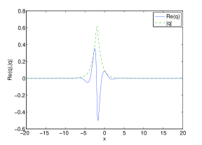
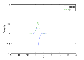
(a)(b)

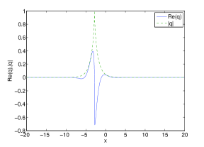
(c)

Figure 1: Envelope soliton for the complex short pulse equation (2), solid line: $Re(q)$, dashed line: $|q|$; (a) smooth soliton with $p_{1}=1+1.5\mathrm{i}$, (b) loop soliotn with $p_{1}=1+0.5\mathrm{i}$, (c) cuspon soliton with $p_{1}=1+\mathrm{i}$.

Remark 4.3.  The one-soliton solution to the short pulse equation (1) is of loop-type, which lacks physical meaning in the context of nonlinear optics. However, the one-soliton solution to the complex short pulse equation (2) is of breather-type, which allows physical meaning for optical pulse.

Remark 4.4.  When $|p_{1R}|<|p_{1I}|$, there is no singularity for one-soliton solution. Moreover, in view of $\eta_{1R}$ associated with the width of envelope soliton and $\eta_{1I}$ associated with the phase, it is obvious that this nonsingular envelope soliton can only contain a few optical cycle. This property coincides with the fact that the complex short pulse equation is derived for the purpose of describing ultra-short pulse propagation. When $|p_{1R}|=|p_{1I}|$, the soliton becomes cuspon-like one, which agrees with the results in [10] derived from a bidirectional model.

4.2.2 Two-soliton solution

Based on the $N$-soliton solution of the complex short pulse equation from (74)–(75), the tau-functions for two-soliton solution can be expanded for $N=2$

$$f=\mathrm{Pf}(a_{1},a_{2},a_{3},a_{4},b_{1},b_{2},b_{3},b_{4})$$

$$\quad=1+a_{1\bar{1}}e^{\eta_{1}+\bar{\eta}_{1}}+a_{1\bar{2}}e^{\eta_{1}+\bar{\eta}_{2}}+a_{2\bar{1}}e^{\eta_{2}+\bar{\eta}_{1}}+a_{2\bar{2}}e^{\eta_{2}+\bar{\eta_{2}}}$$

$$\qquad+|P_{12}|^{2}\left(a_{1\bar{1}}a_{2\bar{2}}P_{1\bar{2}}P_{2\bar{1}}-a_{1\bar{2}}a_{2\bar{1}}P_{1\bar{1}}P_{2\bar{2}}\right)e^{\eta_{1}+\eta_{2}+\bar{\eta}_{1}+\bar{\eta}_{2}}\,,$$ (85)

$$g=\mathrm{Pf}(d_{0},\beta_{1},a_{1},a_{2},a_{3},a_{4},b_{1},b_{2},b_{3},b_{4})$$

$$\quad=\alpha_{1}e^{\eta_{1}}+\alpha_{2}e^{\eta_{2}}+P_{12}\left(\alpha_{1}P_{1\bar{1}}a_{2\bar{1}}-\alpha_{2}P_{2\bar{1}}a_{1\bar{1}}\right)e^{\eta_{1}+\eta_{2}+\bar{\eta}_{1}}$$

$$\qquad+P_{12}\left(\alpha_{1}P_{1\bar{2}}a_{2\bar{2}}-\alpha_{2}P_{2\bar{2}}a_{1\bar{2}}\right)e^{\eta_{1}+\eta_{2}+\bar{\eta}_{2}}\,,$$ (86)

where

$$P_{ij}=\frac{p_{i}-p_{j}}{p_{i}+p_{j}}\,,\quad P_{i\bar{j}}=\frac{p_{i}-\bar{p}_{j}}{p_{i}+\bar{p}_{j}}\,,\quad a_{i\bar{j}}=\frac{\alpha_{i}\bar{\alpha}_{j}(p_{i}\bar{p}_{j})^{2}}{4(p_{i}+\bar{p}_{j})^{2}}\,,$$ (87)

and $\eta_{j}=p_{j}y+p_{j}^{-1}s$, $\bar{\eta}_{j}=\bar{p}_{j}y+\bar{p}_{j}^{-1}s$.

 

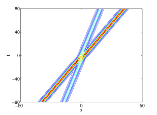
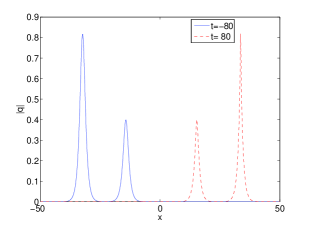
(a)(b)

Figure 2: Two-soliton solution to the complex short pulse equation (a) contour plot; (b) profiles at $t=-80$, $80$.

To avoid the singularity of the envelope solitons, the conditions $|p_{1R}|<|p_{1I}|$ and $|p_{2R}|<|p_{2I}|$ need to be satisfied. When two solitons stay apart, the amplitude of each soliton is of $2|p_{iR}|/|p_{i}|^{2}$, and the velocity is of $-1/|p_{i}|^{2}$ in the $ys$-coordinate system. Therefore, the soliton of larger velocity will catch up with and collide with the soliton of smaller velocity if it is initially located on the left. Furthermore, the collision is elastic, and there is no change in shape and amplitude of solitons except a phase shift. In Fig. 2, we illustrate the contour plot for the collision of two solitons (a), as well as the profiles (b) before and after the collision. The parameters are taken as $\alpha_{1}=\alpha_{2}=1.0$, $p_{1}=1+1.2\mathrm{i}$ and $p_{2}=1+2\mathrm{i}$.

Since the velocity of single envelope soliton is $-1/|p_{i}|^{2}$ in the $ys$-coordinate system, a bound state can be formed under the condition of $|p_{1}|^{2}=|p_{2}|^{2}$ if two solitons stay close enough and move with the same velocity. Such a bound state is shown in Fig. 3 for parameters chosen as $\alpha_{1}=\alpha_{2}=1.0$, $p_{1}=1.3+1.8193\mathrm{i}$, $p_{2}=1+2\mathrm{i}$. It is interesting that the envelope of the bound state oscillates periodically as it moves along $x$-axis.

 

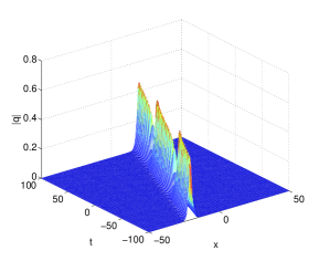
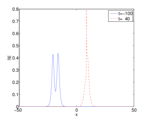
(a)(b)

Figure 3: Bound state to the complex short pulse equation: (a) 3D plot (b) profiles at $t=-100$, $40$.

4.3 Bilinear equations and $N$-soliton solutions to the coupled complex short pulse equation

Proposition 4.5.  The coupled complex short pulse equation is derived from bilinear equations

$$D_{s}D_{y}f\cdot g_{i}=fg_{i},\quad i=1,2\,,$$ (88)

$$D^{2}_{s}f\cdot f=\frac{1}{2}\left(|g_{1}|^{2}+|g_{2}|^{2}\right)\,,$$ (89)

by dependent variable transformation

$$q_{1}=\frac{g_{1}}{f},\quad q_{2}=\frac{g_{2}}{f}\,,$$ (90)

and hodograph transformation

$$x=y-2(\ln f)_{s}\,,\quad t=-s\,,$$ (91)

Proof. Dividing both sides of Eqs. (88)–(89) by $f^{2}$, we have

$$\left(\frac{g_{i}}{f}\right)_{sy}+2\frac{g_{i}}{f}\left(\ln f\right)_{sy}=\frac{g_{i}}{f}\,,$$ (92)

$$\left(\ln f\right)_{ss}=\frac{1}{4}\left(\frac{|g_{1}|^{2}}{f^{2}}+\frac{|g_{2}|^{2}}{f^{2}}\right)\,.$$ (93)

From dependent variable and hodograph transformations (90)–(91), we obtain

$$\frac{\partial x}{\partial s}=-2(\ln f)_{ss}=-\frac{1}{2}\left(|q_{1}|^{2}+|q_{2}|^{2}\right)\,,\qquad\frac{\partial x}{\partial y}=1-2(\ln f)_{sy}\,,$$

which implies

$${\partial_{y}}=\rho^{-1}{\partial_{x}}\,,\qquad{\partial_{s}}=-{\partial_{t}}-\frac{1}{2}\left(|q_{1}|^{2}+|q_{2}|^{2}\right){\partial_{x}}\,$$ (94)

by letting $1-2(\ln f)_{sy}=\rho^{-1}$.

With the use of (94), Eq. (92) can be recast into

$$\rho\left(\frac{g_{i}}{f}\right)_{sy}=\frac{g_{i}}{f}\,,\quad i=1,2\,,$$ (95)

which can be further converted into

$$\partial_{x}\left(-\partial_{t}-\frac{1}{2}(|q_{1}|^{2}+|q_{2}|^{2})\partial_{x}\right)q_{i}=q_{i}\,,\quad i=1,2\,.$$ (96)

Eq. (96) is, obviously, equivalent to the coupled complex short pulse equation (3)–(4).         

$N$-soliton solution for the coupled complex short pulse equation is given in a similar way as the complex short pulse equation by the following theorem.

Theorem 4.6.  The coupled complex short pulse equation admits the following $N$-soliton solution

$$q_{i}=\frac{g_{i}}{f},\quad x=y-2(\ln f)_{s}\,,\quad t=-s\,,$$

where $f$, $g_{i}$ are pfaffians defined as

$$f = \mathrm{Pf}(a_{1},\cdots,a_{2N},b_{1},\cdots,b_{2N})\,,$$ (97)

$$g_{i} = \mathrm{Pf}(d_{0},\beta_{i},a_{1},\cdots,a_{2N},b_{1},\cdots,b_{2N})\,,$$ (98)

and the elements of the pfaffians are determined as

$$\mathrm{Pf}(a_{j},a_{k})=\frac{p_{j}-p_{k}}{p_{j}+p_{k}}e^{\eta_{j}+\eta_{k}}\,,\quad\mathrm{Pf}(a_{j},b_{k})=\delta_{j,k}\,,$$ (99)

$$\mathrm{Pf}(b_{j},b_{k})=\frac{1}{4}\frac{\sum^{2}_{i=1}\alpha^{(i)}_{j}\alpha^{(i)}_{k}}{p^{-2}_{j}-p^{-2}_{k}}\delta_{\mu+1,\nu}\,,\quad\mathrm{Pf}(d_{l},a_{k})=p_{k}^{l}e^{\eta_{k}}\,,$$ (100)

$$\mathrm{Pf}(b_{j},\beta_{i})=\alpha^{(i)}_{j}\delta_{\mu,i}\,,\quad\mathrm{Pf}(d_{0},b_{j})=\mathrm{Pf}(d_{0},\beta_{i})=\mathrm{Pf}(a_{j},\beta_{i})=0\,.$$ (101)

Here $\mu=index(b_{j})$, $\nu=index(b_{k})$, $\eta_{j}=p_{j}y+p_{j}^{-1}s+\eta_{j,0}$ which satisfying $p_{j+N}=\bar{p}_{j}$, $\alpha_{j+N}=\bar{\alpha}_{j}$.

The proof of the Theorem is given in the Appendix. In the subsequent section, based on the $N$-soliton solution of coupled complex short pulse equation, we will investigate the dynamics of one- and two-solitons in details.

Remark 4.7.  Through the transformations

$$x=y-2(\ln f)_{s}\,,\quad t=-s\,,\quad q_{i}=\frac{g_{i}}{f}\,,$$ (102)

the vector complex short pulse equation (43) can be decomposed into the following bilinear equations

$$D_{s}D_{y}f\cdot g_{i}=fg_{i},\quad i=1,\cdots,n\,,$$ (103)

$$D^{2}_{s}f\cdot f=\frac{1}{2}\left(\sum^{n}_{i=1}|g_{i}|^{2}\right)\,.$$ (104)

The parametric form of $N$-soliton solution in terms of pfaffians to the vector complex short pulse equation (43) can be given in a very similar from as to to the coupled complex short pulse equation. Here, we omit the details and will report the results later on.

5 Dynamics of solitons to the coupled complex short pulse equation

5.1 One-soliton solution

The tau-functions for one-soliton solution to the coupled complex short pulse equation are obtained from (97)–(98) for $N=1$

$$f=-1-\frac{1}{4}\frac{\sum_{i=1}^{2}|\alpha^{(i)}_{1}|^{2}(p_{1}\bar{p}_{1})^{2}}{(p_{1}+\bar{p}_{1})^{2}}e^{\eta_{1}+\bar{\eta}_{1}}\,,$$ (105)

$$g_{1}=-\alpha^{(1)}_{1}e^{\eta_{1}}\,,\quad g_{2}=-\alpha^{(2)}_{1}e^{\eta_{1}}\,.$$ (106)

Let $p_{1}=p_{1R}+\mathrm{i}p_{1I}$, the one-soliton solution can be expressed in the following parametric form

$$\left(\begin{array}[]{c}q_{1}\\ q_{2}\end{array}\right)=\left(\begin{array}[]{c}A_{1}\\ A_{2}\end{array}\right)\frac{2p_{1R}}{|p_{1}|^{2}}e^{\mathrm{i}\eta_{1I}}{\mbox{sech}}\left(\eta_{1R}+\eta_{10}\right)\,,$$ (107)

$$x=y-\frac{2p_{1R}}{|p_{1}|^{2}}\left(\tanh(\eta_{1R}+\eta_{10})+1\right)\,,\quad t=-s\,,$$ (108)

where

$$\eta_{1R}=p_{1R}\left(y+\frac{1}{|p_{1}|^{2}}s\right),\quad\eta_{1I}=p_{1I}\left(y-\frac{1}{|p_{1}|^{2}}s\right)\,,$$ (109)

$$A_{i}=\frac{\alpha_{1}^{(i)}}{\sqrt{\sum_{i=1}^{2}|\alpha_{1}^{(i)}|^{2}}}\,,\quad\eta_{10}=\ln\frac{\sqrt{\sum_{i=1}^{2}|\alpha_{1}^{(i)}|^{2}}|p_{1}|^{2}}{4|p_{1R}|}\,.$$ (110)

The amplitudes of the single soliton in each component are ${2|A_{1}|p_{1R}}/{|p_{1}|^{2}}$ and ${2|A_{2}|p_{1R}}/{|p_{1}|^{2}}$, respectively. Note that $|A_{1}|^{2}+|A_{2}|^{2}=1$. Same as the analysis for one-soliton solution of complex short pulse equation, if $|p_{1R}|<|p_{1I}|$, the envelope for one-soliton in each of the component is smooth, whereas, if $|p_{1R}|>|p_{1I}|$, it becomes a loop (multi-valued) soliton, if $|p_{1R}|=|p_{1I}|$, it is a cuspon.

5.2 Soliton interactions

Two-soliton solution for coupled complex short pulse equation is obtained from (97)–(98) for $N=2$. By expanding the pfaffians, the tau-functions for two-soliton solution are expressed by

$$f=1+e^{\eta_{1}+\bar{\eta}_{1}+r_{1\bar{1}}}+e^{\eta_{1}+\bar{\eta}_{2}+r_{1\bar{2}}}+e^{\eta_{2}+\bar{\eta}_{1}+r_{2\bar{1}}}+e^{\eta_{2}+\bar{\eta}_{2}+r_{2\bar{2}}}$$

$$\qquad+|P_{12}|^{2}|P_{1\bar{2}}|^{2}P_{1\bar{1}}P_{2\bar{2}}\left(B_{1\bar{1}}B_{2\bar{2}}-B_{2\bar{1}}B_{1\bar{2}}\right)e^{\eta_{1}+\eta_{2}+\bar{\eta}_{1}+\bar{\eta}_{2}}\,,$$ (111)

$$g_{1}=\alpha^{(1)}_{1}e^{\eta_{1}}+\alpha^{(1)}_{2}e^{\eta_{2}}+P_{12}P_{1\bar{1}}P_{2\bar{1}}\left(\alpha^{(1)}_{2}B_{1\bar{1}}-\alpha^{(1)}_{1}B_{2\bar{1}}\right)e^{\eta_{1}+\eta_{2}+\bar{\eta}_{1}}$$

$$\qquad+P_{12}P_{1\bar{2}}P_{2\bar{2}}\left(\alpha^{(1)}_{2}B_{1\bar{2}}-\alpha^{(1)}_{1}B_{2\bar{2}}\right)e^{\eta_{1}+\eta_{2}+\bar{\eta}_{2}}\,,$$ (112)

$$g_{2}=\alpha_{1}^{(2)}e^{\eta_{1}}+\alpha_{2}^{(2)}e^{\eta_{2}}+P_{12}P_{1\bar{1}}P_{2\bar{1}}\left(\alpha_{2}^{(2)}B_{1\bar{1}}-\alpha_{1}^{(2)}B_{2\bar{1}}\right)e^{\eta_{1}+\eta_{2}+\bar{\eta}_{1}}$$

$$\qquad+P_{12}P_{1\bar{2}}P_{2\bar{2}}\left(\alpha_{2}^{(2)}B_{1\bar{2}}-\alpha_{1}^{(2)}B_{2\bar{2}}\right)e^{\eta_{1}+\eta_{2}+\bar{\eta}_{2}}\,,$$ (113)

where

$$P_{ij}=\frac{p_{i}-p_{j}}{p_{i}+p_{j}}\,,\quad P_{i\bar{j}}=\frac{p_{i}-\bar{p}_{j}}{p_{i}+\bar{p}_{j}}\,,$$

$$B_{i\bar{j}}=\frac{\alpha_{i}^{(1)}\bar{\alpha}_{j}^{(1)}+\alpha_{i}^{(2)}\bar{\alpha}_{j}^{(2)}}{4(p_{i}^{-2}-\bar{p}_{j}^{-2})}\,,\quad e^{r_{i\bar{j}}}=\frac{\alpha_{i}^{(1)}\bar{\alpha}_{j}^{(1)}+\alpha_{i}^{(2)}\bar{\alpha}_{j}^{(2)}}{4(p_{i}^{-1}+\bar{p}_{j}^{-1})^{2}}\,.$$

and $\eta_{j}=p_{j}y+p_{j}^{-1}s$, $p_{3}=\bar{p}_{1}$, $p_{4}=\bar{p}_{2}$, thus, $\eta_{3}=\bar{\eta}_{1}$, $\eta_{4}=\bar{\eta}_{2}$.

Next, we investigate the asymptotic behavior of two-soliton solution. To this end, we assume $p_{1R}>p_{2R}>0$, $p_{1R}/|p_{1}|^{2}>p_{2R}/|p_{2}|^{2}$ without loss of generality. For the above choice of parameters, we have (i) $\eta_{1R}\approx 0$, $\eta_{2R}\rightarrow\mp\infty$ as $t\rightarrow\mp\infty$ for soliton 1 and (ii) $\eta_{2R}\approx 0$, $\eta_{2R}\rightarrow\pm\infty$ as $t\rightarrow\mp\infty$ for soliton 2. This leads to the following asymptotic forms for two-soliton solution.
(i) Before collision ($t\rightarrow-\infty$)
Soliton 1 ($\eta_{1R}\approx 0$, $\eta_{2R}\rightarrow-\infty$):

$$\left(\begin{array}[]{c}q_{1}\\ q_{2}\end{array}\right) \rightarrow \left(\begin{array}[]{c}\alpha_{1}^{(1)}\\ \alpha_{1}^{(2)}\end{array}\right)\frac{e^{\eta_{1}}}{1+e^{\eta_{1}+\bar{\eta}_{1}+r_{1\bar{1}}}}\,,$$ (118)

$$\rightarrow \left(\begin{array}[]{c}A_{1}^{1-}\\ A_{2}^{1-}\end{array}\right)\frac{2p_{1R}}{|p_{1}|^{2}}e^{i\eta_{1I}}{\mbox{sech}}\left(\eta_{1R}+\frac{r_{1\bar{1}}}{2}\right)\,,$$ (121)

where

$$\left(\begin{array}[]{c}A_{1}^{1-}\\ A_{2}^{1-}\end{array}\right)=\left(\begin{array}[]{c}\alpha_{1}^{(1)}\\ \alpha_{1}^{(2)}\end{array}\right)\frac{1}{\sqrt{|\alpha_{1}^{(1)}|^{2}+|\alpha_{1}^{(2)}|^{2}}}\,.$$ (122)

Soliton 2 ($\eta_{2R}\approx 0$, $\eta_{1R}\to\infty$):

$$\left(\begin{array}[]{c}q_{1}\\ q_{2}\end{array}\right)\to\left(\begin{array}[]{c}A^{2-}_{1}\\ A^{2-}_{2}\end{array}\right)\frac{2p_{2R}}{|p_{2}|^{2}}e^{i\eta_{2I}}{\mbox{sech}}\left(\eta_{2R}+\frac{r_{1\bar{1}2\bar{2}}-r_{1\bar{1}}}{2}\right)\,,$$ (123)

where

$$\left(\begin{array}[]{c}A^{2-}_{1}\\ A^{2-}_{2}\end{array}\right)=\left(\begin{array}[]{c}e^{r^{(1)}_{1\bar{1}2}}\\ e^{r^{(2)}_{1\bar{1}2}}\end{array}\right)\frac{e^{-(r_{1\bar{1}2\bar{2}}+r_{1\bar{1}}-r_{2\bar{2}})/{2}}}{\sqrt{|\alpha^{(1)}_{2}|^{2}+|\alpha^{(2)}_{2}|^{2}}}\,,$$ (124)

with

$$e^{r^{(i)}_{1\bar{1}2}}=P_{12}P_{1\bar{1}}P_{2\bar{1}}\left(\alpha^{(i)}_{2}B_{1\bar{1}}-\alpha^{(i)}_{1}B_{2\bar{1}}\right)\,,\quad(i=1,2)$$ (125)

$$e^{r_{1\bar{1}2\bar{2}}}=|P_{12}|^{2}|P_{1\bar{2}}|^{2}P_{1\bar{1}}P_{2\bar{2}}\left(B_{1\bar{1}}B_{2\bar{2}}-B_{2\bar{1}}B_{1\bar{2}}\right)\,.$$ (126)

After collision ($t\to\infty$)
Soliton 1 ($\eta_{1R}\approx 0$, $\eta_{2R}\to\infty$):

$$\left(\begin{array}[]{c}q_{1}\\ q_{2}\end{array}\right)\rightarrow\left(\begin{array}[]{c}A_{1}^{1+}\\ A_{2}^{1+}\end{array}\right)\frac{2p_{1R}}{|p_{1}|^{2}}e^{i\eta_{1I}}{\mbox{sech}}\left(\eta_{2R}+\frac{r_{1\bar{1}2\bar{2}}-r_{2\bar{2}}}{2}\right)\,,$$ (127)

where

$$\left(\begin{array}[]{c}A_{1}^{1+}\\ A_{2}^{1+}\end{array}\right)=\left(\begin{array}[]{c}e^{r_{12\bar{1}}^{(1)}}\\ e^{r_{12\bar{1}}^{(2)}}\end{array}\right)\frac{e^{-(r_{1\bar{1}2\bar{2}}-r_{1\bar{1}}+r_{2\bar{2}})/{2}}}{\sqrt{|\alpha_{1}^{(1)}|^{2}+|\alpha_{1}^{(2)}|^{2}}}\,,$$ (128)

with

$$e^{r_{12\bar{1}}^{(i)}}=P_{12}P_{1\bar{2}}P_{2\bar{2}}\left(\alpha_{2}^{(i)}B_{1\bar{2}}-\alpha_{1}^{(i)}B_{2\bar{2}}\right)\,,\quad(i=1,2)\,.$$ (129)

Soliton 2 ($\eta_{2R}\approx 0$, $\eta_{1R}\rightarrow-\infty$):

$$\left(\begin{array}[]{c}q_{1}\\ q_{2}\end{array}\right)\rightarrow\left(\begin{array}[]{c}A_{1}^{2+}\\ A_{2}^{2+}\end{array}\right)\frac{2p_{2R}}{|p_{2}|^{2}}e^{i\eta_{2I}}{\mbox{sech}}\left(\eta_{2R}+\frac{r_{2\bar{2}}}{2}\right)\,,$$ (130)

where

$$\left(\begin{array}[]{c}A_{1}^{2+}\\ A_{2}^{2+}\end{array}\right)=\left(\begin{array}[]{c}\alpha_{2}^{(1)}\\ \alpha_{2}^{(2)}\end{array}\right)\frac{1}{\sqrt{|\alpha_{2}^{(1)}|^{2}+|\alpha_{2}^{(2)}|^{2}}}\,.$$ (131)

Similar to the analysis for the CNLS equations [38, 39, 40], the change in the amplitude of each of the solitons in each component can be obtained by introducing the transition matrix $T^{k}_{j}$ by $A_{j}^{k+}=T_{j}^{k}A_{j}^{k-}$, $j,k=1,2$. The elements of transition matrix is obtained from the above asymptotic analysis as

$$T_{j}^{1}=\left(\frac{P_{12}P_{1\bar{2}}}{\bar{P}_{12}\bar{P}_{1\bar{2}}}\right)^{1/2}\frac{1}{\sqrt{1-\lambda_{1}\lambda_{2}}}\left(1-\lambda_{2}\frac{\alpha_{2}^{(j)}}{\alpha_{1}^{(j)}}\right)\,,\quad j=1,2\,,$$ (132)

$$T_{j}^{2}=\left(\frac{\bar{P}_{12}P_{1\bar{2}}}{P_{12}\bar{P}_{1\bar{2}}}\right)^{1/2}\sqrt{1-\lambda_{1}\lambda_{2}}\left(1-\lambda_{1}\frac{\alpha_{1}^{(j)}}{\alpha_{2}^{(j)}}\right)^{-1}\,,\quad j=1,2\,,$$ (133)

where $\lambda_{1}=B_{2\bar{1}}/B_{1\bar{1}}$, $\lambda_{2}=B_{1\bar{2}}/B_{2\bar{2}}$.

Therefore, in general, there is an exchange of energies between two components of two solitons after the collision. An example is shown in Fig. 4 for the parameters taken as follows $p_{1}=1+1.2\mathrm{i}$, $p_{2}=1+2\mathrm{i}$, $\alpha^{(1)}_{1}=\alpha^{(2)}_{1}=1.0$, $\alpha^{(1)}_{2}=2.0$, $\alpha^{(2)}_{2}=1.0$.

 

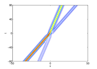
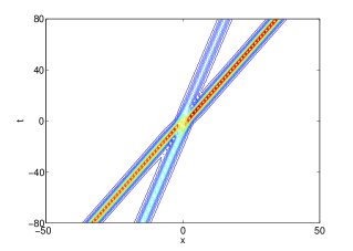
(a)(b)

 

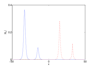
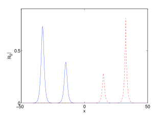
(c)(d)

Figure 4: Inelastic collision in coupled complex short pulse equation. (a)-(b): contour plot; (c)-(d): profiles before and after the collision.

However, only for the special case

$$\frac{\alpha_{1}^{(1)}}{\alpha_{2}^{(1)}}=\frac{\alpha_{1}^{(2)}}{\alpha_{2}^{(2)}}\,,$$ (134)

there is no energy exchange between two compoents of solitons after the collision. An example is shown in Fig. 5 for the parameters $p_{1}=1+1.2\mathrm{i}$, $p_{2}=1+2\mathrm{i}$, $\alpha^{(1)}_{1}=\alpha^{(2)}_{1}=1.0$,  $\alpha^{(1)}_{2}=\alpha^{(2)}_{2}=1.0$.

 

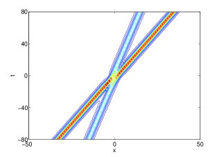
(a)(b)

 

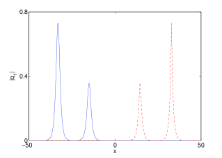
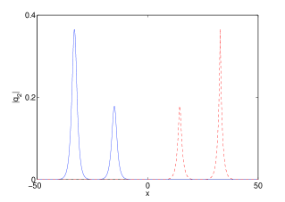
(c)(d)

Figure 5: Elastic collision in coupled complex short pulse equation.

It is interesting to note that if we just change the parameters in previous two examples as $\alpha^{(1)}_{2}=0$, $\alpha^{(2)}_{2}=1.0$, the energy of one soliton is concentrated in component $q_{2}$ before the collision. However, component $q_{1}$ gains some energy after the collision. Such an example is shown in Fig. 6.

 

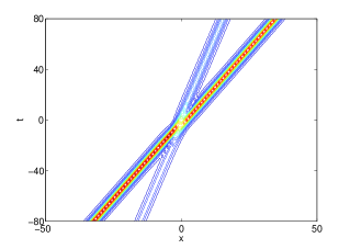
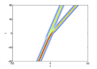
(a)(b)

 

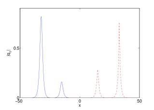
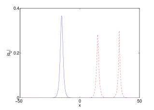
(c)(d)

Figure 6: Inelastic collision in coupled complex short pulse equation for $p_{1}=1+1.2{\rm i}$, $p_{2}=1+2{\rm i}$, $\alpha^{(1)}_{1}=\alpha^{(2)}_{1}=1.0$, $\alpha^{(1)}_{2}=0$, $\alpha^{(2)}_{2}=1.0$. (a)-(b): contour plot; (c)-(d): profiles before and after the collision.

On the other hand, if we change the parameters as $\alpha^{(1)}_{2}=1.0$, $\alpha^{(2)}_{2}=0$, then the energy of one soliton, which are distributed between two components before the collision is concentrated into one component $q_{2}$ after the collision. The example is shown in Fig. 7.

 

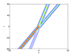
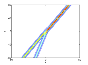
(a)(b)

 

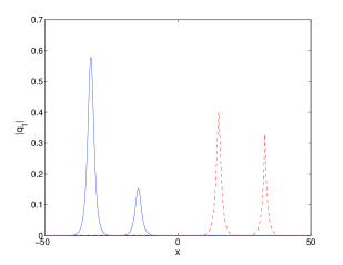
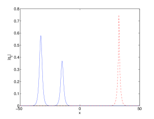
(c)(d)

Figure 7: Inelastic collision in coupled complex short pulse equation for $p_{1}=1+1.2\mathrm{i}$, $p_{2}=1+2\mathrm{i}$, $\alpha^{(1)}_{1}=\alpha^{(2)}_{1}=1.0$,  $\alpha^{(1)}_{2}=1.0$, $\alpha^{(2)}_{2}=0$. (a)-(b): contour plot; (c)-(d): profiles before and after the collision.

6 Concluding Remarks

In this paper, we proposed a complex short pulse equation and its two-component generalization. Both of the equations can be used to model the propagation of ultra-short pulses in optical fibers. We have shown their integrability by finding the Lax pairs and infinite numbers of conservation laws. Furthermore, multi-soliton solutions are constructed via Hirota’s bilinear method. In particular, one-soliton solution for the CSP equation is an envelope soliton with a few optical cycles under certain condition, which perfectly match the requirement for the ultra-short pulses. The $N$-solution for complex short pulse equation and its two-component generalization is a benchmark for the study of soliton interactions in ultra-short pulses propagation in optical fibers. It is expected that these analytical solutions can be confirmed from experiments.

Similar to our previous results for the integrable discretizations of the short pulse equation [22], how to construct integrable discretizations of the CSP and coupled CSP equations and how to apply them for the numerical simulations is also an interesting topic to be studied. It is obviously beyond the scope of the present paper, we are to report the results on this aspect in a forthcoming paper.

Appendix

Proof of Theorem 4.2

Proof. First we define

$$(b_{j},\bar{\beta}_{1})=\bar{\alpha}_{j}\delta_{\mu,1}\,,\quad(b_{j},\bar{\beta}_{2})=\bar{\alpha}_{j}\delta_{\mu,2}\,,$$

where $index(b_{j})=\mu$ , then from the fact

$$\mathrm{Pf}(\bar{a}_{j},a_{k})=\mathrm{Pf}(a_{N+j},a_{N+k})\,,\mathrm{Pf}(\bar{b}_{j},b_{k})=\mathrm{Pf}(b_{N+j},b_{N+k})\,,$$

we obtain

$$\bar{f}=f\,,\quad\bar{g}=\mathrm{Pf}(d_{0},\bar{\beta}_{1},a_{1},\cdots,a_{2N},b_{1},\cdots,b_{2N})\,.$$

Since

$$\frac{\partial}{\partial y}\mathrm{Pf}(a_{j},a_{k})=(p_{j}-p_{k})e^{\eta_{j}+\eta_{k}}=\mathrm{Pf}(d_{0},d_{1},a_{j},a_{k})\,,$$

$$\frac{\partial}{\partial s}\mathrm{Pf}(a_{j},a_{k})=(p^{-1}_{k}-p^{-1}_{j})e^{\eta_{j}+\eta_{k}}=\mathrm{Pf}(d_{-1},d_{0},a_{j},a_{k})\,,$$

$$\frac{\partial^{2}}{\partial s^{2}}\mathrm{Pf}(a_{j},a_{k})=(p^{-2}_{k}-p^{-2}_{j})e^{\eta_{j}+\eta_{k}}=\mathrm{Pf}(d_{-2},d_{0},a_{j},a_{k})\,,$$

$$\frac{\partial^{2}}{\partial y\partial s}\mathrm{Pf}(a_{j},a_{k})=(p_{j}p^{-1}_{k}-p_{k}p^{-1}_{j})e^{\eta_{j}+\eta_{k}}=\mathrm{Pf}(d_{-1},d_{1},a_{i},a_{j})\,,$$

we then have

$$\frac{\partial f}{\partial y}=\mathrm{Pf}(d_{0},d_{1},\cdots)\,,$$

$$\frac{\partial f}{\partial s}=\mathrm{Pf}(d_{-1},d_{0},\cdots)\,,$$

$$\frac{\partial^{2}f}{\partial s^{2}}=\mathrm{Pf}(d_{-2},d_{0},\cdots)\,,$$

$$\frac{\partial^{2}f}{\partial y\partial s}=\mathrm{Pf}(d_{-1},d_{1},\cdots)\,.$$

Here $\mathrm{Pf}(d_{0},d_{1},a_{1},\cdots,a_{2N},b_{1},\cdots,b_{2N})$ is abbreviated by $\mathrm{Pf}(d_{0},d_{1},\cdots)$, so as other similar pfaffians.

Furthermore, it can be shown

$$\frac{\partial g}{\partial y}=\frac{\partial}{\partial y}\left[\sum_{j=1}^{2N}(-1)^{j}\mathrm{Pf}(d_{0},a_{j})\mathrm{Pf}(\beta_{1},\cdots,\hat{a}_{j},\cdots)\right]$$

$$=\sum_{j=1}^{2N}(-1)^{j}\left[\left({\partial_{y}}\mathrm{Pf}(d_{0},a_{j})\right)\mathrm{Pf}(\beta_{1},\cdots,\hat{a}_{j},\cdots)+\mathrm{Pf}(d_{0},a_{j}){\partial_{y}}\mathrm{Pf}(\beta_{1},\cdots,\hat{a}_{j},\cdots)\right]$$

$$=\sum_{j=1}^{2N}(-1)^{j}\left[\mathrm{Pf}(d_{1},a_{j})\mathrm{Pf}(\beta_{1},\cdots,\hat{a}_{j},\cdots)+\mathrm{Pf}(d_{0},a_{j})\mathrm{Pf}(\beta_{1},d_{0},d_{1},\cdots,\hat{a}_{j},\cdots)\right]$$

$$=\mathrm{Pf}(d_{1},\beta_{1},\cdots)+\mathrm{Pf}(d_{0},\beta_{1},d_{0},d_{1},\cdots)$$

$$=\mathrm{Pf}(d_{1},\beta_{1},\cdots)\,.$$

Here $\hat{a}_{j}$ means that the index $j$ is omitted. Similarly, we can show

$$\frac{\partial g}{\partial s}=\mathrm{Pf}(d_{-1},\beta_{1},\cdots)\,,$$

$$\frac{\partial^{2}g}{\partial y\partial s}=\frac{\partial}{\partial y}\left[\sum_{j=1}^{2N}(-1)^{j}\mathrm{Pf}(d_{-1},a_{j})\mathrm{Pf}(\beta_{1},\cdots,\hat{a}_{j},\cdots)\right]$$

$$=\sum_{j=1}^{2N}(-1)^{j}\left[\left({\partial_{y}}\mathrm{Pf}(d_{-1},a_{j})\right)\mathrm{Pf}(\beta_{1},\cdots,\hat{a}_{j},\cdots)+\mathrm{Pf}(d_{-1},a_{j}){\partial_{y}}\mathrm{Pf}(\beta_{1},\cdots,\hat{a}_{j},\cdots)\right]$$

$$=\sum_{j=1}^{2N}(-1)^{j}\left[\mathrm{Pf}(d_{0},a_{j})\mathrm{Pf}(\beta_{1},\cdots,\hat{a}_{j},\cdots)+\mathrm{Pf}(d_{-1},a_{j})\mathrm{Pf}(\beta_{1},d_{0},d_{1},\cdots,\hat{a}_{j},\cdots)\right]$$

$$=\mathrm{Pf}(d_{0},\beta_{1},\cdots)+\mathrm{Pf}(d_{-1},\beta_{1},d_{0},d_{1},\cdots)\,.$$

An algebraic identity of pfaffian [21]

$$\mathrm{Pf}(d_{-1},\beta_{1},d_{0},d_{1},\cdots)\mathrm{Pf}(\cdots)=\mathrm{Pf}(d_{-1},d_{0},\cdots)\mathrm{Pf}(d_{1},\beta_{1},\cdots)$$

$$\quad-\mathrm{Pf}(d_{-1},d_{1},\cdots)\mathrm{Pf}(d_{0},\beta_{1},\cdots)+\mathrm{Pf}(d_{-1},\beta_{1},\cdots)\mathrm{Pf}(d_{0},d_{1},\cdots)\,,$$

implies

$$({\partial_{s}}{\partial_{y}}g-g)\times f={\partial_{s}}f\times{\partial_{y}}g-{\partial_{s}}{\partial_{y}}f\times g+{\partial_{s}}g\times{\partial_{y}}f\,.$$

Therefore, the first bilinear equation is approved.

The second bilinear equation can be proved in the same way by Iwao and Hirota [37].

$$\frac{\partial^{2}f}{\partial s^{2}}\times 0-\frac{\partial f}{\partial s}\frac{\partial f}{\partial s}$$

$$=\mathrm{Pf}(d_{-2},d_{0},\cdots)\mathrm{Pf}(d_{0},d_{0},\cdots)-\mathrm{Pf}(d_{-1},d_{0},\cdots)\mathrm{Pf}(d_{-1},d_{0},\cdots)$$

$$=\sum_{i=1}^{2N}(-1)^{i}\mathrm{Pf}(d_{-2},a_{i})\mathrm{Pf}(d_{0},\cdots,\hat{a}_{i},\cdots)\sum_{j=1}^{2N}(-1)^{j}\mathrm{Pf}(d_{0},a_{j})\mathrm{Pf}(d_{0},\cdots,\hat{a}_{j},\cdots)$$

$$-\sum_{i=1}^{2N}(-1)^{i}\mathrm{Pf}(d_{-1},a_{i})\mathrm{Pf}(d_{0},\cdots,\hat{a}_{i},\cdots)\sum_{j=1}^{2N}(-1)^{j}\mathrm{Pf}(d_{-1},a_{j})\mathrm{Pf}(d_{0},\cdots,\hat{a}_{j},\cdots)$$

$$=\sum_{i,j=1}^{2N}(-1)^{i+j}\left[\mathrm{Pf}(d_{-2},a_{i})\mathrm{Pf}(d_{0},a_{j})-\mathrm{Pf}(d_{-1},a_{i})\mathrm{Pf}(d_{-1},a_{j})\right]$$

$$\quad\times\mathrm{Pf}(d_{0},\cdots,\hat{a}_{i},\cdots)\mathrm{Pf}(d_{0},\cdots,\hat{a}_{j},\cdots)$$

$$=\sum_{i,j=1}^{2N}(-1)^{i+j+1}\left[p_{i}^{-2}+p_{i}^{-1}p_{j}^{-1}\right]\mathrm{Pf}(a_{i},a_{j})\mathrm{Pf}(d_{0},\cdots,\hat{a}_{i},\cdots)\mathrm{Pf}(d_{0},\cdots,\hat{a}_{j},\cdots)$$

The summation over the second term within the bracket vanishes due to the fact that

$$\sum_{i,j=1}^{2N}(-1)^{i+j+1}p_{i}^{-1}p_{j}^{-1}\mathrm{Pf}(a_{i},a_{j})\mathrm{Pf}(d_{0},\cdots,\hat{a}_{i},\cdots)\mathrm{Pf}(d_{0},\cdots,\hat{a}_{j},\cdots)$$

$$=\sum_{j,i=1}^{2N}(-1)^{j+i+1}p_{j}^{-1}p_{i}^{-1}\mathrm{Pf}(a_{j},a_{i})\mathrm{Pf}(d_{0},\cdots,\hat{a}_{j},\cdots)\mathrm{Pf}(d_{0},\cdots,\hat{a}_{i},\cdots)$$

$$=-\sum_{i,j=1}^{2N}(-1)^{i+j+1}p_{i}^{-1}p_{j}^{-1}\mathrm{Pf}(a_{i},a_{j})\mathrm{Pf}(d_{0},\cdots,\hat{a}_{i},\cdots)\mathrm{Pf}(d_{0},\cdots,\hat{a}_{j},\cdots)\,.$$

Therefore,

$$-\frac{\partial f}{\partial s}\frac{\partial f}{\partial s}=\sum_{i,j=1}^{2N}(-1)^{i+j+1}p_{i}^{-2}\mathrm{Pf}(a_{i},a_{j})\mathrm{Pf}(d_{0},\cdots,\hat{a}_{i},\cdots)\mathrm{Pf}(d_{0},\cdots,\hat{a}_{j},\cdots)$$

$$=\sum_{i=1}^{2N}(-1)^{i+1}p_{i}^{-2}\mathrm{Pf}(d_{0},\cdots,\hat{a}_{i},\cdots)\left[\sum_{j=1}^{2N}(-1)^{j}\mathrm{Pf}(a_{i},a_{j})\mathrm{Pf}(d_{0},\cdots,\hat{a}_{j},\cdots)\right]$$

Further, we note that the following identity can be substituted into the term within bracket

$$\sum_{j=1}^{2N}(-1)^{j}\mathrm{Pf}(a_{i},a_{j})\mathrm{Pf}(d_{0},\cdots,\hat{a}_{j},\cdots)$$

$$=\mathrm{Pf}(d_{0},a_{i})\mathrm{Pf}(\cdots)+(-1)^{i+1}\mathrm{Pf}(d_{0},\cdots,\hat{b}_{i},\cdots)\,$$

which is obtained from the expansion of the following vanishing pfaffian $\mathrm{Pf}(a_{i},d_{0},\cdots)$ on $a_{i}$. Consequently, we have

$$-\frac{\partial f}{\partial s}\frac{\partial f}{\partial s}=$$

$$\sum_{i=1}^{2N}(-1)^{i+1}p_{i}^{-2}\mathrm{Pf}(d_{0},\cdots,\hat{a}_{i},\cdots)\left[\mathrm{Pf}(d_{0},a_{i})\mathrm{Pf}(\cdots)+(-1)^{i+1}\mathrm{Pf}(d_{0},\cdots,\hat{b}_{i},\cdots)\right]\,,$$

$$=-\mathrm{Pf}(\cdots)\mathrm{Pf}(d_{-2},d_{0},\cdots)+\sum_{i=1}^{2N}p_{i}^{-2}\mathrm{Pf}(d_{0},\cdots,\hat{a}_{i},\cdots)\mathrm{Pf}(d_{0},\cdots,\hat{b}_{i},\cdots)\,,$$ (A.1)

which can be rewritten as

$$\frac{\partial^{2}f}{\partial s^{2}}f-\frac{\partial f}{\partial s}\frac{\partial f}{\partial s}=\sum_{i=1}^{2N}p_{i}^{-2}\mathrm{Pf}(d_{0},\cdots,\hat{a}_{i},\cdots)\mathrm{Pf}(d_{0},\cdots,\hat{b}_{i},\cdots)\,.$$ (A.2)

Now, we work on the r.h.s of the second bilinear equation.

$$\frac{1}{2}|g|^{2}=\frac{1}{2}\mathrm{Pf}(d_{0},\beta_{1},\cdots)\mathrm{Pf}(d_{0},\bar{\beta}_{1},\cdots)$$

$$=\frac{1}{2}\sum_{i,j}^{2N}(-1)^{i+j}\mathrm{Pf}(b_{i},\beta_{1})\mathrm{Pf}(d_{0},\cdots,\hat{b}_{i},\cdots)\mathrm{Pf}(b_{j},\bar{\beta}_{1})\mathrm{Pf}(d_{0},\cdots,\hat{b}_{j},\cdots)$$

$$=\frac{1}{4}\sum_{i,j}^{2N}(-1)^{i+j}(\alpha_{i}\bar{\alpha}_{j})\mathrm{Pf}(d_{0},\cdots,\hat{b}_{i},\cdots)\mathrm{Pf}(d_{0},\cdots,\hat{b}_{j},\cdots)$$

$$=\sum_{i,j}^{2N}(-1)^{i+j}\left(p_{i}^{-2}-p_{j}^{-2}\right)\mathrm{Pf}(b_{i},b_{j})\mathrm{Pf}(d_{0},\cdots,\hat{b}_{i},\cdots)\mathrm{Pf}(d_{0},\cdots,\hat{b}_{j},\cdots)$$

Next, the expansion of the vanishing pfaffian $\mathrm{Pf}(b_{i},d_{0},\cdots)$ on $b_{i}$ yields

$$\sum_{j=1}^{2N}(-1)^{i+j}\mathrm{Pf}(b_{i},b_{j})\mathrm{Pf}(d_{0},\cdots,\hat{b}_{j},\cdots)=\mathrm{Pf}(d_{0},\cdots,\hat{a}_{i},\cdots)\,,$$ (A.4)

which subsequently leads to

$$\sum_{i,j}^{2N}(-1)^{i+j}p_{i}^{-2}\mathrm{Pf}(b_{i},b_{j})\mathrm{Pf}(d_{0},\cdots,\hat{b}_{i},\cdots)\mathrm{Pf}(d_{0},\cdots,\hat{b}_{j},\cdots)$$

$$=\sum_{i}^{2N}p_{i}^{-2}\mathrm{Pf}(d_{0},\cdots,\hat{a}_{i},\cdots)\mathrm{Pf}(d_{0},\cdots,\hat{b}_{i},\cdots)\,.$$ (A.5)

Similarly, we can show that

$$-\sum_{i,j}^{2N}(-1)^{i+j}p_{j}^{-2}\mathrm{Pf}(b_{i},b_{j})\mathrm{Pf}(d_{0},\cdots,\hat{b}_{i},\cdots)\mathrm{Pf}(d_{0},\cdots,\hat{b}_{j},\cdots)$$

$$=\sum_{j}^{2N}p_{j}^{-2}\mathrm{Pf}(d_{0},\cdots,\hat{a}_{j},\cdots)\mathrm{Pf}(d_{0},\cdots,\hat{b}_{j},\cdots)\,.$$ (A.6)

Substituting Eqs. (A.5)–(A.5) into Eq. (Appendix), we arrive at

$$\frac{1}{2}|g|^{2}=2\sum_{i}^{2N}p_{i}^{-2}\mathrm{Pf}(d_{0},\cdots,\hat{a}_{i},\cdots)\mathrm{Pf}(d_{0},\cdots,\hat{b}_{i},\cdots)\,.$$ (A.7)

Consequently we have

$$2\frac{\partial^{2}f}{\partial s^{2}}f-2\frac{\partial f}{\partial s}\frac{\partial f}{\partial s}=\frac{1}{2}|g|^{2}\,,$$ (A.8)

which is nothing but the second bilinear equation. Therefore, the proof is complete.         

The proof of Theorem 4.6

Proof. The proof of the first bilinear equation can be done exactly in the same way as for the complex short pulse equation. In what follows, we prove the second equation by starting from the r.h.s of this equation. Because

$$\bar{g}_{1}=\mathrm{Pf}(d_{0},\bar{\beta}_{1},a_{1},\cdots,a_{2N},b_{1},\cdots,b_{2N})\,,$$

$$\bar{g}_{2}=\mathrm{Pf}(d_{0},\bar{\beta}_{2},a_{1},\cdots,a_{2N},b_{1},\cdots,b_{2N})\,,$$

the r.h.s of the bilinear equation turns out to be

$$\frac{1}{2}\left(g_{1}\bar{g}_{1}+g_{2}\bar{g}_{2}\right)$$

$$=\frac{1}{2}\sum^{2}_{k=1}\sum_{i,j}^{2N}(-1)^{i+j}\mathrm{Pf}(b_{i},\beta_{k})\mathrm{Pf}(d_{0},\cdots,\hat{b}_{i},\cdots)\mathrm{Pf}(b_{j},\bar{\beta}_{k})\mathrm{Pf}(d_{0},\cdots,\hat{b}_{j},\cdots)$$

$$=\frac{1}{4}\sum_{i,j}^{2N}(-1)^{i+j}\sum^{2}_{k=1}(\alpha^{(k)}_{i}\bar{\alpha}^{(k)}_{j})\mathrm{Pf}(d_{0},\cdots,\hat{b}_{i},\cdots)\mathrm{Pf}(d_{0},\cdots,\hat{b}_{j},\cdots)$$

$$=\sum_{i,j}^{2N}(-1)^{i+j}\left(p_{i}^{-2}-p_{j}^{-2}\right)\mathrm{Pf}(b_{i},b_{j})\mathrm{Pf}(d_{0},\cdots,\hat{b}_{i},\cdots)\mathrm{Pf}(d_{0},\cdots,\hat{b}_{j},\cdots)$$

Similar to the complex short pulse equation, we can show

$$\frac{1}{2}\left(|g_{1}|^{2}+|g_{2}|^{2}\right)=2\sum_{i}^{2N}p_{i}^{-2}\mathrm{Pf}(d_{0},\cdots,\hat{a}_{i},\cdots)\mathrm{Pf}(d_{0},\cdots,\hat{b}_{i},\cdots)\,.$$ (A.10)

Regarding the r.h.s of the bilinear equation, exactly the same as the proof of the Theorem 4.2, we have

$$\frac{\partial^{2}f}{\partial s^{2}}f-\frac{\partial f}{\partial s}\frac{\partial f}{\partial s}=\sum_{i}^{2N}p_{i}^{-2}\mathrm{Pf}(d_{0},\cdots,\hat{a}_{i},\cdots)\mathrm{Pf}(d_{0},\cdots,\hat{b}_{i},\cdots)\,.$$ (A.11)

Therefore the second bilinear equation is proved.

References

- [1] A. Hasegawa, Y. Kodama, Solitons in Optical Communications (Oxford University Press, 1995).
- [2] G. P. Agrawal, Nonlinear Fiber Optics (Academic, San Diego, 2001).
- [3] R. W. Boyd, Nonlinear Optics (Academic Press, Boston, 1992).
- [4] A. Yariv, P. Yeh, Optical Waves in Crystals: Propagation and Control of Laser Radiation (Wiley-Interscience, 1983).
- [5] V. E. Zakharov, A. B. Shabat, Eaxct theory of two-dimensional self-focusing and one-dimensional self-modulation of waves in nonlinear media, JETP 34 (1972) 62–69.
- [6] J. E. Rothenberg, Space-time focusing: breakdown of the slowly varying envelope approximation in the self-focusing of femtosecond pulses, Opt. Lett. 17 (1992) 1340-1342.
- [7] T. Schäfer, C. E. Wayne, Propagation of ultra-short optical pulses in cubic nonlinear media, Physica D 196 (2004) 90–105.
- [8] S.A. Skobelev, D.V. Kartasholv, A.V. Kim, Solitary-wave solutions for few-cycle optical pulses, Phys. Rev. Lett. 99 (2007) 203902.
- [9] A.V. Kim, S.A. Skobelev, D. Anderson, T. Hansson, M. Lisak, Extreme nonlinear optics in a Kerr medium: Exact soliton solutions for a few cycles, Phys. Rev. A 77 (2008) 043823.
- [10] S. Amiranashvili, A. G. Vladimirov, U. Bandelow Few-optical-cycle solitons and pulse self-compression in a Kerr medium, Phys. Rev. A 77 (2008) 063821.
- [11] M.L. Robelo, On equations which describe pseudospherical surfaces, Stud. Appl. Math. 81(1989) 221–248.
- [12] R. Beals, M. Rabelo, K. Tenenblat, Bäcklund transformations and inverse scattering solutions for some pseudospherical surface equations, Stud. Appl. Math. 81 (1989) 125–151.
- [13] A. Sakovich, S. Sakovich, The short pulse equation is integrable, J. Phys. Soc. Jpn. 74 (2005) 239–241.
- [14] J. C. Brunelli, The short pulse hierarchy, J. Math. Phys., 46(2005) 123507
- [15] J. C. Brunelli, The bi-Hamiltonian structure of the short pulse equation, Phys. Lett. A, 353(2006) 475–478.
- [16] A. Sakovich, S. Sakovich, Solitary wave solutions of the short pulse equation, J. Phys. A, 39(2006) L361–L367.
- [17] V. K. Kuetche, T. B. Bouetou, T. C. Kofane, On two-loop soliton solution of the Schäfer-Wayne short-pulse equation using Hirota’s method and Hodnett-Moloney approach, J. Phys. Soc. Jpn. 76 (2007) 024004.
- [18] E. Parkes, Some periodic and solitary tralvelling-wave solutions of the short pulse equation, Chaos Solitons Fractals, 38 (2008) 154-159.
- [19] Y. Matsuno, Multisoliton and multibreather solutions of the short pulse model equation, J. Phys. Soc. Jpn., 76 (2007) 084003.
- [20] Y. Matsuno, Periodic solutions of the short pulse model equation, J. Math. Phys., 49 (2008) 073508.
- [21] R. Hirota, 2004 The Direct Method in Soliton Theory, Cambridge University Press.
- [22] B.-F. Feng, K. Maruno, Y. Ohta, Integrable discretization of the short pulse equation, J. Phys. A 43 (2010) 085203.
- [23] B.-F. Feng , J. Inoguchi, K. Kajiwara, K. Maruno, Y. Ohta, Discrete integrable systems and hodograph transformations arising from motions of discrete plane curves, J. Phys. A 44 (2011) 395201.
- [24] L. Kurt, Y. Chung, T. Schäfer, Higher-order corrections to the short pulse equation, 46 (2013) 285202. J. Phys. A, 39(2006) L361–L367.
- [25] S. V. Manakov, On the theory of two-dimensional stationary self-focusing of electromagnetic waves, 38(1974) 248-253.
- [26] M. Pietrzyk, I. Kanattšikov, U. Bandelow On the propagation of vector ultra-short pulses, J. Nonlinear Math. Phys. 15 (2008) 162-170.
- [27] S. Sakovich, On integrability of the vector short pulse equation, J. Phys. Soc. Jpn. 77 (2008) 123001.
- [28] A. Dimakis, F. Muller-Hoissen, Bidifferential calculus approach to AKNS hierarchies and their solutions, SIGMA 6 (2010) 055.
- [29] Y. Matsuno, A novel multi-component generalization of the short pulse equation and its multisoliton solutions, J. Math. Phys., 52 (2011) 123702.
- [30] B.-F. Feng, An integrable coupled short pulse equation, J. Phys. A 45 (2012) 085202.
- [31] Y. Yao, Y. Zeng, Coupled short pulse hierarchy and its Hamiltonian structure, J. Phys. Soc. Jpn. 80 (2011) 064004.
- [32] J. C. Brunelli, S. Sakovich, Hamiltonian integrability of two-component short pulse equations, J. Math. Phys., 54 (2013) 012701.
- [33] T. Tsuchida, M. Wadati, The coupled modified Korteweg-de Vries equations, J. Phys. Soc. Jpn. 67 (1998) 1175-1187.
- [34] M. Wadati, H. Sanuki, K. Konno, Relations among inverse method, Bäcklund transformation and an infinite number of conservation Laws, Prog. Theor. Phys. 53(1975) 419-435.
- [35] M. Wadati, K. Konno, Y. H. Ichikawa, New Integrable Nonlinear Evolution Equations, J. Phys. Soc. Jpn. 47 (1979) 1698-1700.
- [36] G.S. Franca, J.F. Gomes, A.H. Zimerman, The higher grading structure of the WKI hierarchy and the two-component short pulse equation, J. High Energy Phys. 8(2012) 120.
- [37] M. Iwao, R. Hirota, Soliton solutions of a coupled modified KdV equations, J. Phys. Soc. Jpn. 66 (1997) 577–588.
- [38] R. Radhakrishnan, M. Lakshmanan, and J. Hietarinta, Inelastic collision and switching of coupled bright solitons in optical fibers, Phys. Rev. E 56 (1997) 2213–2216.
- [39] T. Kanna and M. Lakshmanan, Exact Soliton Solutions, Shape Changing Collisions, and Partially Coherent Solitons in Coupled Nonlinear Schrödinger Equations, Phys. Rev. Lett. 86 (2001) 5043-5046.
- [40] T. Kanna and M. Lakshmanan, Exact soliton solutions of coupled nonlinear Schrödinger equations: Shape-changing collisions, logic gates, and partially coherent solitons, Phys. Rev. E 67 (2003) 046617.